Beyond Gaussian pair fluctuation theory for strongly interacting Fermi gases

Abstract

Interacting Fermi systems in the strongly correlated regime play a fundamental role in many areas of physics and are of particular interest to the condensed matter community. Though weakly interacting fermions are understood, strongly correlated fermions are difficult to describe theoretically as there is no small interaction parameter to expand about. Existing strong coupling theories rely heavily on the so-called many-body $T$-matrix approximation that sums ladder-type Feynman diagrams. Here, by acknowledging the fact that the effective interparticle interaction (i.e., the vertex function) becomes smaller above three dimensions, we propose an alternative way to reorganize Feynman diagrams and develop a theoretical framework for interacting Fermi gases beyond the ladder approximation. As an application, we solve the equation of state for three- and two-dimensional strongly interacting fermions and find excellent agreement with experimental [Science 335, 563 (2012)] and other theoretical results above the temperature $0.5T_{F}$.

Using Feshbach resonances to tune the $s$-wave scattering length of two-component atomic Fermi gases Bloch2008 ; Giorgini2008 ; Chin2010 , the experimental exploration of the crossover from Bose-Einstein condensates (BEC) to Bardeen-Cooper-Schrieffer (BCS) superfluids in both three (3D) Ketterle2008 ; Nascimbene2010 ; Horikoshi2010 ; Ku2012 and two dimensions (2D) Martiyanov2010 ; Frohlich2011 ; Feld2011 ; Dyke2011 ; Makhalov2014 ; Murthy2015 ; Dyke2016 ; Fenech2016 ; Boettcher2016 has attracted significant attention for understanding strongly interacting phenomena. This has offered insight to other strongly interacting systems such as high-$T_{c}$ superconductors Lee2006RMP , nuclear matter Lee2006PRA and quark-gluon plasma Kolb2004 . These experiments have given a unique challenge to theorists as strongly correlated matter cannot be quantitatively described by a simple mean-field theory.

For strongly interacting systems, exact treatments only exist in some limiting situations, for example, Bethe ansatz solutions in one dimension Guan2013 , virial expansion at high temperature Liu2009 ; Leyronas2011 ; Rakshit2012 ; Liu2013 and Tan relations at large momentum Tan2008a ; Tan2008b ; Tan2008c ; Braaten2008 . Numerically exact and sophisticated quantum Monte Carlo (QMC) simulations have also been developed Astrakharchik2004 ; Bulgac2006 ; Houcke2012 ; Shi2015 ; Anderson2015 , however, these approaches have their own difficulty evaluating experimentally relevant observables. In addition to the exact techniques, there have been many attempts to solve strongly interacting fermions through approximate diagrammatic theories. A commonly used approximation is to sum over the complete geometric series of ladder diagrams, leading to the Gaussian pair fluctuation (GPF) theory Nozieres1985 ; SadeMelo1993 ; Hu2006 ; Liu2006 ; Parish2007 ; Diener2008 ; Watanabe2013 ; Marsiglio2015 ; He2015 ; Bighin2016 . Though the GPF theory seems to provide consistent predictions for recent experiments within certain errors Hu2008 ; Hu2010 ; Mulkerin2015 , it is hard to evaluate its validity. Improvements of using fully dressed Green function in ladder diagrams, i.e., the partially self-consistent pseudogap theory Chen2005 or fully self-consistent $GG$ theory Haussman1994 ; Liu2005 ; Haussmann2007 ; Bauer2014 , meet similar problems. To develop a better strong-coupling theory one needs to consider terms beyond GPF, which turns out to be a notoriously difficult issue.

In this work, we attempt to tackle this daunting task and develop a beyond GPF theory, as inspired by a dimensional $\epsilon$ expansion NishidaPhDThesis ; Nishida2006 ; Nishida2007a ; Nishida2007b ; Arnold2007 . It was recognized that in the unitary regime Nussinov2006 - where a bound state with zero energy appears - and near four dimensions ($d=4-\epsilon$), for small $\epsilon$, the two-component Fermi gas behaves like a system of non-interacting composite bosons. This is indicative of weaker effective interparticle interactions above three dimensions, as characterized by the particle-particle vertex function $\Gamma$. With such a re-interpretation of the small parameter in the dimensional expansion, i.e., the use of $\Gamma$ instead of $\epsilon$, we re-organize higher-order Feynman diagrams beyond GPF, within the functional path-integral approach. In principle, the resulting systematic expansion in terms of the vertex function is convergent for dimensions where $\epsilon<1$, and may also asymptotically converge at three dimensions, where $\epsilon=1$, following the extrapolation strategy in Ref. Houcke2012 . Building upon this generalization of the $\epsilon$ expansion, we examine the leading-order correction to the GPF. As a test, we apply our theory to 3D and 2D strongly interacting systems, finding excellent agreement with experimental benchmarks and other theoretical techniques within a certain temperature window.

Effective field theory. — We consider the thermodynamic potential, $\Omega=-k_{{\rm B}}T\ln\mathcal{Z}$, at a given temperature $T$ using the functional path-integral formulation, which has been extensively adopted in both 3D and 2D SadeMelo1993 ; Diener2008 ; He2015 ; Bighin2016 . The partition function, $\mathcal{Z}=\int\mathcal{D}\left[\psi,\bar{\psi}\right]e^{-S\left[\psi,\bar{\psi}\right]}$, where $\psi$ and $\bar{\psi}$ are independent Grassmann fields, is defined through the action

$$S[\psi,\bar{\psi}]=\int_{0}^{\hbar\beta}d\tau\int d\mathbf{r}\left[\sum_{\sigma}\bar{\psi}_{\sigma}(x)\partial_{\tau}\psi_{\sigma}(x)+H\right],$$ (1)

where the single-channel model Hamiltonian is $H=\sum_{\sigma}\bar{\psi}_{\sigma}(x)\mathcal{K}\psi_{\sigma}(x)+U_{0}\bar{\psi}_{\uparrow}(x)\bar{\psi}_{\downarrow}(x)\psi_{\downarrow}(x)\psi_{\uparrow}(x),$ $\mathcal{K}=-\hbar^{2}\nabla^{2}/(2m)-\mu$, $\beta=(k_{{\rm B}}T)^{-1}$, $m$ is the mass of a fermion, $\mu$ is the chemical potential, and throughout we shall use the notation $x=(\mathbf{x},\tau)$. We take a contact attractive interaction, $U_{0}<0$, which has known divergences and must be fixed Hu2010 . We will write most of the equations detailed in this work using the bare interaction, dealing with the divergences where necessary. Using the Hubbard-Stratonovich transformation to write the action in terms of a bosonic field, $\Delta(q)$, and expanding about its saddle point $\Delta_{0}$, $\Delta(q)=\Delta_{0}+\varphi_{q}$, we take a perturbative expansion of the bosonic action in orders of the fluctuation as $\mathcal{S}_{{\rm eff}}\left[\Delta,\Delta^{*}\right]=\mathcal{S}_{{\rm MF}}^{(0)}+\mathcal{S}_{{\rm GF}}^{(2)}+\mathcal{S}^{(3)}+\mathcal{S}^{(4)}+\dots$, where $\mathcal{S}_{{\rm MF}}^{(0)}$ is the mean-field contribution and the higher orders are

$$\mathcal{S}_{{\rm GF}}^{(2)} =\frac{1}{2}\sum_{q}\left(\varphi_{q}^{*},\varphi_{-q}\right)\left[-\mathbf{\Gamma}^{-1}(q)\right]\left(\begin{array}[]{c}\varphi_{q}\\ \varphi_{-q}\end{array}\right),$$ (4)

$$\mathcal{S}^{(n)} =\frac{1}{n}\textrm{Tr}\left[\left(\mathbf{G}_{0}(k)\mathbf{\mathbf{\Lambda}}(k)\right)^{n}\right].$$ (5)

Here we define $\mathbf{G}_{0}\mathbf{\mathbf{\Lambda}}=\mathbf{G}_{0}\varphi_{q}\sigma^{+}+\mathbf{G}_{0}\varphi_{-q}^{*}\sigma^{-}$, where

$${\mathbf{G}_{0}}=\left(\begin{array}[]{cc}i\omega_{m}-\xi_{\mathbf{k}}&-\Delta_{0}\\ -\Delta_{0}&i\omega_{m}+\xi_{\mathbf{k}}\end{array}\right)^{-1},$$ (8)

$\xi_{\mathbf{k}}=\varepsilon_{\mathbf{k}}-\mu$ and $\varepsilon_{\mathbf{k}}=\mathbf{\hbar^{2}k}^{2}/(2m)$, and $\sigma^{\pm}=\frac{1}{2}(\sigma_{1}\pm i\sigma_{2})$ are the Pauli matrices. The trace in Eq. (5) is over all space and spin indices and we have used the summation convention $\sum_{k}\equiv(k_{B}T/V)\sum_{\mathbf{k},i\omega_{m}}$ and $\sum_{q}\equiv(k_{B}T/V)\sum_{\mathbf{q},i\nu_{n}}$, where $i\nu_{n}$ and $i\omega_{m}$ are bosonic and fermionic Matsubara frequencies, respectively. The second-order Gaussian fluctuation term, $\mathcal{S}_{{\rm GF}}^{(2)}$, is the repeated scattering of two opposite spin fermions, and the elements of the vertex function, $\Gamma(q)$, are given by,

$$\Gamma_{11}(q) = 1/U_{0}+\sum_{k}G_{11}^{(0)}(q-k)G_{11}^{(0)}(k),$$ (9)

$$\Gamma_{12}(q) = \sum_{k}G_{12}^{(0)}(q-k)G_{12}^{(0)}(k),$$ (10)

$\Gamma_{21}(q)=\Gamma_{12}(q)$ and $\Gamma_{22}(q)=\Gamma_{11}(-q)$. In the normal phase where there is no superfluid order parameter, i.e. $\Delta_{0}=0$, the vertex function is given by, $\Gamma^{-1}(q)=1/U_{0}+\sum_{k}G_{0}(q-k)G_{0}(k)$. In the original Gaussian fluctuation theory (known alternatively as the NSR theory) Nozieres1985 , terms beyond $\mathcal{S}_{{\rm GF}}^{(2)}$ are simply discarded and the bosonic fields are integrated out, giving $\Omega=\Omega_{0}+\Omega_{{\rm GF}}^{(2)}$, where $\Omega_{0}$ is the thermodynamic potential for a non-interacting Fermi gas and the Gaussian fluctuation contribution is $\Omega_{{\rm GF}}^{(2)}=\sum_{q}\ln[-\Gamma^{-1}(q)].$ The number equation, $n=-\partial\Omega/\partial\mu$, should be satisfied by adjusting the chemical potential for a given reduced temperature, $T/T_{{\rm F}}$, and the equation of state can then be found. The higher order terms, $\mathcal{S}^{(n)}$, contain beyond Gaussian contributions of the bosonic fluctuation, $\varphi_{q}$, and the treatment of these terms in the literature is sparse Gubbels2011 .

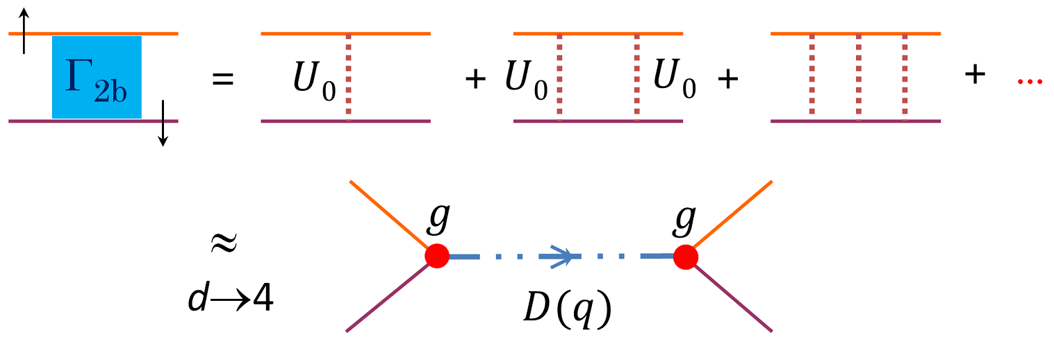
Figure 1: Two fermion scattering in the unitary limit showing the repeated ladder diagrams near four dimensions.

Re-interpretation of the $\epsilon$ expansion. — To calculate the beyond Gaussian contribution, we tie the GPF theory to the dimensional $\epsilon$ expansion by clarifying the structure of the vertex function, $\Gamma(q)$, near four dimensions SupplementalMaterial . We split the normal-state vertex function into its two- and many-body parts, $\Gamma^{-1}(q)=\Gamma_{2b}^{-1}(q)+\Gamma_{mb}^{-1}(q)$, where

$$\Gamma_{2b}^{-1}(q)= \frac{1}{U_{0}}-\sum_{\mathbf{k}}\frac{1}{i\nu_{n}-\varepsilon_{\mathbf{q}}/2-2\epsilon_{\mathbf{k}}-2\mu},$$ (11)

$$\Gamma_{mb}^{-1}(q)= \sum_{\mathbf{k}}\frac{f\left(\xi_{\mathbf{q}/2-\mathbf{k}}\right)+f\left(\xi_{\mathbf{q}/2+\mathbf{k}}\right)}{i\nu_{n}-\varepsilon_{\mathbf{q}}/2-2\varepsilon_{\mathbf{k}}-2\mu}.$$ (12)

For small $\epsilon=4-d$ and in the unitary limit, the two-body part of the vertex function, $\Gamma_{2b}^{-1}(q)$, has a pole and dominates the inverse vertex function,

$$\Gamma_{2b}^{-1} \simeq\frac{m^{2}}{8\pi^{2}\hbar^{4}\epsilon}\left(i\nu_{n}-\varepsilon_{\mathbf{q}}/2+2\mu\right)=\frac{1}{g^{2}D^{2}\left(q\right)},$$ (13)

where we define $g^{2}=(8\pi^{2}\hbar^{4}/m^{2})\epsilon$ and the bosonic propagator, $D(q)=(i\nu_{m}-\varepsilon_{\mathbf{q}}+2\mu)^{-1}$. Thus, we see that the vertex function, $\Gamma(q)$, within the ladder approximation has the leading contribution of $\mathcal{O}(\epsilon)$ near four dimensions in the unitary regime. This is visualized in Fig. 1, where we show the contribution of the two-body scattering near four dimensions.

In the $\epsilon$ expansion, the series is arranged according to orders of $\epsilon$, or equivalently $\Gamma_{2b}$ Nishida2006 . While such an arrangement is convenient to analytically calculate the next-to-leading order (NLO) Nishida2006 or next-to-next-to-leading order (NNLO) of the expansion Arnold2007 , it was known that one may encounter a convergence problem in dealing with some dangerous higher-order terms that contribute like $\mathcal{O}(n!\epsilon^{n})$ due to the exponentially large prefactor $n!$ NishidaAppendixA . These terms are contributions from the many-body part of the vertex function, $\Gamma_{mb}$, to the Gaussian fluctuation part of the thermodynamic potential, $\Omega_{{\rm GF}}^{(2)}$. The summation of these terms is given by, $\sum_{n=1,q}^{\infty}(-1)^{n+1}\left[\Gamma_{2b}\Gamma_{mb}^{-1}\right]^{n}/n=\sum_{q}\ln\left[1+\Gamma_{2b}/\Gamma_{mb}\right]$ SupplementalMaterial , and combining this with the two-body part, $\sum_{q}\ln[-\Gamma_{2b}^{-1}(q)]$, we recover $\Omega_{{\rm GF}}^{(2)}$. Therefore, since $\Omega_{{\rm GF}}^{(2)}$ contains one power of the vertex function, which is $\mathcal{O}(\epsilon)$ at the NLO, the $\epsilon$ expansion can be understood from the framework of the GPF theory. This re-interpretation suggests that it might be more useful to make an expansion in terms of the vertex function, $\Gamma(q)$, instead of $\epsilon$.

Beyond GPF. — As previously noted we have the effective bosonic action, $\mathcal{S}_{{\rm eff}}$, and it is not possible to integrate out the bosonic fluctuations for orders beyond $n=2$ without significant approximations. Using the re-interpretation of the the $\epsilon$-expansion we expand the higher order action terms and use the vertex function as a perturbation parameter, since the higher order contributions to the action will contain multiples of the vertex function and contribute $\mathcal{O}(\epsilon)$ near four dimensions. In these cases we may treat the terms $\mathcal{S}^{(n>2)}$ as perturbative terms with respect to $S_{{\rm GF}}^{(2)}$ and take them into account order by order, using a standard diagrammatic approach. That is, by denoting, $\hat{V}=\mathcal{S}^{(3)}+\mathcal{S}^{(4)}+...,$ we have for the partition function

$$\mathcal{Z} =e^{-\mathcal{S}_{{\rm MF}}^{(0)}}\int\mathcal{D}\left[\Delta,\Delta^{*}\right]e^{-(\mathcal{S}_{{\rm GF}}^{(2)}+\hat{V})}$$

$$=e^{-\mathcal{S}_{{\rm MF}}^{(0)}}\int\mathcal{D}\left[\Delta,\Delta^{*}\right]e^{-\mathcal{S}_{{\rm GF}}^{(2)}}\sum_{n=0}^{\infty}\frac{(-)^{n}}{n!}\left\langle\hat{V}_{1}\hat{V}_{2}\dots\hat{V}_{n}\right\rangle,$$ (14)

where we have inserted a normalization term and defined, for any observable (operator) $\hat{A}$,

$$\left\langle\hat{A}\right\rangle=\frac{\int\mathcal{D}\left[\Delta,\Delta^{*}\right]\hat{A}\,e^{-\mathcal{S}_{{\rm GF}}^{(2)}}}{\int\mathcal{D}\left[\Delta,\Delta^{*}\right]e^{-\mathcal{S}_{{\rm GF}}^{(2)}}}.$$ (15)

Using the linked cluster expansion, we may write,

$$\mathcal{Z}=e^{-\mathcal{S}_{{\rm MF}}^{(0)}}\int\mathcal{D}\left[\Delta,\Delta^{*}\right]e^{-\mathcal{S}_{{\rm GF}}^{(2)}}\exp\left(\sum_{l=1}^{\infty}U_{l}\right),$$ (16)

where the only contribution to the partition function is from the differently-connected diagrams,

$$U_{l}=\frac{(-)^{l+1}}{l}\left\langle\hat{V}_{1}\hat{V}_{2}\dots\hat{V}_{l}\right\rangle_{{\rm dc}}.$$ (17)

The expansion of the thermodynamic potential is then given by,

$$\Omega=\Omega_{{\rm MF}}^{(0)}+\Omega_{{\rm GF}}^{(2)}+\frac{1}{\beta V}\sum_{l=1}^{\infty}\frac{(-)^{l+1}}{l}\left\langle\hat{V}_{1}\hat{V}_{2}\dots\hat{V}_{l}\right\rangle_{{\rm dc}}.$$ (18)

We refer to Supplemental Material for discussions on how to calculate diagrams related to $U_{l}$ SupplementalMaterial . The expansion should converge near four dimensions, where $\Gamma(q)$ is small. Therefore, to select the important diagrams in the calculation of the thermodynamic potential for 3D or 2D, we choose the leading diagrams in orders of $\epsilon$ near four dimensions. Under this guidance, the leading order term beyond GPF is the connected diagram, $\langle{\rm S}^{(4)}\rangle$, which for the normal state is given by,

$$\frac{1}{\beta V}\langle{\rm S}^{(4)}\rangle=\sum_{k}\left[G_{0}(k)\Sigma_{0}(k)\right]^{2},$$ (19)

where the self-energy term is, $\Sigma_{0}(k)=\sum_{q}G_{0}(q-k)\Gamma(q)$ SupplementalMaterial . In the superfluid phase, it takes a more complicated form, $(\beta V)^{-1}\langle{\rm S}^{(4)}\rangle=\Omega^{(a)}+\Omega^{(b)}+\Omega^{(c)}$, where

$$\Omega^{(a)}= \sum_{k}G_{11}^{(0)}(k)G_{11}^{(0)}(k)\Sigma_{11}^{(0)}(k)\Sigma_{11}^{(0)}(k),$$ (20)

$$\Omega^{(b)}= \sum_{k}G_{12}^{(0)}(k)G_{12}^{(0)}(k)\Sigma_{11}^{(0)}(k)\Sigma_{22}^{(0)}(k),$$ (21)

$$\Omega^{(c)}= \sum_{kq_{1}q_{2}}G_{12}^{(0)}(k)G_{11}^{(0)}(k-q_{1})G_{12}^{(0)}(k-q_{1}+q_{2})$$

$$\hskip 21.0ptG_{22}^{(0)}(k+q_{2})\Gamma_{11}(q_{1})\Gamma_{11}(q_{2}),$$ (22)

$\Sigma_{11}^{(0)}(k)=\sum_{k}G_{11}^{(0)}(q-k)\Gamma_{11}^{(0)}(k)$ and $\Sigma_{22}^{(0)}(k)=-\Sigma_{11}^{(0)}(-k)$. As we can see, $\langle{\rm S}^{(4)}\rangle$ contains two $\Gamma(q)$ and near four dimensions is the NNLO, $\mathcal{O}(\epsilon^{2})$ contribution. In other words, if we calculate $\langle{\rm S}^{(4)}\rangle$ in $d=4-\epsilon$ dimensions and numerically extract the coefficients at $\mathcal{O}(\epsilon^{2})$, we are able to recover the NNLO $\epsilon$ expansion Arnold2007 . Higher order $\epsilon$ expansions can be obtained if we go further beyond GPF.

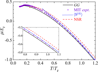
Figure 2: The chemical potential, $\mu/E_{{\rm F}}$, plotted as a function of reduced temperature, $T/T_{{\rm F}}$, found from the MIT experiment (maroon circles) Ku2012 , $GG$ $T$-matrix (black solid) Haussman1994 , NSR (red dashed) Nozieres1985 and $\langle{\rm S}^{(4)}\rangle$ (blue dotted). The inset highlights the high-temperature region for the same figure.

Equation of state. — As an application of our beyond GPF theory, we determine the equation of state of an above threshold strongly interacting Fermi gas in both 3D and 2D, by solving the number equation for the thermodynamic potential, $\Omega=\Omega_{{\rm MF}}^{(0)}+\Omega_{{\rm GF}}^{(2)}+(\beta V)^{-1}\langle{\rm S}^{(4)}\rangle$. Material SupplementalMaterial . We use $\langle{\rm S}^{(4)}\rangle$ as the shorthand notation for our beyond GPF theory in the normal state.

In Fig. 2, we report the chemical potential of a 3D unitary Fermi gas as a function of reduced temperature, $T/T_{{\rm F}}$, predicted from the $\langle{\rm S}^{(4)}\rangle$, ${\rm NSR}$ Nozieres1985 and self-consistent $GG$ theories Haussman1994 , and measured by the MIT experiment Ku2012 . Here, we find that the $\langle{\rm S}^{(4)}\rangle$ prediction is in excellent agreement with the experimental data down to $0.5T_{F}$, below which our prediction begins to diverge away from the ${\rm NSR}$ solution and pairing fluctuations in $\langle{\rm S}^{(4)}\rangle$ start to dominate. This is because, as the temperature becomes lower the effective interaction and fluctuation between pairs become stronger and the NSR approximation itself Liu2006 ; Parish2007 ; Hu2008 , and leading-order correction beyond GPF are no longer controllable.

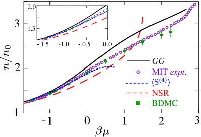
Figure 3: The density equation of state, $n/n_{0}$, plotted as a function of $\beta\mu$, normalized by the ideal gas result, $n_{0}$, at the same temperature $T$ and chemical potential $\mu$, found from the MIT experiment (maroon circles with error bars), $GG$ (black solid), ${\rm NSR}$ (red dashed), $\langle{\rm S}^{(4)}\rangle$ (blue dotted), and bold-diagrammatic QMC (green squares) Houcke2012 . The inset blows up the non-degenerate region for the same plot.

A further comparison is given in Fig. 3, where we plot the density equation of state, $n/n_{0}$, as a function of $\beta\mu$, normalized by the ideal gas result at the same temperature $T$ and chemical potential $\mu$. We find again an excellent agreement between the $\langle{\rm S}^{(4)}\rangle$ prediction and experimental data up to values of $\beta\mu\simeq 0$, as seen clearly in the inset of Fig. 3 for high temperatures. The $\langle{\rm S}^{(4)}\rangle$ prediction agrees well with the experimental data, and shows that our beyond GPF theory is and improvement on $GG$ theory and comparable to bold-diagrammatic QMC Houcke2012 , up to slightly below the Fermi degeneracy. The $\langle{\rm S}^{(4)}\rangle$ theory breaks down at lower temperatures, $\beta\mu\simeq 1$, and as mentioned earlier this is due to the unphysical pair fluctuations dominating as we only calculate the leading term. Our calculations are not stable towards the experimentally measured critical temperature. To understand the superfluid transition using our beyond GPF theory, a below $T_{c}$ calculation with the inclusion of a superfluid order parameter will be implemented and reported later in a more detailed publication.

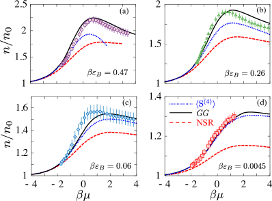
Figure 4: The density equation of state, $n/n_{0}$, normalized by the ideal gas result at the same temperature for the $GG$ (black solid) Bauer2014 ; Mulkerin2015 , ${\rm NSR}$ (red dashed) Marsiglio2015 ; Mulkerin2015 , $\langle{\rm S}^{(4)}\rangle$ and the experimental results Fenech2016 at interaction strengths $\beta\varepsilon_{B}=0.47$, $\beta\varepsilon_{B}=0.26$ , $\beta\varepsilon_{B}=0.06$ and $\beta\varepsilon_{B}=0.0045$.

Encouraged by the excellent agreement between the beyond GPF theory and experiment in 3D, we now turn to consider the density equation of state for a 2D system, where pair fluctuations are believed to become larger. The results are shown in Fig. 4 for the $\langle{\rm S}^{(4)}\rangle$ (blue dotted) and for comparison we plot two theoretical approaches, the NSR (red dashed) Marsiglio2015 ; Mulkerin2015 and $GG$ (black solid) calculation Bauer2014 ; Mulkerin2015 , and the experimental results Fenech2016 for interaction strengths $\beta\varepsilon_{B}=0.47$ (purple circles), $\beta\varepsilon_{B}=0.26$ (green triangles), $\beta\varepsilon_{B}=0.06$ (blue diamonds), and $\beta\varepsilon_{B}=0.0045$ (red squares).

The addition of the higher order terms in the $\langle{\rm S}^{(4)}\rangle$ calculation greatly improves the NSR theory for all interactions and temperatures, and the resulting prediction is comparable to the experimental data and $GG$ calculation up to $\beta\mu\simeq 0$. We can see the $\langle{\rm S}^{(4)}\rangle$ breaking down for low temperatures in Fig. 4(a) and this is due to the fluctuation of pairs becoming more important as in 3D. For the weaker interactions in Figs. 4(c) and 4(d), the inclusion of the $\langle{\rm S}^{(4)}\rangle$ calculation approaches the experimental and $GG$ results.

Conclusions. — We have extended the many-body strong-coupling theory beyond the commonly used Gaussian fluctuation approximation (i.e., the NSR Nozieres1985 or GPF theory Hu2006 ). Inspired by the dimensional expansion near four dimensions Nishida2006 and using the functional path-integral formulation of the thermodynamic potential SadeMelo1993 , we artificially treat a strongly interacting Fermi gas as a system of weakly interacting Cooper pairs and use the vertex function summed over the ladder-type diagrams as a small parameter. This treatment is well justified near four dimensions, where the vertex function is indeed small Nishida2006 . Following this generalization of the dimensional expansion, we re-organize the Feynman diagrams and determine the leading correction term to the Gaussian fluctuations. Applying such a beyond Gaussian fluctuation theory to the three-dimensional strongly interacting unitary Fermi gas in its normal state, we have calculated the equation of state and compared the prediction with the latest experimental data Ku2012 and other theoretical results Nozieres1985 ; Haussman1994 . We have found a sizable improvement on previous many-body calculations down to temperatures of $0.5T_{{\rm F}}$. To further examine the advantage of the theory, we have considered a strongly interacting two-dimensional Fermi gas, for which the pair fluctuations are more significant, and have shown that our theory significantly improves the NSR calculation and captures the high-temperature behavior for strong interactions.

Our theory for the normal state breaks down before the superfluid transition in both 3D and 2D as the NSR theory itself breaks down Liu2006 ; Parish2007 , and we expect that the addition of more terms will lower the temperature range of validity. At zero temperature, where the GPF theory is more reliable Hu2006 ; Diener2008 ; He2015 , we anticipate our theory (i.e., Eqs. (20)-(22)) will provide quantitatively accurate predictions for strongly interacting Fermi gases.

- (1) I. Bloch, J. Dalibard, and W. Zwerger, Rev. Mod. Phys. 80, 885 (2008).
- (2) S. Giorgini, L. P. Pitaevskii, and S. Stringari, Rev. Mod. Phys. 80, 1215 (2008).
- (3) C. Chin, R. Grimm, P. Julienne, and E. Tiesinga, Rev. Mod. Phys. 82, 1225 (2010).
- (4) W. Ketterle and M. W. Zwierlein, Rivista del Nuovo Cimento 31, 247 (2008).
- (5) S. Nascimbène, N. Navon, K. J. Jiang, F. Chevy, and C. Salomon, Nature (London) 463, 1057 (2010).
- (6) M. Horikoshi, S. Nakajima, M. Ueda, and T. Mukaiyama, Science 327, 442 (2010).
- (7) M. J. H. Ku, A. T. Sommer, L. W. Cheuk, and M. W. Zwierlein, Science 335, 563 (2012).
- (8) K. Martiyanov, V. Makhalov, and A. Turlapov, Phys. Rev. Lett. 105, 030404 (2010).
- (9) B. Fröhlich, M. Feld, E. Vogt, M. Koschorreck, W. Zwerger, and M. Köhl, Phys. Rev. Lett. 106, 105301 (2011).
- (10) M. Feld, B. Fröhlich, E. Vogt, M. Koschorreck, and M. Köhl, Nature (London) 480, 75 (2011).
- (11) P. Dyke, E. D. Kuhnle, S. Whitlock, H. Hu, M. Mark, S. Hoinka, M. Lingham, P. Hannaford, and C. J. Vale, Phys. Rev. Lett. 106, 105304 (2011).
- (12) V. Makhalov, K. Martiyanov, and A. Turlapov, Phys. Rev. Lett. 112, 045301 (2014).
- (13) P. A. Murthy, I. Boettcher, L. Bayha, M. Holzmann, D. Kedar, M. Neidig, M. G. Ries, A. N. Wenz, G. Zurn, and S. Jochim, Phys. Rev. Lett. 115, 010401 (2015).
- (14) P. Dyke, K. Fenech, T. Peppler, M. G. Lingham, S. Hoinka, W. Zhang, S.-G. Peng, B. Mulkerin, H. Hu, X.-J. Liu, and C. J. Vale, Phys. Rev. A 93, 011603 (2016).
- (15) I. Boettcher, L. Bayha, D. Kedar, P. A. Murthy, M. Neidig, M. G. Ries, A. N. Wenz, G. Zurn, S. Jochim, and T. Enss, Phys. Rev. Lett. 116, 045303 (2016).
- (16) K. Fenech, P. Dyke, T. Peppler, M. G. Lingham, S. Hoinka, H. Hu, and C. J. Vale, Phys. Rev. Lett. 116, 045302 (2016).
- (17) P. A. Lee, N. Nagaosa, and X.-G. Wen, Rev. Mod. Phys. 78, 17 (2006).
- (18) D. Lee and T. Schfäer, Phys. Rev. C 73, 015201 (2006).
- (19) P. F. Kolb and U. Heinz, in: R. C. Hwa, X.-N. Wang (Eds.), Quark-Gluon Plasma 3, World Scientific, River Edge, NJ, 2004, p. 634.
- (20) X.-W. Guan, M. T. Batchelor, and C. Lee, Rev. Mod. Phys. 85, 1633 (2013).
- (21) X.-J. Liu, H. Hu, and P. D. Drummond, Phys. Rev. Lett. 102, 160401 (2009).
- (22) X. Leyronas, Phys. Rev. A 84, 053633 (2011).
- (23) D. Rakshit, K. M. Daily, and D. Blume, Phys. Rev. A 85, 033634 (2012).
- (24) X.-J. Liu, Phys. Rep. 524, 37 (2013).
- (25) S. Tan, Ann. Phys. 323, 2987 (2008).
- (26) S. Tan, Ann. Phys. 323, 2971 (2008).
- (27) S. Tan, Ann. Phys. 323, 2952 (2008).
- (28) E. Braaten and L. Platter, Phys. Rev. Lett. 100, 205301 (2008).
- (29) G. E. Astrakharchik, J. Boronat, J. Casulleras, S. Giorgini, Phys. Rev. Lett. 93, 200404 (2004).
- (30) A. Bulgac, J. E. Drut, and P. Magierski, Phys. Rev. Lett. 96, 090404 (2006).
- (31) K. V. Houcke, F. Werner, E. Kozik, N. Prokof’ev, B. Svistunov, M. J. H. Ku, A. T. Sommer, L. W. Cheuk, A. Schirotzek, and M. W. Zwierlein, Nature Phys. 8, 366 (2012).
- (32) H. Shi, S. Chiesa, and S. Zhang, Phys. Rev. A 92, 033603 (2015).
- (33) E. R. Anderson and J. E. Drut, Phys. Rev. Lett. 115, 115301 (2015).
- (34) P. Noziéres and S. Schmitt-Rink, J. Low Temp. Phys. 59, 195 (1985).
- (35) C. A. R. Sá de Melo, M. Randeria, and J. R. Engelbrecht, Phys. Rev. Lett. 71, 3202 (1993).
- (36) H. Hu, X.-J. Liu, and P. D. Drummond, Europhys. Lett. 74, 574 (2006).
- (37) X.-J. Liu and H. Hu, Europhys. Lett. 75, 364 (2006).
- (38) M. M. Parish, F. M. Marchetti, A. Lamacraft, and B. D. Simons, Nature Phys. 3, 124 (2007).
- (39) R. B. Diener, R. Sensarma, and M. Randeria, Phys. Rev. A 77, 023626 (2008).
- (40) R. Watanabe, S. Tsuchiya, and Y. Ohashi, Phys. Rev. A 88, 013637 (2013).
- (41) F. Marsiglio, P. Pieri, A. Perali, F. Palestini, and G. C. Strinati, Phys. Rev. B 91, 054509 (2015).
- (42) L. He, H. Lü, G. Cao, H. Hu, and X.-J. Liu, Phys. Rev. A 92, 023620 (2015).
- (43) G. Bighin and L. Salasnich, Phys. Rev. B 93, 014519 (2016).
- (44) H. Hu, X.-J. Liu, and P. D. Drummond, Phys. Rev. A 77, 061605(R) (2008).
- (45) H. Hu, X.-J. Liu, and P. D. Drummond, New J. Phys. 12, 063038 (2010).
- (46) B. C. Mulkerin, K. Fenech, P. Dyke, C. J. Vale, X.-J. Liu, and H. Hu, Phys. Rev. A 92, 063636 (2015).
- (47) Q. Chen, J. Stajic, S. Tan, and K. Levin, Phys. Rep. 412, 1 (2005).
- (48) R. Haussman, Phys. Rev. B 49, 12975 (1994).
- (49) X.-J. Liu and H. Hu, Phys. Rev. A 72, 063613 (2005).
- (50) R. Haussmann, W. Rantner, S. Cerrito, and W. Zwerger, Phys. Rev. A 75, 023610 (2007).
- (51) M. Bauer, M. M. Parish, and T. Enss, Phys. Rev. Lett. 112, 135302 (2014).
- (52) Y. Nishida, Unitary Fermi gas in the expansion, PhD thesis, Univeristy of Tokyo (2006); arXiv:cond-mat/0703465.
- (53) Y. Nishida and D. T. Son, Phys. Rev. Lett. 97, 050403 (2006).
- (54) Y. Nishida and D. T. Son, Phys. Rev. A 75, 063617 (2007).
- (55) Y. Nishida, Phys. Rev. A 75, 063618 (2007).
- (56) P. Arnold, J. E. Drut, and D. T. Son, Phys. Rev. A 75, 043605 (2007).
- (57) Z. Nussinov and S. Nussinov, Phys. Rev. A 74, 053622 (2006).
- (58) K. B. Gubbels and H. T. C. Stoof, Phys. Rev. A 84, 013610 (2011).
- (59) More details can be found in Supplemental Material, which outlines the relation between the expansion and the GPF theory, Feynman diagram rules, and our numerical procedure.
- (60) Please refer to Appendix A of the reference NishidaPhDThesis .