Capturing the Dynamical Repertoire of Single Neurons with Generalized Linear Models

Alison I. Weber${}^{\text{1}}$ & Jonathan W. Pillow${}^{\text{2},\text{3}}$
${}^{\text{1}}$Graduate Program in Neuroscience, University of Washington, Seattle, WA, USA.
${}^{\text{2}}$Princeton Neuroscience Institute, Princeton University, Princeton, NJ, USA.
${}^{\text{3}}$Dept. of Psychology, Princeton University, Princeton, NJ, USA.

Keywords: point process; generalized linear model (GLM); Izhikevich model; spike timing; variability

A key problem in computational neuroscience is to find simple, tractable models that are nevertheless flexible enough to capture the response properties of real neurons. Here we examine the capabilities of recurrent point process models known as Poisson generalized linear models (GLMs). These models are defined by a set of linear filters, a point nonlinearity, and conditionally Poisson spiking. They have desirable statistical properties for fitting and have been widely used to analyze spike trains from electrophysiological recordings. However, the dynamical repertoire of GLMs has not been systematically compared to that of real neurons. Here we show that GLMs can reproduce a comprehensive suite of canonical neural response behaviors, including tonic and phasic spiking, bursting, spike rate adaptation, type I and type II excitation, and two forms of bistability. GLMs can also capture stimulus-dependent changes in spike timing precision and reliability that mimic those observed in real neurons, and can exhibit varying degrees of stochasticity, from virtually deterministic responses to greater-than-Poisson variability. These results show that Poisson GLMs can exhibit a wide range of dynamic spiking behaviors found in real neurons, making them well suited for qualitative dynamical as well as quantitative statistical studies of single-neuron and population response properties.

1 Introduction

Understanding the dynamical and computational properties of neurons is a fundamental challenge in cellular and systems neuroscience. A wide variety of single-neuron models have been proposed to account for neural response properties. These models can be arranged along a complexity axis ranging from detailed, interpretable, biophysically accurate models to simple, tractable, reduced functional models. Detailed Hodgkin-Huxley style models, which sit at one end of this continuum, provide a biophysically detailed account of the conductances, currents, and channel kinetics governing neural response properties [21]. These models can account for the vast dynamical repertoire of real neurons, but they are often unwieldy for theoretical analyses of neural coding and computation. This motivates the need for simplified models of neural spike responses that are tractable enough for mathematical, computational, and statistical analyses.

A variety of simplified dynamical models have been proposed to serve the need for mathematically tractable models, including the integrate-and-fire model, Fitzhugh-Nagumo, Morris-Lecar, and Izhikevich models [9, 33, 32, 22, 4]. Generally, these models aim to reduce the biophysically detailed descriptions of realistic neurons to systems of differential equations with fewer variables and/or simplified dynamics. The one-dimensional integrate-and-fire model is arguably the simplest of these, and the simplest to analyze mathematically, but it fails to capture many of the response properties of real neurons. The two-dimensional Izhikevich model, by contrast, was specifically formulated to retain the rich dynamical repertoire of more complex, biophysically realistic models [23].

An alternative to a mathematical notion of simplicity is the statistical property of being tractable for fitting from intracellular or extracellular physiological recordings. One well-known statistical model that satisfies this desideratum is the recurrent linear-nonlinear Poisson model, commonly referred to in the neuroscience literature as the generalized linear model (GLM) [48, 40]. GLMs are closely related to generalized integrate-and-fire models such as the spike-response model, which has linear dynamics but incorporates spike-dependent feedback to capture the nonlinear effects of spiking on neural membrane potential and subsequent spike generation [13, 26, 24, 39, 16]. In fact, a variant of the spike response model that incorporates noise into the spike threshold is mathematically equivalent to the models we study here [15, 12, 25, 14]. GLMs are popular for characterizing neural responses in reverse-correlation or white-noise experiments, due to the tractability of likelihood-based fitting methods. Recent work has shown that GLMs can capture the detailed statistics of spiking in single and multi-neuron recordings from a variety of brain areas [40, 2, 5, 50, 31, 41].

While several studies have shown that GLMs can successfully recapitulate various response properties of biological or simulated neurons, here, we provide a more systematic study of the dynamical repertoire of the GLM . We study this issue by fitting GLMs to data from simulated neurons exhibiting a number of complex response properties. We show that GLMs can reproduce a remarkably rich set of dynamical behaviors, including tonic and phasic spiking, bursting, spike rate adaptation, type I and type II excitation, and two different forms of bistability. Furthermore, GLMs can exhibit stimulus-dependent degrees of spike timing precision and reliability [29], and mimic a recently reported form of greater-than-Poisson variability [17].

2 Models of dynamical behaviors

2.1 Izhikevich model

First, we will examine whether generalized linear models can reproduce a suite of canonical spiking behaviors exhibited by the well-known Izhikevich model [22, 23]. The Izhikevich model is a biophysically-inspired model of intracellular membrane potential defined by a two-variable system of ordinary differential equations governing membrane potential $v(t)$ and a recovery variable $u(t)$:

$$\dot{v}=0.04v^{2}+5v+140-u+I(t)$$ (1)

$$\dot{u}=a(bv-u)$$ (2)

with spiking and voltage-reset governed by the boundary condition:

$$\text{if }v(t)\geq 30,\;\text{``spike'' and set}\left\{\begin{array}[]{ll}v(t^{+})=c\\ u(t^{+})=u(t)+d,\end{array}\right.$$ (3)

where $I(t)$ is injected current, $t^{+}$ denotes the next time step after $t$, and parameters $(a,b,c,d)$ determine the model’s dynamics. Different settings of these parameters lead to qualitatively different spiking behaviors, as shown in [23]. We focus on this model because of its demonstrated ability to produce a wide range of response properties exhibited by real neurons. (See Table 1 for parameter values used in this study and Methods for simulation details.)

2.2 Generalized linear model (GLM)

The GLM is a regression model typically used to characterize the relationship between external or internal covariates and a set of recorded spike trains. In systems neuroscience, the label “GLM” often refers to an autoregressive point process model, a model in which linear functions of stimulus and spike history are nonlinearly transformed to produce the spike rate or conditional intensity of a Poisson process [48, 40].

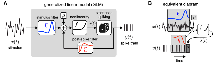
Figure 1: Schematic of the generalized linear model. A: The stimulus filter $\vec{k}$ operates linearly on the stimulus $x(t)$, is combined with input from the post-spike filter $\vec{h}$ and mean input level $\mu$. This combined linear signal passes through a point nonlinearity $f(\cdot)$, whose output drives spiking via a conditionally Poisson process. B: An equivalent view of the GLM, which emphasizes the dependencies between a particular time window of stimulus and spike history and conditional intensity $\lambda(t)$, which governs the probability of a spike in the current time bin (dark gray box).

The GLM is parametrized by a stimulus filter $\vec{k}$, which describes how the neuron integrates an external stimulus, a post-spike filter $\vec{h}$, which captures the influence of spike history on the current probability of spiking, and a scalar $\mu$ that determines the baseline spike rate. (See Figure 1.) The outputs of these filters are summed and passed through a nonlinear function $f$ to determine the conditional intensity $\lambda(t)$:

$$\lambda(t)=f(\vec{k}\cdot\vec{x}(t)\;+\;\vec{h}\cdot\vec{y}_{hist}\left(t\right)\;+\;\mu),$$ (4)

where $\vec{x}(t)$ is the (vectorized) spatio-temporal stimulus, $\vec{y}_{hist}(t)$ is a vector representing spike history at time $t$, and $f$ is a nonlinear function that ensures the spike rate is non-negative. Spikes are generated according to a conditionally Poisson process [37, 6], so spike count $y(t)$ in a time bin of size $\Delta$ is distributed according to a Poisson distribution:

$$P(y(t)|\lambda(t))=\frac{1}{y(t)!}\Big{(}\Delta\lambda(t)\Big{)}^{y(t)}e^{-\Delta\lambda(t)}.$$ (5)

In this study we set $f$ to be exponential, although similar properties can be obtained with other nonlinearities such as the soft-rectification function.

Unlike classical deterministic models like Hodgkin-Huxley and integrate-and-fire, the GLM is fundamentally stochastic due to the assumption of conditionally Poisson spiking. However, this stochasticity is helpful for fitting purposes because it assigns graded probabilities to firing events and allows for likelihood-based methods for parameter fitting [35, 39]. In fact, the Poisson GLM comes with a well-known guarantee that the log-likelihood function is concave for suitable choices of nonlinearity $f$ [34]. This means we can be assured of approaching a global optimum of the likelihood function via gradient ascent, for any set of stimuli and spike trains (barring any numerical issues that may complicate achieving the actual maximum for certain datasets, cf. [53]). This guarantee does not hold for stochastic formulations of most nonlinear biophysical models, including the Izhikevich model. Moreover, despite its stochasticity, the GLM can produce highly precise and repeatable spike trains in certain parameter settings, as we will demonstrate below.

3 GLMs capture a wide array of complex dynamical behaviors

We fit GLMs to data simulated from Izhikevich neurons set up to exhibit a range of different qualitative response behaviors. In the following, we describe these behaviors in detail, beginning with simpler behaviors, such as tonic spiking and bursting (which have already been demonstrated in previous work, e.g., [15, 25]) in order to build intuition for the GLM’s basic capabilities, and then move on to more complex behaviors (such as bistability) and questions of spike timing reliability and precision.

3.1 Tonic spiking

We first examined an Izhikevich neuron tuned to exhibit tonic spiking (Figure 2A-B; see Table 1 for parameters). When presented with a step input current, the Izhikevich neuron responds with a few high-frequency spikes and then settles into a regular firing pattern that persists for the duration of the step (Figure 2B). This response pattern resembles that of a deterministic Hodgkin-Huxley or integrate-and-fire neuron, albeit with an added transient burst of spikes at stimulus onset.

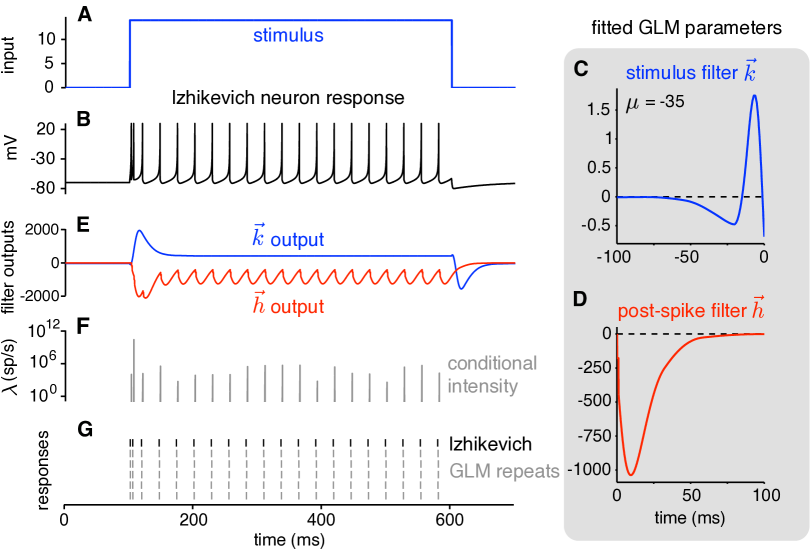
Figure 2: Tonic spiking behavior. A: A step current stimulus. B: Voltage response of the simulated Izhikevich neuron. C: The fitted GLM stimulus filter $\vec{k}$ has a biphasic shape that gives the model a vigorous response to stimulus onset and a net positive response to a sustained input. D: The fitted GLM post-spike filter $\vec{h}$ has a negative lobe that imposes strong refractoriness on a timescale of $\approx$50 ms. E: Stimulus (blue) and post-spike (red) filter outputs during simulated response of the fitted GLM to the stimulus shown above on a single trial. F: The summed filter outputs are passed through an exponential nonlinearity to determine the conditional intensity $\lambda(t)$, shown here for a single trial. G: Spike train of the Izhikevich neuron (black) and simulated repeats of the GLM (gray). GLM spike responses are slightly different on each trial, due to the stochasticity of spike generation, but reproduce Izhikevich model spike times with high precision.

We simulated the Izhikevich neuron’s response to a series of step currents and used the resulting training data to perform maximum-likelihood fitting of the GLM parameters $\{\vec{k},\vec{h},\mu\}$. The estimated stimulus filter $\vec{k}$ is biphasic (Figure 2C), resulting in a large transient response to stimulus onset, and has a positive integral, ensuring a sustained positive response to a current step (Figure 2E, blue trace). The estimated post-spike filter $\vec{h}$ (Figure 2D), by contrast, has a large negative lobe that provides recurrent inhibition after every spike, enforcing a strong relative refractory period. The stimulus filter and post-spike filter output (shown together for a single trial in Figure 2E) are summed together and exponentiated to obtain the conditional intensity $\lambda(t)$ (Figure 2F), also known as the instantaneous spike rate.

For this stimulus, the intensity rises very quickly once $\vec{h}$ decays, which occurs approximately 50 ms after the previous spike. Note that the output of the stimulus filter is identical on each trial, whereas the the output of the post-spike filter varies from trial to trial because of variability in the exact timing of spikes. However, because the rising phase of the conditional intensity is so rapid, spiking is virtually certain within a small time window sitting at a fixed latency after the previous spike time. The combination of strong excitatory drive from the stimulus filter and strong suppressive drive from the post-spike filter produces precisely timed spikes across trials, allowing the GLM to closely match the deterministic firing pattern of the Izhikevich neuron (Figure 2G).

3.2 Bursting

We next examined multi-spike bursting, a more complex temporal response pattern that requires dependencies beyond the most recent interspike interval.

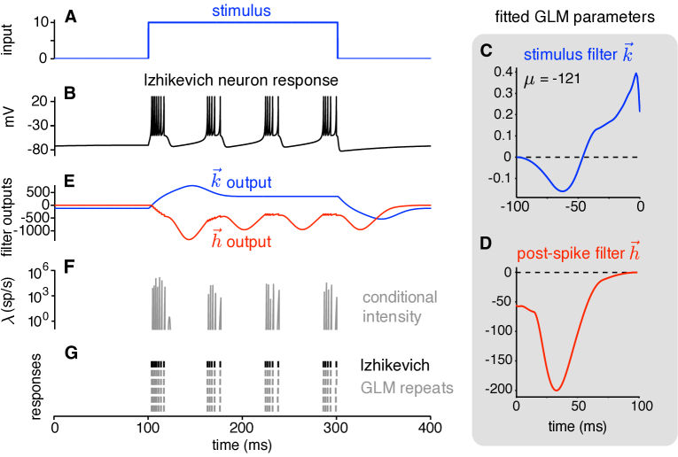
Figure 3: Bursting behavior. A: Step current stimulus. B: Voltage response of Izhikevich neuron. C: Fitted GLM stimulus filter. D: Fitted GLM post-spike filter, which creates refractoriness on short timescales (within each burst) due to instantaneous depolarization following a spike. The large negative lobe $\approx$25-50 ms after a spike terminates bursting and strongly suppresses firing between bursts. E: Stimulus (blue) and post-spike (red) filter outputs for simulated response of the GLM to step current shown above on a single trial. F: Output of the nonlinearity (conditional intensity) $\lambda(t)$ on a single trial. G: Spike train of Izhikevich neuron (black) and simulated repeats of the fitted GLM (gray).

Once again, we simulated responses from an Izhikevich neuron tuned to exhibit tonic bursting (Figure 3A-B) and used the resulting data to fit GLM parameters (Figure 3C-D). The estimated stimulus filter $\vec{k}$ is biphasic with a larger positive than negative lobe, which drives rapid spiking at stimulus onset and generates sustained drive during an elevated stimulus (Figure 3E, blue trace). The post-spike filter $\vec{h}$ has an immediate negative component that creates a relative refractory period after each spike, and an even more negative mode after a latency of $\approx$40 ms; the accumulation of these negative components over multiple spikes gives rise to a sustained suppression of activity between bursts.

The GLM captures the bursting behavior of the Izhikevich neuron with high precision, including the fact that the first burst after stimulus onset contains a different pattern of spikes than subsequent bursts. This difference arises from precise interactions between the stimulus and post-spike filter outputs. During the first burst, fast spiking arises from an interplay between monotonically increasing stimulus filter output (Figure 3E, blue) and tonic decrements induced by the post-spike filter after each spike (Figure 3E, red). After each spike, the post-spike filter reduces the conditional intensity by a fixed decrement, but this decrement is soon overwhelmed by the rising wave of input from the stimulus filter, which creates a rapid rise and fall of the conditional intensity time-locked to each Izhikevich neuron spike time. The pattern continues until accumulated contributions from the delayed negative lobes of post-spike filter overwhelm those from the stimulus filter and the burst terminates. Subsequent bursts are governed by a somewhat different interplay between stimulus and post-spike filter outputs: bursts sit on a rising phase of the conditional intensity due to the removal of suppression from the previous burst. This rise is more gradual than the drive induced by stimulus onset, and results in bursts with longer inter-spike intervals and fewer spikes per burst, but the resulting spike pattern is nonetheless captured with high precision and reliability from trial to trial.

3.3 Bistability

Bistability refers to the phenomenon in which there are multiple stable response modes for a single input condition. A common form of bistability observed in real neurons is the ability to inhabit either a tonically active state or a silent state for a given level of current injection. The Izhikevich model can exhibit this form of bistability, wherein a brief positive current pulse is sufficient to kick it between states: the neuron can inhabit a silent state in the absence of stimulation, but a brief positive current pulse kicks it into a tonically active state, and an appropriately-timed positive pulse kicks it back to the silent state (Figure 4A-B).

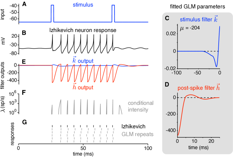
Figure 4: Bistable responses. A: Stimulus consisting of two brief positive current pulses. B: Voltage response of Izhikevich neuron, which exhibits bistability. The first pulse initiates a tonic spiking mode and the second pulse (precisely timed to the phase of the spike response) terminates it, returning to a quiescent mode. C: Fitted GLM stimulus filter, which provides a biphasic impulse response. D: Fitted post-spike filter, which imposes a refractory period of $\approx$4 ms and gives increased probability of firing $\approx$5-10 ms after each spike. E: GLM stimulus (blue) and post-spike (red) filter outputs on a single trial. F: Output of the nonlinearity gives the conditional intensity for a single trial. G: Spike train of Izhikevich neuron (black) and simulated repeats of the fitted GLM (gray).

We fit a GLM to spike trains simulated from such a bistable Izhikevich neuron and found that the fitted GLM can capture bistable behavior of the original model with high accuracy (Figure 4C-G). When stimulated during the silent state, the GLM emits a spike due to the positive output of the stimulus filter (Figure 4E, blue), and tonic firing ensues due to a positive lobe in the post-spike filter that causes self-excitation at a fixed latency of approximately 10 ms after the previous spike (Figure 4E). The GLM returns from the active state to the silent state when a positive stimulus pulse synchronizes negative lobes of the stimulus and post-spike filters. Only the combination of these two negative drives is strong enough to shut off spiking; without the negative drive created by previous spikes (appearing in the post-spike filter at a latency of 15 ms after a spike), suppression from the negative lobe of the stimulus filter is not strong enough to prevent spiking. As with the tonic spiking neuron discussed above, the interaction between the stimulus and post-spike filters generates rapid rises in the conditional intensity (Figure 4F), leading to precisely timed spikes that mimic those of the deterministic Izhikevich neuron (Figure 4G).

This Izhikevich neuron (with the same parameters) can also exhibit a second form of bistability, in which the return to the silent state from the active state is induced by a negative instead of a positive current pulse. We performed a similar fitting exercise and found that the GLM is also able to reproduce this behavior. Firing is initiated and maintained by a similar mechanism as the first form of bistability, but firing offset occurs due to the fact that a negative stimulus pulse creates immediate negative output from the stimulus filter, which suppresses firing during the time when a spike would have occurred due to spike-history filter input. Tonic firing is extinguished more rapidly in this second form of bistability than the first (see Figure 6 below).

3.4 Type I and type II firing

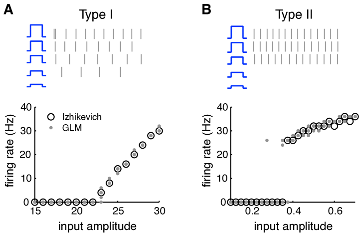
Figure 5: Type I and type II firing curves. A: Top: Example responses of a GLM exhibiting type I firing behavior. The spike rate increases continuously from zero in response to current steps of increasing amplitude. Bottom: F-I curve for a type I Izhikevich neuron (black) and corresponding GLM (gray). For the GLM, responses are plotted for five repetitions of each input amplitude. B: Similar plots for type II firing behavior, characterized by a discontinuous jump from zero to a finite spike rate in responses to current steps of increasing amplitude.

Neurons have been classified as exhibiting either type I or type II dynamics based on the shape of their firing rate vs. intensity (F-I) curve. Type I neurons can fire at arbitrarily low rates for low levels of injected current, whereas type II neurons have discontinuous F-I curves that arise from an abrupt transition from silence to a finite non-zero firing rate as the level of injected current increases [20]. We simulated Izhikevich neurons that exhibit each of these response types using published parameters. Inputs consisted of 500 ms current steps of varying amplitude. The resulting F-I curves for the Izhikevich type I and type II neurons are shown in black in Figure 5A and Figure 5B, respectively. We fit GLMs using data from each Izhikevich neuron and found that the fitted GLMs capture the two response types with high temporal precision. The corresponding F-I curves are shown in gray in Figure 5 and accurately mimic the behaviors of the Izhikevich neuron. Similar F-I curves have been demonstrated previously in [15] and [31].

The only discrepancy between the Izhikevich and GLM neurons occurs for the type II cell at input amplitudes near the Izhikevich neuron’s threshold. On some trials when the input amplitude falls below this threshold, the GLM jumps into a a tonic firing state for the duration of the stimulus. Similarly, on some trials when the input amplitude falls above this threshold, the GLM fails to initiate firing. This is unsurprising given the stochastic nature of the GLM. Importantly, the GLM never fires at a low rate, but rather abruptly transitions from no firing to firing at a baseline level of $\approx$25 Hz, reflecting type II behavior.

3.5 Additional behaviors

We fit GLMs to every dynamical behavior considered in [23] with the exception of purely subthreshold behaviors, since GLM fitting uses spike trains and does not consider sub-threshold responses. The full suite of behaviors is shown in Figure 6, with responses of the Izhikevich neurons in black and spike responses of the GLM in gray. This list includes tonic and phasic spiking, tonic and phasic bursting, mixed mode firing, spike frequency adaptation, type I and type II excitability, two different forms of bistability, and several others that depend primarily on the shape of stimulus filter. Several additional behaviors that can be captured by a GLM are not depicted in Figure 6 as they can be achieved by a trivial manipulation of the stimulus filter; for example, inhibition-induced bursting can be achieved by simply flipping the sign of the stimulus filter for the bursting neuron shown in Figure 6C. Previous work has shown the Izhikevich neuron to be capable of producing 18 distinct spiking behaviors [23], and we found that all can also be produced by a GLM.

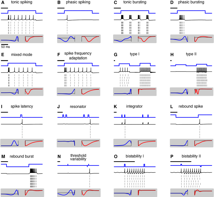
Figure 6: Suite of dynamical behaviors of Izhikevich and GLM neurons. Each panel, top to bottom: stimulus (blue), Izhikevich neuron response (black), GLM responses on five trials (gray), stimulus filter (left, blue), and post-spike filter (right, red). Black line in each plot indicates a 50 ms scale bar for the stimulus and spike response. (Differing timescales reflect timescales used for each behavior in original Izhikevich paper [23]). Stimulus filter and post-spike filter plots all have 100 ms duration.

3.6 Systematic variation of filter amplitudes

We next considered what happens to the behaviors produced by a GLM as some aspect of the filters is systematically varied. To do so, we created stimulus and post-spike filters composed by linear combinations of two basis filters, and then systematically varied the amplitude of one basis filter while holding the other fixed. (See Methods for details.) Figure 7 shows the phase space of qualitative spiking behaviors obtained at different points in this 2D filter space.

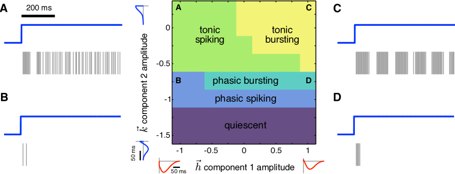
Figure 7: Changes in a single component of each filter can produce a variety of behaviors. Center: Amplitudes for a single component of the stimulus filter (ordinate) or post-spike filter (abscissa) were varied. Responses were simulated for 15 trials of a step stimulus, and the most common behavior produced is indicated by color. Small panels show example filters at each extreme of the range tested. A-D: Example responses (gray) to step stimulus (blue) for GLMs with filters indicated by corresponding letter in center panel.

When the stimulus filter has a strongly negative component (center panel, bottom), a positive stimulus pulse does not produce enough driving force to cause the neuron to spike at all (quiescent). As the amplitude of this component of the stimulus filter is increased, the neuron receives stronger and stronger input and is driven first to spike once or twice (phasic spiking), and eventually to emit a burst of spikes (phasic bursting). The stimulus filter largely drives changes between these behaviors, with the additional detail that a strongly negative post-spike filter component is able to inhibit a burst that would otherwise occur (upper left corner of “phasic spiking" region). As the stimulus filter component becomes still more positive and the stimulus filter transitions from being biphasic to more monophasic, it produces a positive driving force for the duration of the stimulus step, rather than just the onset. This causes the neuron to fire for the duration of the step.

Importantly, the post-spike filter here determines the nature of this sustained firing. A post-spike filter that is purely negative beginning at short timescales (top, left side) mimics a relative refractory period, inhibiting additional spikes for a short window following each elicited spike and resulting in tonic spiking. If, on the other hand, the post-spike filter is only weakly negative at short timescales while being more strongly negative at longer timescales, this creates multiple timescales in the neuron’s response (top, right side). At short timescales, there is little inhibition from each spike (beyond the absolute refractory period), so additional spikes may occur. Over longer timescales, inhibition is accumulated over multiple spikes, which eventually shuts off spiking. After a brief window of no spikes, the inhibition is relaxed and spiking commences again until enough inhibition is accumulated to shut spiking off. This cycle results in tonic bursting for the duration of the step. In the extreme case where the post-spike filter is actually biphasic (top, far right), each spike promotes additional spikes on short timescales, leading to highly regular timing of spikes within bursts (Figure 7C). This set of behaviors could be achieved by simply sweeping over the amplitude of a single basis vector in each filter. Incorporating shifts to the basis vectors or additional basis vectors would likely be necessary to achieve more complex behaviors, such as bistability.

Although we have drawn clear borders at the transition between behaviors, these transitions in fact occur gradually. Near the border between phasic spiking and phasic bursting, for example, there will be some trials where a single spike is produced and other trials where a burst is elicited. We have indicated the behavior that is produced most frequently here for simplicity. The transition from tonic bursting to tonic spiking also occurs gradually, with the near perfectly regular bursting breaking down into more irregular firing until no apparent bursts are produced. If the post-spike filter is made even more negative than the range explored in this figure, the timing of tonic spiking becomes near perfectly regular as well. This is easily explained by the fact that as the post-spike filter becomes more and more negative, it imposes stronger refractoriness on the cell, which results in more regular spike timing. As the post-spike filter component amplitude is changed, there is therefore a gradual change from precisely timed bursts, to irregular firing, to precisely timed tonic spiking. In the following section, we further explore questions of spike timing precision in the GLM.

3.7 Generalization to new stimuli

[capbesideposition=right,top,capbesidewidth=5cm]figure[]

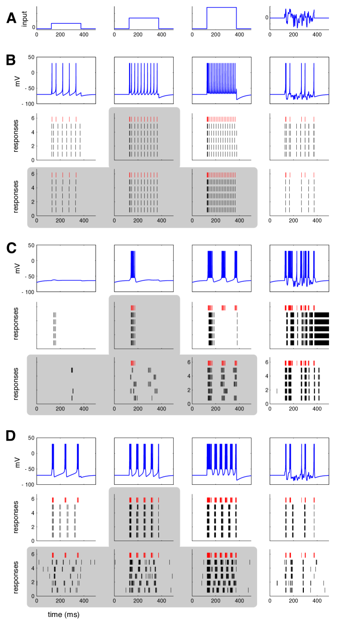
Figure 8: GLMs have limited ability to genearlize to new stimuli. A: Inputs used to generate responses from Izhikevich neurons. Step amplitudes were 7, 14, & 28; 0.3, 0.6, & 1.2; and 5, 10, & 20 for B, C, & D, respectively. Standard deviation of noise was 7.2 for all neuron types. B: Top: Responses of a regular spiking Izhikevich neuron to the above stimuli. Middle: Spike responses of the Izhikevich neuron (red) and GLM (black) fit on responses to only the middle step size (indicated by gray box). Bottom: Spike responses of the Izhikevich neuron (red) and GLM (black) fit on responses to all three step sizes (indicated by gray box). C: Responses of a phasic bursting Izhikevich neuron. All panels as in B. D: Responses of a tonic bursting Izhikevich neuron. All panels as in B & C.

The behaviors shows in Figure 6 were all fit using stimuli that probe only a small range of the possible behaviors of the neuron. For example, many were probed using only a single step height. A natural question that arises is therefore: how well will these fitted GLMs generalize to predict the Izhikevich neuron responses to new stimuli? We examined this question for three canonical Izhikevich neurons from our study (Figure 8). We first generated responses from a regular spiking Izhikevich neuron using three step heights and one noise stimulus (Figure 8A; B, top). We then simulated responses to these stimuli using the GLM fit only to the intermediate step height (Figure 8B, middle). (This is the same fit as Figure 2.) The GLM responses nearly perfectly capture the Izhikevich responses for the original stimulus, and the GLM maintains regular firing patterns for the other step heights. However, the GLM’s firing rate is too high for the small step and too low for the large step. While the GLM accurately captures some firing events for the noise stimulus, the firing rate is overall too high. We next refit a GLM to responses from all three step heights, using the same set of basis vectors as the original fit (Figure 8, bottom). The responses to all three step heights are captured nearly perfectly. Additionally, the response to the noise stimulus is much more similar to that of the Izhikevich neuron. Although there is one firing event that occurs at a delay, the regular spiking GLM fit on an enriched stimulus set is better able to generalize to the noise stimulus.

We performed this same test for neurons showing phasic bursting (Figure 8C) and tonic bursting (Figure 8D). (Note that although some responses of the phasic bursting Izhikevich neuron are not actually phasic, we retain the naming convention given to this set of parameters in the original paper.) For phasic bursting, the GLM fit on additional step sizes improves the accuracy of responses to the smallest and largest steps, while decreasing the accuracy of responses for the original step of intermediate size. There is marked improvement in the accuracy of responses to the noise stimulus, with many firing events being accurately captured and the GLM no longer exhibiting runaway excitation. For tonic bursting, the refit GLM retains bursting behavior but fails to even capture responses for the steps on which it was trained. As noted above, when refitting we used the same set of basis vectors as the initial fits for fair comparison. It is possible that by increasing the number of basis vectors used or tuning their properties that better fits to all stimuli might be achieved.

Taken together, these results show that while GLMs might retain some characteristic response features (such as bursting) when probed with new stimuli, they often have limited ability to generalize beyond stimuli on which they are directly fit.

4 Spiking precision and reliability

A noteworthy feature of the spike trains of the GLM neurons considered above is their high degree of spike timing precision and reliability across trials. This precision arises from the fact that the conditional intensity (or instantaneous spike rate) rises abruptly at spike times (due to filter outputs passing through a rapidly accelerating exponential nonlinearity), and decreases immediately after each spike due to suppressive effects of the post-spike filter. By contrast, a Poisson GLM without recurrent feedback, more commonly known as a linear-nonlinear Poisson (LNP) cascade model, cannot produce temporally precise spike responses to a constant stimulus because its output is constrained to be a Poisson process.

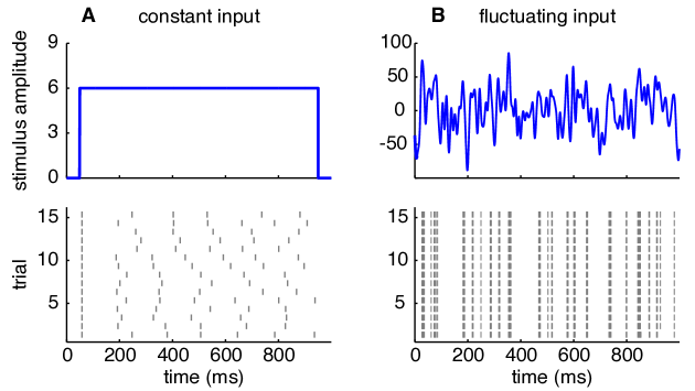
Figure 9: Stimulus-dependent spike timing reliability. A: Top: Weak step stimulus. Bottom: Spike train responses of tonic-spiking GLM on 15 repeated trials. Although the first spike is precise and reliable, subsequent spikes have irregular timing from trial to trial. B: Top: Rapidly fluctuating stimulus. Bottom: Spike response of same GLM neuron on 15 repeated trials, exhibiting a high degree of precision and reliability. (Compare to Figure 1 of [29].)

Real neurons, however, seem to be capable of both response modes: they emit precisely-timed spikes in some settings and highly variable spike trains in others. A seminal paper by Mainen & Sejnowski illustrated this duality by showing that spike responses to a constant DC current exhibit substantial trial-to-trial variability, whereas responses to a rapidly fluctuating injected current are precise and repeatable across trials [29]. Deterministic models like the Izhikevich model cannot, of course, mimic this property because their spikes are perfectly reproducible for any stimulus. (A stochastic version of the Izhikevich model with an appropriate level of injected noise could likely overcome this shortcoming, however. See [44] for a similar case in a Hodgkin-Huxley neuron.) Here we show that the GLM naturally reproduces the same form of stimulus-dependent changes in precision and reliability observed in real neurons. Figure 9 shows that a single GLM (with parameters identical to those fit to the tonic-spiking Izhikevich neuron, shown in Figure 2) produces irregular spiking in response to a constant stimulus with low-to-intermediate amplitude, and precisely-timed, reliable spikes in response to a stimulus with large, rapid fluctuations.

5 GLMs can produce super-Poisson variability

We have shown that GLM neurons can reproduce the high degree of spike timing precision found in real neurons stimulated with injected currents. However, a variety of studies have reported that neurons exhibit overdispersed responses, or greater-than-Poisson spike count variability in response to repeated presentations of a sensory stimulus [47, 46, 45, 17]. A prominent recent study from Goris, Movshon, & Simoncelli showed that the degree of overdispersion grows with mean spike count, so that the Fano factor (variance-to-mean ratio) is an increasing function of spike rate [17]. They proposed a doubly stochastic model to account for this phenomenon, in which the rate of a Poisson process is modulated by a slowly fluctuating stochastic gain variable $g$. For each trial, $g$ is drawn from a gamma distribution with mean 1 and variance $\sigma_{g}^{2}$. (See Methods for details.)

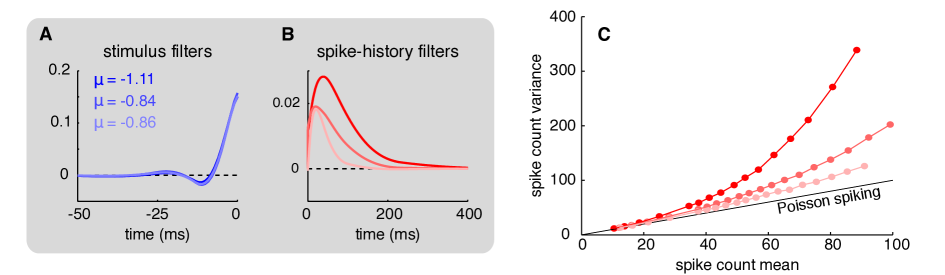
Figure 10: GLMs can produce super-Poisson variability. A: Stimulus filters for GLMs trained on three different levels of variability: high (dark blue), medium (medium), and low (light) super-Poisson variability. Spike count mean was identical in the three cases: 100 spikes/s. B: Post-spike filters for high (dark red), medium (medium), and low (light) super-Poisson variability. C: Spike count variance versus mean for three levels of variability. This relationship is strikingly similar to that observed in many cortical neurons.

We sought to determine if a GLM with spike-history dependence can also account for the mean-dependent overdispersion found in neural responses. To test this possibility, we simulated spike trains from the doubly stochastic model of Goris et al for three different settings of the over-dispersion factor $\sigma_{g}^{2}$ with the same mean spike rate (100 spikes/s), and fit a GLM to the spike trains associated with each value of $\sigma_{g}^{2}$. We then simulated responses from each GLM to 500 ms pulses at a number of different input intensities, with each point in Figure 10 corresponding to a different intensity.

We found that the GLM can indeed match the qualitative behavior of the Goris et al model, giving approximately Poisson responses at low spike rates and increasingly overdispersed responses at higher rates (Figure 10C). To match the data from larger values of overdispersion factor $\sigma_{g}^{2}$ (darker curves in Figure 10C), the GLM relies on increasing amounts of self-excitation from the post-spike filter, but exhibits no changes in stimulus filter (Figure 10A-B). The filters here do not include an absolute refractory period, as the original model does not incorporate one. However, similar results can be achieved when a refractory period is enforced in the training data. This will result in post-spike filters with strongly negative lobes on short timescales, which impose refractoriness, but otherwise similar filters to those in Figure 10. Unlike models with purely suppressive spike history effects, which capture effects due to refractoriness and reduce variability in firing (e.g., [3, 49]), here we show that allowing spike history effects to be excitatory can result in increased variability. While the former might be suitable for early sensory areas, such as the retina, the latter better captures the super-Poisson variability observed in higher visual areas.

Intuitively, the GLM generates overdispersed spike counts because of dependencies the spike-history filter induces between early and late spikes during a trial: if the GLM neuron generates a larger-than-average number of spikes early in a trial, the positive post-spike filter produces a higher conditional intensity (and hence more spiking) later in the trial; conversely, if a neuron emits fewer-than-average spikes early in a trial, the conditional intensity will be lower later in the trial (yielding less spiking). The Goris et al model can be seen to capture similar dependencies between early and late spikes via the stochastic gain variable $g$, which is constant during a trial but independent across trials. Thus, it is reasonable to view $g$ in the Goris et al model as a proxy for the accumulated self-excitation from spike-history filter outputs under a GLM. We note, however, that attempts to drive the GLM to higher levels of overdispersion (e.g., Fano factors significantly $>3$) often resulted in runaway self-excitation, indicating that GLMs may require additional mechanisms to maintain stability in order to produce highly over-dispersed responses through recurrent excitation alone [11, 19]. An alternative mechanism for generating over-dispersed responses with GLMs is through the addition of latent stochastic inputs [42], an avenue we have not explored here.

6 Discussion

We have shown that recurrent Poisson GLMs can capture an extensive set of behaviors exhibited by biological neurons, including tonic and phasic spiking, bursting, spike frequency adaptation, type I and type II behavior, and bistability. GLMs can also reproduce widely varying levels of response stochasticity, ranging from precisely timed spikes with negligible trial-to-trial variability, to substantially super-Poisson spike count variability. We have also shown that, like real neurons, GLMs can exhibit irregular firing in response to a constant stimulus, but precise and repeatable firing patterns in response to a temporally varying stimulus. Thus, generalized linear models are able to capture a rich array of spiking behaviors like many dynamical models, while remaining tractable to fit to neural data.

6.1 Relationship to previous work

As mentioned above, GLMs have strong connections to a number of other models. It is particularly worth noting the connection between GLMs and generalized integrate-and-fire models, such as the spike response model (SRM) extensively studied by Gerstner and colleagues [15, 13]. These models draw on much earlier work which incorporated a variable threshold that depends on spiking history [51, 10]. The SRM includes a membrane filter (analogous to the stimulus filter here) and both a spike afterpotential and moving threshold (which can be combined and are analogous to the spike history filter here). In its simplest formulation, the SRM is a deterministic model. Although the threshold for spiking can shift as a function of spike history, a spike will occur precisely at each threshold crossing.

Extensions of the model have incorporated so-called “escape noise," where spiking no longer occurs deterministically at threshold crossings, but rather the probability of spiking depends on the distance of the membrane voltage to threshold [15, 25]. This variant of the SRM is in fact a GLM, and it is therefore worthwhile to consider how previous work investigating the SRM with escape noise relates to our results here. Early work demonstrated that such a model was capable of producing responses with high temporal precision, including both tonic spiking as well as tonic bursting [15], though demonstrating the range of behaviors that could be produced by the SRM was not the focus of this study. Additional work demonstrated that the model could produce highly repeatable spike trains to a noisy stimulus (similar to Figure 9B, though no comparison of irregular firing in response to a constant stimulus was shown) [25]. Other studies have shown that the SRM can capture the detailed statistics of neural responses [31, 41]. Further, many of these studies show that the spike responses model can be used to capture not only the relationship between an external stimulus and a neuron’s response, but also to faithfully capture the relationship between intracellularly recorded neural responses and injected current [25, 41].

6.2 Limitations

Despite their many advantages, GLMs have several limitations that bear further discussion. First, GLMs often do not generalize well across stimulus distributions; models fit with a particular set of stimuli often do not accurately predict responses to stimuli with markedly different statistics (e.g., stimuli with large changes in mean or variance, or white noise vs. naturalistic stimuli) [18].

Secondly, GLMs often lack clear interpretability in terms of underlying mechanisms. This stands in contrast to dynamical models designed to capture specific biophysical variables and processes. In the two-dimensional Izhikevich model, for example, one variable ($v$) represents the neuron’s membrane potential, and the other variable ($u$) can be understood as a membrane recovery variable, which reflects K⁺ channel activation and Na⁺ channel inactivation. Despite the fact the GLM filters do not represent specific biophysical variables, in some cases they can still provide insight into underlying biological processes. For example, recent work provides an interpretation of the GLM as a synaptic conductance based model with linear sub-threshold dynamics [27]. Work on the SRM has shown that by dividing the effects of spike history into a dynamic threshold and a spike afterpotential, one can in fact measure their separate contributions with intracellular recordings of a neuron’s subthreshold voltage; the spike afterpotential can be observed directly in this voltage trace, while the effects on thereshold can be estimated indirectly by noting the absence of firing [31, 41, 14].

A third known limitation of GLMs is that they lack the flexibility to capture some nonlinear response properties of real spike trains. For example, as point neuron models, GLMs do not reflect the fact that neurons often receive spatially segregated inputs on the dendritic tree, and these inputs can be processed separately and combined nonlinearly [28]. Some extensions of the GLM that incorporate nonlinear inputs and multiple subunits [8, 43, 36, 7, 30, 1, 52] may begin to address this issue, but certainly fall short of capturing the full complexity of dendritic processing. For the range of dynamical behaviors considered here, however, we did not find these extensions to be necessary.

For all results shown, we used a GLM with an exponential nonlinearity. To test the dependence of our results on the form of the nonlinearity, we also fit GLMs to several of the behaviors with a “soft-rectifying” nonlinearity given by $f(x)=\log\left(1+\exp\left(x\right)\right)$. This function grows only linearly for large input values, but still has an exponential decay on its left tail and remains in the family of nonlinearities (convex and log-concave) for which the GLM log-likelihood is provably concave [34]. For the behaviors tested (tonic spiking, tonic bursting, phasic spiking, and phasic bursting), our results were similar to those with an exponential nonlinearity, though generally not as temporally precise. This increased precision is likely due to the fact that an exponential nonlinearity rises more steeply than a linear-rectifying function, causing the conditional intensity to accelerate more rapidly from a low-probability to a high-probability of spiking regime. Past studies have found that responses of both retinal ganglion cells and neocortical pyramidal neurons are well described by a GLM with exponential nonlinearity [40, 25].

It is worth noting that for many of the dynamic behaviors studied here, the GLM parameters were not strongly constrained by the training data. (See "Sensitivity to changes in parameter values" in Appendix.) Slight changes in the model parameters did not produce noticeable changes in response, at least for the stereotyped range of input currents and output spike patterns considered. The filter parameters were therefore only weakly identifiable, which corresponds to a likelihood function with a very gradual falloff along certain directions in parameter space. This uncertainty potentially complicates interpretation of the filters in terms of functions performed by the underlying biophysical mechanism. Conversely, it reveals that the suite of behaviors considered by Izhikevich and others can be achieved by a range of different GLMs, and that a richer set of input-output patterns is needed to identify a unique set of GLM parameters.

Conclusion

The GLM has the ability to mimic a wide range of biophysically realistic behaviors exhibited by real neurons. Although it is clear there are some forms of nonlinear behavior it cannot produce, such as frequency-doubled responses of cat Y cells or V1 complex cells to a contrast-reversing grating, our work provides an existence proof for its ability to exhibit an important range of response types considered previously only in biophysics and applied math modeling literature. Moreover, by considering response stochasticity as another dimension along which real neurons vary, we have shown that that the GLM can generate response characteristics ranging from quasi-deterministic to greater-than-Poisson variability. The GLM therefore provides a flexible yet powerful tool for studying the dynamics of real neurons and the computations they carry out.

Appendix

MATLAB code used to generate example responses from Izhikevich neurons and to fit GLMs to these responses is available in a Github repository (https://github.com/aiweber/GLM_and_Izhikevich).

Izhikevich model simulations

To generate training data for fitting the GLM, we simulated responses from an Izhikevich model [22] with parameters set to published values given for each behavior in [23] (Table 1; parameter values can be found at http://www.izhikevich.org/publications/izhikevich.m). For each behavior, we generated approximately 20 seconds of training data using the forward Euler method with fixed time step size ($dt$) given in Table 1. It should be noted that in some cases, published parameter values did not produce the desired qualitative behavior. In these cases, we tuned the simulation parameters to achieve the desired behavior. Parameters marked with an asterisk in Table 1 indicate those that differ from published values for the corresponding behavior in [23]. Additionally, some behaviors of the Izhikevich neuron are not robust to small changes in stimulus timing, stimulus amplitude, or time step of integration. In particular, we found bistability to be highly dependent on the precise stimulus timing (onset and duration), stimulus amplitude, and integration window. We tuned these values by hand to produce the desired behavior.

neuron type	$\boldsymbol{a}$	$\boldsymbol{b}$	$\boldsymbol{c}$	$\boldsymbol{d}$	$\boldsymbol{I}$	$\boldsymbol{dt}\,(ms)$
tonic spiking	0.02	0.2	-65	6	14	0.1
phasic spiking	0.02	0.25	-65	6	0.5	0.1
tonic bursting	0.02	0.2	-50	2	10*	0.1
phasic bursting	0.02	0.25	-55	0.05	0.6	0.1
mixed mode	0.02	0.2	-55	4	10	0.1
spike frequency adaptation	0.01	0.2	-65	5*	20*	0.1
type I	0.02	-0.1	-55	6	25	1
type II	0.2	0.26	-65	0	0.5	1
spike latency	0.02	0.2	-65	6	3.49*	0.1
resonator	0.1*	0.26	-60	-1	0.3	0.5
integrator	0.02	-0.1	-66*	6	27.4	0.5
rebound spike	0.03	0.25	-60	4	-5	0.1
rebound burst	0.03	0.25	-52	0	-5	0.1
threshold variability	0.03	0.25	-60	4	2.3	1
bistability I	1	1.5	-60	0	30*	0.05
bistability II	1	1.5	-60	0	40	0.05

Table 1: Parameters of the Izhikevich neuron for dynamic behaviors shown in Figures 2-6, 8-9, & 11. Parameters marked with * indicate parameters that differ from those used in [23]. Additionally, only a single form of bistability (bistability I) was presented in [23].

GLM fitting and simulations

A generalized linear model for a single neuron attributes features of a spike train to both stimulus dependence and spike history. Stimulus dependence is captured by a stimulus filter $k$, and spike-history dependence is captured by a post-spike filter $h$. $k$ and $h$ are represented with a raised cosine basis to reduce to the dimensionality necessary to fit and ensure smoothness of the filters. Basis vectors are of the form:

$$b_{j}(t)=\frac{1}{2}\cos(a\log[t+c]-\phi_{j})+\frac{1}{2}$$ (6)

for $t$ such that $a\log(t+c)\in[\phi_{j}-\pi,\phi_{j}+\pi]$ and 0 elsewhere. The parameter $c$ determines the extent to which peaks of the basis vectors are linearly spaced, with larger values of $c$ resulting in more linear spacing. We typically used 6 such basis vectors to fit a 100 ms stimulus filter $k$ and 8 basis vectors to fit a 150 ms post-spike filter $h$, for a total of 15 parameters (including one for $\mu$ that determines baseline firing rate). In some cases, as few as 7 or as many as 26 parameters were used to fit an individual Izhikevich neuron’s behavior. In general, the fewest number of basis vectors required to reproduce a given behavior were used, though it is likely that by altering specific features of the basis vectors (e.g., their spacing), even fewer parameters would suffice.

We fit the model parameters (weights on the basis functions for $k$, weights on the basis functions of $h$, and $\mu$) by maximizing the log-likelihood:

$$\mathcal{L}(\theta)=\sum\limits_{t=spike}\log\lambda(t)-\Delta\sum\limits_{t}\lambda(t)$$ (7)

where $\Delta$ is the time resolution of $y(t)$. We used MATLAB’s fminunc function, part of the MATLAB optimization toolbox, to find the global maximum of the likelihood function.

We simulated the GLM response in time bins of the same size as the corresponding Izhikevich neuron and computed the single-bin probability of a spike as

$$P(y(t)\geq 1|\lambda(t))=1-P(y(t)=0|\lambda(t))=1-\exp(\Delta\lambda(t)),$$ (8)

where $\Delta$ is the time bin size, so that the probability of 0 or 1 spikes in a bin sums to 1 (resulting in a Bernoulli approximation to the Poisson process), disallowing spike counts greater than 1 in a single bin.

Systematic variation of filter amplitudes

In order to more carefully examine the transitions between different behaviors as the stimulus and post-spike filter change, we systematically varied the amplitude of individual filter components and observed the behavior produced. Each filter was parameterized with 2 components. The amplitude of one was fixed while the amplitude of the other was varied. For the stimulus filter, the amplitude of the second component was varied (-1.5 to +0.25). This allowed us to transition from monophasic to biphasic filters. The amplitude of the first component was set to be positive (+1), creating an “ON" filter appropriate for a positive step stimulus. For the post-spike filter, the amplitude of the first component was varied (-1 to +1). The amplitude of the second component was set to be negative (-3), ensuring that spiking would be suppressed on longer timescales. For the post-spike filter we also imposed an absolute refractory period of 5 ms. Finally, we included a negative baseline drive ($\mu$ = -1) to suppress spontaneous spiking so that the baseline firing rate was zero.

We simulated responses to 25 identical step stimuli for each set of filters and then classified the behaviors as quiescent, phasic spiking, phasic bursting, tonic spiking, or tonic bursting. The most commonly observed behavior over the 25 repetitions is depicted in Figure 7. Responses were classified in the following way. If no spikes were elicited in the first 200 ms of stimulus presentation and fewer than 5 spikes were elicited during the final 10 seconds of stimulus presentation, the behavior was classified as quiescent. If at least one spike was elicited in the first 200 ms following stimulus onset and fewer than 5 spikes were elicited during the final 10 seconds of stimulus presentation, the behavior was classified as phasic. Phasic firing patterns were further classified into phasic spiking if only 1 or 2 spikes were elicited in the first 200 ms, and phasic bursting if 3 or more spikes were elicited in the first 200 ms. The remaining responses were classified as either tonic spiking or tonic bursting in the following manner. Inter-spike interval distributions were fit with a Gaussian mixture distribution using MATLAB’s gmdistribution function. We fit both a single Gaussian distribution as well as a mixture of two Gaussians and then compared the Akaike information criterion (AIC) values to determine whether the ISI distribution was better fit as a unimodal distribution or a bimodal distribution, with a lower AIC indicating better fit. If $0.9\cdot\textrm{AIC}_{\textrm{unimodal}}<\textrm{AIC}_{\textrm{bimodal}}$, the spike train was classified as tonic spiking; otherwise, it was classified as tonic bursting. (We added the 0.9 factor to create a more stringent standard for what is classified as bursting activity so that the responses that fall into this category are strongly bimodal distributions that would be readily identified as bursting. Slightly altering the value of this factor, or eliminating it entirely, gives the same qualitative results, but merely shifts the boundary in Figure 7 between the tonic spiking and tonic bursting regions.)

Sensitivity to changes in parameter values

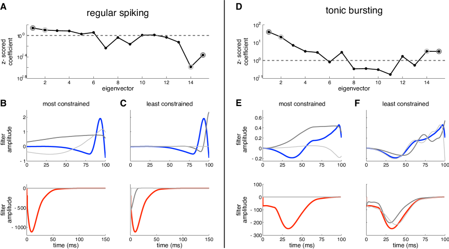
Figure 11: Sensitivity to changes in parameter values for a regular spiking (left) and tonic bursting (right) GLM. A: Fit coefficient of each eigenvector of Hessian matrix of likelihood, normalized by corresponding eigenvalue. Eigenvectors are in order of decreasing eigenvalues (not necessarily decreasing z-scored eigenvalues). B: Stimulus filter (top, blue) and spike history filter (bottom, red), along with two most constrained eigenvectors. These correspond to the largest (dark gray) and second largest (light gray) eigenvalues. Eigenvectors are scaled to size comparable with filters. C: Same as B, for least constrained eigenvectors. D-F: Same as A-D for tonic bursting neuron.

We wished to investigate how well constrained different features of our fit GLMs were. To do so, we calculated the eigendecomposition of the Hessian matrix of the likelihood function: $H=Q\Lambda Q^{-1}$. The Hessian matrix provides a local quadratic approximation to the likelihood function, with eigenvectors $q_{i}$ pointing along the principal axes and length of these axes proportional to $\frac{1}{\sqrt{\lambda_{i}}}$. Thus, larger magnitude eigenvalues indicate greater curvature (i.e., shorter axes) and better constrained directions, while smaller magnitude eigenvalues indicate lower curvature and more poorly constrained directions. Results of this analysis are shown in Figure 11 for both a regular spiking neuron (left) and tonic bursting neuron (right). For both neurons, the least constrained directions correspond to eigenvectors similar in shape to the best-fit filters or the absolute refractory period. As such, perturbations in these directions do not result in large changes in the behavior. Perturbations along eigenvectors corresponding to the most constrained directions, on the other hand, would result in significant changes to the filter shape. The difference in scale between Panel A and Panel D indicates that overall, parameters for the tonic bursting neuron are more constrained than those for the regular spiking neuron.

Doubly stochastic model with super-Poisson variability

In Figure 10, we used a negative binomial model to generate spike trains with greater-than-Poisson variability [38, 17]. The negative binomial distribution can be conceived as a doubly-stochastic model in which the rate of a Poisson process is modulated by an $iid$ gamma random variable on each trial. Following [17], we modeled responses with a stochastic gain variable $g$ with mean 1 and variance $\sigma_{g}^{2}$ that obeys a gamma distribution:

$$P(g|r,s)=\frac{1}{s^{r}\Gamma(r)}g^{r-1}\exp\left(-\frac{g}{s}\right),$$ (9)

where $s=\sigma_{g}^{2}$ denotes the scale parameter, $r=1/\sigma_{g}^{2}$ is the shape parameter, and $\Gamma(\cdot)$ represents the gamma function.

The spike count conditioned on $g$ and a stimulus $S$ for each trial then obeys a Poisson distribution:

$$P(y|g,S)=\frac{{\left(\Delta gf(S)\right)}^{y}}{y!}\exp\left(-\Delta gf(S)\right),$$ (10)

where $\Delta$ is the time bin size, $g$ is the gain, and $f(S)$ is the tuning curve that specifies the mean response to stimulus $S$. In the limit $\sigma_{g}^{2}=0$, the gain $g$ is deterministically equal to 1 and the spike count is Poisson with mean and variance equal to $\Delta f(S)$. For responses with $\sigma_{g}^{2}>0$, however, responses are overdispersed relative to the Poisson distribution and have mean $\Delta f(S)$ and variance $\Delta f(S)(1+\sigma_{g}^{2}\Delta f(S))$.

For the results shown in Figure 10, we simulated data from the negative binomial distribution with a single mean rate $f(S)$ (100 spikes/s) at three different gain variances $\sigma_{g}^{2}\in\{.0125,0.02,0.05\}$. Spike counts were drawn $iid$ across trials, with spike times distributed uniformly within each trial to generate spike trains suitable for GLM fitting. We used these spike trains to fit a GLM to the data associated with each value of $\sigma_{g}^{2}$, with an assumed constant input current for each trial.

References

- Ahrens et al., [2008] Ahrens, M. B., Linden, J. F., and Sahani, M. (2008). Nonlinearities and contextual influences in auditory cortical responses modeled with multilinear spectrotemporal methods. J Neurosci, 28(8):1929–1942.
- Babadi et al., [2010] Babadi, B., Casti, A., Xiao, Y., Kaplan, E., and Paninski, L. (2010). A generalized linear model of the impact of direct and indirect inputs to the lateral geniculate nucleus. Journal of Vision, 10(10):22.
- Berry and Meister, [1998] Berry, M. and Meister, M. (1998). Refractoriness and neural precision. Journal of Neuroscience, 18:2200–2211.
- Brette and Gerstner, [2005] Brette, R. and Gerstner, W. (2005). Adaptive exponential integrate-and-fire model as an effective description of neuronal activity. Journal of neurophysiology, 94(5):3637–3642.
- Calabrese et al., [2011] Calabrese, A., Schumacher, J. W., Schneider, D. M., Paninski, L., and Woolley, S. M. N. (2011). A generalized linear model for estimating spectrotemporal receptive fields from responses to natural sounds. PLoS One, 6(1):e16104.
- Cox and Isham, [1980] Cox, D. and Isham, V. (1980). Point Processes. Chapman & Hall/CRC Monographs on Statistics & Applied Probability. Taylor & Francis.
- Cui et al., [2013] Cui, Y., Liu, L. D., Khawaja, F. A., Pack, C. C., and Butts, D. A. (2013). Diverse suppressive influences in area mt and selectivity to complex motion features. The Journal of Neuroscience, 33(42):16715–16728.
- Fitzgerald et al., [2011] Fitzgerald, J. D., Rowekamp, R. J., Sincich, L. C., and Sharpee, T. O. (2011). Second order dimensionality reduction using minimum and maximum mutual information models. PLoS Comput Biol, 7(10):e1002249.
- FitzHugh, [1961] FitzHugh, R. (1961). Impulses and physiological states in theoretical models of nerve membrane. Biophysical journal, 1(6):445.
- Geisler and Goldberg, [1966] Geisler, C. D. and Goldberg, J. M. (1966). A Stochastic Model of the Repetitive Activity of Neurons. Biophysical Journal, 6(1):53–69.
- Gerhard et al., [2017] Gerhard, F., Deger, M., and Truccolo, W. (2017). On the stability and dynamics of stochastic spiking neuron models: Nonlinear hawkes process and point process glms. PLoS computational biology, 13(2):e1005390.
- Gerstner, [1995] Gerstner, W. (1995). Time structure of the activity in neural network models. Physical Review E, 51(1):738–758.
- Gerstner, [2001] Gerstner, W. (2001). A framework for spiking neuron models: The spike response model. In Moss, F. and Gielen, S., editors, The Handbook of Biological Physics, volume 4, pages 469–516.
- Gerstner et al., [2014] Gerstner, W., Kistler, W. M., Naud, R., and Paninski, L. (2014). Neuronal Dynamics: From Single Neurons to Networks and Models of Cognition. Cambridge University Press, New York, NY, USA.
- Gerstner and van Hemmen, [1992] Gerstner, W. and van Hemmen, J. (1992). Associative memory in a network of ‘spiking’ neurons. Network: Computation in Neural Systems, 3(2):139–164.
- Gerstner et al., [1996] Gerstner, W., van Hemmen, J. L., and Cowan, J. D. (1996). What matters in neuronal locking? Neural computation, 8:1653–1676.
- Goris et al., [2014] Goris, R. L. T., Movshon, J. A., and Simoncelli, E. P. (2014). Partitioning neuronal variability. Nat Neurosci, 17(6):858–865.
- Heitman et al., [2014] Heitman, A., Greschner, M., Field, G., Li, P., Ahn, D., Sher, A., Litke, A., and Chichilnisky, E. (2014). Representation and reconstruction of natural scenes in the primate retina. In Computational and Systems Neuroscience (CoSyNe) Abstracts, pages 134 – 135.
- Hocker and Park, [2017] Hocker, D. and Park, I. M. (2017). Multistep inference for generalized linear spiking models curbs runaway excitation. In 8th International IEEE EMBS Conference On Neural Engineering.
- Hodgkin, [1948] Hodgkin, A. (1948). The local electric changes associated with repetitive action in a non-medullated axon. The Journal of physiology, 107(2):165–181.
- Hodgkin and Huxley, [1952] Hodgkin, A. L. and Huxley, A. F. (1952). A quantitative description of membrane current and its application to conduction and excitation in nerve. J. Physiol., 117(4):500–544.
- Izhikevich, [2003] Izhikevich, E. M. (2003). Simple model of spiking neurons. IEEE Trans Neural Netw, 14(6):1569–1572.
- Izhikevich, [2004] Izhikevich, E. M. (2004). Which model to use for cortical spiking neurons? IEEE Trans Neural Netw, 15(5):1063–1070.
- Jolivet et al., [2003] Jolivet, R., Lewis, T., and Gerstner, W. (2003). The spike response model: a framework to predict neuronal spike trains. Springer Lecture notes in computer science, 2714:846–853.
- Jolivet et al., [2006] Jolivet, R., Rauch, A., Lüscher, H. R., and Gerstner, W. (2006). Predicting spike timing of neocortical pyramidal neurons by simple threshold models. Journal of Computational Neuroscience, 21(1):35–49.
- Keat et al., [2001] Keat, J., Reinagel, P., Reid, R., and Meister, M. (2001). Predicting every spike: a model for the responses of visual neurons. Neuron, 30:803–817.
- Latimer et al., [2014] Latimer, K. W., Chichilnisky, E. J., Rieke, F., and Pillow, J. W. (2014). Inferring synaptic conductances from spike trains with a biophysically inspired point process model. In Ghahramani, Z., Welling, M., Cortes, C., Lawrence, N., and Weinberger, K., editors, Advances in Neural Information Processing Systems 27, pages 954–962. Curran Associates, Inc.
- London and Häusser, [2005] London, M. and Häusser, M. (2005). Dendritic Computation. Annual Review of Neuroscience, 28(1):503–532.
- Mainen and Sejnowski, [1995] Mainen, Z. and Sejnowski, T. (1995). Reliability of spike timing in neocortical neurons. Science, 268:1503–1506.
- McFarland et al., [2013] McFarland, J. M., Cui, Y., and Butts, D. A. (2013). Inferring nonlinear neuronal computation based on physiologically plausible inputs. PLoS Comput Biol, 9(7):e1003143+.
- Mensi et al., [2012] Mensi, S., Naud, R., Pozzorini, C., Avermann, M., Petersen, C. C. H., and Gerstner, W. (2012). Parameter extraction and classification of three cortical neuron types reveals two distinct adaptation mechanisms. Journal of Neurophysiology, 107:1756–1775.
- Morris and Lecar, [1981] Morris, C. and Lecar, H. (1981). Voltage oscillations in the barnacle giant muscle fiber. Biophysical journal, 35(July):193–213.
- Nagumo et al., [1962] Nagumo, J., Arimoto, S., and Yoshizawa, S. (1962). An Active Pulse Transmission Line Simulating Nerve Axon. Proceedings of the IRE, 117(m V):2061–2070.
- Paninski, [2004] Paninski, L. (2004). Maximum likelihood estimation of cascade point-process neural encoding models. Network: Computation in Neural Systems, 15:243–262.
- Paninski et al., [2004] Paninski, L., Pillow, J. W., and Simoncelli, E. P. (2004). Maximum likelihood estimation of a stochastic integrate-and-fire neural model. Neural Computation, 16:2533–2561.
- Park et al., [2013] Park, I. M., Archer, E. W., Priebe, N., and Pillow, J. W. (2013). Spectral methods for neural characterization using generalized quadratic models. In Advances in Neural Information Processing Systems 26, pages 2454–2462.
- Perkel et al., [1967] Perkel, D. H., Gerstein, G. L., and Moore, G. P. (1967). Neuronal spike trains and stochastic point processes i. the single spike train. Biophysical Journal, 7(4):391–418.
- Pillow and Scott, [2012] Pillow, J. and Scott, J. (2012). Fully bayesian inference for neural models with negative-binomial spiking. In Bartlett, P., Pereira, F., Burges, C., Bottou, L., and Weinberger, K., editors, Advances in Neural Information Processing Systems 25, pages 1907–1915.
- Pillow et al., [2005] Pillow, J. W., Paninski, L., Uzzell, V. J., Simoncelli, E. P., and Chichilnisky, E. J. (2005). Prediction and decoding of retinal ganglion cell responses with a probabilistic spiking model. The Journal of Neuroscience, 25:11003–11013.
- Pillow et al., [2008] Pillow, J. W., Shlens, J., Paninski, L., Sher, A., Litke, A. M., and Chichilnisky, E. J. Simoncelli, E. P. (2008). Spatio-temporal correlations and visual signaling in a complete neuronal population. Nature, 454:995–999.
- Pozzorini et al., [2013] Pozzorini, C., Naud, R., Mensi, S., and Gerstner, W. (2013). Temporal whitening by power-law adaptation in neocortical neurons. Nature Neuroscience, 16(7):942–948.
- Rabinowitz et al., [2015] Rabinowitz, N. C., Goris, R. L., Cohen, M., and Simoncelli, E. (2015). Attention stabilizes the shared gain of v4 populations. eLife.
- Rajan et al., [2013] Rajan, K., Marre, O., and Tkačik, G. (2013). Learning quadratic receptive fields from neural responses to natural stimuli. Neural Computation, 25(7):1661–1692.
- Schneidman et al., [1998] Schneidman, E., Freedman, B., and Segev, I. (1998). Ion channel stochasticity may be critical in determining the reliability and precision of spike timing. Neural computation, 10(7):1679–703.
- Shadlen and Newsome, [1998] Shadlen, M. and Newsome, W. (1998). The variable discharge of cortical neurons: implications for connectivity, computation, and information coding. Journal of Neuroscience, 18:3870–3896.
- Tolhurst et al., [1983] Tolhurst, D. J., Movshon, J. A., and Dean, A. F. (1983). The statistical reliability of signals in single neurons in cat and monkey visual cortex. Vision Res, 23(8):775–785.
- Tomko and Crapper, [1974] Tomko, G. J. and Crapper, D. R. (1974). Neuronal variability: non-stationary responses to identical visual stimuli. Brain research, 79(3):405–418.
- Truccolo et al., [2005] Truccolo, W., Eden, U. T., Fellows, M. R., Donoghue, J. P., and Brown, E. N. (2005). A point process framework for relating neural spiking activity to spiking history, neural ensemble and extrinsic covariate effects. J. Neurophysiol, 93(2):1074–1089.
- Uzzell, [2004] Uzzell, V. J. (2004). Precision of Spike Trains in Primate Retinal Ganglion Cells. Journal of Neurophysiology, 92(2):780–789.
- Weber et al., [2012] Weber, F., Machens, C. K., and Borst, A. (2012). Disentangling the functional consequences of the connectivity between optic-flow processing neurons. Nature neuroscience, 15(3):441–448.
- Weiss, [1966] Weiss, T. F. (1966). A model of the peripheral auditory system. Kybernetik, 3(4):153–175.
- Williamson et al., [2015] Williamson, R. S., Sahani, M., and Pillow, J. W. (2015). The equivalence of information-theoretic and likelihood-based methods for neural dimensionality reduction. PLoS Comput Biol, 11(4):e1004141.
- Zhao and Iyengar, [2010] Zhao, M. and Iyengar, S. (2010). Nonconvergence in logistic and poisson models for neural spiking. Neural Computation, 22(5):1231–1244. PMID: 20100077.