Automatic moth detection from trap images for pest management

Abstract

Monitoring the number of insect pests is a crucial component in pheromone-based pest management systems. In this paper, we propose an automatic detection pipeline based on deep learning for identifying and counting pests in images taken inside field traps. Applied to a commercial codling moth dataset, our method shows promising performance both qualitatively and quantitatively. Compared to previous attempts at pest detection, our approach uses no pest-specific engineering which enables it to adapt to other species and environments with minimal human effort. It is amenable to implementation on parallel hardware and therefore capable of deployment in settings where real-time performance is required.

1 Introduction

Monitoring is a crucial component in pheromone-based pest control [1, 2] systems. In widely used trap-based pest monitoring, captured digital images are analysed by human experts for recognizing and counting pests. Manual counting is labour intensive, slow, expensive, and sometimes error-prone, which precludes reaching real-time performance and cost targets. Our goal is to apply state-of-the-art deep learning techniques to pest detection and counting, effectively removing the human from the loop to achieve a completely automated, real-time pest monitoring system.

Plenty of previous work has considered insect classification. The past literature can be grouped along several dimensions, including image acquisition settings, features, and classification algorithms. In terms of image sources, many previous methods have considered insect specimens [3, 4, 5, 6, 7, 8]. Specimens are usually well preserved and imaged in an ideal lab environment. Thus specimen images are consistent and captured at high resolution. In a less ideal but more practical scenario, some other works attempt to classify insects collected in the wild, but imaged under laboratory conditions [9, 10, 11, 12, 13, 14, 15]. In this case, image quality is usually worse than the specimen case, but researchers still typically have a chance to adjust settings to control image quality, such as imaging all of the insects under a standard orientation or lighting.

From an algorithmic perspective, various types of features have been used for insect classification, including wing structures [3, 4, 5, 6, 7], colour histogram features [16, 17], morphometric measurements [18, 19, 7, 8], local image features [16, 17, 20, 21, 22, 23], and global image features [24]. Different classifiers were also used on top of these various feature extraction methods, including support vector machines (SVM) [20, 8, 11], artificial neural networks (ANN) [8, 17, 18], k-nearest neighbours (KNN) [24, 21], and ensemble methods [9, 10, 21]. In general, however, these proposed methods were not tested under real application scenarios, for example, images from real traps deployed for pest monitoring.

Object detection involves also localizing objects in addition to classification. A few attempts have been made with respect to insect detection. One option is to perform a “sliding window” approach, where a classifier scans over patches at different locations of the image. This technique was applied for inspection of bulk wheat samples [25], where local patches from the original image were represented by engineered features and classified by discriminant analysis. Another work on bulk grain inspection [26] employed different customized rule-based algorithms to detect different objects, respectively. The other way of performing detection is to first propose initial detection candidates by performing image segmentations. These candidates are then represented by engineered features and classified [27, 28]. All of these insect detection methods are heavily engineered and work only on specific species under specific environments, and are not likely to be directly effective in the pest monitoring setting.

There are two main challenges in detecting pests from trap images. The first challenge is low image quality, due to constraints such as the cost of the imaging sensor, power consumption, and the speed by which images can be transmitted. This makes most of the previous work impractical, that is, those based on high image quality and fine structures. The second challenge comes from inconsistencies which are driven by many factors, including illumination, movement of the trap, movement of the moth, camera out of focus, appearance of other objects (such as leaves), decay or damage to the insect, appearance of non-pest (benign) insects, etc. These make it very hard to design rule-based systems. Therefore, an ideal detection method should be capable and flexible enough to adapt to different varying factors with a minimal amount of additional manual effort other than manually labelled data from a daily pest monitoring program.

Apart from the insect classification/detection community, general visual object category recognition and detection has been a mainstay of computer vision for a long time. Various methods and datasets [29, 30] have been proposed in the last several decades to push this area forward. Recently, convolutional neural networks (ConvNets) [31, 32] and their variants have emerged as the most effective method for object recognition and detection, by achieving state-of-the-art performance on many well recognized datasets [33, 34, 35], and winning different object recognition challenges [36, 32, 37].

Inspired by this line of research, we adopt the popular sliding window detection pipeline with convolutional neural networks as the image classifier. First, raw images are preprocessed with colour correction. Then, trained ConvNets are applied to densely sampled image patches to predict each patch’s likelihood of containing pests. Patches are then filtered by non-maximum suppression, after which only those with probabilities higher than their neighbours are preserved. Finally, the remaining patches are thresholded. Patches whose probability meet the threshold are considered as proposed detections.

This paper makes two main contributions. First, we develop a ConvNet-based pest detection method, that is accurate, fast, easily extendable to other pest species, and requires minimal pre-processing of data. Second, we propose an evaluation metric for pest detection borrowing ideas from the pedestrian detection literature.

2 Data collection

In this section, we describe the collection, curation, and preprocessing of images. Details of detection performed on processed images are provided in Section 3.

2.1 Data acquisition

RGB colour images are captured by pheromone traps installed at multiple locations by a commercial provider of pheromone-based pest control solutions, whose name is withheld by request. The trap contains a pheromone lure, an adhesive liner, a digital camera and a radio transmitter. The pheromone attracts the pest of interest into the trap where they become stuck to the adhesive surface. The digital images are stored in JPEG format at 640$\times$480 resolution, and transmitted to a remote server at fixed time point daily. Codling moths are identified and labelled with bounding boxes by technicians trained in entomology. Only one image from each temporal sequence is labelled and used in this study, so labelled images do not have temporal correlation with each other. As a result, all of the labelled moths are unique. Figure 1(a) shows a trap image with all the codling moth labelled with blue bounding boxes. Figure 1(b) shows an image containing no moths but cluttered with other types of insects. High resolution individual image patches are shown later in Figure 11, with their characteristics analysed in Section 5.3.

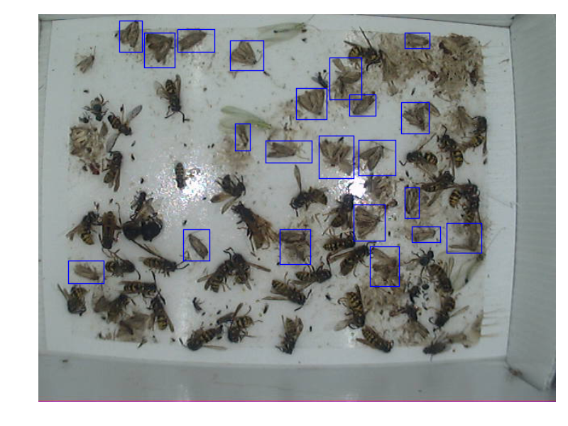
(a) Trap containing moths. Blue rectangles indicate codling moths labelled by technicians.

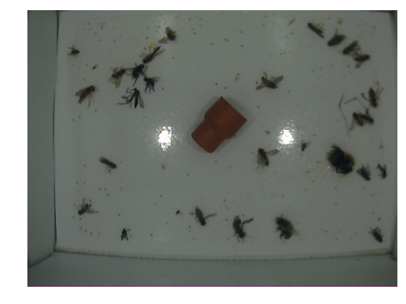
(b) Trap containing no moths. The large object in the centre is a pheromone lure.

Figure 1: Examples of images captured within the pheromone traps. Best viewed in colour.

2.2 Dataset construction

The set of collected images is split randomly into 3 sets: the training set, the validation set and the test set. After splitting, the statistics of each set is roughly the same as the entire dataset, including the ratio between the number of images with or without moths, and number of moths per image. Table 1 provides specific statistics on the entire dataset and the three splits subsequently constructed.

Dataset	Total #	# images with moth	# images without moth	# moths	avg. # moths per image
Total	177	133	44	4447	25.1
Training	110	83	27	2724	24.8
Validation	27	20	7	690	25.6
Test	40	30	10	1033	25.8

Table 1: Statistics of constructed datasets.

2.3 Preprocessing

Trap images were collected in real production environments, which leads to different imaging conditions at different points in time. This is most apparent in illumination, which can be seen in Figure 2(a). To eliminate the potential negative effects of illumination variability on detection performance, we perform colour correction using one variant [38] of the “grey-world” method. This algorithm assumes that the average value of red (R), green (G) and blue (B) channels should equal to each other. Specifically, for each image, we set the gain of the R and B channels as follows:

$$G_{red}=\mu_{red}/\mu_{green},~{}G_{blue}=\mu_{blue}/\mu_{green}$$ (1)

where $\mu_{red}$, $\mu_{green}$ and $\mu_{blue}$ are the original average intensities of the red, green and blue channels, respectively. $G_{red}$ and $G_{blue}$ are multiplicative gains applied to the pixel intensity values of the red and blue channels, respectively. Figure 2(b) shows images processed by the grey-world algorithm. We see that the images are white-balanced to have similar illumination, but still maintain rich colour information which can be a useful cue for detection downstream. In this paper, all images are white-balanced prior to detection.

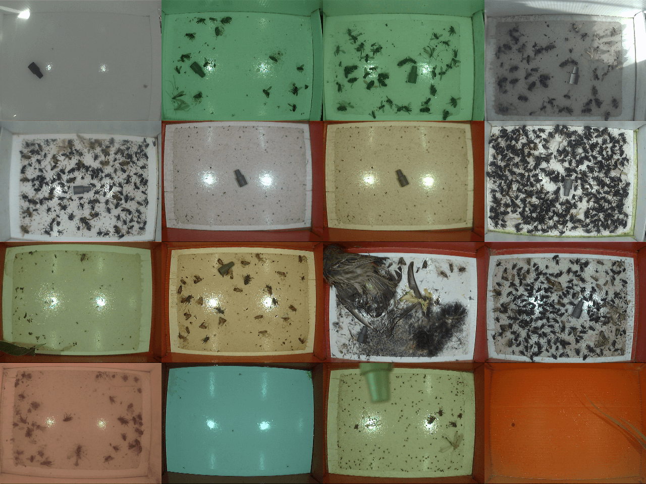
(a) Original images

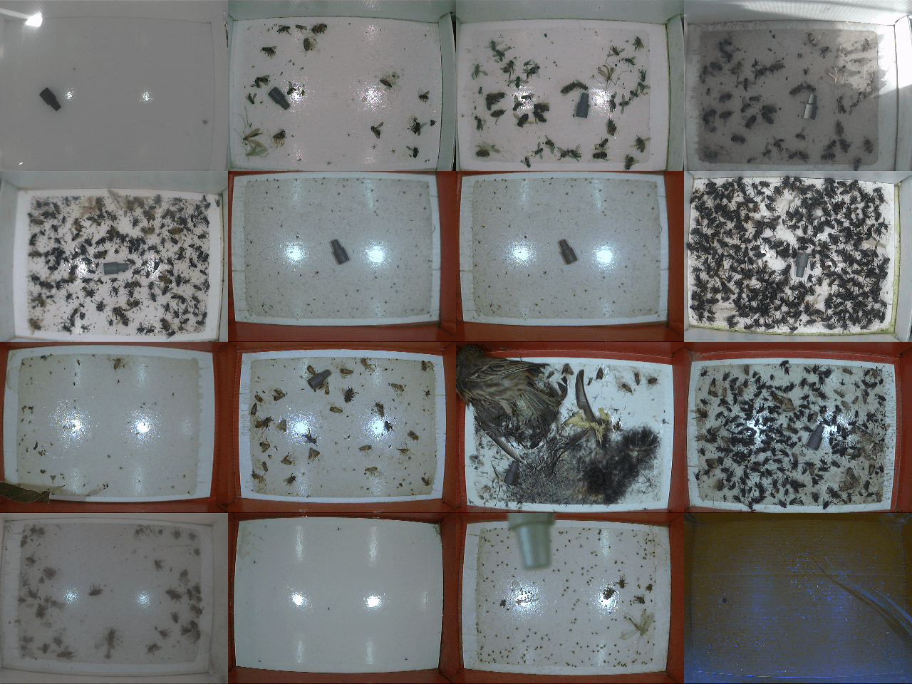
(b) Images processed by the “grey world” algorithm [38].

Figure 2: Illustration of grey world colour correction. Best viewed in colour.

3 Detection pipeline

The automatic detection pipeline involves several steps, as shown in Figure 3. We take a sliding window approach, where a trained image classifier is applied to local windows at different locations of the entire image. The classifier’s output is a single scalar $p\in[0,1]$, which represents the probability that a particular patch contains a codling moth. These patches are regularly and densely arranged over the image, and thus largely overlapping. Therefore, we perform non-maximum suppression (NMS) to retain only the windows whose respective probability is locally maximal. The remaining boxes are then thresholded, such that only patches over a certain probability are kept. The location of these patches with their respective probabilities (confidence scores) are the final outputs of the detection pipeline. We now discuss each of these stages in more detail.

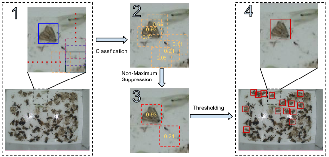
Figure 3: Illustration of the detection pipeline. Best viewed in colour.

3.1 Convolutional neural networks

In a sliding window approach, the detection problem breaks down into classifying each local patch, which is performed by the image classifier $C$, a mapping from the image $I$ to a probability $p$: $C:I\mapsto p$. We adopt convolutional neural network [31] (ConvNet) as our image classifier, as it is the most popular and best performing classifier for image recognition in both large scale [32, 37] and small scale [39, 40] problems. It is also very fast to deploy, and amenable to parallel hardware. Specifically, we used a network structure similar to Lenet5 [31]. As shown in Figure 4, our network contains 2 convolutional layers, 2 max-pooling layers, and 2 fully connected layers (described below). Before applying the ConvNet, each dimension of the input patch is normalized to have zero mean and unit variance.

3.1.1 Convolutional layers

A convolutional layer applies a linear filterbank and element-wise nonlinearity to its input “feature maps”, transforming them to a different set of feature maps. By applying convolutional layers several times, we can extract increasingly high-level feature representations of the input, at the same time preserving their spatial relationship. At the first layer, the input feature maps are simply the channels of the input. At subsequent layers, these represent more abstract transformations of the image. A convolutional layer is a special case of a fully connected layer, introduced in Subsection 3.1.3, where only local connections are have non-zero values, and weights are tied at all locations. Local connectivity is implemented efficiently by applying convolution:

$$\boldsymbol{h}^{l}_{k}=\varphi\left(\sum_{m}\boldsymbol{W}^{l}_{m,k}\boldsymbol{h}^{l-1}_{m}+\boldsymbol{b}^{l}_{k}\right)~{},$$ (2)

where $l$ is the layer index; $m$ is the index of input feature maps; $k$ is the index of output feature maps; input $\boldsymbol{h}^{l-1}_{m}$ is the $m$th feature map at layer $l-1$; output $\boldsymbol{h}^{l}_{k}$ the $k$th feature map at layer $l$; $\boldsymbol{W}$ is the convolutional weight tensor; $\boldsymbol{b}$ is the bias term; and we choose the element-wise nonlinearity $\varphi(\cdot)$ to be the rectified linear unit (RELU) [41] function.

3.1.2 Max-pooling layers

Each convolutional layer is followed by a max-pooling layer. This layer applies local pooling operations to its input feature maps, by only preserving the maximum value within a local receptive field and discarding all other values. It is similar to a convolutional layer in the sense that both operate locally. Applying max-pooling layers has 2 major benefits: 1) reducing the number of free parameters, and 2) introducing a small amount of translational invariance into the network.

3.1.3 Fully connected layers

The last two layers in our ConvNet are fully connected. These are the kind of layers found in standard feed-forward neural networks. The first fully connected layer flattens (vectorizes) all of the feature maps after the last max-pooling layer, treating this one-dimensional vector as a feature representation of the whole image. The second fully connected layer is parameterized like a linear classifier. Mathematically, the fully connected layer can be written as:

$$\boldsymbol{h}^{l}=\varphi(\boldsymbol{W}^{l}\boldsymbol{h}^{l-1}+\boldsymbol{b}^{l}),$$ (3)

where $l$ is the layer index; input $\boldsymbol{h}^{l-1}$ is the vector representation at layer $l-1$; $\boldsymbol{h}^{l}$ is the output of layer $l$; $\boldsymbol{W}$ is the weight matrix; $\boldsymbol{b}$ is the bias vector; and $\varphi(\cdot)$ is an element-wise nonlinear function: we choose RELUs for the fully connected hidden layer and a softmax for the output layer.

For a more detailed explanation of convolutional neural networks, we refer the reader to [31, 32, 42].

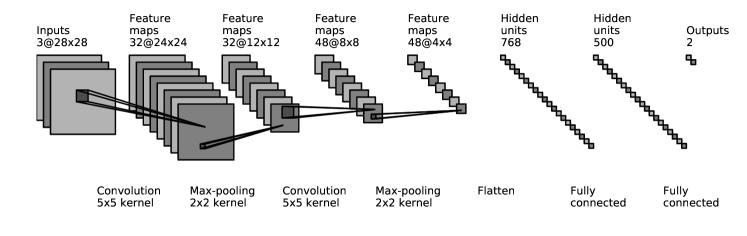
Figure 4: The convolutional neural network architecture used in our experiments.

3.2 Non-maximum suppression

After applying the ConvNet in a sliding window fashion, we obtain probabilities associated with each densely sampled patch. If we simply applied thresholding at this point, we would get many overlapping detections. This problem is commonly solved using non-maximum suppression (NMS) which aims to retain only patches with locally maximal probability. We adopted a strategy similar to [43]. Specifically, we first sort all the detections according to their probability. Then, from high to low probability, we look at each detection and remove other bounding boxes that overlap at least 10% with the current detection. After this greedy process, we generate final detection outputs as shown in Figure 3 and later in Section 5.1.

4 Experiments and evaluation

We next introduce how we performed the experiments and the evaluation protocol.

4.1 Classifier training

The classifier is trained on generated patches of different sizes, detailed in Section 4.2. Minibatch stochastic gradient descent (SGD) with momentum [44] was used to train the ConvNet. The gradient is estimated with the well known back-propagation algorithm [45]. We used a fixed learning rate of 0.002, a fixed minibatch size of 256, and a fixed momentum coefficient of 0.9. The validation set is used for monitoring the training process and selecting hyper-parameters. We report performance using a classifier whose parameters are chosen according to the best observed validation set accuracy. The filters and fully-connected weight matrices of the ConvNets are initialized with values selected from a uniform random distribution on an interval that is a function of the number of pre-synaptic and post-synaptic units (see [46] for more detail).

4.2 Training data extraction

In the sliding window classification pipeline, the classifier takes a local window as its input. Therefore we need to extract small local patches from the original high-resolution to train the classifier. This is performed in a memory-efficient manner, using pointer arithmetic to create “views” to the data as opposed to storing all patches in memory.

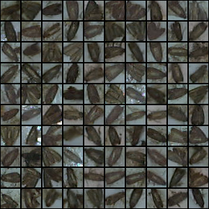
(a) Patches containing a moth

(b) Initial negative patches

(c) Negative patches after bootstrapping

Figure 5: Some examples of patches used for training the classifier.

4.2.1 Positive patches

Here, “positive patch” refers to patches derived from manually labelled bounding boxes, where each one represents a codling moth. As the the ConvNet processes square inputs, we ignored the original aspect ratio of the manually labelled bounding boxes, and took the square region having the same centre as the original rectangular bounding box. Figure 5(a) shows positive patches extracted from the training set.

4.2.2 Negative patches

It would be difficult to cover all the kinds of false positives that may arise by simply sampling the regions not covered by the labelled bounding boxes. This is because the area of regions not containing moths is much larger than the area covered by the bounding boxes. On images which are not very cluttered, most of the “negative” area is uninteresting (e.g. trap liner).

Thus, to obtain negative training examples, we intentionally take “hard” patches, meaning those which contain texture. Specifically, we apply the Canny edge detector [47] to find patches in “negative images”, i.e., those that do not contain any moths. We set the threshold such that the number of negative patches roughly matches the number of labelled moths. Figure 5(b) shows a random sample of negative patches.

4.2.3 Bootstrapping

After the initial set of negative patches are extracted, we use a bootstrapping approach to find useful negative training patches that can make the classifier more discriminative. In the first round of training, the initially generated patches are used to train the classifier. At test time, the false positive patches from the training set are collected, and we isolate the 6000 negative patches with highest probability assigned by the classifier. These are merged with the initially generated patches to form a new dataset for a second stage of training. One could potentially use more rounds of bootstrapping to collect more informative negative patches, but we found that including more than two training stages does not improve performance. Figure 5(c) shows randomly sampled patches collected in the test phase after one stage of training. For the validation set, the number of patches we collect is proportional to the number of images in the validation set.

4.3 Data augmentation

For machine learning-based methods, it is usually the case that the larger the dataset, the better the generalization performance. In our case, the amount of training data, which is represented by the number of training patches, is much smaller than standard small-scale image classification datasets [40, 48] frequently used by the deep learning community, which have on the order of 50,000 training examples. Therefore, we performed data augmentation to increase the number of images for training, and also incorporate invariance to basic geometric transformations into the classifier. Based on the “top-view” nature of the trap images, a certain patch will not change its class label when it is slightly translated, flipped, or rotated. Therefore, we apply these simple geometric transformations to the original patches to increase the number of training examples. For each patch, we create 8 translated copies by shifting $\pm$ 3 pixels horizontally, vertically, and diagonally. We also create versions which are flipped across the horizontal- and vertical-axes. Finally, we create 4 rotated copies by rotating the original by 0, 90, 180 and 270 degrees. This produces 72 augmented patches from one original. Figure 6 shows the augmented versions which are produced from a single example.

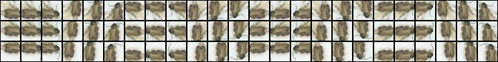
Figure 6: Data augmentation from a single example by translating, rotating, and flipping. Note that all copies retain the same (positive) label.

4.4 Detection

At the detection stage, we need to set the stride, which means the distance between adjacent sliding windows. A smaller stride means denser patch coverage, which lead to better localization of the moths, but also requires more computation. As a trade-off, we set the stride to be $\frac{1}{4}$ the size of a patch.

4.5 Evaluation protocol

Pest detection is still a relatively “niche” area of computer vision and therefore there is no standard evaluation protocol defined. We decided to adopt a protocol inspired by standardization within the pedestrian detection community. A complete overview is provided in [49] which we summarize below.

4.5.1 Matching detections with ground truth

We evaluate detection performance based on the statistics of misdetections, correct detections and false positives. Here, a misdetection refers to a manually labelled region which is missed by the algorithm, and a false positive refers a bounding box proposed by the algorithm which does not correspond to any manually labelled region. To determine if a bounding box proposed by the detector is a correct detection or a misdetection, we determine its correspondence to a a manually labelled bounding box by calculating the intersection-over-minimum (IOMin) heuristic:

$$A(BB_{dt},BB_{gt})=\frac{area(BB_{dt}\cap BB_{gt})}{min(area(BB_{dt}),area(BB_{gt}))}~{},$$ (4)

where $BB_{dt}$ represents a bounding box proposed by the algorithm (a detection) and $BB_{gt}$ represents a ground truth bounding box. We consider a specific ground truth bounding box, $BB_{gt}^{i}$, to be correctly detected when there exists a detection, $BB_{dt}^{j}$, such that $A(BB_{dt}^{j},BB_{gt}^{i})>0.5$. Otherwise, that ground truth bounding box is considered to be a misdetection. When multiple $BB_{dt}$’s satisfy the condition, the one with the highest probability under the classifier is chosen. After this is performed for all of the $BB_{gt}$, the remaining unmatched $BB_{dt}$ are considered to be false positives.

Our evaluation metric differs from that used by the pedestrian detection in that we use IOMin in place of the more popular Jaccard index, also called intersection-over-union (IOU). This is because of potential shape mismatches between the ground truth and detections. The ground truth bounding boxes are all rectangles, but our classifier outputs probabilities over square patches. In the case when the ground truth rectangle is nearly square, the IOU works well. In the case where the ground truth rectangle is tall or wide, however, the IOU tends to be small no matter how good the detection is. On the contrary, the IOMin heuristic performs well for both cases.

4.5.2 Object level evaluation

Based on the statistics of correct detections (also known as true positives), misdetections (also known as false negatives) and false positives, we could evaluate the performance at two levels: (1) object level, where the focus is on the performance of detecting individual moths; and (2) image level, where the focus is on determining whether or not an image contains any moths.

At the object level, we use five threshold-dependent measures: miss rate, false positives per image (FPPI), precision, recall, and $F_{\beta}$ score:

miss rate $$=\frac{\text{number of misdetections}}{\text{total number of moths}}$$ (5)

FPPI $$=\frac{\text{number of false positives}}{\text{total number of images}}$$ (6)

precision $$=\frac{\text{number of correct detections}}{\text{total number of detections}}$$ (7)

recall $$=\frac{\text{number of correct detections}}{\text{total number of moths}}$$ (8)

$$F_{\beta} =(1+\beta^{2})\frac{\text{precision}\cdot\text{recall}}{\beta^{2}\cdot\text{precision}+\text{recall}}$$ (9)

All quantities, with the exception of FPPI, are calculated by including correspondences across the entire dataset, and do not represent averages over individual images.

There are two pairs of metrics that measure the trade-off between reducing misdetections and reducing false positives: miss rate vs. FPPI, and precision vs. recall. Miss rate vs. FPPI is a common performance measure in the pedestrian detection community [49]. It gives an estimate of the system accuracy under certain tolerances specified by the number of false positives. Similarly, a precision vs. recall plot shows the trade-off between increasing the accuracy of detection and reducing misdetections.

The $F_{\beta}$ score is simply a measure which aims to weight the importance of precision and recall at a single operating point along the precision-recall curve. The larger it is, the better the performance. The parameter $\beta$ adjusts the importance between precision and recall. In this paper, we consider detecting all moths more important than reducing false positives, and therefore we more heavily weight recall, setting $\beta=2$ for all reported results.

Of course, there will be one $F_{\beta}$ score for each operating point (threshold) of the system. To summarize the information conveyed by the miss rate vs. FPPI and precision vs. recall plots by a single value, we employ two scalar performance measures: (1) log-average miss rate when FPPI is in the range [1, 10], and (2) area under the precision-recall curve (AUC).

4.5.3 Image level evaluation

Image level performance evaluation is considered for the scenario of semi-automatic detection, where the algorithm proposes images for a technician to inspect and safely ignores images that do not contain any moths. In this setting, the algorithm simply needs to make a proposal of “moths” or “no moths” per image regardless of how many moths it believes are present. Here we will call a “true moth” image an image that contains at least one moth, and a “no moth” image an image that contains no moths. Similar to Object Level Evaluation, there are five threshold-dependent measures: sensitivity (synonymous with recall), specificity, precision, and $F_{\beta}$ score:

$$\text{sensitivity}=\text{recall} =\frac{\text{number of correctly identified true moth images}}{\text{total number of true moth images}}$$ (10)

specificity $$=\frac{\text{number of correctly identified no moth images}}{\text{total number of no moth images}}$$ (11)

precision $$=\frac{\text{number of correctly identified true moth images}}{\text{total number of moth image proposals}}$$ (12)

where $F_{\beta}$ is defined in Eq. 9. Similar to object level evaluation, there are also two pairs of trade-offs: sensitivity vs. specificity, and precision vs. recall. For scalar performance measures, we calculate the AUC for both of these curves.

5 Results

In this section, we first give some visual (qualitative) results and then describe the results of the performance evaluation introduced in Section 4.

5.1 Qualitative

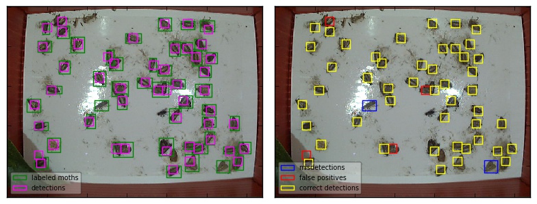
(a) ConvNet with input size $21\times 21$.

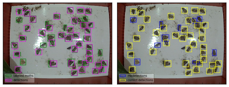
(b) ConvNet with input size $35\times 35$.

Figure 7: Visual example of detection results. Panel (a) shows the best-performing classifier at the object level. Panel (b) shows the best-performing classifier at the image level. Best viewed in colour.

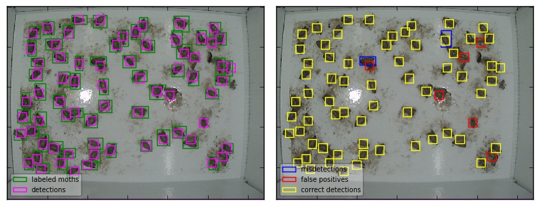
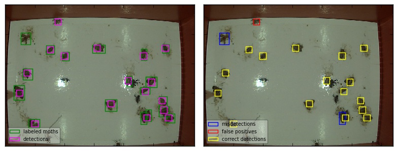
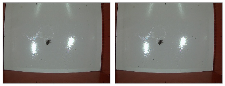
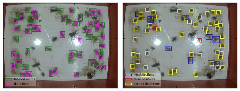
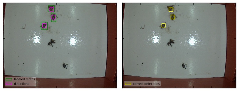
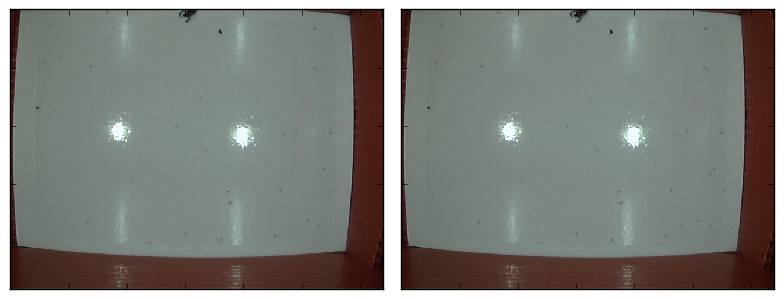
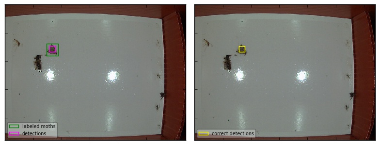
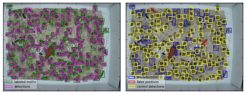
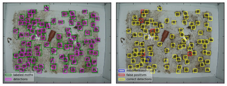
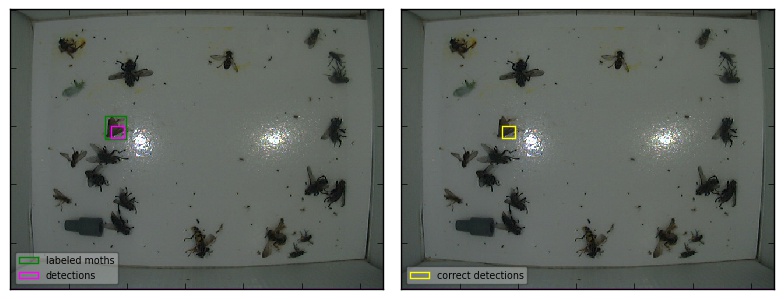
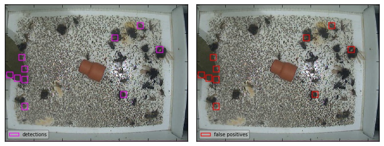
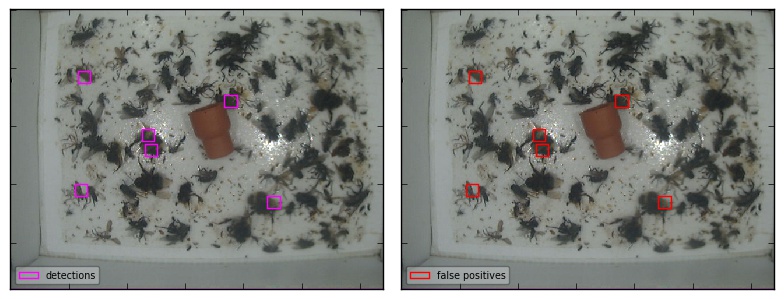
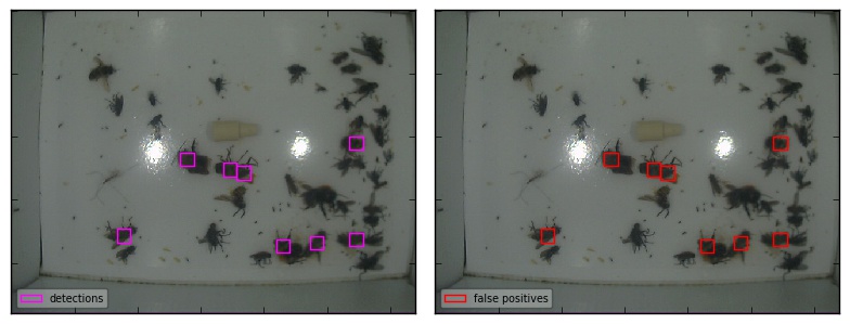
Figure 9: More examples of ConvNet with input size $21\times 21$. Best viewed in colour.

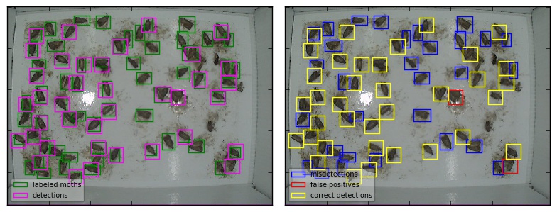
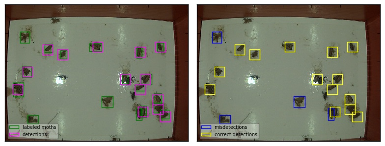
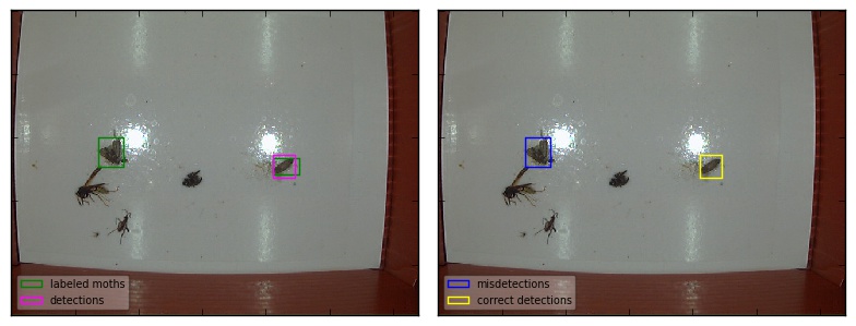
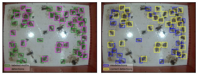
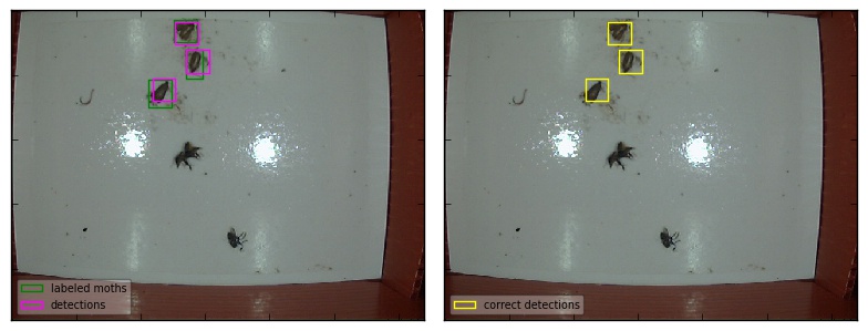
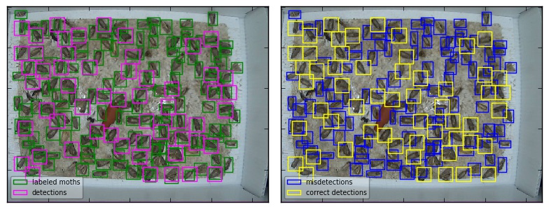
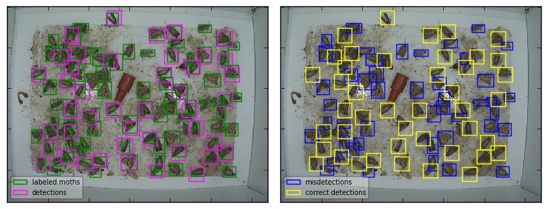
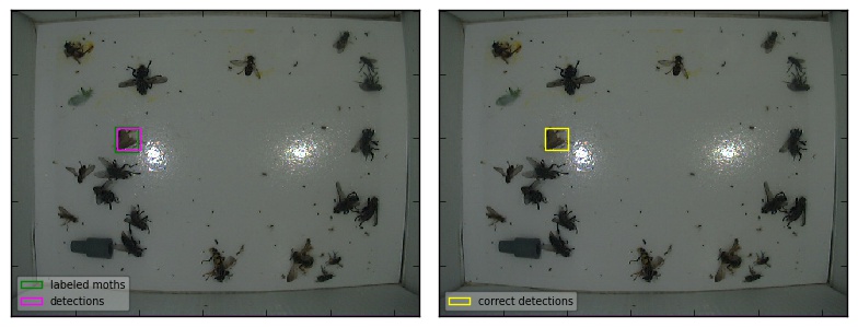
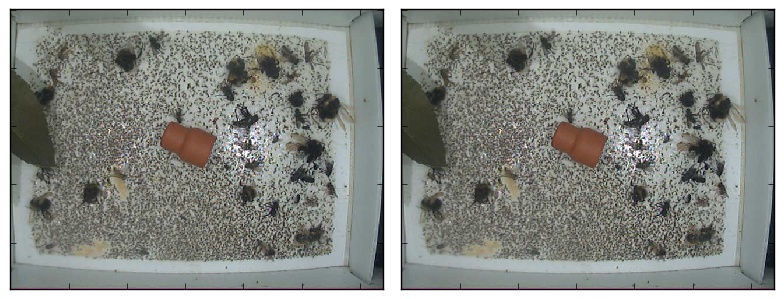
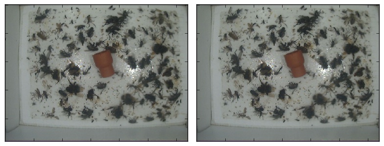
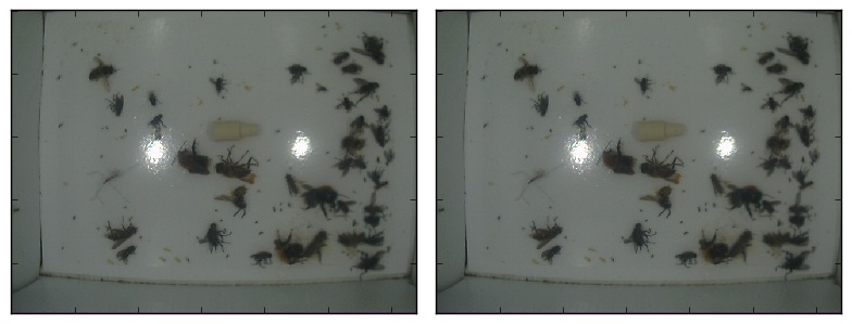
Figure 10: More examples of ConvNet with input size $35\times 35$. Best viewed in colour.

Figure 7 shows an example of our detector in operation. In both panels, the image on the left shows manually annotated bounding boxes in green and the proposals of our detector in magenta. The image on the right shows the results of matching annotations with proposals. Misdetections, false positives and correct detections are shown in blue, red, and yellow boxes respectively. In Figure 7(a) and 7(b), the thresholds are set to maximize the F2-score at the object level and the image level respectively. Figures 9 and 10 show more examples of detection results on full-sized images.

5.2 Quantitative

Method	Patch size	Object level		Image Level
		prec-rec AUC	log-avg miss rate	prec-rec AUC	sens-spec AUC
ConvNet	21$\times$21	0.931	0.099	0.972	0.888
	28$\times$28	0.879	0.135	0.987	0.913
	35$\times$35	0.824	0.200	0.993	0.932
	42$\times$42	0.713	0.315	0.989	0.925
	49$\times$49	0.612	0.404	0.988	0.922
LogReg	21$\times$21	0.555	0.756	0.782	0.682
	28$\times$28	0.621	0.586	0.765	0.665
	35$\times$35	0.658	0.491	0.815	0.713
	42$\times$42	0.582	0.496	0.852	0.755
	49$\times$49	0.499	0.545	0.808	0.713

Table 2: Performance of convolutional neural networks compared to logistic regression with different input sizes. ​Bold values represent the best performance per-method and per-metric.

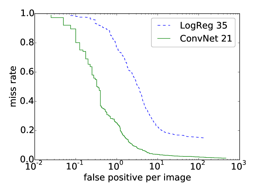
(a) miss rate-FPPI at object level

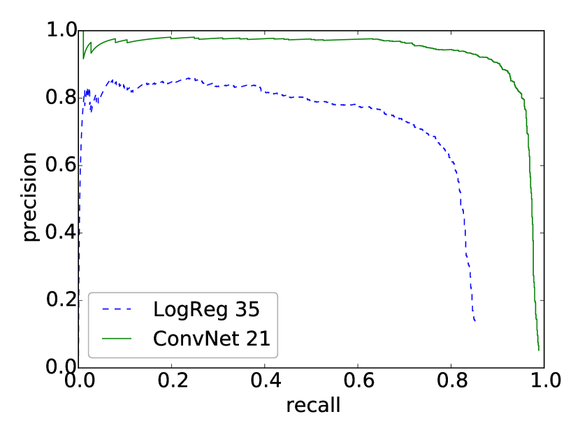
(b) precision-recall at object level

(c) $F_{2}$ score-threshold at object level

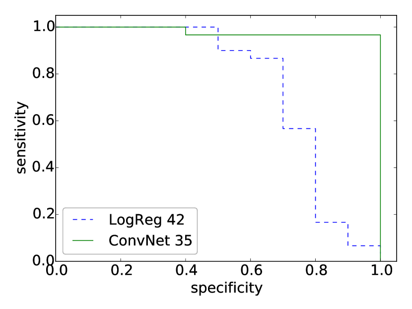
(d) sensitivity-specificity at image level

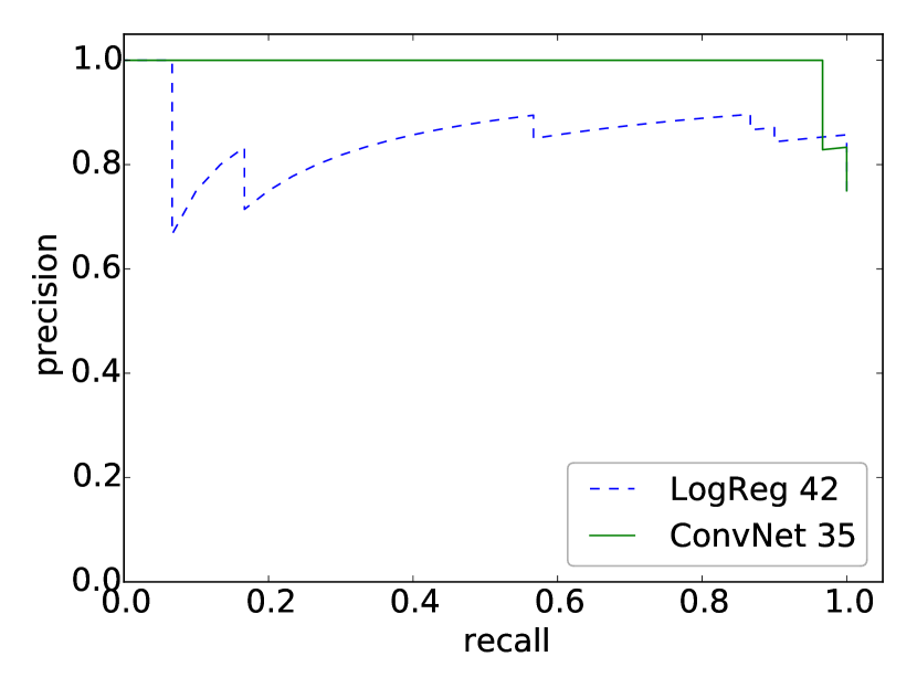
(e) precision-recall at image level

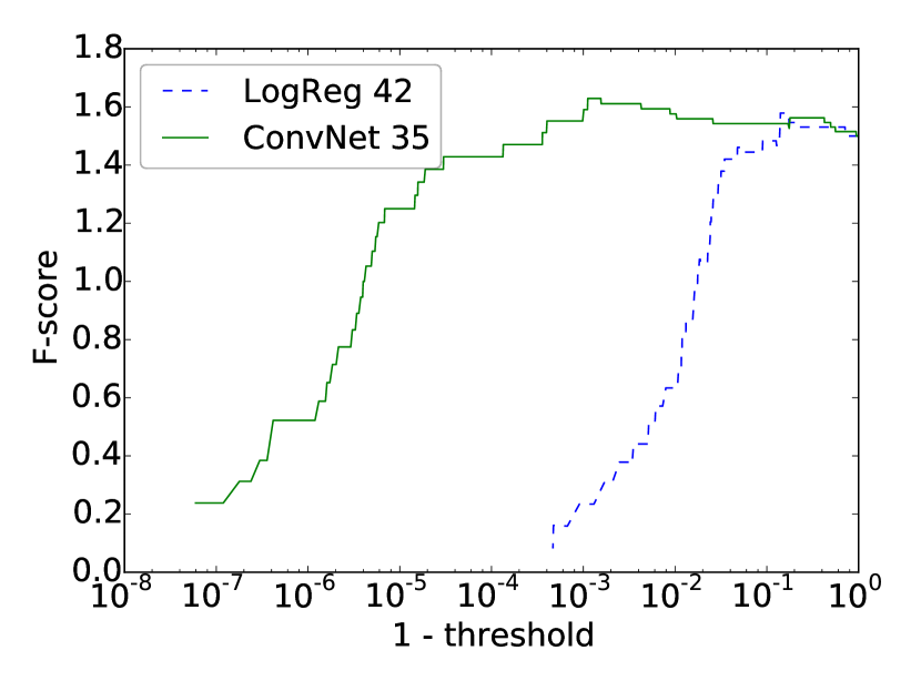
(f) $F_{2}$ score-threshold at image level

Figure 8: Comparison between the best performing ConvNets and logistic regression models at both the object and image level.

Method	Object Level		Image Level
	prec-rec AUC	log-avg miss rate	prec-rec AUC	sens-spec AUC
ConvNet + Trans&Rot Aug	0.931	0.099	0.972	0.888
ConvNet + Rot Aug	0.916	0.140	0.981	0.900
ConvNet + Trans Aug	0.879	0.204	0.979	0.892
ConvNet + No Aug	0.825	0.334	0.920	0.797

Table 3: Effectiveness of data augmentation.

Remaining	Object Level		Image Level
percentage	prec-rec AUC	log-avg miss rate	prec-rec AUC	sens-spec AUC
100%	0.931	0.099	0.972	0.888
80%	0.923	0.121	0.984	0.905
60%	0.906	0.155	0.979	0.883
40%	0.886	0.184	0.969	0.882
20%	0.895	0.233	0.941	0.835

Table 4: Influence of missing training data.

We chose logistic regression as a baseline for comparison to ConvNets. We tested both logistic regression and ConvNets at five different input sizes: 21$\times$21, 28$\times$28, 35$\times$35, 42$\times$42, and 49$\times$49. The results are shown in Table 2. The ConvNet with input size 21$\times$21 achieved the best performance at the object level and the ConvNet with input size 35$\times$35 had the best performance at the image level. Accordingly, Figure 8 shows different performance curves comparing the best performing ConvNet and logistic regression, both at the object and image level. Apparent from Figure 8 (d) and (e), the ConvNet achieved nearly perfect results at the image level. For the precision-recall curve, one usually expects precision to decrease as recall increases. Here, in Figure 8 (b) and (e), precision sometimes increases as the recall increases. This is because when the threshold is decreasing, it is possible that the newly included detections are all true detections, which results in an increase in both precision and recall.

To understand the effect of data augmentation (Section 4.3) on detector performance, we performed experiments on the ConvNet with input size 21$\times$21 by either using (1) both rotational and translational augmentation; (2) only rotational augmentation; (3) only translational augmentation; and (4) no augmentation. The results are shown in Table 3. We observed that both translational and rotational augmentation improved the performance compared to no augmentation at all. Using both translational and rotational augmentation improved performance at the object level but not at the image level where a single type of augmentation was sufficient.

We also evaluated the performance of the proposed method under limited training data, as shown in Table 4. We can see that the algorithm maintains a reasonable performance even when 80% of the training data are removed. This also indicates the effectiveness of the data augmentation strategy.

Some of the moths in the dataset are occluded by other moths, which increased the difficulty of detection. If we completely remove occlusion from the dataset, by removing both occluded ground truths and detections with more than 50% overlapping with any of the occluded ground truths during evaluation, we achieve a slight performance improvement at the object level. Here, the precision-recall AUC increases from 0.931 to 0.934, and the log-average miss rate decreases from 0.099 to 0.0916. This indicates that our algorithm will perform even better in well-managed sites, where trap liners are changed often, resulting in less occlusions.

5.3 Individual detection results

Figure 11 shows various image patches with different detection outcomes, including Figure 11(a) which shows correct detections, 11(b) which shows misdetections and 11(c) which shows false positives. These patches are all at 100$\times$100 resolution. They are extracted based on the detection results using an input size of 21$\times$21. We can see that moth images show a high degree of variability due to multiple factors, including different wing poses, occlusion by other objects, different decay conditions, different illumination conditions, different background textures, and different blurring conditions. Some of these moths are successfully detected under these distorting factors and some are ignored by the detector. From Figure 11(c), we can also see that inside the 21$\times$21 window considered by the classifier, some of the false positives are, to some extent, visually similar to the 21$\times$21 image patches that actually are moths. Although for a human reader, it seems easier to distinguish moth vs. non-moth by looking at the entire 100 $\times$ 100 patch (i.e. by considering context). This suggests that incorporating information from the peripheral region could help improve detection performance.

6 Discussion

Compared to the majority of previous work, the proposed method relies more on data, and less on human knowledge. No knowledge about codling moths was considered in the design of our approach. The network learned to identify codling moths based only on positive and negative training examples. This characteristic makes it easier for the system to adapt to new pest species and new environments, without much manual effort, as long as relevant data is provided.

Errors caused by different factors were analysed in Section 5.3. Many of them are related to time. The same moth could have different wing poses, levels of occlusion, illumination and decay conditions over time. Visual texture can also be related to time. For example, decaying insects could make the originally white trap liner become dirty, and reduce the contrast between moths and background. Errors caused by time-related factors could be largely avoided in real production systems, if temporal image sequences are provided with reasonable frequency. This leads to one possible future research direction, that is, to reason over image sequences while detecting moths on a single image, exploiting temporal correspondence. Errors caused by blurry images could potentially be solved by adding deblurring filters in the preprocessing pipeline. Non-moth objects contribute to a certain amount of false positives. One way to address this problem is to train detectors for common non-moth objects and combine it with the moth detector. Common objects here include pheromone lures, flies and leaves. This would also require a dataset with richer labelled information.

As a preliminary attempt on automatic pest detection from trap images, the methods introduced in this paper have many possible future extensions besides those have been mentioned based on error analysis. Deeper convolutional networks [37] could be applied to provide more accurate image patch classification. Detecting and classifying multiple types of insects would be a natural extension, which is closely related to the fine-grained image classification problem [51, 52]. The location information of detections could potentially be refined by proposing rectangular bounding boxes, polygons, or parameterized curves representing insect shapes.

7 Conclusions

This paper describes an automatic method for monitoring pests from trap images. We propose a sliding window-based detection pipeline, where a convolutional neural network is applied to image patches at different locations to determine the probability of containing a specific pest type. Image patches are then filtered by non-maximum suppression and thresholding, according to their locations and associated confidences, to produce the final detections. Qualitative and quantitative experiments demonstrate the effectiveness of the proposed method on a codling moth dataset. We also analysed detection errors, with corresponding influences to real production systems and potential future directions for improvements.

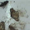
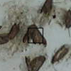
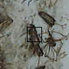
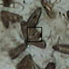
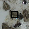
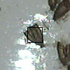
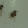
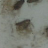
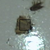
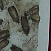
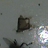
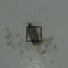
(a) Examples of correct detections

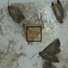
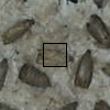
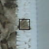
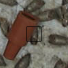
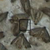
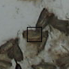
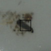
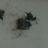
(b) Examples of misdetections

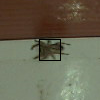
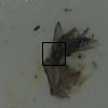
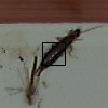
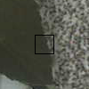
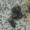
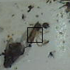
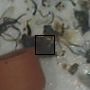
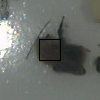
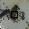
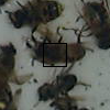
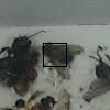
(c) Examples of false positives

Figure 11: Image patches (input + context) of correct detections, misdetections and false positives. Input to the classifier is shown as a black square. Best viewed in colour.

References

- [1] R. T. Carde, A. K. Minks, Control of moth pests by mating disruption: successes and constraints, Annual review of entomology 40 (1) (1995) 559–585.
- [2] P. Witzgall, P. Kirsch, A. Cork, Sex pheromones and their impact on pest management, Journal of chemical ecology 36 (1) (2010) 80–100.
- [3] S.-H. Kang, S.-H. Song, S.-H. Lee, Identification of butterfly species with a single neural network system, Journal of Asia-Pacific Entomology 15 (3) (2012) 431–435.
- [4] S.-H. Kang, J.-H. Cho, S.-H. Lee, Identification of butterfly based on their shapes when viewed from different angles using an artificial neural network, Journal of Asia-Pacific Entomology 17 (2) (2014) 143–149.
- [5] T. Arbuckle, S. Schroder, V. Steinhage, D. Wittmann, Biodiversity informatics in action: identification and monitoring of bee species using abis, in: Proc. 15th Int. Symp. Informatics for Environmental Protection, Vol. 1, Citeseer, 2001, pp. 425–430.
- [6] P. Weeks, M. O’Neill, K. Gaston, I. Gauld, Automating insect identification: exploring the limitations of a prototype system, Journal of Applied Entomology 123 (1) (1999) 1–8.
- [7] A. Tofilski, Drawwing, a program for numerical description of insect wings, Journal of Insect Science 4 (1) (2004) 17.
- [8] J. Wang, C. Lin, L. Ji, A. Liang, A new automatic identification system of insect images at the order level, Knowledge-Based Systems 33 (2012) 102–110.
- [9] N. Larios, H. Deng, W. Zhang, M. Sarpola, J. Yuen, R. Paasch, A. Moldenke, D. A. Lytle, S. R. Correa, E. N. Mortensen, et al., Automated insect identification through concatenated histograms of local appearance features: feature vector generation and region detection for deformable objects, Machine Vision and Applications 19 (2) (2008) 105–123.
- [10] G. Martinez-Munoz, N. Larios, E. Mortensen, W. Zhang, A. Yamamuro, R. Paasch, N. Payet, D. Lytle, L. Shapiro, S. Todorovic, et al., Dictionary-free categorization of very similar objects via stacked evidence trees, in: Computer Vision and Pattern Recognition, 2009. CVPR 2009. IEEE Conference on, IEEE, 2009, pp. 549–556.
- [11] N. Larios, B. Soran, L. G. Shapiro, G. Martínez-Muñoz, J. Lin, T. G. Dietterich, Haar random forest features and svm spatial matching kernel for stonefly species identification., in: ICPR, Vol. 1, 2010, p. 7.
- [12] D. A. Lytle, G. Martínez-Muñoz, W. Zhang, N. Larios, L. Shapiro, R. Paasch, A. Moldenke, E. N. Mortensen, S. Todorovic, T. G. Dietterich, Automated processing and identification of benthic invertebrate samples, Journal of the North American Benthological Society 29 (3) (2010) 867–874.
- [13] S. Al-Saqer, P. Weckler, J. Solie, M. Stone, A. Wayadande, Identification of pecan weevils through image processing, American Journal of Agricultural and Biological Sciences 6 (1) (2010) 69.
- [14] J. Cho, J. Choi, M. Qiao, C.-w. Ji, H.-y. Kim, K.-b. Uhm, T.-s. Chon, Automatic identification of whiteflies, aphids and thrips in greenhouse based on image analysis, Red 346 (246) (2007) 244.
- [15] M. Mayo, A. T. Watson, Automatic species identification of live moths, Knowledge-Based Systems 20 (2) (2007) 195–202.
- [16] Z. Le-Qing, Z. Zhen, Auto-classification of insect images based on color histogram and glcm, in: Fuzzy Systems and Knowledge Discovery (FSKD), 2010 Seventh International Conference on, Vol. 6, IEEE, 2010, pp. 2589–2593.
- [17] Y. Kaya, L. Kayci, Application of artificial neural network for automatic detection of butterfly species using color and texture features, The Visual Computer 30 (1) (2014) 71–79.
- [18] P. Fedor, I. Malenovskỳ, J. Vaňhara, W. Sierka, J. Havel, Thrips (thysanoptera) identification using artificial neural networks, Bulletin of entomological research 98 (05) (2008) 437–447.
- [19] S. N. Yaakob, L. Jain, An insect classification analysis based on shape features using quality threshold artmap and moment invariant, Applied Intelligence 37 (1) (2012) 12–30.
- [20] C. Wen, D. E. Guyer, W. Li, Local feature-based identification and classification for orchard insects, Biosystems engineering 104 (3) (2009) 299–307.
- [21] C. Wen, D. Guyer, Image-based orchard insect automated identification and classification method, Computers and Electronics in Agriculture 89 (2012) 110–115.
- [22] A. Lu, X. Hou, C.-L. Liu, X. Chen, Insect species recognition using discriminative local soft coding, in: Pattern Recognition (ICPR), 2012 21st International Conference on, IEEE, 2012, pp. 1221–1224.
- [23] N. Larios, J. Lin, M. Zhang, D. Lytle, A. Moldenke, L. Shapiro, T. Dietterich, Stacked spatial-pyramid kernel: An object-class recognition method to combine scores from random trees, in: Applications of Computer Vision (WACV), 2011 IEEE Workshop on, IEEE, 2011, pp. 329–335.
- [24] L. Xiao-Lin, H. Shi-Guo, Z. Ming-Quan, G. Guo-Hua, Knn-spectral regression lda for insect recognition, in: Information Science and Engineering (ICISE), 2009 1st International Conference on, IEEE, 2009, pp. 1315–1318.
- [25] I. Zayas, P. Flinn, Detection of insects in bulk wheat samples with machine vision, Transactions of the ASAE-American Society of Agricultural Engineers 41 (3) (1998) 883–888.
- [26] C. Ridgway, E. Davies, J. Chambers, D. Mason, M. Bateman, Rapid machine vision method for the detection of insects and other particulate bio-contaminants of bulk grain in transit, Biosystems engineering 83 (1) (2002) 21–30.
- [27] Y. Qing, L. Jun, Q.-j. LIU, G.-q. DIAO, B.-j. YANG, H.-m. CHEN, T. Jian, An insect imaging system to automate rice light-trap pest identification, Journal of Integrative Agriculture 11 (6) (2012) 978–985.
- [28] Q. Yao, Q. Liu, T. G. Dietterich, S. Todorovic, J. Lin, G. Diao, B. Yang, J. Tang, Segmentation of touching insects based on optical flow and ncuts, Biosystems Engineering 114 (2) (2013) 67–77.
- [29] X. Zhang, Y.-H. Yang, Z. Han, H. Wang, C. Gao, Object class detection: A survey, ACM Computing Surveys (CSUR) 46 (1) (2013) 10.
- [30] A. Andreopoulos, J. K. Tsotsos, 50 years of object recognition: Directions forward, Computer Vision and Image Understanding 117 (8) (2013) 827–891.
- [31] Y. LeCun, L. Bottou, Y. Bengio, P. Haffner, Gradient-based learning applied to document recognition, Proceedings of the IEEE 86 (11) (1998) 2278–2324.
- [32] A. Krizhevsky, I. Sutskever, G. E. Hinton, Imagenet classification with deep convolutional neural networks, in: Advances in neural information processing systems, 2012, pp. 1097–1105.
- [33] D. Ciresan, U. Meier, J. Schmidhuber, Multi-column deep neural networks for image classification, in: Computer Vision and Pattern Recognition (CVPR), 2012 IEEE Conference on, IEEE, 2012, pp. 3642–3649.
- [34] C.-Y. Lee, S. Xie, P. Gallagher, Z. Zhang, Z. Tu, Deeply-supervised nets, arXiv preprint arXiv:1409.5185.
- [35] K. Swersky, J. Snoek, R. P. Adams, Multi-task bayesian optimization, in: Advances in Neural Information Processing Systems, 2013, pp. 2004–2012.
- [36] O. Russakovsky, J. Deng, H. Su, J. Krause, S. Satheesh, S. Ma, Z. Huang, A. Karpathy, A. Khosla, M. Bernstein, et al., Imagenet large scale visual recognition challenge, arXiv preprint arXiv:1409.0575.
- [37] C. Szegedy, W. Liu, Y. Jia, P. Sermanet, S. Reed, D. Anguelov, D. Erhan, V. Vanhoucke, A. Rabinovich, Going deeper with convolutions, arXiv preprint arXiv:1409.4842.
- [38] D. Nikitenko, M. Wirth, K. Trudel, Applicability of white-balancing algorithms to restoring faded colour slides: An empirical evaluation, Journal of Multimedia 3 (5) (2008) 9–18.
- [39] M. Lin, Q. Chen, S. Yan, Network in network, arXiv preprint arXiv:1312.4400.
- [40] A. Krizhevsky, G. Hinton, Learning multiple layers of features from tiny images, Computer Science Department, University of Toronto, Tech. Rep 1 (4) (2009) 7.
- [41] D. Grangier, L. Bottou, R. Collobert, Deep convolutional networks for scene parsing, in: ICML 2009 Deep Learning Workshop, Vol. 3, Citeseer, 2009.
-
[42]
L. Fei-Fei, A. Karpathy, Cs231n:
Convolutional neural networks for visual recognition (2015).
URL http://cs231n.stanford.edu/ - [43] P. F. Felzenszwalb, R. B. Girshick, D. McAllester, D. Ramanan, Object detection with discriminatively trained part-based models, Pattern Analysis and Machine Intelligence, IEEE Transactions on 32 (9) (2010) 1627–1645.
- [44] Y. A. LeCun, L. Bottou, G. B. Orr, K.-R. Müller, Efficient backprop, in: Neural networks: Tricks of the trade, Springer, 2012, pp. 9–48.
- [45] D. E. Rumelhart, G. E. Hinton, R. J. Williams, Learning internal representations by error propagation, Tech. rep., DTIC Document (1985).
- [46] X. Glorot, Y. Bengio, Understanding the difficulty of training deep feedforward neural networks, in: International conference on artificial intelligence and statistics, 2010, pp. 249–256.
- [47] J. Canny, A computational approach to edge detection, Pattern Analysis and Machine Intelligence, IEEE Transactions on (6) (1986) 679–698.
- [48] Y. LeCun, C. Cortes, The mnist database of handwritten digits (1998).
- [49] P. Dollar, C. Wojek, B. Schiele, P. Perona, Pedestrian detection: An evaluation of the state of the art, Pattern Analysis and Machine Intelligence, IEEE Transactions on 34 (4) (2012) 743–761.
- [50] D. G. Lowe, Distinctive image features from scale-invariant keypoints, International journal of computer vision 60 (2) (2004) 91–110.
- [51] J. Wang, Y. Song, T. Leung, C. Rosenberg, J. Wang, J. Philbin, B. Chen, Y. Wu, Learning fine-grained image similarity with deep ranking, in: Computer Vision and Pattern Recognition (CVPR), 2014 IEEE Conference on, IEEE, 2014, pp. 1386–1393.
- [52] A. S. Razavian, H. Azizpour, J. Sullivan, S. Carlsson, Cnn features off-the-shelf: an astounding baseline for recognition, in: Computer Vision and Pattern Recognition Workshops (CVPRW), 2014 IEEE Conference on, IEEE, 2014, pp. 512–519.