The Concentric Maclaurin Spheroid method with tides and a rotational enhancement of Saturn’s tidal response

Abstract

We extend to three dimensions the Concentric Maclaurin Spheroid method for obtaining the self-consistent shape and gravitational field of a rotating liquid planet, to include a tidal potential from a satellite. We exhibit, for the first time, the important effect of the planetary rotation rate on tidal response of gas giants. Simulations of planets with fast rotation rates like those of Jupiter and Saturn, exhibit significant changes in calculated tidal love numbers $k_{nm}$ when compared with non-rotating bodies. A test model of Saturn fitted to observed zonal gravitational multipole harmonics yields $k_{2}=0.413$, consistent with a recent observational determination from Cassini astrometry data [19]. The calculated love number is robust under reasonable assumptions of interior rotation rate, satellite parameters, and details of Saturn’s interior structure. The method is benchmarked against several published test cases.

1 Introduction

The gas giants Jupiter and Saturn rotate so rapidly that adequate treatment of the non-spherical part of their gravitational potential requires either a very high-order perturbative, or better, an entirely non-perturbative approach [11, 12, 10, 23, 24]. Here we present an extension of the Concentric Maclaurin Spheroid (CMS) method of Hubbard [11, 12] to three dimensions to include the tidal perturbation from a satellite. This allows for high-precision simulations of static tidal response, consistent with the planet’s shape and interior mass distribution. The presence of a large rotational bulge produces an observable effect on the tidal response of giant planets. This effect, which has not been previously revealed by linear tidal-response theories applied to spherical-equivalent interior models, has implications for the observed tidal responses of Jupiter and Saturn.

The Juno spacecraft is expected to measure the strength of Jupiter’s gravitational field to an unprecedented precision ($\sim$ one part in $10^{9}$) [16], potentially revealing a weak signal from the planet’s interior dynamics. Also present in Jupiter’s gravitational field will be tesseral-harmonic terms produced by tides raised by the planet’s large satellites. In fact, close to the planet, the gravitational signal from Jupiter’s tides has a similar magnitude to the predicted signal from models of deep internal dynamics [2, 16, 15]. An accurate prediction of the planet’s hydrostatic tidal response will, therefore, be essential for interpreting the high-precision measurements provided by the Juno gravity science experiment.

Although the Cassini Saturn orbiter was not designed for direct measurement of high-order components of Saturn’s gravitational field, it has already provided gravitational information relevant to the planet’s interior structure. Lainey et al. [19] used an astrometry dataset of the orbits of Saturn’s co-orbital satellites to make the first determination of the planet’s $k_{2}$ love number. Their observed $k_{2}$ was significantly larger than the theoretical prediction of Gavrilov and Zharkov [5]. A mismatch between an observed $k_{2}$ and the value predicted for a Saturn model fitted to the planet’s low-degree zonal harmonics $J_{2}$ and $J_{4}$ would raise questions about the adequacy of the hydrostatic (non-dynamic) theory of tides.

In this paper we present theoretical results for simplified Saturn interior models matching the planet’s observed low-degree zonal harmonics. When these models are analyzed with the full 3-d CMS theory including rotation and tides, we predict a gravitational response in line with the observed $k_{2}$ value of Lainey et al. [19], suggesting that the observation can be completely understood in terms of a static tidal response. A similar test will be possible for Jupiter once its $k_{2}$ has been measured by the Juno spacecraft.

There is extensive literature on the problem of the shape and gravitational potential of a liquid planet in hydrostatic equilibrium, responding to its own rotation and to an external gravitational potential from a satellite; see, e.g., a century-old discussion in Jeans [14]. Many classical geophysical investigations use a perturbation approach, obtaining the planet’s linear and higher-order response to small deviations of the potential from spherical symmetry. A good discussion of the application of perturbation theory to rotational response, the so-called theory of figures, is found in Zharkov and Trubitsyn [25], while a pioneering calculation of the tidal response of giant planets is presented by Gavrilov and Zharkov [5].

Hubbard [11] introduced an iterative numerical method, based on the theory of figures, for calculating the self-consistent shape and gravitational field of a constant density, rotating fluid body to high precision. In this method, integrals over the mass distribution are solved using Gaussian quadrature to obtain the gravitational multipole moments. This method was extended to non-constant density profiles by Hubbard [12], by approximating the barotropic pressure-density relationship with multiple concentric Maclaurin (i.e., constant-density) spheroids. This approach (called the CMS method) mitigates problems with cancellation of terms that arise in a purely numerical solution to the general equation of hydrostatic equilibrium, and has a typical relative precision of $\sim 10^{-12}$. The CMS method has been benchmarked against analytical results for simple models [10] and against an independent, non-perturbative numerical method [23, 24].

The theory of Gavrilov and Zharkov [5] begins with an interior model of Saturn fitted to the values of $J_{2}$ and $J_{4}$ observed at that time. This interior model tabulates the mass density $\rho$ as a function of $s$, where $s$ is the mean radius of the constant-density surface. Tidal perturbation theory is then applied to this spherical-equivalent Saturn. The Gavrilov and Zharkov [5] approach is sufficient for an initial estimate of the tidally-induced terms in the external potential, but it neglects terms which are of the order of the product of the tidal perturbation and the rotational perturbation. Here we demonstrate that, for a rapidly-rotating giant planet, the latter terms make a significant contribution to the love numbers $k_{nm}$, as well as (unobservably small) tidal contributions to the gravitational moments $J_{n}$.

Folonier et al. [4] presented a method for approximating the love numbers of a non-homogeneous body using Clairaut theory for the equilibrium ellipsoidal figures. This results in an expression for the love number $k_{2}$ for a body composed of concentric ellipsoids, parameterized by their flattening parameters. In the case of the constant density Maclaurin spheroid, there is a well-known result that the equipotential surface is an ellipsoid. However, in bodies with more complicated density distributions, the equipotential surfaces will have a more general spheroidal shape. Because of the small magnitude of tidal perturbations, the method of Folonier et al. [4] works in the limit of slow rotation despite this limitation. However, the method does not account for the coupled effect of tides and rotation, and does not predict love numbers of order higher than $k_{2}$. Within these constraints, we show below that our extended CMS method yields results that are in excellent agreement with results from Folonier et al. [4].

Although our theory is quite general and can be used to calculate a rotating planet’s tidal response to multiple satellites located at arbitrary latitudes, longitudes, and radial distances, for application to Jupiter and Saturn it suffices to consider the effect of a single perturbing satellite sitting on an orbital plane at zero inclination to the planet’s equator. Since tidal distortions are always very small compared with rotational distortion, and Jupiter’s Galilean satellites, as well many of Saturn’s larger satellites, are on orbits with low inclination, the tidal response to multiple satellites can be obtained by a linear superposition of the perturbation from each body. Extension of our theory to a system with a large satellite on an inclined orbit, such as Neptune-Triton, would be straightforward, but is not considered here.

2 Concentric Maclaurin Spheroid method with tides

2.1 Model parameters

In the co-rotating frame of the planet in hydrostatic equilibrium, the pressure $P$, the mass density $\rho$ and the total effective potential $U$ are related by

$$\nabla P=\rho\nabla U.$$ (1)

The total effective potential can be separated into three components,

$$U=V+Q+W,$$ (2)

where $V$ is the gravitational potential arising from the mass distribution within the planet, $Q$ is the centrifugal potential corresponding to a rotation frequency $\omega$, and $W$ is the tidal potential arising from a satellite with mass $m_{\rm s}$ at planet-centered coordinates $(R,\mu_{s},\phi_{s})$, where $R$ is the satellite’s orbital distance from the origin, $\mu_{s}=\cos\theta$, where $\theta$ is the satellite’s planet-centered colatitude and $\phi_{s}$ is the planet-centered longitude. For the purposes of this investigation, we always place the satellite at angular coordinates $\mu_{s}=0$ and $\phi_{s}=0$. The relative magnitudes of $V$, $Q$, and $W$ can be described in terms of two non-dimensional numbers:

$$q_{\rm rot}=\frac{\omega^{2}a^{3}}{GM}$$ (3)

for the rotational perturbation and

$$q_{\rm tid}=-\frac{3m_{\rm s}a^{3}}{MR^{3}}$$ (4)

for the tidal perturbation, where $G$ is the universal gravitational constant, and $M$ and $a$ are the mass and equatorial radius of the planet. The planet-satellite system is described by these two small parameters along with a third parameter, the ratio $a/R$.

Since CMS theory is nonperturbative, in principle our results are valid to all powers of these small parameters and their products (until we reach the computer’s numerical precision limit). For the giant-planet tidal problems that we consider here, terms of second and higher order in $q_{\rm tid}$ are always negligible, but terms linear in $q_{\rm tid}$ and multiplied by various powers of $q_{\rm rot}$ and $a/R$ contribute above the numerical noise level. It is, in fact, terms of order $q_{\rm tid}\cdot q_{\rm rot}$ that contribute most importantly to the new results of this paper.

We introduce dimensionless planetary units of pressure $P_{\rm pu}$, density $\rho_{\rm pu}$, and total potential $U_{\rm pu}$, such that

$$P\equiv \frac{GM^{2}}{a^{4}}P_{\rm pu}$$ (5)

$$\rho\equiv \frac{M}{a^{3}}\rho_{\rm pu}$$

$$U\equiv \frac{GM}{a}U_{\rm pu}.$$

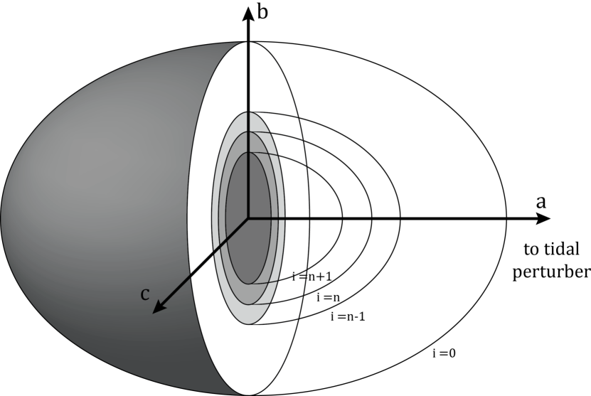
Figure 1: Conceptual diagram of a Concentric Maclaurin Spheroid model with a tidal perturbation from a satellite.

The CMS method considers a model planet composed of $N$ nested spheroids of constant density as depicted in Figure 1. We label these spheroids with index $i=0,1,2,\dots,N-1$, with $i=0$ corresponding to the outermost spheroid and $i=N-1$ corresponding to the innermost spheroid. Each spheroid is constrained to have a point at radial distance $a_{i}$ from the planet’s center of mass, such that each of these fixed points has the same angular coordinates as the sub-satellite point $(\mu=0,\phi=0)$. Accordingly, the $a_{0}$ of the outermost spheroid corresponds to its the largest principal axis, if the perturbing satellite is in the equatorial plane.

When $q_{\rm tid}=0$, the potential is axially symmetric and the problem can be solved in two spatial dimensions. However, when both $q_{\rm tid}$ and $q_{\rm rot}$ are nonzero, the symmetry is broken, meaning that each spheroid has a fully triaxial figure with the surface described by

$$\zeta_{i}\equiv r_{i}(\mu,\phi)/a_{i},$$ (6)

such that $\zeta_{0}$ represents the shape of the outer surface.

Taking advantage of the principle of superposition for a linear relationship between the potential $V$ and the mass density $\rho$, the total $V$ is given by the sum of the potential arising from each individual spheroid [12]. This allows us to approximate any monotonically increasing density profile, with the density of the $i$th spheroid represented by the density jump

$$\delta\rho_{i}=\begin{cases}\rho_{i}-\rho_{i-1},&i>0\\ \rho_{0},&i=0.\end{cases}$$ (7)

This parameterization of density has the added benefit of naturally handling discontinuities in $\rho$, as would be expected for a giant planet with a dense central core.

2.2 Calculation of gravitational potential

The general expansion of $V$ in spherical coordinates ${\bf r}=(r,\mu=\cos{\theta},\phi)$ is

$$V (r,\mu,\phi)=$$ (8)

$$\frac{GM}{r}\left[\sum_{n=0}^{\infty}P_{n}(\mu)\int_{\tau}d\tau\rho(r^{\prime})P_{n}(\mu^{\prime})\left(\frac{r^{\prime}}{r}\right)^{k}\right.$$

$$+\sum_{n=0}^{\infty}\sum_{m=1}^{n}P^{m}_{n}(\mu)\cos(m\phi)\int_{\tau}d\tau\frac{2(n-m)!}{(n+m)!}\rho(r^{\prime})P_{n}^{m}(\mu^{\prime})\cos(m\phi^{\prime})\left(\frac{r^{\prime}}{r}\right)^{k}$$

$$\left.+\sum_{n=0}^{\infty}\sum_{m=1}^{n}P^{m}_{n}(\mu)\sin(m\phi)\int_{\tau}d\tau\frac{2(n-m)!}{(n+m)!}\rho(r^{\prime})P_{n}^{m}(\mu^{\prime})\sin(m\phi^{\prime})\left(\frac{r^{\prime}}{r}\right)^{k}\right]$$

[25], where $P_{n}$ and $P_{n}^{m}$ are the Legendre and associated Legendre polynomials,

$$d\tau=r^{\prime 2}\sin(\theta^{\prime})d\theta^{\prime}d\phi^{\prime}=r^{\prime 2}d\mu^{\prime}d\phi^{\prime},$$

and the origin, ${\bf r}=(0,0,0)$, is the center of mass of the planet. The potential at a general point within the planet has a contribution from mass both interior and exterior to that point, for which the exponent $k$ in Eqn. (8) is different:

$$k=\begin{cases}n,&r^{\prime}<r\\ -(n+1),&r^{\prime}>r.\end{cases}$$

The centrifugal potential $Q$ depends only on $r$ and $\mu$

$$Q(r,\mu)=\frac{1}{3}r^{2}\omega^{2}\left[1-P_{2}(\mu)\right].$$ (9)

The tidal potential $W$ for a satellite at position ${\bf R}=(R,\mu_{s},\phi_{s})$ is

$$W({\bf r})=\frac{Gm_{\rm s}}{\left|{\bf R}-{\bf r}\right|}.$$ (10)

The general expansion of $W$ around the center of mass of the planet is obtained by using the summation theorem for spherical harmonics [5]

$$W(r,\mu,\phi)= \frac{Gm_{\rm s}}{R}\sum_{n=0}^{\infty}\left[P_{n}(\mu)P_{n}(\mu_{s})\phantom{\frac{1}{1}}\right.$$ (11)

$$\left.+2\sum_{m=1}^{n}\frac{2(n-m)!}{(n+m)!}\cos(m\phi-m\phi_{s})P_{n}^{m}(\mu)P_{n}^{m}(\mu_{s})\right].$$

Following Hubbard [12], we derive non-dimensional quantities in terms of the planet mass $M$ and maximum radius $a=a_{0}$. For each spheroid, we define a dimensionless radius of each spheroid

$$\lambda_{i}\equiv a_{i}/a$$ (12)

and dimensionless density increment, based on the mean density of the planet

$$\bar{\rho}= \frac{3M}{a^{3}}\frac{1}{\int_{-1}^{1}d\mu^{\prime}\int_{0}^{2\pi}d\phi^{\prime}\zeta_{0}^{3}}$$ (13)

$$\delta_{i}\equiv \frac{\delta\rho_{i}}{\bar{\rho}}.$$

The model planet’s mass is then given by the integral expression

$$M=\frac{1}{3}\sum_{j=0}^{N-1}\delta_{j}\lambda_{j}^{3}\int_{-1}^{1}d\mu^{\prime}\int_{0}^{2\pi}d\phi^{\prime}\zeta_{j}^{3}.$$ (14)

The contribution to the potential is expanded in terms of interior and external zonal harmonics $J_{i,n}$ and $J_{i,n}^{\prime}$. For the tidal problem, we must also consider the analogous $C_{i,nm}$, $C^{\prime}_{i,nm}$, $S_{i,nm}$ and $S^{\prime}_{i,nm}$. These contribute linearly to the total moment evaluated exterior to the planet’s surface; for instance,

$$J_{2}=\sum_{i=0,N-1}J_{i,2}.$$ (15)

The layer-specific harmonics are then normalized by radius as

$$\widetilde{J}_{i,n}\equiv \frac{J_{i,n}}{\lambda_{i}^{n}}, \widetilde{J}^{\prime}_{i,n}\equiv J^{\prime}_{i,n}\lambda_{i}^{(n+1)}$$ (16)

$$\widetilde{S}_{i,nm}\equiv \frac{S_{i,nm}}{\lambda_{i}^{n}}, \widetilde{S}^{\prime}_{i,nm}\equiv S^{\prime}_{i,nm}\lambda_{i}^{(n+1)}$$

$$\widetilde{C}_{i,nm}\equiv \frac{C_{i,nm}}{\lambda_{i}^{n}}, \widetilde{C}^{\prime}_{i,nm}\equiv C^{\prime}_{i,nm}\lambda_{i}^{(n+1)}.$$

Following the derivation in Hubbard [12] and generalizing the expressions for full three dimensional volume integrals, we find the normalized interior harmonics

$$\widetilde{J}_{i,n} = -\frac{3}{n+3}\frac{\delta_{i}\lambda_{i}^{3}\int_{-1}^{1}d\mu^{\prime}P_{n}(\mu^{\prime})\int_{0}^{2\pi}d\phi^{\prime}\zeta_{i}^{(n+3)}}{\sum_{j=0}^{N-1}\delta_{j}\lambda_{j}^{3}\int_{-1}^{1}d\mu^{\prime}\int_{0}^{2\pi}d\phi^{\prime}\zeta_{j}^{3}}$$ (17)

$$\widetilde{C}_{nm} = \frac{6(n-m)!}{(n+3)(n+m)!}\frac{\delta_{i}\lambda_{i}^{3}\int_{-1}^{1}d\mu^{\prime}P_{n}^{m}(\mu^{\prime})\int_{0}^{2\pi}d\phi^{\prime}\zeta_{i}^{(n+3)}\cos(m\phi^{\prime})}{\sum_{j=0}^{N-1}\delta_{j}\lambda_{j}^{3}\int_{-1}^{1}d\mu^{\prime}\int_{0}^{2\pi}d\phi^{\prime}\zeta_{j}^{3}}$$

$$\widetilde{S}_{nm} = \frac{6(n-m)!}{(n+3)(n+m)!}\frac{\delta_{i}\lambda_{i}^{3}\int_{-1}^{1}d\mu^{\prime}P_{n}^{m}(\mu^{\prime})\int_{0}^{2\pi}d\phi^{\prime}\zeta_{i}^{(n+3)}\sin(m\phi^{\prime})}{\sum_{j=0}^{N-1}\delta_{j}\lambda_{j}^{3}\int_{-1}^{1}d\mu^{\prime}\int_{0}^{2\pi}d\phi^{\prime}\zeta_{j}^{3}},$$

and the exterior harmonics

$$\widetilde{J}^{\prime}_{i,n} = -\frac{3}{2-n}\frac{\delta_{i}\lambda_{i}^{3}\int_{-1}^{1}d\mu^{\prime}P_{n}(\mu^{\prime})\int_{0}^{2\pi}d\phi^{\prime}\zeta_{i}^{(-n+2)}}{\sum_{j=0}^{N-1}\delta_{j}\lambda_{j}^{3}\int_{-1}^{1}d\mu^{\prime}\int_{0}^{2\pi}d\phi^{\prime}\zeta_{j}^{3}}$$ (18)

$$\widetilde{C}^{\prime}_{nm} = \frac{6(n-m)!}{(2-n)(n+m)!}\frac{\delta_{i}\lambda_{i}^{3}\int_{-1}^{1}d\mu^{\prime}P_{n}^{m}(\mu^{\prime})\int_{0}^{2\pi}d\phi^{\prime}\zeta_{i}^{(-n+2)}\cos(m\phi^{\prime})}{\sum_{j=0}^{N-1}\delta_{j}\lambda_{j}^{3}\int_{-1}^{1}d\mu^{\prime}\int_{0}^{2\pi}d\phi^{\prime}\zeta_{j}^{3}}$$

$$\widetilde{S}^{\prime}_{nm} = \frac{6(n-m)!}{(2-n)(n+m)!}\frac{\delta_{i}\lambda_{i}^{3}\int_{-1}^{1}d\mu^{\prime}P_{n}^{m}(\mu^{\prime})\int_{0}^{2\pi}d\phi^{\prime}\zeta_{i}^{(-n+2)}\sin(m\phi^{\prime})}{\sum_{j=0}^{N-1}\delta_{j}\lambda_{j}^{3}\int_{-1}^{1}d\mu^{\prime}\int_{0}^{2\pi}d\phi^{\prime}\zeta_{j}^{3}}$$

with a special case for $n=2$

$$\widetilde{J}^{\prime}_{i,n} = -3\frac{\delta_{i}\lambda_{i}^{3}\int_{-1}^{1}d\mu^{\prime}P_{n}(\mu^{\prime})\int_{0}^{2\pi}d\phi^{\prime}\log(\zeta_{i})}{\sum_{j=0}^{N-1}\delta_{j}\lambda_{j}^{3}\int_{-1}^{1}d\mu^{\prime}\int_{0}^{2\pi}d\phi^{\prime}\zeta_{j}^{3}}$$ (19)

$$\widetilde{C}^{\prime}_{nm} = \frac{6(n-m)!}{(n+m)!}\frac{\delta_{i}\lambda_{i}^{3}\int_{-1}^{1}d\mu^{\prime}P_{n}^{m}(\mu^{\prime})\int_{0}^{2\pi}d\phi^{\prime}\log(\zeta_{i})\cos(m\phi^{\prime})}{\sum_{j=0}^{N-1}\delta_{j}\lambda_{j}^{3}\int_{-1}^{1}d\mu^{\prime}\int_{0}^{2\pi}d\phi^{\prime}\zeta_{j}^{3}}$$

$$\widetilde{S}^{\prime}_{nm} = \frac{6(n-m)!}{(n+m)!}\frac{\delta_{i}\lambda_{i}^{3}\int_{-1}^{1}d\mu^{\prime}P_{n}^{m}(\mu^{\prime})\int_{0}^{2\pi}d\phi^{\prime}\log(\zeta_{i})\sin(m\phi^{\prime})}{\sum_{j=0}^{N-1}\delta_{j}\lambda_{j}^{3}\int_{-1}^{1}d\mu^{\prime}\int_{0}^{2\pi}d\phi^{\prime}\zeta_{j}^{3}}$$

and

$$J^{\prime\prime}_{i,0}= \frac{2\pi\delta_{i}a_{0}^{3}}{3M}.$$ (20)

The shape of the surface of the planet is defined by the equipotential relationship

$$U(\zeta,\mu,\phi,\mu_{s},\phi_{s})-U(1,0,0,\mu_{s},\phi_{s})=0,$$ (21)

where the potential in planetary units at an arbitrary point on the planet’s surface

$$U(\zeta,\mu,\phi,\mu_{s},\phi_{s})= \frac{1}{\zeta_{0}}\left[1-\sum^{N-1}_{i=0}\sum^{\infty}_{n=1}\lambda_{i}^{n}\zeta_{0}^{-n}\left\{P_{n}(\mu)\widetilde{J}_{i,n}\phantom{\sum_{1}^{n}}\right.\right.$$ (22)

$$\left.-\sum_{m=1}^{n}P_{n}^{m}(\mu)\left(\widetilde{C}_{i,nm}\cos(m\phi)+\widetilde{S}_{i,nm}\sin(m\phi)\right)\right\}$$

$$+\frac{1}{3}q_{\rm rot}\zeta_{0}^{3}[1-P_{2}(\mu)]$$

$$-\frac{1}{3}\zeta_{0}^{3}q_{\rm tid}\sum_{n=2}^{\infty}\left(\frac{a}{R}\right)^{(n-2)}\zeta_{0}^{(n-2)}\left\{P_{n}(\mu)P_{n}(\mu_{s})\phantom{\sum_{1}^{n}}\right.$$

$$\left.\left.+2\sum_{m=1}^{n}\frac{(n-m)!}{(n+m)!}\cos(m\phi-m\phi_{s})P_{n}^{m}(\mu)P_{n}^{m}(\mu_{s})\right\}\right]$$

matches the reference potential at the sub-satellite point

$$U(1,0,0,\mu_{s},\phi_{s})= 1-\sum^{N-1}_{i=0}\sum^{\infty}_{n=1}\lambda_{i}^{n}\left\{P_{n}(0)\widetilde{J}_{i,n}-\sum_{m=1}^{n}P_{n}^{m}(0)\widetilde{C}_{i,nm}\right\}$$ (23)

$$+\frac{1}{2}q_{\rm rot}-\frac{1}{3}q_{\rm tid}\sum_{n=2}^{\infty}\left(\frac{a}{R}\right)^{(n-2)}\left\{P_{n}(0)P_{n}(\mu_{s})\phantom{\sum_{a}^{b}}\right.$$

$$\left.+2\sum_{m=1}^{n}\frac{(n-m)!}{(n+m)!}\cos(-m\phi_{s})P_{n}^{m}(0)P_{n}^{m}(\mu_{s})\right\}.$$

Similarly, the shapes of the interior spheroids are found by solving

$$U_{j}(\zeta,\mu,\phi,\mu_{s},\phi_{s})-U_{j}(1,0,0,\mu_{s},\phi_{s})=0,$$ (24)

where

$$U_{j}(\zeta_{j},\mu,\phi,\mu_{s},\phi_{s})= -\frac{1}{\zeta_{j}\lambda_{j}}\left[\sum^{N-1}_{i=j}\sum^{\infty}_{n=0}\left(\frac{\lambda_{i}}{\lambda_{j}}\right)^{n}\zeta_{j}^{-n}\left\{P_{n}(\mu)\widetilde{J}_{i,n}\phantom{\sum_{a}^{b}}\right.\right.$$ (25)

$$\left.-\sum_{m=1}^{n}P_{n}^{m}(\mu)\left(\widetilde{C}_{i,nm}\cos(m\phi)+\widetilde{S}_{i,nm}\sin(m\phi)\right)\right\}$$

$$+\sum^{j-1}_{i=0}\sum^{\infty}_{n=0}\left(\frac{\lambda_{j}}{\lambda_{i}}\right)^{n+1}\zeta_{j}^{n+1}\left\{\widetilde{J}^{\prime}_{i,n}P_{n}(\mu)\phantom{\sum_{1}^{m}}\right.$$

$$\left.-\sum_{m=1}^{n}P_{n}^{m}(\mu)\left(\widetilde{C}^{\prime}_{i,nm}\cos(m\phi)+\widetilde{S}^{\prime}_{i,nm}\sin(m\phi)\right)\right\}$$

$$+\left.\sum^{j-1}_{i=0}J^{\prime\prime}_{i,0}\lambda_{j}^{3}\zeta_{j}^{3}\right]+\frac{1}{3}q_{\rm rot}\lambda_{j}^{2}\zeta_{j}^{2}[1-P_{2}(\mu)]$$

$$-\frac{1}{3}\lambda_{j}^{2}\zeta_{j}^{2}q_{\rm tid}\sum_{n=2}^{\infty}\left(\frac{a\lambda_{j}}{R}\right)^{(n-2)}\zeta_{j}^{(n-2)}\left\{P_{n}(\mu)P_{n}(\mu_{s})\phantom{\sum_{a}^{b}}\right.$$

$$\left.+2\sum_{m=1}^{n}\frac{(n-m)!}{(n+m)!}\cos(m\phi-m\phi_{s})P_{n}^{m}(\mu)P_{n}^{m}(\mu_{s})\right\}$$

and

$$U_{j}(1,0,0,\mu_{s},\phi_{s})= -\frac{1}{\lambda_{j}}\left[\sum^{N-1}_{i=j}\sum^{\infty}_{n=0}\left(\frac{\lambda_{i}}{\lambda_{j}}\right)^{n}\left\{P_{n}(0)\widetilde{J}_{i,n}-\sum_{m=1}^{n}P_{n}^{m}(0)\widetilde{C}_{i,nm}\right\}\right.$$ (26)

$$+\sum^{j-1}_{i=0}\sum^{\infty}_{n=0}\left(\frac{\lambda_{j}}{\lambda_{i}}\right)^{n+1}\left\{\widetilde{J}^{\prime}_{i,n}P_{n}(0)-\sum_{m=1}^{n}P_{n}^{m}(0)\widetilde{C}^{\prime}_{i,nm}\right\}$$

$$\left.+\sum^{j-1}_{i=0}J^{\prime\prime}_{i,0}\lambda_{j}^{3}\right]+\frac{1}{2}q_{\rm rot}\lambda_{j}^{2}$$

$$-\frac{1}{3}\lambda_{j}^{2}q_{\rm tid}\sum_{n=2}^{\infty}\left(\frac{a\lambda_{j}}{R}\right)^{(n-2)}\left\{P_{n}(0)P_{n}(\mu_{s})\phantom{\sum_{1}^{1}}\right.$$

$$\left.+2\sum_{m=1}^{n}\frac{(n-m)!}{(n+m)!}\cos(-m\phi_{s})P_{n}^{m}(0)P_{n}^{m}(\mu_{s})\right\}.$$

From Eqn. (26), we also find the potential at the center of the planet

$$U_{\rm center}=-\sum_{i=0}^{N-1}\sum_{n=0}^{\infty}\lambda_{i}\left\{\widetilde{J}^{\prime}_{i,n}-\sum_{m=1}^{n}\widetilde{C}^{\prime}_{i,nm}\right\}.$$ (27)

Taking the limit of Eqn. (27) as the radius goes to zero yields

$$U_{\rm center} =\lim_{\zeta_{j}\to 0}U_{j}(\zeta_{j})$$ (28)

$$=-\sum_{i=0}^{N-1}\frac{J^{\prime}_{i,n=0}}{\lambda_{i}},$$

correcting a typographical error in Eqn. 49 of Hubbard [12]. In solving equations (21) and (24), we also require their analytical derivatives

$$\frac{d\left[U(\zeta,\mu,\phi,\mu_{s},\phi_{s})-U(1,0,0,\mu_{s},\phi_{s})\right]}{d\zeta}= \frac{dU(\zeta,\mu,\phi)}{d\zeta}$$ (29)

$$\frac{d\left[U_{j}(\zeta_{j},\mu,\phi,\mu_{s},\phi_{s})-U_{j}(1,0,0,\mu_{s},\phi_{s})\right]}{d\zeta_{j}}= \frac{dU_{j}(\zeta_{j},\mu,\phi)}{d\zeta_{j}}.$$

2.3 Gaussian quadrature

The preceding expressions give the gravitational potential and equipotential shapes, as a function of $q_{\rm rot}$ and $q_{\rm tid}$, within a layered planet with $N$ concentric spheroids. In the limit of $N\to\infty$, the solution would apply to an arbitrary monotonically increasing barotropic relation, $\rho(P)$.

For practical applications, we need to find the potential as a multipole expansion up to a maximum degree $n_{\max}$. For the results presented here, we use $n_{\max}=30$. The angular integrals in equations (17) – (19) can be evaluated using Gaussian quadratures on a two dimensional grid. Here we use Legendre-Gauss integration to integrate polar angles over $L_{1}=48$ quadrature points $\mu_{\alpha}=\cos(\theta_{\alpha})$, $\alpha=1,2,\dots L_{1}$, with the corresponding weights $\omega_{\alpha}$, $\alpha=1,2,\dots L_{1}$ over the interval $0<\mu<1$. At any point in the calculation, we must keep track of radius values for each layer on a 2D grid of quadrature points $\zeta_{i\alpha\beta}$. For efficiency, we precalculate the values of all of the Legendre and associated Legendre polynomials at each polar quadrature point, $P_{n}(\mu_{\alpha})$ and $P_{n}^{m}(\mu_{\alpha})$.

For the azimuthal angle, we encounter integrals of the form

$$I_{c,m}\equiv\int^{2\pi}_{0}f(\phi)\cos(m\phi)d\phi$$ (30)

$$I_{s,m}\equiv\int^{2\pi}_{0}f(\phi)\sin(m\phi)d\phi$$

when calculating the tesseral harmonics. For these, we use Chebyshev-Gauss integration with $L_{2}=96$ quadrature points $\eta_{\beta}=\cos(\phi_{\beta})$, $\beta=1,2,\dots L_{2}$, with the corresponding weights $\omega_{\beta}$, $\beta=1,2,\dots L_{2}$ over the interval $0<\phi<2\pi$

$$d\eta=-\sin(\phi)d\phi$$ (31)

$$d\phi=-\frac{d\eta}{\sqrt{1-\eta^{2}}}.$$

Using the identity $(\sin\theta)^{m-k}=(1-\mu^{2})^{\frac{m-k}{2}}$, the sinusoidal functions can be expanded as

$$\cos{m\phi}=\sum^{m}_{k=0}{m\choose k}\eta^{k}(1-\eta^{2})^{\frac{m-k}{2}}\cos\left\{\frac{\pi}{2}(m-k)\right\}$$ (32)

$$\sin{m\phi}=\sum^{m}_{k=0}{m\choose k}\eta^{k}(1-\eta^{2})^{\frac{m-k}{2}}\sin\left\{\frac{\pi}{2}(m-k)\right\}.$$

Substituting these into Eqn. (30) and splitting the integral into two intervals $0<\phi<\pi$ and $\pi<\phi<2\pi$ yields

$$I_{c,m}= \sum^{m}_{k=0}{m\choose k}\cos\left[\frac{\pi}{2}(m-k)\right]\left\{\int^{1}_{-1}\eta^{k}f(\cos^{-1}(-\eta))\left[1-\eta^{2}\right]^{\frac{m-k}{2}}d\eta\right.$$ (33)

$$-\left.\int^{1}_{-1}\eta^{k}f(\cos^{-1}\eta)\left[1-\eta^{2}\right]^{\frac{m-k}{2}}d\eta\right\}$$

$$= \sum^{m}_{k=0}{m\choose k}\cos\left[\frac{\pi}{2}(m-k)\right]$$

$$*\left\{\pm\sum^{L_{2}}_{\beta=1}\omega_{\beta}\eta_{\beta}^{k}f(\pi-\cos^{-1}(\eta_{\beta}))\left[1-\eta_{\beta}^{2}\right]^{\frac{m-k}{2}}\right.$$

$$-\left.\sum^{L_{2}}_{\beta=1}\omega_{\beta}\eta_{\beta}^{k}f(\cos^{-1}\eta_{\beta})\left[1-\eta_{\beta}^{2}\right]^{\frac{m-k}{2}}\right\},$$

where the sign of the second sum depends on the parity of $m$. When calculating the zonal harmonics, the integral $I_{c,m}(f(\mu_{\alpha},\phi_{\beta}))$ reduces to the axisymmetric solution with $m=0$. The zonal harmonics Eqn. (17) can, therefore, be calculated via the summation

$$\widetilde{J}_{i,n}\approx-\left(\frac{3}{n+3}\right)\left(\frac{\delta_{i}\lambda_{i}^{3}\sum^{L_{1}}_{\alpha=1}\omega_{\alpha}P_{n}(\mu_{\alpha})I_{c,0}(\zeta_{i\alpha\beta}^{(n+3)})}{\sum_{j=0}^{N-1}\delta_{j}\lambda_{j}^{3}\sum^{L_{1}}_{\alpha=1}\omega_{\alpha}I_{c,0}(\zeta_{j\alpha\beta}^{3})}\right)$$ (34)

and the tesseral harmonics likewise via

$$\widetilde{C}_{nm} \approx \frac{6(n-m)!}{(n+3)(n+m)!}\left(\frac{\delta_{i}\lambda_{i}^{3}\sum^{L_{1}}_{\alpha=1}\omega_{\alpha}P^{m}_{n}(\mu_{\alpha})I_{c,m}(\zeta_{i\alpha\beta}^{(n+3)})}{\sum_{j=0}^{N-1}\delta_{j}\lambda_{j}^{3}\sum^{L_{1}}_{\alpha=1}\omega_{\alpha}I_{c,0}(\zeta_{j\alpha\beta}^{3})}\right).$$ (35)

There are analogous expressions for $I_{s,m}$ and $S_{nm}$, but these evaluate to zero in all calculations presented here due to the symmetry of the model.

2.4 Iterative procedure

We begin with initial estimates for the shape of each surface $\zeta_{i\alpha\beta,0}$ and for the moments $\widetilde{J}_{i,n}$, $\widetilde{J}^{\prime}_{i,n}$, $\widetilde{J}^{\prime\prime}_{i}$, $\widetilde{C}_{i,nm}$, $\widetilde{C}^{\prime}_{i,nm}$, $\widetilde{S}_{i,nm}$, and $\widetilde{S}^{\prime}_{i,nm}$. For each iteration $t$ the level surfaces are then updated using a single Newton-Raphson integration step.

$$\zeta_{i\alpha\beta,t+1}=\zeta_{i\alpha\beta,t}-\frac{f(\zeta_{i\alpha\beta,t})}{f^{\prime}(\zeta_{i\alpha\beta,t})}$$ (36)

where $f$ is the equipotential relation, Equations (21) – (23) for the outermost surface and Equations (24) – (26) for interior layers, and $f^{\prime}$ is the first derivative of that function with respect to $\zeta$, Eqn. (29). The multipole moments are then calculated for the updated $\zeta_{i\alpha\beta}$ via Equations (17) – (19). These two steps are repeated until all of the exterior moments, $J_{n}$, $C_{nm}$ and $S_{nm}$, have converged such that the difference between successive iterations falls below a specified tolerance. Starting with a naive guess for the initial state, a typical calculation achieves a precision much higher than would be required for comparison with Juno measurements after about 40 iterations.

In simulations with a finite $q_{\rm rot}$ and $q_{\rm tid}$, we typically find an initial converged equilibrium shape with a non-zero, first-order harmonic coefficient $C_{11}$ of the order of $q_{\rm rot}\cdot q_{\rm tid}$ or smaller. This indicates that the center of mass of the system is shifted slightly along the planet-satellite axis from the origin of the initial coordinate system. To remove this term, we apply a translation to the shape function of $\Delta x=-a\cdot C_{11}$ in the direction of the satellite. This correction requires approximating the coordinates $(\mu^{\prime},\phi^{\prime})$ in the uncorrected frame that correspond to the quadrature points $\mu_{\alpha}$ and $\phi_{\beta}$ in the corrected frame, so that the correct shape $\zeta$ is integrated to find the moments in the corrected frame. For a value of $q_{\rm tid}$ similar to the gas giants, this correction yields a body with $C_{11}$ on the order of the specified tolerance. For systems with a much larger $q_{\rm tid}$ (of which there are none in our planetary system), this second-order effect might affect the precision of the calculation. The residual effect is below the numerical noise level for the Saturn models presented in this paper.

2.5 Calculation of the barotrope

We first calculate the density of each uniform layer; for the $j$th layer we have

$$\rho_{j,{\rm pu}}=\frac{\sum_{i=0}^{j}\delta_{i}}{\sum_{k=0}^{N-1}\delta_{k}\lambda_{k}^{3}\int_{-1}^{1}d\mu^{\prime}\int_{0}^{2\pi}d\phi^{\prime}\zeta_{k}^{3}}.$$ (37)

Using this expression, we calculate the total potential $U_{\rm pu}$ on the surface of each layer and at the center using Equations (23) and (26) – (27). Since the density is constant between interfaces, the hydrostatic equilibrium relation, Eqn. (1) is trivially integrated to obtain the pressure at the bottom of the $j$th layer.

$$P_{j,{\rm pu}}=P_{j-1,{\rm pu}}+\rho_{j-1,{\rm pu}}(U_{j,{\rm pu}}-U_{j-1,{\rm pu}})$$ (38)

After obtaining a converged hydrostatic-equilibrium model for N spheroids with the above array using the initial density profile $\delta_{j}$, one calculates the arrays $U_{j,{\rm pu}}$ and $P_{j,{\rm pu}}$. Next, one calculates an array of desired densities

$$\rho_{j,{\rm pu},{\rm desired}}=\rho\left(\frac{1}{2}(P_{j+1}+P_{j})\right),$$ (39)

where $\rho(P)$ is the inverse of the adopted barotrope $P(\rho)$. Finding the difference between the desired densities of subsequent layers then gives a new array of $\delta_{j}$ for use in the next iteration. In our implementation, it is also necessary to scale these densities by a constant factor to obtain the correct total mass of the CMS model.

Self-gravity from the model’s rotational and tidal deformation will cause a small change in the density profile from that expected for a spherical body. In practice, only relatively large changes in the shape of the body will cause a significant deviation in the density profile. Since $q_{\rm rot}\gg q_{\rm tid}$, the influence of rotation dominates the shape of the body. For this reason, we can use an axisymmetric, rotation-only model as described in Hubbard [12] to find a converged density structure for a given barotrope and specified $q_{\rm rot}$, and then perform a single further iteration with tides added to find the hydrostatic solution for that density profile. Because the tide-induced density changes are very small, it is unnecessary to iterate with Eqn. (39) to relax the configuration further for the triaxial figure. Converging the density-pressure profile to a prescribed barotrope and a fully triaxial figure with relatively large $q_{\rm tid}$ is significantly more computationally expensive, and is irrelevant to any giant planet in our planetary system.

3 Comparison with test cases

3.1 Single Maclaurin spheroid

The well-known special case of a single constant-density Maclaurin spheroid is an important test, because it has a closed form, analytical solution to the theory of figures [22]. In equilibrium, the Maclaurin spheroid will have an ellipsoidal shape. In the limit of a low-amplitude tidal perturbation and zero rotation, the love number for all permitted $n$ is

$$k_{n}=\frac{3}{2(n-1)}$$ (40)

[20].

From our simulation results, we calculate the love numbers as

$$k_{nm}=-\frac{2}{3}\frac{(n+m)!}{(n-m)!}\frac{C_{nm}}{P_{n}^{m}(0)q_{\rm tid}}\left(\frac{a}{R}\right)^{2-n}.$$ (41)

For simulations with finite $q_{\rm tid}$ and $q_{\rm rot}=0$, we find our calculated $k_{nm}$ to be degenerate with $m$ in accordance with the analytical result. For a given value of $n$,

$$k_{nm}=\begin{cases}0,&n\mathrm{~{}and~{}}m\mathrm{~{}opposite~{}parity}\\ \mathrm{const},&n\mathrm{~{}and~{}}m\mathrm{~{}same~{}parity}.\\ \end{cases}$$ (42)

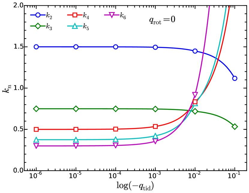
Figure 2: The effect of tidal perturbation strength on the tidal love numbers of a non-rotating Maclaurin spheroid up to order 6. The love numbers $k_{n}$ are degenerate with respect to $m$. The orbital radius is taken to be that of Tethys.

Figure 2 shows the calculated $k_{n}$ for the non-rotating Maclaurin spheroid as a function of $q_{\rm tid}$ up to order $n=6$, with $R/a$ taken to be that for Tethys and Saturn. For a small tidal perturbation, we find that $k_{n}$ approaches the analytical result of Eqn. (40). Conversely, as $q_{\rm rot}$ approaches unity from below, the love numbers diverge, with $k_{n}$ decreasing for $n\leq 3$ and increasing for $n>3$. The departure from the analytical solution becomes significant ($\left|\Delta k_{n}\right|>0.1$) for $-q_{\rm tid}>10^{-3}$, whereas for values representative of the largest Saturnian satellites, $k_{2}$ matches the analytic value to within our numerical precision.

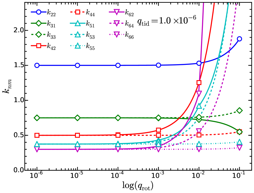
Figure 3: The effect of rotation rate on the tidal love numbers of Maclaurin spheroid up to order 6. The $k_{nm}$ for a given $n$ are found to split at high rotation rates. $q_{\rm tid}$ is kept constant at $1.0\times 10^{-6}$, and the orbital radius is taken to be that of Tethys.

In general, the tidal response of a gas giant planet will not be a perturbation to a perfect sphere, but to a spheroidal shape dominated by rotational flattening. Therefore, simulation of the tidal response in the absence of rotation is not generally applicable to real gas giants. When we simulate a Maclaurin spheroid with both finite $q_{\rm rot}$ and $q_{\rm tid}$, we find a different behavior for $k_{nm}$ as defined by Eqn. (41). Figure 3 shows the calculated $k_{nm}$ for a Maclaurin spheroid with a constant $q_{\rm tid}$ and a variable $q_{\rm rot}$. When the magnitude of $q_{\rm rot}$ is comparable to $q_{\rm tid}$, the tidal response matches the expected analytical result. However, for $q_{\rm rot}>10^{-3}$, we can see that the degeneracy of $k_{nm}$ with $m$ is broken, and all permitted $k_{nm}$ deviate from the expected values. In other words, Eqn. (42) becomes

$$\begin{cases}k_{nm}=0,&n\mathrm{~{}and~{}}m\mathrm{~{}opposite~{}parity}\\ k_{nm}\neq\mathrm{const},&n\mathrm{~{}and~{}}m\mathrm{~{}same~{}parity},\\ \end{cases}$$ (43)

and all permitted $k_{nm}$ deviate from the expected values. We also note that these deviations become pronounced earlier for the higher order $n$.

3.2 Two concentric Maclaurin Spheroids

Proceeding to more complicated interior structures has proved challenging for analytical or semi-analytical methods. Even the next simplest model with two constant-density layers does not have a closed form solution for arbitrary order $n$. Folonier et al. [4] present an extension of Clairaut theory for a multi-layer planet under the approximation that the level surfaces are perfect ellipsoids. Under this approximation, they derive an analytic solution for the distortion in response to a tidal perturbation only. This yields an expression for $k_{2}$ as a function of two ratios of properties of the two layers, $a_{1}/a$ and $\rho_{0}/\rho_{1}$. Table 1 shows a comparison of our calculated $k_{2}$ with the analytic result from Folonier et al. [4] for a selection of parameters spanning a range of $a_{1}/a$ and $\rho_{0}/\rho_{1}$. All of our results using the CMS method differ from those using Clairaut theory by less than $10^{-5}$. This provides an important test of the correctness of the interior potentials used in our approach. It also indicates that ellipsoids, while not exact, are a very good approximation for the degree 2 tidal response shape in the limit of very small $q_{\rm tid}$, and $q_{\rm rot}=0$.

3.3 Polytrope of index unity

The polytrope of index unity defines a more realistic barotrope that also lends itself to semi-analytic analyses. It corresponds to the relation

$$P=K\rho^{2}$$ (44)

where the polytropic constant $K$ can be chosen to match the planet’s physical parameters. For a nonrotating $n=1$ polytrope, the density distribution is given by

$$\rho=\rho_{c}\frac{\sin\pi\lambda}{\pi\lambda}$$ (45)

where $\rho_{c}$ is the density at the center of the planet. To obtain the first approximation of $\delta_{j}$, we differentiate Eqn. (45) by $\lambda$:

$$\frac{d(\rho/\rho_{c})}{d\lambda}=\frac{\cos\pi\lambda}{\lambda}-\frac{\sin\pi\lambda}{\pi\lambda^{2}}.$$ (46)

We then correct this profile to be consistent with the given $q_{\rm rot}$ via the method introduced in Section 2.5. Scaling the densities to maintain the total mass of the planet has a straightforward interpretation for a polytropic barotrope, as it is equivalent to changing $K$.

For the Maclaurin spheroid the lowest degree love number was

$$k_{2}=\frac{3}{2}.$$ (47)

Considering only the linear response to a purely rotational perturbation, we define a general degree 2 linear response parameter $\Lambda_{2}$ as

$$J_{2}=\Lambda_{2}q_{\rm rot}.$$ (48)

Whereas $\Lambda_{2}=1/2$ for the Maclaurin spheroid, for the polytrope of index unity the analytic result is [8]

$$\Lambda_{2}=\left(\frac{5}{\pi^{2}}-\frac{1}{3}\right).$$ (49)

Considering linear response only, one finds in general

$$k_{2}=3\Lambda_{2},$$ (50)

valid in the limit $q_{\rm rot}\ll 1$ and $q_{\rm tid}\ll 1$, for any barotrope in hydrostatic equilibrium. Thus, for the polytrope of index unity in this limit,

$$k_{2}=\frac{15}{\pi^{2}}-1=0.519817755.$$ (51)

We compare this to a CMS simulation of the $n=1$ polytrope model with 128 layers, $q_{\rm rot}=0$, $q_{\rm tid}=10^{-6}$, and Tethys’ $R/a$. The simulation results agree with the expected relation $J_{2}=2C_{22}$ to numerical precision, and yield $k_{2}=0.519775$. This provides a test of the multi-layer CMS approach subject to a tidal-only perturbation. The CMS result matches our Eqn. (51) benchmark to better than the precision with which we could measure this parameter using the Juno spacecraft. The small difference can be attributed to approximation of a continuous polytrope by 128 layers in the CMS simulation. Wisdom and Hubbard [24] (Eqn. 15) show the relative discretization error of a CMS polytrope model to be $\sim 10^{-3}$ for $N=128$, roughly consistent with our calculated difference.

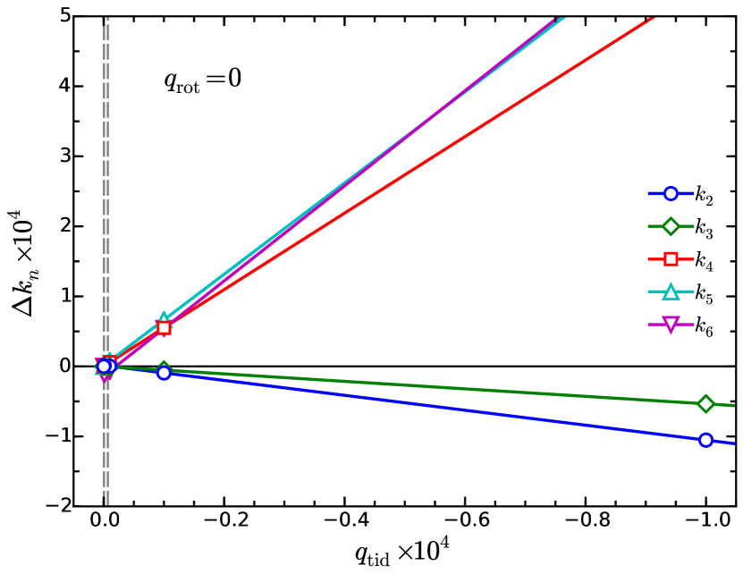
Figure 4: The effect of tidal perturbation strength on the tidal love numbers of a non-rotating planet with an $N=1$ polytrope equation of state, up to order 6. $\Delta k_{n}$ is the shift in love number $k_{n}$ from the limit of low $q{\rm tid}$. The love numbers $k_{n}$ are degenerate with respect to $m$. The orbital radius is taken to be that of Tethys. The vertical, dashed gray lines show $q_{\rm tid}$ for Tethys-Saturn and Io-Jupiter.

Similar to the calculations on the Maclaurin spheroid in Section 3.1, we performed additional $N=128$ polytrope simulations with finite $q_{\rm tid}$ and $q_{\rm rot}=0$. Once again, we find our calculated $k_{nm}$ to be degenerate with $m$ for the tidal-only simulations, in agreement with Eqn. (42). Figure 4 shows the behavior of $k_{n}$ for $n\leq 6$ for these tidal-only polytrope simulations. We only present these results up to $q_{\rm tid}\sim 10^{-4}$, because above that value effects of the triaxial shape on the pressure-density profile would require iterated relaxation to the polytropic relation, as discussed in Section 2.5. We observe that realistic values for $q_{\rm tid}$ have negligible effect on the tidal response. Even for the Io-Jupiter system, the effect of finite $q_{\rm tid}$ on $k_{nm}$ is near the numerical noise level. The general behavior is quite similar to the case of the single Maclaurin spheroid. For small tidal perturbations, the polytrope $k_{n}$ approach values smaller than the Maclaurin spheroid case, with $k_{2}$ asymptoting to the analytic limit in Eqn. (51). Similar to the Maclaurin spheroid, the behavior as $q_{\rm rot}$ increases from zero sees $k_{n}$ decrease for $n\leq 3$ and increase for $n>3$. The deviation from the low $q_{\rm tid}$ value is also less pronounced for the more realistic polytrope density distribution than for the Maclaurin spheroid. This is to be expected since there is less mass concentrated in the outer portion of the polytrope model.

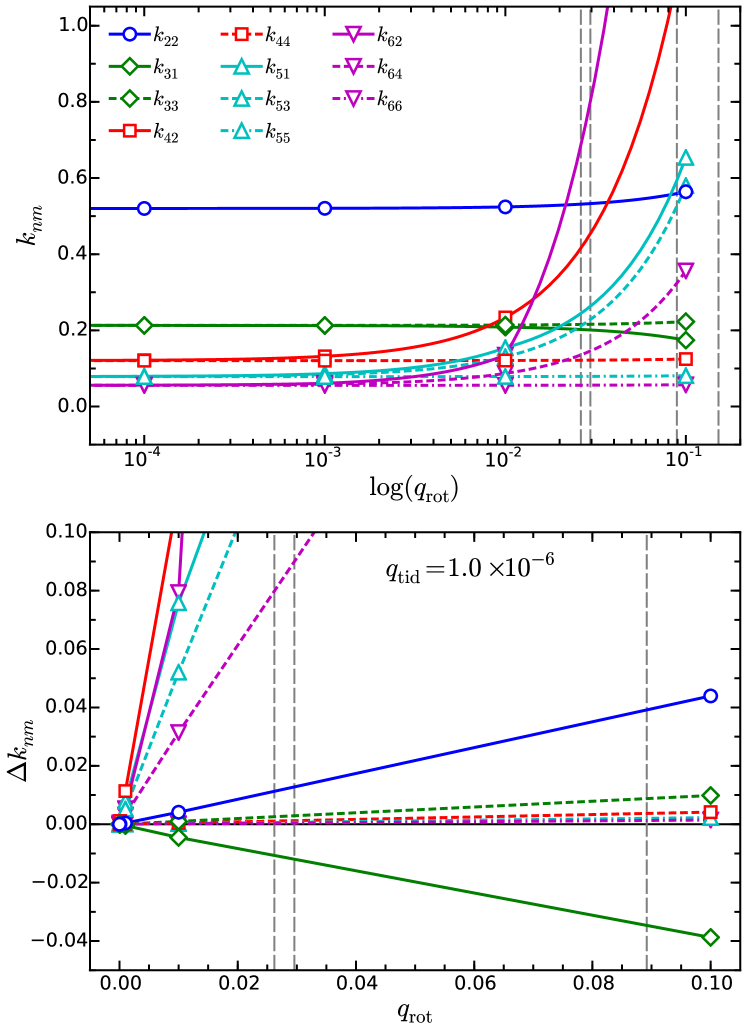
Figure 5: Top: The effect of rotation rate on the tidal love numbers of a planet with an $N=1$ polytrope equation of state, up to order 6. The $k_{nm}$ for a given $n$ are found to split at high rotation rates. $q_{\rm tid}$ is kept constant at $1.0\times 10^{-6}$, and the orbital radius is taken to be that of Tethys. The vertical, dashed gray lines show $q_{\rm rot}$ for Neptune, Uranus, Jupiter and Saturn. Bottom: Shift in $k_{nm}$ as a function of $q_{\rm rot}$ on a linear scale.

Figure 5 shows the effect of variable $q_{\rm rot}$ on polytrope models with constant $q_{\rm tid}$. Once again, we find that $k_{nm}$ degeneracy with respect to $m$ breaks, in agreement with Eqn. (43), as $q_{\rm rot}$ increases. Although the splitting of $k_{nm}$ is somewhat diminished from the single Maclaurin spheroid results, the deviations are still significant at large values of $q_{\rm rot}\sim 10^{-2}$ consistent with the rapidly-rotating gas giants. The shift in $k_{nm}$ shows a nearly linear increase in magnitude with increasing $q_{\rm rot}$, with potentially observable increases in $k_{2}$ for both the ice giant and gas giant planets. The general behavior of $k_{nm}$ is very similar between these tests with two very different density profiles. The relative magnitudes and directions of all $k_{nm}$ up to $n=6$ are similar between the two cases. This indicates that the effect should be ubiquitous in all fast-spinning liquid bodies, and relatively insensitive to the density profile of the planet.

4 Saturn’s tidal response

4.1 Saturn interior models

Lainey et al. [19] present the first determination of the love number $k_{2}$ for a gas giant planet using a dataset of astrometric observations of Saturn’s coorbital moons. Their observed value $k_{2}=0.390\pm 0.024$ is much larger than the theoretical prediction of 0.341 by Gavrilov and Zharkov [5]. Here we present calculations suggesting that the enhancement of Saturn’s $k_{2}$ is the result of the influence of the planet’s rapid rotation, rather than evidence for a nonstatic tidal response or some other breakdown of the hydrostatic theory.

For the purposes of this calculation, we use two relatively simple models for Saturn’s interior structure, fitted to physical parameters determined by the Voyager and Cassini spacecraft. Table The Concentric Maclaurin Spheroid method with tides and a rotational enhancement of Saturn’s tidal response summarizes the physical parameters used in our models. We fit our models to minimize the difference in zonal harmonics from those determined from Cassini [13]. We consider two different internal rotation rates based on magnetic field measurements from Voyager [3] and Cassini [6], which lead to two different values of $q_{\rm rot}$.

In principle, the tidal response of a heterogeneous body will also be different for satellites with different sizes and orbital parameters. To address this, we also consider the effect of two major satellites, Tethys and Dione, with different values for $q_{\rm tid}$ and $R/a$ [1]. These two satellites, along with their respective coorbital satellites, were used in the determination of $k_{2}$ by Lainey et al. [19].

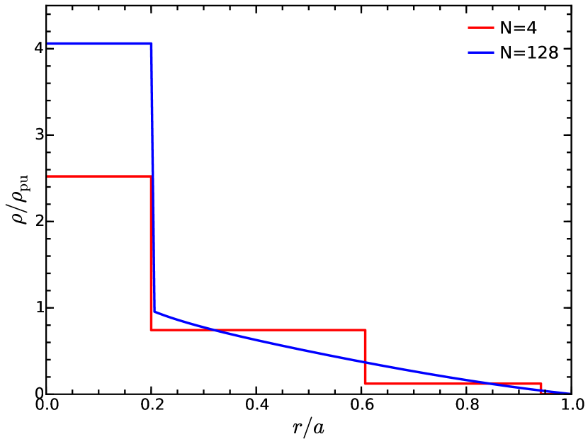
Figure 6: Density structure of simple Saturn models. The blue curve shows an $N=128$ model having a dense core within $r=0.2a$ and a polytropic outer envelope. The red curve shows an $N=4$ model with the same core constraints. Both models have densities adjusted to match $J_{2}$ measured by Cassini [Jacobson et al., 2006].

For the interior density profile, our first model assumes a constant-density core surrounded by a polytropic envelope following Eqn. (44). We constrain the radius of the core to be $a_{\rm core}/a=0.2$, leaving the mass $m_{\rm core}/M$ as a parameter which is adjusted to match the observed Saturn $J_{2}$. The fitted model using the Voyager rotation period matches both $J_{2}$ and $J_{4}$ to within the error bars, but with the Cassini rotation period it matches only $J_{2}$. In hydrostatic equilibrium, the two different rotation rates lead to differences in shape of equipotential surfaces and, therefore, also to different best fits to $m_{\rm core}/M$. The envelope polytrope is scaled in order to maintain $M$. Figure 6 shows the density profile of one such model. We consider a model with a total of 128 layers, for which the CMS model has a discretization error [24] smaller than uncertainty in the observations of Saturn’s $k_{2}$.

Our second model has only four spheroids ($N=4$), also depicted in Figure 6, with densities and radii adjusted to yield agreement with both observed $J_{2}$ and observed $J_{4}$ as given in Table The Concentric Maclaurin Spheroid method with tides and a rotational enhancement of Saturn’s tidal response.

These two simple models, while not particularly realistic, capture the major features of Saturn’s internal structure. It is well established that the details of Saturn’s internal structure are largely degenerate, with a wide range of possible core sizes and densities adequately matching the few observational constraints [18, 7, 21]. The qualitative similarities between our Maclaurin spheroid and polytrope simulations (Sections 3.1 and 3.3) indicate that the rotational enhancement of $k_{2}$ should be a robust prediction regardless of the particular details of the interior profile. A comparison between our polytrope plus core and four layer models provides another test of the sensitivity of $k_{2}$ to interior structure. We do not consider here the influence of differential rotation [9, 17, 2, 24], which might have an influence on the gravitational response in comparison to the solid-body rotation considered here. However, since the effect of realistic deep flow patterns on the low order zonal harmonics is small [2], we expect that they would cause negligible further changes in the rotational enhancement of $k_{2}$.

4.2 Calculated $k_{2}$ for Saturn

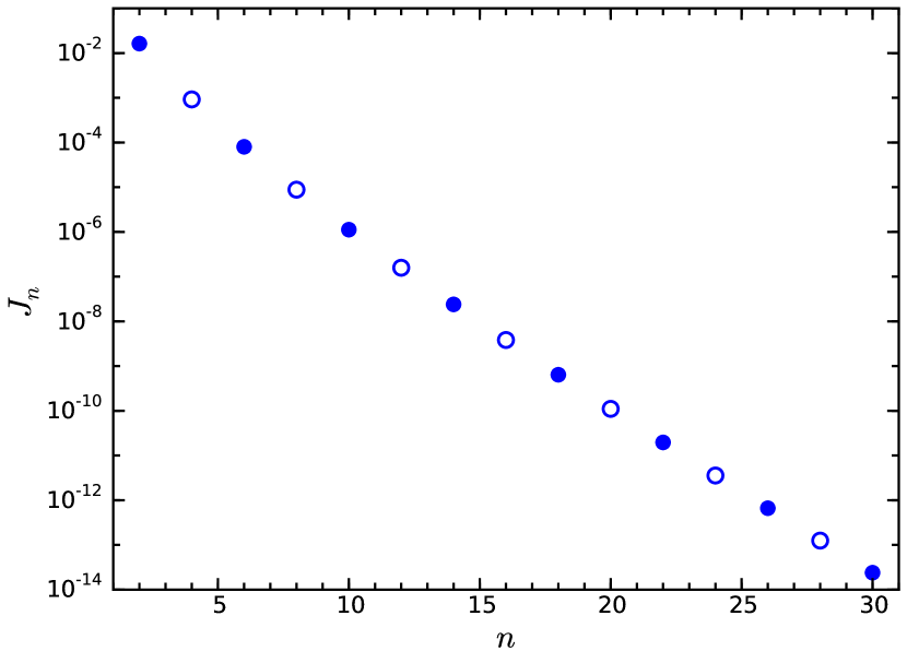
Figure 7: The zonal harmonics $J_{n}$ for the Cassini Saturn model. Positive values are shown as filled and negative as empty.

We take our baseline model to be the $N=128$ CMS core plus polytrope model with physical parameters fitted to Cassini observations. Figure 7 shows the calculated zonal harmonics $J_{n}$ up to order $n=30$. The even $J_{n}$ decrease smoothly in magnitude with increasing $n$, with the slope decreasing at higher $n$. $J_{n}$ is negative when $n$ is divisible by 4, and positive otherwise. The calculated $J_{n}$ are essentially indistinguishable from those calculated for the rotation only case with the same $q_{\rm rot}$, as is expected given $q_{\rm rot}\gg q_{\rm tid}$.

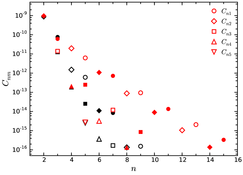
Figure 8: In red, the tesseral harmonics $C_{nm}$ for the Cassini Saturn model. In black, $C_{nm}$ for the same density profile and same value of $q_{\rm tid}$, but with $q_{\rm rot}=0$. Positive values are shown as filled and negative as empty.

Figure 8 shows the magnitude of $C_{nm}$ for the core plus polytrope model with Cassini rotation. Changing the number of layers, satellite parameters or the rotation rate to the Voyager value leads to a shift in the values, but the relative magnitudes and signs of $C_{nm}$ remain approximately the same. In the same figure, we also compare the $C_{nm}$ for a non-rotating planet having the same density profile $\rho(\lambda_{i})$. Here we see significant shifts in the magnitudes $C_{nm}$, although the signs remain the same. For the rotating model, $C_{nm}$ is similar for most points where $n=m$, but with magnitudes significantly larger when $m<n$. The only exception to this trend is $C_{31}$ which is lower for the rotating model. These results are all broadly consistent with the splitting of $k_{nm}$ observed for the polytrope in Section 3.3.

Table 3 summarizes our calculated values for $k_{2}$ for 5 different models. The identifying labels “Cassini” and “Voyager” use the observed rotation rate from Jacobson et al. [13], and Desch and Kaiser [3] respectively, while “non-rotating” is a model with $q_{\rm rot}=0$. The “non-rotating” model uses the same “Cassini” density profile, meaning that its density-pressure profile has not been relaxed to be in equilibrium for zero rotation. It does, however, allow us to quantify the effect of rotation on the tidal response by comparison with the “Cassini” model. “Tethys” and “Dione” refer to models with the satellite parameters $q_{\rm tid}$ and $R/a$ corresponding to those satellites, whereas “no tide” is an analogous model with finite $q_{\rm rot}$ only. “$N=128$” uses the polytrope outer envelope with constant density inner core, whereas “$N=4$” is the model which independently adjusts layer densities to match the observed $J_{2}$ and $J_{4}$.

Each of the rotating models yields a calculated $k_{2}$ value matching the observation of Lainey et al. [19] within their error bars. We find that the difference between the $k_{2}$ values associated with the satellites Tethys and Dione is $\sim$0.0003, well below the current sensitivity limit. Using the $\sim$2.5% higher “Voyager” rotation rate leads to a decrease of $\sim$0.01 in $k_{2}$.

In Table 3, we also show the calculated $J_{2}$, $J_{4}$ and $J_{6}$ following the convergence of the gravitational field in response to the tidal perturbation. For the core plus polytrope model, the rotation rate from Voyager is more consistent with the $J_{4}$ and $J_{6}$ from Jacobson et al. [13]. This doesn’t necessarily mean that the Voyager rotation rate is more correct, just that it allows a better fit for our simplified density model. Nonetheless, our fitted gravitational moments are much closer to each other than to those from the pre-Cassini model of Gavrilov and Zharkov [5].

In comparison to the other models, the outlier is the non-rotating model, which underestimates the $k_{2}$ by $\sim 9.4$% compared to a rotating body with the same density distribution. This calculated enhancement accounts for most of the difference between the observation of $k_{2}=0.390\pm.024$ [19] and the classical theory result of 0.341 [5]. We attribute our non-rotating model’s larger $k_{2}$ to our different interior model which matches more recent constraints on Saturn’s zonal gravitational moments $J_{2}$–$J_{6}$.

In addition to the difference in $k_{2}$, the non-rotating model also predicts slightly different tidal components of the zonal gravitational moments. Finding the difference in values between the “no tide” model and the analogous tidal model yields $J_{2,{\rm tid}}=1.7254\times 10^{-10}$, $J_{4,{\rm tid}}=-2.732\times 10^{-11}$ and $J_{6,{\rm tid}}=4.14\times 10^{-12}$, which are different than calculated zonal moments for the “non-rotating” model.

It may be initially surprising that the four-layer model yields a $k_{2}$ value only $\sim$0.0007 different than the polytrope model. The two models represent two very different density structures that lead to similar low-order zonal harmonics. The fact these two models are indistinguishable by their $k_{2}$ suggests that the tidal response of Saturn is only a weak function of the detailed density structure within the interior of the planet. This behavior can be understood by referring to Eqn. (50), which shows that to lowest order, $k_{2}$ and $\Lambda_{2}$ contain the same information about interior structure. This statement is not true when we include a nonlinear response to rotation and tides. Thus, future high-precision measurements of the $k_{nm}$ of jovian planets, say to better than $0.1\%$, will be useful for constraining basic parameters such as the interior rotation rate of the planet, and may help to break the current degeneracy of interior density profiles. The theory presented in this paper is intended to match the anticipated precision of such future measurements.

5 Summary

The CMS method for calculating a self-consistent shape and gravitational field of a static liquid planet has been extended to include the effect of a tidal potential from a satellite. This is expected to represent the largest contribution to the low-order tesseral harmonics measured by Juno and future spacecraft studies of the gas giants. This approach has been benchmarked against analytical results for the tidal response of the Maclaurin spheroid, two constant density layers, and the polytrope of index unity.

We highlight for the first time the importance of the high rotation rate on the tidal response of the gas giants. CMS simulations of the tidal response on bodies with large rotational flattening show significant deviation in the tesseral harmonics of the gravitational field as compared to simulations without rotation. This includes splitting of the love numbers into different $k_{nm}$ for any given order $n>2$. Meanwhile, it leads to an observable enhancement in $k_{2}$ compared to a non-rotating model.

This rotational enhancement of the $k_{2}$ love number for a simplified interior model of Saturn agrees with the recent observational result [19], which found $k_{2}$ to be much higher than previous predictions. Our predicted values of $k_{2}$ are robust for reasonable assumptions of interior structure, rotation rate and satellite parameters. The Juno spacecraft is expected to measure Jupiter’s gravitational field to sufficiently high precision to measure lower order tesseral components arising from Jupiter’s large moons, and we predict an analogous rotational enhancement of $k_{2}$ for Jupiter. Our high-precision tidal theory will be an important component of the search for non-hydrostatic terms in Jupiter’s external gravity field.

References

Table 1: Comparing two-layer models

$a_{1}/a$	$\rho_{0}/\rho_{1}$	$k_{2}$ CMS	$k_{2}$ Clairaut
0.1	0.5	1.496283	1.496286
0.3	0.5	1.411183	1.411185
0.5	0.1	0.465714	0.465716
0.5	0.3	0.947967	0.947969
0.5	0.5	1.205309	1.205311
0.5	0.7	1.360183	1.360186
0.5	0.9	1.461667	1.461669
0.7	0.5	1.057405	1.057407
0.9	0.5	1.217192	1.217194

Note. — Calculated $k_{2}$ for a two layer model with $q_{\rm tid}=10^{-6}$, $q_{\rm rot}=0$ and Tethy’s $R/a$, for chosen values of ratio of radii and densities of the two layers. Results closely match the approximation using Clairaut theory in Folonier et al. [2015], Eqn. 41.

Table 2: Saturn Model Parameters

	Cassini	Voyager
$GM$	$3.7931208\times 10^{7}$		${\rm(km^{3}/s^{2})}$
$a$	$6.0330\times 10^{4}$		${\rm(km)}$
$J_{2}\times 10^{6}$	$16290.71$
$J_{4}\times 10^{6}$	$-935.83$
$J_{6}\times 10^{6}$	$86.14$
$q_{\rm rot}$	$0.1516163$	$0.1553029$
$r_{\rm core}/a$	$0.2$
$m_{\rm core}/M$	$0.133146$	$0.140478$
	Tethys	Dione
$q_{\rm tid}$	$-2.791103\times 10^{-8}$	$-2.364582\times 10^{-8}$
$R/a$	$4.8892$	$6.2620$

References. — a. Jacobson et al. [2006], b. Giampieri et al. [2006], c. Desch and Kaiser [1981], d. Archinal et al. [2011]

Note. — Identical parameters for Saturn are used with the exception of $q_{\rm rot}$, for which the rotation rate from both Cassini and Voyager are considered. A constant core density is fitted to match $J_{2}$, $J_{4}$, and $J_{6}$ for a converged figure.

Table 3: Calculated Saturn tidal responses

model		gravitational moment		normalized moment
Cassini	$J_{2}$	$1.62907100025\times 10^{-2}$	$J_{2}/q_{\rm rot}$	$0.10744694879478$
no tide	$J_{4}$	$-9.2027941201\times 10^{-4}$	$J_{4}/q_{\rm rot}$	$-0.606979160784\times 10^{-2}$
$N=128$	$J_{6}$	$8.014294995\times 10^{-5}$	$J_{6}/q_{\rm rot}$	$0.5285905549\times 10^{-3}$
non-rotating	$C_{22}$	$8.5288\times 10^{-10}$	$k_{2}$	$0.36669$
Tethys	$J_{2}$	$1.70576\times 10^{-9}$	$J_{2}/q_{\rm rot}$
$N=128$	$J_{4}$	$-1.351\times 10^{-11}$	$J_{4}/q_{\rm rot}$
	$J_{6}$	$2.2\times 10^{-13}$	$J_{6}/q_{\rm rot}$
Cassini	$C_{22}$	$9.6070\times 10^{-10}$	$k_{2}$	$0.41304$
Tethys	$J_{2}$	$1.629071017501\times 10^{-2}$	$J_{2}/q_{\rm rot}$	$0.1074469499328$
$N=128$	$J_{4}$	$-9.2027943932\times 10^{-4}$	$J_{4}/q_{\rm rot}$	$-0.60697917880\times 10^{-2}$
	$J_{6}$	$8.01429541\times 10^{-5}$	$J_{6}/q_{\rm rot}$	$0.5285905822\times 10^{-3}$
Voyager	$C_{22}$	$9.4136\times 10^{-10}$	$k_{2}$	$0.40473$
Tethys	$J_{2}$	$1.629071048760\times 10^{-2}$	$J_{2}/q_{\rm rot}$	$0.1048963407747$
$N=128$	$J_{4}$	$-9.3570887868\times 10^{-4}$	$J_{4}/q_{\rm rot}$	$-0.60250556585\times 10^{-2}$
	$J_{6}$	$8.30176108\times 10^{-5}$	$J_{6}/q_{\rm rot}$	$0.534552720\times 10^{-3}$
Cassini	$C_{22}$	$8.1325\times 10^{-10}$	$k_{2}$	$0.41272$
Dione	$J_{2}$	$1.629071019035\times 10^{-2}$	$J_{2}/q_{\rm rot}$	$0.1074469500340$
$N=128$	$J_{4}$	$-9.2027943688\times 10^{-4}$	$J_{4}/q_{\rm rot}$	$-0.60697917719\times 10^{-2}$
	$J_{6}$	$8.01429534\times 10^{-5}$	$J_{6}/q_{\rm rot}$	$0.528590578\times 10^{-3}$
Cassini	$C_{22}$	$9.6219\times 10^{-10}$	$k_{2}$	$0.41368$
Tethys	$J_{2}$	$1.629071019560\times 10^{-2}$	$J_{2}/q_{\rm rot}$	$0.1074469500686$
$N=4$	$J_{4}$	$-9.3583002600\times 10^{-4}$	$J_{4}/q_{\rm rot}$	$-0.61723571821\times 10^{-2}$
	$J_{6}$	$8.61400043\times 10^{-5}$	$J_{6}/q_{\rm rot}$	$0.568144705\times 10^{-3}$

References

- Archinal et al. [2011] Archinal, B.A., A’Hearn, M.F., Bowell, E., Conrad, A., Consolmagno, G.J., Courtin, R., Fukushima, T., Hestroffer, D., Hilton, J.L., Krasinsky, G.A., Neumann, G., Oberst, J., Seidelmann, P.K., Stooke, P., Tholen, D.J., Thomas, P.C., Williams, I.P., 2011. Report of the IAU Working Group on Cartographic Coordinates and Rotational Elements: 2009. Celest. Mech. Dyn. Astron. 109, 101–135. doi:10.1007/s10569-010-9320-4.
- Cao and Stevenson [2015] Cao, H., Stevenson, D.J., 2015. Gravity and Zonal Flows of Giant Planets: From the Euler Equation to the Thermal Wind Equation , 1–9URL: http://arxiv.org/abs/1508.02764, arXiv:1508.02764.
- Desch and Kaiser [1981] Desch, M.D., Kaiser, M.L., 1981. Voyager measurement of the rotation period of Saturn’s magnetic field. Geophys. Res. Lett. 8, 253--256. doi:10.1029/GL008i003p00253.
- Folonier et al. [2015] Folonier, H., Ferraz-Mello, S., Kholshevnikov, K.V., 2015. The flattenings of the layers of rotating planets and satellites deformed by a tidal potential. Celest. Mech. Dyn. Astron. 122, 183--198. URL: http://arxiv.org/abs/1503.08051, doi:10.1007/s10569-015-9615-6, arXiv:1503.08051.
- Gavrilov and Zharkov [1977] Gavrilov, S.V., Zharkov, V.N., 1977. Love numbers of the giant planets. Icarus 32, 443--449. URL: http://linkinghub.elsevier.com/retrieve/pii/001910357790015X, doi:10.1016/0019-1035(77)90015-X.
- Giampieri et al. [2006] Giampieri, G., Dougherty, M.K., Smith, E.J., Russell, C.T., 2006. A regular period for Saturn’s magnetic field that may track its internal rotation. Nature 441, 62--64. doi:10.1038/nature04750.
- Helled and Guillot [2013] Helled, R., Guillot, T., 2013. Interior Models of Saturn: Including the Uncertainties in Shape and Rotation. Astrophys. J. 767, 113. URL: http://stacks.iop.org/0004-637X/767/i=2/a=113?key=crossref.045d858be83734acdc0600277a318377, doi:10.1088/0004-637X/767/2/113.
- Hubbard [1975] Hubbard, W., 1975. Gravitational field of a rotating planet with a polytropic index of unity. Sov. Astron. 18, 621--624.
- Hubbard [1982] Hubbard, W., 1982. Effects of differential rotation on the gravitational figures of Jupiter and Saturn. Icarus 52, 509--515. URL: http://linkinghub.elsevier.com/retrieve/pii/0019103582900112, doi:10.1016/0019-1035(82)90011-2.
- Hubbard et al. [2014] Hubbard, W., Schubert, G., Kong, D., Zhang, K., 2014. On the convergence of the theory of figures. Icarus 242, 138--141. URL: http://linkinghub.elsevier.com/retrieve/pii/S001910351400428X, doi:10.1016/j.icarus.2014.08.014.
- Hubbard [2012] Hubbard, W.B., 2012. High-Precision Maclaurin-Based Models of Rotating Liquid Planets. Astrophys. J. 756, L15. URL: http://stacks.iop.org/2041-8205/756/i=1/a=L15?key=crossref.34b95153bc3fdfb844cab51abbdf75d3, doi:10.1088/2041-8205/756/1/L15.
- Hubbard [2013] Hubbard, W.B., 2013. Concentric Maclaurin Spheroid Models of Rotating Liquid Planets. Astrophys. J. 768, 43. URL: http://stacks.iop.org/0004-637X/768/i=1/a=43?key=crossref.a31bd47c857111e805198695ba70780e, doi:10.1088/0004-637X/768/1/43.
- Jacobson et al. [2006] Jacobson, R.A., Antresian, P.G., Bordi, J.J., Criddle, K.E., Ionasescu, R., Jones, J.B., Mackenzie, R.a., Meek, M.C., Parcher, D., Pelletier, F.J., Owen, W.M., Roth, D.C., Roundhill, I.M., Stauch, J.R., 2006. The gravity field of the Saturnian system from staellites observations and spacecraft tracking data. Astrophys. J. 132, 2520--2526. doi:10.1086/508812.
- Jeans [2009] Jeans, J.H., 2009. Problems of Cosmology and Stellar Dynamics. Cambridge University Press. URL: http://dx.doi.org/10.1017/CBO9780511694417.
- Kaspi [2013] Kaspi, Y., 2013. Inferring the depth of the zonal jets on Jupiter and Saturn from odd gravity harmonics. Geophys. Res. Lett. 40, 676--680. doi:10.1029/2012GL053873.
- Kaspi et al. [2010] Kaspi, Y., Hubbard, W.B., Showman, A.P., Flierl, G.R., 2010. Gravitational signature of Jupiter’s internal dynamics. Geophys. Res. Lett. 37, L01204. URL: http://doi.wiley.com/10.1029/2012GL053873, doi:10.1029/2009GL041385.
- Kong et al. [2013] Kong, D., Liao, X., Zhang, K., Schubert, G., 2013. Gravitational signature of rotationally distorted Jupiter caused by deep zonal winds. Icarus 226, 1425--1430. URL: http://linkinghub.elsevier.com/retrieve/pii/S0019103513003540, doi:10.1016/j.icarus.2013.08.016.
- Kramm et al. [2011] Kramm, U., Nettelmann, N., Redmer, R., Stevenson, D.J., 2011. Astrophysics On the degeneracy of the tidal Love number in multi-layer planetary models : application to Saturn and GJ 436b. Astron. Astrophys. 18, 1--7. doi:10.1051/0004-6361/201015803, arXiv:1101.0997.
- Lainey et al. [2016] Lainey, V., Jacobson, R.A., Tajeddine, R., Cooper, N.J., Robert, V., Tobie, G., Guillot, T., Mathis, S., 2016. New constraints on Saturn’s interior from Cassini astrometric data URL: http://arxiv.org/abs/1510.05870, arXiv:1510.05870.
- Munk and MacDonald [2009] Munk, W.H., MacDonald, G.J.F., 2009. The Rotation of the Earth: A Geophysical Discussion. Cambridge Monographs on Mechanics, Cambridge University Press. URL: https://books.google.com/books?id=klDqPAAACAAJ.
- Nettelmann et al. [2013] Nettelmann, N., Püstow, R., Redmer, R., 2013. Saturn layered structure and homogeneous evolution models with different EOSs. Icarus 225, 548--557. URL: http://linkinghub.elsevier.com/retrieve/pii/S0019103513001784, doi:10.1016/j.icarus.2013.04.018, arXiv:1304.4707.
- Tassoul [2015] Tassoul, J.L., 2015. Theory of Rotating Stars. (PSA-1). Princeton Series in Astrophysics, Princeton University Press. URL: https://books.google.com/books?id=nnJ9BgAAQBAJ.
- Wisdom [1996] Wisdom, J., 1996. Non-perturbative Hydrostatic Equilibrium URL: http://web.mit.edu/wisdom/www/interior.pdf.
- Wisdom and Hubbard [2016] Wisdom, J., Hubbard, W.B., 2016. Differential rotation in Jupiter: A comparison of methods. Icarus 267, 315--322. URL: http://dx.doi.org/10.1016/j.icarus.2015.12.030, doi:10.1016/j.icarus.2015.12.030.
- Zharkov and Trubitsyn [1978] Zharkov, V.N., Trubitsyn, V.P., 1978. The physics of planetary interiors. Parchart, Tucson, AZ.