Sparse Estimation of Multivariate
Poisson Log-Normal Models from Count Data

Abstract

Modeling data with multivariate count responses is a challenging problem due to the discrete nature of the responses. Existing methods for univariate count responses cannot be easily extended to the multivariate case since the dependency among multiple responses needs to be properly accommodated. In this paper, we propose a multivariate Poisson log-normal regression model for multivariate data with count responses. By simultaneously estimating the regression coefficients and inverse covariance matrix over the latent variables with an efficient Monte Carlo EM algorithm, the proposed regression model takes advantages of association among multiple count responses to improve the model prediction performance. Simulation studies and applications to real world data are conducted to systematically evaluate the performance of the proposed method in comparison with conventional methods.

1 Introduction

In this decade of data science, multivariate response observations are routine in numerous disciplines. To model such datasets, multivariate regression and multi-task learning models are common techniques to study and investigate the relationships between $q\geq 2$ responses and $p$ predictors. The former class of methods, e.g. [25, 23, 22] and [27], estimates the $p\times q$ regression coefficients as well as recover the correlation structures among response variables using regularization. The latter class of methods focuses on learning the shared features [13, 15, 14, 18] or common underlying structure(s) among multiple tasks [2, 20, 6, 31, 3] using regression approaches and enforcing regularization controls over the coefficient matrix. However, all such multivariate regression or multi-task learning models discussed above deal with continuous responses, none of them handle count data.

When responses are count variables, the Poisson model is a natural approach to model them, e.g., in domains such as influenza case count modeling [28], traffic accident analysis [24, 8] and consumer services [26]. However, Poisson regression models proposed in these works are either univariate or inferred via Bayesian approaches and no sparsity or feature selection is typically enforced over the coefficients. When count responses are multivariate, it is challenging to quantify the association among them due to the discrete nature of the data. One important approach is to model each dimension of count variables as the sum of independent Poisson variables with some common Poisson variables capturing dependencies [19]. A drawback of this method is that it can only model positive correlations. Recent literature [30, 16] models multivariate count data with novel Poisson graphical models which can handle both positive and negative dependencies. However, these works do not consider multivariate count data in the context of regression.

To consider a joint model for data with multivariate count responses, it is important to properly exploit the hidden associations among the count responses. One way to consider the joint model of multivariate count responses is via penalty-based model selection from the perspective of parameter regularization. The key idea is to allow the count responses to be independent of each other, while the regression coefficients are required to obey a certain common sparse structure. Hence the joint modeling is enabled because of the joint estimation of regression coefficients through appropriate penalties. Such a modeling strategy leads to an explicit loss function with tractable computational characteristics. However, this method overlooks the essential correlation among multiple count responses, which could result in poor prediction performance. There are also several recent papers that develop models of multivariate count data from the lens of conditional dependency. But these method typically are restricted to approximated likelihood functions under the framework of generalized liner models.

In this work, we propose a novel multivariate Poisson log-normal model for data with multiple count responses. The motivation to adopt the log-normal model is to borrow strength from regression under the multivariate normal assumption, which can simultaneously estimate regression coefficients and covariance structure. For the proposed model, the logarithm of the Poisson rate parameters is modeled as multivariate normal with a sparse inverse covariance matrix, which combines the strengths of sparse regression and graphical modeling to improve prediction performance. Thus, this approach can fully exploit the conditional dependency among multiple count responses. Estimating such model is non-trivial since it is intractable to derive an explicit analytical solution. Thus, to facilitate the estimation of model parameters, we develop an Monte Carlo EM algorithm which allows to iteratively estimate the regression coefficients using the Lasso penalty and the inverse covariance matrix by a graphical Lasso approach. By applying the proposed model to synthetic data and a real world influenza-like illness dataset, we demonstrate the effectiveness of the proposed method when modeling multivariate data with count responses.

It is worth pointing out that the proposed method is not restricted to adopt the Lasso penalty for regression parameters. It can be easily extended to other penalties such as the adaptive Lasso, group Lasso or fused Lasso. While covariance matrix estimation and inverse covariance matrix estimation have attracted significant attention in the literature [11, 25, 23], here we use this idea in the context of a multivariate regression for count data. Thus inverse covariance matrix estimation is conducted here to improve prediction performance, not just as an unsupervised procedure. One may call such a strategy supervised covariance estimation, which has not been widely studied in the literature. One exception is the multivariate regression for continuous responses [25, 29]. Therefore, to the best of our knowledge, our proposed method is a first to incorporate covariance matrix estimation into a multivariate regression model of count responses.

2 Multivariate Poisson Log-Normal model

In this section, we formally specify the Multivariate Poisson Log-Normal (MVPLN) model, and propose a Monte Carlo Expectation-Maximization (MCEM) algorithm for parameter estimation in detail.

2.1 The proposed model

Consider the multivariate random variable $\boldsymbol{\mathcal{Y}}=\{\mathcal{Y}^{(1)},$ $\mathcal{Y}^{(2)},\ldots,\mathcal{Y}^{(q)}\}^{T}\in\mathcal{Z}^{q}_{+}$, where the superscript $T$ denotes the transpose, and $\mathcal{Z}_{+}$ represents the set of all positive integers. For count data, it is reasonable to make the assumption that $\boldsymbol{\mathcal{Y}}$ follows the multivariate Poisson distribution. Without loss of generality, let’s assume that each dimension of $\boldsymbol{\mathcal{Y}}$, say $\mathcal{Y}^{(i)}$, follows the univariate Poisson distribution with parameter $\theta^{(i)}$, and is conditional independent of other dimensions given $\theta^{(i)}$. That is:

$$\mathcal{Y}^{(i)}\sim\mathit{Poisson}\left(\theta^{(i)}\right),~{}\theta^{(i)}\in\mathcal{R}_{+},~{}\forall i=1,2,\ldots,q$$ (1)

Let $\boldsymbol{x}={\{x^{(1)},x^{(2)},\ldots,x^{(p)}\}}^{T}\in\mathcal{R}^{p}$ denote the predictor vector. In order to establish relationship between $\boldsymbol{\mathcal{Y}}$ and $\boldsymbol{x}$, we consider the following regression model:

$$\boldsymbol{\theta}= \exp\left(\boldsymbol{B}^{T}\boldsymbol{x}+\boldsymbol{\varepsilon}\right)$$ (2)

$$\boldsymbol{\varepsilon}\sim N(0,\boldsymbol{\Sigma})$$

where $\boldsymbol{B}$ is a $p\times q$ coefficient matrix, and $\boldsymbol{\Sigma}$ is the $q\times q$ covariance matrix which captures the covariance structure of variable $\boldsymbol{\theta}={\{\theta^{(1)},\theta^{(2)},\ldots,\theta^{(q)}\}}^{T}$ given $\boldsymbol{x}$. Through the variable $\boldsymbol{\theta}$, we model the covariance structure of the count variable $\boldsymbol{\mathcal{Y}}$ indirectly. Fig. 1 shows the plate notation of the proposed MVPLN model.

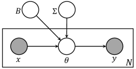
Figure 1: The plate notation of the proposed MVPLN model.

Given $n$ observations of the predictor $\boldsymbol{X}=[\boldsymbol{x}_{1},\boldsymbol{x}_{2},$ ${\ldots,\boldsymbol{x}_{n}]}^{T}$ and corresponding responses $\boldsymbol{Y}=[\boldsymbol{y}_{1},\boldsymbol{y}_{2},$ ${\ldots,\boldsymbol{y}_{n}]}^{T}$, the log-likelihood of the MVPLN model is:

$$\mathcal{L}(\boldsymbol{B},\boldsymbol{\Sigma})=\sum_{j=1}^{n}\log p(\boldsymbol{\mathcal{Y}}=\boldsymbol{y}_{j}\mid\boldsymbol{x}_{j}),$$ (3)

where

$$p(\boldsymbol{\mathcal{Y}}=\boldsymbol{y}\mid\boldsymbol{x})=\int_{\boldsymbol{\theta}}p(\boldsymbol{\mathcal{Y}}=\boldsymbol{y},\boldsymbol{\theta}\mid\boldsymbol{x})d\boldsymbol{\theta}=\int_{\boldsymbol{\theta}}p(\boldsymbol{\mathcal{Y}}=\boldsymbol{y}\mid\boldsymbol{\theta})p(\boldsymbol{\theta}\mid\boldsymbol{x})d\boldsymbol{\theta}$$ (4)

Here, $p(\boldsymbol{\mathcal{Y}}=\boldsymbol{y}\mid\boldsymbol{\theta})$ and $p(\boldsymbol{\theta}\mid\boldsymbol{x})$ follow multivariate Poisson distribution and multivariate log-normal distribution as derived in Section A of Supplementary Material, respectively. To jointly infer the sparse estimations of coefficient matrix $\boldsymbol{B}$ and covariance matrix $\boldsymbol{\Sigma}$, we adopt the regularized negative log-likelihood function with $l_{1}$ penalties as our loss function. To be specific, the loss function could be written as:

$$\mathcal{L}_{p}(\boldsymbol{B},\boldsymbol{\Sigma})=-\mathcal{L}(\boldsymbol{B},\boldsymbol{\Sigma})+\lambda_{1}||\boldsymbol{B}||_{1}+\lambda_{2}||\boldsymbol{\Sigma}^{-1}||_{1},$$ (5)

where $||\cdot||_{1}$ denote the $l_{1}$ matrix norm, and $\lambda_{1}>0,\lambda_{2}>0$ are two tuning parameters.

For convenience, we use the following notation to present the proposed MVPLN model in the rest of the paper. Normal lower case letters, e.g. $x$ and $y$, represent scalars. While, bold lower case letters, e.g. $\boldsymbol{x}$ and $\boldsymbol{y}$, are used to represent column vectors, and bold upper case letters in the calligraphic font, e.g. $\boldsymbol{\mathcal{X}}$ and $\boldsymbol{\mathcal{Y}}$, denote random column vectors. Let letters with superscript in parentheses, e.g. $x^{(i)}$, denote the $i^{th}$ component of the corresponding vector $\boldsymbol{x}$. Matrices are represented by bold upper case letters in normal font, e.g. $\boldsymbol{X}$ and $\boldsymbol{Y}$. Letters in lower case with two subscripts, e.g. $x_{i,j}$, denote the $(i,j)$ entry of the corresponding matrix $\boldsymbol{X}$.

2.2 Monte Carlo EM algorithm for parameter estimation

In order to obtain the estimations of MVPLN model parameters $\boldsymbol{B}$ and $\boldsymbol{\Sigma}$, we could simply solve the following optimization problem:

$$\hat{\boldsymbol{B}},\hat{\boldsymbol{\Sigma}}=\operatornamewithlimits{argmin}_{\boldsymbol{B},\boldsymbol{\Sigma}}\mathcal{L}_{p}(\boldsymbol{B},\boldsymbol{\Sigma}).$$ (6)

However, it’s difficult to directly minimize the objective function defined above due to the complicated integral in Equation (4). Thus, we turn to an iterative approach for the solution. We treat $\boldsymbol{\theta}$ as latent random variables, and apply the EM algorithm to obtain the maximum likelihood parameter estimation (MLE). However, we cannot derive the analytical form of the expected log-likelihood of the model due to the integral in Equation (4). Here, we adopt a Monte Carlo variant of the EM algorithm for an approximate solution.

2.2.1 Monte Carlo (MC) E-step

In the MC E-step of iteration $t+1$, instead of trying to derive the close form of the conditional probability distribution of $\boldsymbol{\theta}_{j}$, we draw $m$ random samples of $\boldsymbol{\theta}_{j}$, say $\boldsymbol{\Theta}_{j}={\left[\boldsymbol{\theta}_{j}^{(1)},\boldsymbol{\theta}_{j}^{(2)},\ldots,\boldsymbol{\theta}_{j}^{(m)}\right]}^{T}$, from $p(\boldsymbol{\theta}_{j}\mid\boldsymbol{\mathcal{Y}}=\boldsymbol{y}_{j},\boldsymbol{x}_{j};\boldsymbol{B}^{(t)},\boldsymbol{\Sigma}^{(t)})$, and approximate the expected log-likelihood function with:

$$\tilde{Q}(\boldsymbol{B}, \boldsymbol{\Sigma}\mid\boldsymbol{B}^{(t)},\boldsymbol{\Sigma}^{(t)})=\sum_{j=1}^{n}\frac{1}{m}\sum_{\tau=1}^{m}\log p(\boldsymbol{\mathcal{Y}}=\boldsymbol{y}_{j},\boldsymbol{\theta}_{j}^{(\tau)}\mid\boldsymbol{x}_{j};\boldsymbol{B}^{(t)},\boldsymbol{\Sigma}^{(t)}).$$ (7)

Drawing random samples of $\boldsymbol{\theta}_{j}$ can be achieved with the Metropolis Hasting algorithm. In order to reduce the burn-in period of the Metropolis Hasting algorithm, we adopt the tailored normal distribution [7] as our proposal distribution. Since $p(\boldsymbol{\theta}_{j}\mid\boldsymbol{\mathcal{Y}}=\boldsymbol{y}_{j},\boldsymbol{x}_{j};\boldsymbol{B}^{(t)},\boldsymbol{\Sigma}^{(t)})\propto p(\boldsymbol{\mathcal{Y}}=\boldsymbol{y}_{j},\boldsymbol{\theta}_{j}\mid\boldsymbol{x}_{j};\boldsymbol{B}^{(t)},\boldsymbol{\Sigma}^{(t)})$, if we let $f(\boldsymbol{\theta}_{j})=p(\boldsymbol{\mathcal{Y}}=\boldsymbol{y}_{j},\boldsymbol{\theta}_{j}\mid\boldsymbol{x}_{j};\boldsymbol{B}^{(t)},\boldsymbol{\Sigma}^{(t)})$, the initial value $\boldsymbol{\theta}_{j}^{(0)}$ of the location parameter for the tailored normal distribution should be the mode of $f(\boldsymbol{\theta}_{j})$, and the covariance matrix is $\tau{(-\boldsymbol{H}(\boldsymbol{\theta}_{j}^{(0)}))}^{-1}$, where $\boldsymbol{H}(\boldsymbol{\theta}_{j}^{(0)})$ denotes the Hessian matrix of $\log f(\boldsymbol{\theta}_{j})$ at $\boldsymbol{\theta}_{j}^{(0)}$, and $\tau$ is a tuning parameter. Considering the performance issue, we adopt a linear approximation approach with the first order Taylor expansion to solve $\boldsymbol{\theta}_{j}^{(0)}$. In this case, the approximate analytical solution of $\boldsymbol{\theta}_{j}^{(0)}$ is $\boldsymbol{\theta}_{j}^{(0)}=\boldsymbol{e}^{\boldsymbol{\kappa}_{j}}$ where

$$\boldsymbol{\kappa}_{j}= {\left(\operatorname{diag}\left(\boldsymbol{e}^{\boldsymbol{\kappa}_{j}^{(0)}}\right)+{\boldsymbol{\Sigma}^{(t)}}^{-1}\right)}^{-1}\Big{(}\boldsymbol{y}_{j}-\boldsymbol{1}+{\boldsymbol{\Sigma}^{(t)}}^{-1}{\boldsymbol{B}^{(t)}}^{T}\boldsymbol{x}_{j}+\operatorname{diag}\left(\boldsymbol{e}^{\boldsymbol{\kappa}_{j}^{(0)}}\right)\boldsymbol{\kappa}_{j}^{(0)}-\boldsymbol{e}^{\boldsymbol{\kappa}_{j}^{(0)}}\Big{)}.$$

Here, $\boldsymbol{\kappa}_{j}^{(0)}=\log\boldsymbol{y}_{j}$. In the case that the covariance matrix $\tau{(-\boldsymbol{H}(\boldsymbol{\theta}_{j}^{(0)}))}^{-1}$ is not positive semidefinite, the nearest positive semidefinite matrix to $\tau{(-\boldsymbol{H}(\boldsymbol{\theta}_{j}^{(0)}))}^{-1}$ is used to replace $\tau{(-\boldsymbol{H}(\boldsymbol{\theta}_{j}^{(0)}))}^{-1}$ [17]. The details for Metropolis Hasting algorithm and the derivation of the tailored normal distribution as the proposal distribution are provided in Section B of the Supplementary Material.

2.2.2 M-step: maximize approximate penalized expected log-likelihood

If we let $\boldsymbol{\Omega}=\boldsymbol{\Sigma}^{-1}$ and $\boldsymbol{\varphi}_{\tau,j}=(\log\boldsymbol{\theta}_{j}^{(\tau)}-\boldsymbol{B}^{T}\boldsymbol{x}_{j})$, with the Monte Carlo approximation of the expected log-likelihood in the MC E-step, the optimization problem we need to solve in the M-step of the MCEM algorithm can be reformulated as:

$$\boldsymbol{B}^{(t+1)},\boldsymbol{\Sigma}^{(t+1)}= \operatornamewithlimits{argmin}_{\boldsymbol{B},\boldsymbol{\Omega}}\bigg{\{}\frac{1}{mn}\operatorname{tr}\left(\boldsymbol{\Phi}^{T}\boldsymbol{\Phi}\boldsymbol{\Omega}\right)-\log|\boldsymbol{\Omega}|+\lambda_{1}||\boldsymbol{B}||_{1}+\lambda_{2}||\boldsymbol{\Omega}||_{1}\bigg{\}}$$ (8)

where $\boldsymbol{\Phi}={[\boldsymbol{\varphi}_{1,1},\boldsymbol{\varphi}_{2,1},\ldots,\boldsymbol{\varphi}_{m,1},\boldsymbol{\varphi}_{1,2},\boldsymbol{\varphi}_{2,2},\ldots,\boldsymbol{\varphi}_{m,2},\ldots,\boldsymbol{\varphi}_{m,n}]}^{T}$. The optimization problem defined in Equation (8) is not convex. However, it is convex w.r.t. either $\boldsymbol{B}$ or $\boldsymbol{\Omega}$ with the other fixed [25]. Thus, we present an iterative algorithm that optimizes the objective function in Equation (8) alternatively w.r.t. $\boldsymbol{B}$ and $\boldsymbol{\Omega}$.

With $\boldsymbol{B}$ fixed at $\boldsymbol{B}_{0}$, the optimization problem in Equation (8) yields:

$$\boldsymbol{\Omega}(\boldsymbol{B}_{0})=\operatornamewithlimits{argmin}_{\boldsymbol{\Omega}}\bigg{\{} \frac{1}{mn}\operatorname{tr}\left(\boldsymbol{\Phi}^{T}\boldsymbol{\Phi}\boldsymbol{\Omega}\right)-\log|\boldsymbol{\Omega}|+\lambda_{2}||\boldsymbol{\Omega}||_{1}\bigg{\}},$$ (9)

which is the similar problem studied in [11]. We solve this problem with the graphical lasso approach.

When $\boldsymbol{\Omega}$ is fixed at $\boldsymbol{\Omega}_{0}$, we have the following optimization problem:

$$\boldsymbol{B}(\boldsymbol{\Omega}_{0})=\operatornamewithlimits{argmin}_{\boldsymbol{B}}\bigg{\{}\frac{1}{mn}\operatorname{tr}\left(\boldsymbol{\Phi}^{T}\boldsymbol{\Phi}\boldsymbol{\Omega}_{0}\right)+\lambda_{1}||\boldsymbol{B}||_{1}\bigg{\}},$$ (10)

which is similar to the problem solved by Lasso, and we could adopt the cyclical coordinate descent algorithm [10] to obtain the estimation of $\boldsymbol{B}$. However, considering the computational burden already brought in by the MCMC approximation in the MC E-step, we solve the optimization problem in Equation (10) approximately where the $l_{1}$ matrix norm $||\boldsymbol{B}||_{1}$ is replaced by its quadratic approximation $\operatorname{tr}({\boldsymbol{B}^{\prime}}^{T}\boldsymbol{B}^{\prime})$ where $\boldsymbol{B}^{\prime}=\boldsymbol{B}\circ({1}/{\sqrt{|\hat{\boldsymbol{B}}|}})$. Here, $\circ$ denotes the Hadamard (element-wise) product, $\hat{\boldsymbol{B}}$ denotes the current estimation of $\boldsymbol{B}$, and $1/\sqrt{|\hat{\boldsymbol{B}}|}$ represents the matrix that each entry is the inverse of the square root of the absolute value of the corresponding entry in $\hat{\boldsymbol{B}}$. With such approximation, we would get the analytical solution to the optimization problem in Equation (10) as

$$\operatorname{vec}(\boldsymbol{B})={\left[\boldsymbol{\Omega}_{0}\otimes\boldsymbol{S}+\operatorname{diag}\left(\operatorname{vec}\left(\frac{\lambda_{1}mn}{|\hat{\boldsymbol{B}}|}\right)\right)\right]}^{-1}\operatorname{vec}(\boldsymbol{H}).$$ (11)

Here, $\operatorname{vec}(\cdot)$ represents the vectorization operation over the matrix, and the two auxiliary matrices $\boldsymbol{H}$ and $\boldsymbol{S}$ are:

$$\boldsymbol{H}=\Big{(}\sum\limits_{j=1}^{n}\boldsymbol{X}_{j}^{T}(\log\boldsymbol{\Theta}_{j})\Big{)}\boldsymbol{\Omega}_{0},\quad\boldsymbol{S}=\sum\limits_{j=1}^{n}\boldsymbol{X}_{j}^{T}\boldsymbol{X}_{j},$$

where $\boldsymbol{X}_{j}$ is a $m\times p$ matrix with each row being $\boldsymbol{x}_{j}$ for all $j=1,2,\ldots,n$. The estimated coefficient matrix $\boldsymbol{B}$ can be obtained by reorganizing the $\operatorname{vec}(\boldsymbol{B})$ in Equation (11). By solving the optimization problem in Equation (9) and (10) alternatively until convergence, we will obtain the MLE of the coefficient matrix $\boldsymbol{B}$ and inverse covariance matrix $\boldsymbol{\Omega}$. The detailed derivation of the algorithm for M-step is provided in Section C of the Supplementary Material.

2.3 Selection of tuning parameters

To determine the optimal values of the tuning parameters $\lambda_{1}$ and $\lambda_{2}$, we adopt the extended Bayesian Information Criterion (EBIC) approach proposed in [5] and extended to Gaussian Graphical Models in [9]. Assume $\boldsymbol{B}_{\lambda_{1},\lambda_{2}}$ and $\boldsymbol{\Omega}_{\lambda_{1},\lambda_{2}}$ denote the MLE of the model parameter $\boldsymbol{B}$ and $\boldsymbol{\Omega}$ with regularization parameters $\lambda_{1}$ and $\lambda_{2}$. The EBIC value for this model is given by the following equation:

$$\text{EBIC}_{\gamma}(\lambda_{1},\lambda_{2})= -2\tilde{Q}(\boldsymbol{B}_{\lambda_{1},\lambda_{2}},\boldsymbol{\Omega}_{\lambda_{1},\lambda_{2}})+[v(\boldsymbol{B}_{\lambda_{1},\lambda_{2}})+v(\boldsymbol{\Omega}_{\lambda_{1},\lambda_{2}})]\log n+2\gamma v(\boldsymbol{B}_{\lambda_{1},\lambda_{2}})\log(pq)$$

$$+4\gamma v(\boldsymbol{\Omega}_{\lambda_{1},\lambda_{2}})\log q,$$ (12)

where $\tilde{\boldsymbol{Q}}(\boldsymbol{B}_{\lambda_{1},\lambda_{2}},\boldsymbol{\Omega}_{\lambda_{1},\lambda_{2}})$ is the approximate expected log-likelihood in Equation (7), $v(\boldsymbol{B}_{\lambda_{1},\lambda_{2}})$ and $v(\boldsymbol{\Omega}_{\lambda_{1},\lambda_{2}})$ denote the number of non-zero entries in $\boldsymbol{B}_{\lambda_{1},\lambda_{2}}$ and $\boldsymbol{\Omega}_{\lambda_{1},\lambda_{2}}$, respectively, and $n$ is the number of training observations. With EBIC, the optimal values for $\lambda_{1}$ and $\lambda_{2}$ are selected by

$$(\hat{\lambda}_{1},\hat{\lambda}_{2})=\operatornamewithlimits{argmin}_{\lambda_{1},\lambda_{2}}\text{EBIC}_{\gamma}(\lambda_{1},\lambda_{2}).$$

3 Experiments and results

3.1 Simulation study

In our simulation study, we compare the proposed MVPLN model with the separate univariate Lasso regularized Poisson regression model (GLMNET model) (e.g., as implemented in the R glmnet package [12]). The regularized univariate Poisson regression is applied to each response dimension, and a Bayesian Information Criterion (BIC) is used to select regularization parameters in order to make a fair comparison. The simulation data are generated with the following approach. Each data observation in the $n\times p$ predictor matrix $\boldsymbol{X}$ is independently sampled from a multivariate normal distribution $N(\boldsymbol{\mu}_{X},\sigma_{X}\boldsymbol{I})$, where the location parameter $\boldsymbol{\mu}_{X}$ is sampled from a uniform distribution $\mathit{Unif}(\boldsymbol{\mu}_{\min},\boldsymbol{\mu}_{\max})$. The corresponding observations in the $n\times q$ response matrix $\boldsymbol{Y}$ are generated following the definition of the MVPLN model in Equation (1) and (2). In order to enforce sparsity, a fixed number of zeros are randomly placed into each column of the coefficient matrix $\boldsymbol{B}$. The other non-zero entries of $\boldsymbol{B}$ are independently sampled from a univariate normal distribution $N(\mu_{B},\sigma_{B})$. Regarding the inverse covariance matrix $\boldsymbol{\Omega}=\boldsymbol{\Sigma}^{-1}$ for $\boldsymbol{\varepsilon}$, we consider four scenarios: (1). Random $\boldsymbol{\Omega}$, where the inverse covariance matrix is generated by $\boldsymbol{\Omega}=\boldsymbol{\Psi}^{T}\boldsymbol{\Psi}$ to ensure the positive semidefinite property. Each entry in $\boldsymbol{\Psi}$ is independently sampled from a uniform distribution $\mathit{Unif}(-1,1)$; (2). Banded $\boldsymbol{\Omega}$, where the sparsity is enforced by the modified Cholesky decomposition [21]: $\boldsymbol{\Omega}=\boldsymbol{T}^{T}\boldsymbol{D}^{-1}\boldsymbol{T}$. Here, $\boldsymbol{T}$ is a lower triangular matrix with $1^{\prime}s$ on the diagonal, and $\boldsymbol{D}$ is a diagonal matrix. The non-zero off diagonal elements in $\boldsymbol{T}$ and diagonal elements in $\boldsymbol{D}$ are independently sampled from uniform distribution $\mathit{Unif}(-1,1)$ and $\mathit{Unif}(0,1)$ respectively; (3). sparse $\boldsymbol{\Omega}$, where the $\boldsymbol{\Omega}$ matrix is generated by performing some random row and column permutations over the banded $\boldsymbol{\Omega}$ matrix; (4). Diagonal $\boldsymbol{\Omega}$, where the diagonal elements are sampled independently from standard uniform distribution. In order to make sure that the elements in the response matrix $\boldsymbol{Y}$ are within the reasonable range, we scale the matrix $\boldsymbol{\Sigma}$ to make the largest element equal to $\psi$. By tuning the synthetic data generation parameters $\boldsymbol{\mu}_{\min},~{}\boldsymbol{\mu}_{\max},~{}\sigma_{X},~{}\mu_{B},~{}\sigma_{B}$, and $\psi$, we could adjust the range and variations in the generated response matrix $\boldsymbol{Y}$.

In our experiments, we fix the number of observations in the training data at $n=50$, and the number of observations in the test data at $20$. We consider two scenarios: (1) the dimension of predictors is less than the number of observations in training data ($p<n$); (2) the dimension of predictors is greater than or equal to the number of observations in training data ($p\geq n$). We let $p=30,q=5$ for the case $p<n$, and $p=70,q=5$ for the case $p\geq n$. For each parameter setting, the simulation is repeated for $60$ times, and the reported results are averaged across the $60$ replications to alleviate the randomness.

Table 1: Estimation errors w.r.t. $\boldsymbol{B}$ and $\boldsymbol{\Omega}$. The standard errors are shown in the parentheses.

$\boldsymbol{\Omega}$ $\psi$ $l(\boldsymbol{B},\hat{\boldsymbol{B}})$ $l(\boldsymbol{\Omega},\boldsymbol{\hat{\boldsymbol{\Omega}}})$ $p<n$ $p>n$ $p<n$ $p>n$ GLMNET MVPLN GLMNET MVPLN GLMNET MVPLN GLMNET MVPLN Random $0.4$ 2.25607 1.19936 1.61016 1.44383 NA 0.99550 NA 0.99595 (0.04547) (0.01277) (0.01830) (0.01076) (0.00131) (0.00100) $1.0$ 4.35649 1.70326 2.41644 1.74861 NA 0.99033 NA 0.99151 (0.09258) (0.03620) (0.03039) (0.02796) (0.00153) (0.00200) $1.6$ 5.37513 1.80392 2.87839 1.94325 NA 0.98928 NA 0.98561 (0.12519) (0.03618) (0.04629) (0.02844) (0.00211) (0.00452) $2.2$ 6.32172 1.99852 3.21878 2.12487 NA 0.99214 NA 0.98343 (0.17932) (0.04246) (0.05822) (0.04339) (0.00126) (0.00328) Banded $0.4$ 2.12650 1.16671 1.49028 1.38619 NA 0.98029 NA 0.98500 (0.05377) (0.01882) (0.01747) (0.01133) (0.00204) (0.00148) $1.0$ 3.57945 1.59062 2.13400 1.59255 NA 0.95796 NA 0.94881 (0.10031) (0.04760) (0.03313) (0.02344) (0.00508) (0.00563) $1.6$ 4.41182 1.80692 2.59768 1.78361 NA 0.93159 NA 0.92380 (0.13408) (0.06746) (0.05930) (0.02981) (0.00811) (0.00874) $2.2$ 5.21359 2.04397 2.84779 2.01992 NA 0.93695 NA 0.90552 (0.18171) (0.07308) (0.07824) (0.05492) (0.00681) (0.00838) Sparse $0.4$ 1.98327 1.11950 1.52410 1.40847 NA 0.98277 NA 0.98205 (0.06026) (0.01556) (0.02270) (0.01107) (0.00259) (0.00201) $1.0$ 3.43339 1.50384 2.13721 1.60572 NA 0.95978 NA 0.96085 (0.11127) (0.04915) (0.03966) (0.02315) (0.00597) (0.00425) $1.6$ 4.69189 1.88319 2.54446 1.76144 NA 0.92684 NA 0.92349 (0.15989) (0.07134) (0.05723) (0.02705) (0.00880) (0.00852) $2.2$ 5.09710 2.12963 2.74681 1.91288 NA 0.96626 NA 0.90581 (0.21733) (0.07617) (0.08444) (0.04085) (0.01344) (0.00957) Diagonal $0.4$ 1.86103 1.10292 1.43937 1.34607 NA 0.96841 NA 0.97068 (0.05898) (0.01452) (0.01870) (0.01274) (0.00324) (0.00413) $1.0$ 3.29868 1.53224 2.01567 1.56539 NA 0.88673 NA 0.89628 (0.09724) (0.04655) (0.04295) (0.02745) (0.01313) (0.01510) $1.6$ 4.33160 1.84269 2.39551 1.70712 NA 0.81895 NA 0.84071 (0.13345) (0.06302) (0.05794) (0.04889) (0.01851) (0.02020) $2.2$ 5.00582 1.95903 2.56122 1.76716 NA 0.88405 NA 0.81663 (0.23160) (0.08481) (0.08119) (0.03930) (0.02031) (0.02034)

3.1.1 Estimation accuracy

To measure model estimation accuracy w.r.t. $\boldsymbol{B}$ and $\boldsymbol{\Omega}$, we report the estimation errors by computing the distance between $\boldsymbol{B}$ and $\hat{\boldsymbol{B}}$ (or $\boldsymbol{\Omega}=\boldsymbol{\Sigma}^{-1}$ and $\hat{\boldsymbol{\Omega}}=\hat{\boldsymbol{\Sigma}}^{-1}$) using the normalized matrix Frobenius norm:

$$l(\boldsymbol{B},\hat{\boldsymbol{B}})=\frac{||\boldsymbol{B}-\hat{\boldsymbol{B}}||_{F}}{||\boldsymbol{B}||_{F}}$$

Here, $\boldsymbol{B}$ denotes the true value of coefficient matrix and $\hat{\boldsymbol{B}}$ represents the estimation given by the MVPLN or GLMNET model. Table 1 shows the estimation errors of coefficient matrix $\boldsymbol{B}$ and inverse covariance matrix $\boldsymbol{\Omega}$ in various parameter settings. Since the GLMNET model cannot infer the inverse covariance matrix, we omit the corresponding results here. We can see that the proposed MVPLN model consistently outperforms the GLMNET model in all parameter settings, especially when the variation in the simulated data is large ($\psi$ is large). Such promising results demonstrate that the proposed MVPLN model leverages the dependency structures between the multi-dimensional count responses to improve the estimation accuracy.

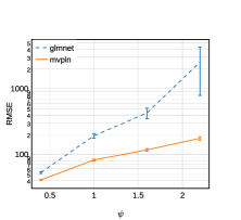
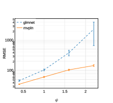
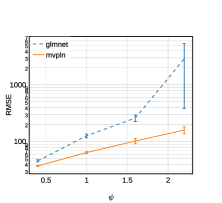
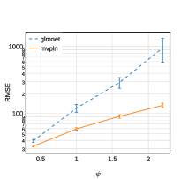
Figure 2: Average rMSE across response dimensions over test data when $\boldsymbol{\Omega}$ is random, sparse, banded and diagonal (from left to right), and $p<n$. The vertical error bars indicate the standard deviation, and the Y-axis is in log scale.

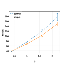
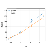
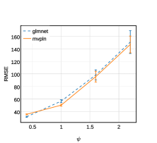
Figure 3: Average rMSE across response dimensions over test data when $\boldsymbol{\Omega}$ is random, sparse, banded and diagonal (from left to right), and $p\geq n$. The vertical error bars indicate the standard deviation.

3.1.2 Prediction errors

To evaluate the prediction performance of the proposed model, we report the average root-mean-square error (rMSE) across all the response dimensions over the test data. Figure 2 and 3 show the average rMSE for the cases when $p<n$ and $p\geq n$ respectively. These figures show that when the variations in the simulated data are small ($\psi$ is small), the prediction performances of the proposed MVPLN model and GLMNET model are comparable. As the variations in the data increase, the prediction performance of the proposed MVPLN model becomes better than GLMNET model. This demonstrates that by incorporating the dependency structures between the count responses, the proposed MVPLN model improves its prediction performance. However, when the variations in the data are small, it is difficult for the MVPLN model to take the advantage of inverse covariance matrix estimation. On the contrary, approximating the log-likelihood with MCMC techniques would impose negative effects on the model estimation and prediction accuracy. This is why we observe that when $\psi$ is small, the proposed MVPLN model sometimes does not perform as well as the GLMNET model in term of rMSE.

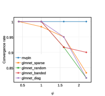
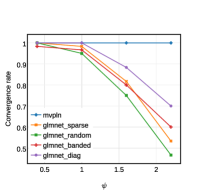
Figure 4: Convergence rate of GLMNET and MVPLN models when $p<n$ (left) and $p>n$ (right). Since MVPLN model always converges, we use a single line to represent these four scenarios.

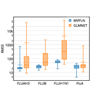
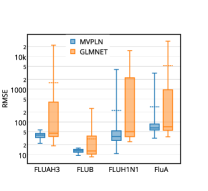
Figure 5: rMSE box plot of MVPLN and GLMNET models on the real ILI dataset for the countries of Brazil (left) and Chile (right). The dash lines indicate the mean of the rMSE.

3.1.3 Model convergence

Another aspect we would like to emphasize here is the model convergence performance. During the experiments over the simulated data, we notice that the GLMNET model will not always converge in some parameter settings, especially when $\psi$ is large. As a result, no parameter estimations are given by the GLMNET model. Figure 5 shows the convergence rate (the fraction of experiment replications that converge and produce valid model estimation) over the simulated data for various parameter settings. We can see from the figure that the larger variations (larger $\psi$) in the data, the more frequently the GLMNET model fails to give a valid model estimation. On the other hand, the proposed MVPLN model consistently produces the valid model estimation in all of the scenarios. Such results demonstrate that the proposed MVPLN model is more robust to the variations in the underlying multivariate data with count responses.

3.2 Modeling influenza-like illness case counts

We apply the proposed MVPLN model to a real influenza-like illness (ILI) dataset for two Latin American countries, Brazil and Chile, each with four types of ILI diseases (FLUAH3, FLUB, FLUH1N1 and FLUA). The data were collected from WHO FluNet [1] from May 1st, 2012 to Dec. 27, 2014 ($n=139$ weeks), which serves as the multivariate responses of the dataset. The predictors of this ILI dataset are the weekly counts of $108$ ILI related keywords collected from the Twitter users of Brazil and Chile during the same period. Before applying the proposed MVPLN model, we preprocessed the ILI dataset with the following approach. We first clustered the $108$ ILI related keywords into $20$ clusters based on their weekly counts during the selected period using the k-means algorithm. Then for each cluster, we aggregated the weekly counts together for the keywords that belong to this cluster, and finally, we scaled the aggregated keyword counts for each cluster so that it has zero mean and unit standard deviation.

It should also be noticed that although this ILI dataset is time-indexed, we chose to model it as merely a multivariate dataset in our first study here since the proposed MVPLN model is not specially designed to model time series datasets. We use $70\%$ of the preprocessed ILI dataset as the training set and the rest ($30\%$) as the test set. We apply the proposed MVPLN model over the training set , and compute the rMSE of the test set as the criterion for the prediction performance of the model. As a comparison, we also apply the GLMNET model to the same ILI dataset, and compare the rMSE with the proposed MVPLN model. We repeat this experiment for $60$ independent runs, and for each run, we shuffle the ILI dataset and re-split the training set and test set. Figure 5 shows the rMSE box plots of the proposed MVPLN model and the GLMNET model for Brazil and Chile after removing some extreme outliers. As we can see from the box plots, although the proposed MVPLN model generates slightly large rMSE over the test set for some response dimensions occasionally, in general, the rMSEs of the MVPLN model are much smaller and have less variation when compared to the GLMNET model for both Brazil and Chile, which indicates that the proposed MVPLN model is better and more stable in term of the prediction performance over the real dataset with count responses. Such results demonstrate that by leveraging the covariance structures between multiple count responses, the proposed MVPLN model improves the prediction performance. However, we also notice that for some flu types, the proposed MVPLN model sometimes generate a large rMSE value, e.g. FLUAH3 in the Brazil dataset, FLUH1N1 and FluA in the Chile dataset. The potential reason for this is likely that the data shuffling procedure happens to place most of the large-response data instances into the model training set, which could mislead the model estimation and result in an overestimation over the test set.

4 Conclusion

In this paper, we have proposed and formulated a multivariate Poisson log-normal model for datasets with count responses. By developing an MCEM algorithm, we accomplish simultaneous sparse estimations of the regression coefficients and of the inverse covariance matrix of the model. Results of simulation studies on synthetic data and an application to a real ILI dataset demonstrate that the proposed MVPLN model achieves better estimation and prediction performance versus a classical Lasso regularized Poisson regression model. Additional interesting future work for the proposed model are being conducted on the following lines. (1) Asymptotic properties of the proposed model are being further investigated; (2) instead of using MCMC techniques, we aim to develop a better approximation algorithm, e.g. using variational inference [4]; (3) we aim to develop variants of the proposed model to better deal with count data with over-dispersion and zero-inflation.

Appendix

Appendix A Distribution of multivariate count responses

Given the multivariate count response $\boldsymbol{\mathcal{Y}}$ and the predictor $\boldsymbol{x}$, with the conditional independence assumption, the probability mass function for the multivariate Poisson random variable $\boldsymbol{\mathcal{Y}}$ is

$$p(\boldsymbol{\mathcal{Y}}=\boldsymbol{y}\mid\boldsymbol{\theta})= \prod_{i=1}^{q}p(\mathcal{Y}^{(i)}=y^{(i)}\mid\theta^{(i)})=\prod_{i=1}^{q}\frac{{\left(\theta^{(i)}\right)}^{y^{(i)}}\exp\left(-\theta^{(i)}\right)}{y^{(i)}!}$$ (13)

From the specification of the MVPLN model, since $\boldsymbol{\varepsilon}\sim N(0,\boldsymbol{\Sigma})$, if we let $\boldsymbol{\gamma}=\boldsymbol{B}^{T}\boldsymbol{x}+\boldsymbol{\varepsilon}$, we know that $\boldsymbol{\gamma}$ follows the multivariate normal distribution $N(\boldsymbol{B}^{T}\boldsymbol{x},\boldsymbol{\Sigma})$ with density function:

$$p(\boldsymbol{\gamma}\mid\boldsymbol{x})=\frac{1}{{(2\pi)}^{q/2}{|\boldsymbol{\Sigma}|}^{1/2}}\exp\left(-\frac{1}{2}{(\boldsymbol{\gamma}-\boldsymbol{B}^{T}\boldsymbol{x})}^{T}\boldsymbol{\Sigma}^{-1}(\boldsymbol{\gamma}-\boldsymbol{B}^{T}\boldsymbol{x})\right)$$

Since $\boldsymbol{\theta}=\exp(\boldsymbol{\gamma})=\exp(\boldsymbol{B}^{T}\boldsymbol{x}+\boldsymbol{\varepsilon})$, $\boldsymbol{\theta}\mid\boldsymbol{x}$ follows the multivariate log-normal distribution, and we can derive that the density function of $\boldsymbol{\theta}\mid\boldsymbol{x}$ is:

$$p(\boldsymbol{\theta} \mid\boldsymbol{x})=p_{\boldsymbol{\gamma}}(\log(\boldsymbol{\theta})\mid\boldsymbol{x})\left|\operatorname{diag}\left(\frac{1}{\theta^{(i)}}\right)\right|=\frac{\exp\left(-\frac{1}{2}{\left(\log\boldsymbol{\theta}-\boldsymbol{B}^{T}\boldsymbol{x}\right)}^{T}\boldsymbol{\Sigma}^{-1}\left(\log\boldsymbol{\theta}-\boldsymbol{B}^{T}\boldsymbol{x}\right)\right)}{{(2\pi)}^{q/2}|\boldsymbol{\Sigma}|^{1/2}\prod_{i=1}^{q}\theta^{(i)}}.$$ (14)

Thus, the probability mass function for $\boldsymbol{\mathcal{Y}}\mid\boldsymbol{x}$ is:

$$p(\boldsymbol{\mathcal{Y}}=\boldsymbol{y}\mid\boldsymbol{x})= \int_{\boldsymbol{\theta}}p(\boldsymbol{\mathcal{Y}}=\boldsymbol{y},\boldsymbol{\theta}\mid\boldsymbol{x})d\boldsymbol{\theta}=\int_{\boldsymbol{\theta}}p(\boldsymbol{\mathcal{Y}}=\boldsymbol{y}\mid\boldsymbol{\theta})p(\boldsymbol{\theta}\mid\boldsymbol{x})d\boldsymbol{\theta},$$

where $p(\boldsymbol{\mathcal{Y}}=\boldsymbol{y}\mid\boldsymbol{\theta})$ and $p(\boldsymbol{\theta}\mid\boldsymbol{x})$ are specified in Equation (13) and (14), respectively.

Appendix B Monte Carlo E-step in MCEM algorithm

B.1 Metropolis Hasting algorithm for sampling $\boldsymbol{\theta}_{j}$

Suppose in the MC E-step of iteration $t+1$, the current estimations of the model parameters are $\boldsymbol{B}^{(t)}$ and $\boldsymbol{\Sigma}^{(t)}$. Thus, the conditional distribution of the latent variable $\boldsymbol{\theta}$ given $\boldsymbol{x},\boldsymbol{y},\boldsymbol{B}^{(t)}$ and $\boldsymbol{\Sigma}^{(t)}$ is:

$$p(\boldsymbol{\theta}\mid\boldsymbol{\mathcal{Y}}=\boldsymbol{y},\boldsymbol{x};\boldsymbol{B}^{(t)},\boldsymbol{\Sigma}^{(t)})=\frac{p(\boldsymbol{\mathcal{Y}}=\boldsymbol{y},\boldsymbol{\theta}\mid\boldsymbol{x};\boldsymbol{B}^{(t)},\boldsymbol{\Sigma}^{(t)})}{p(\boldsymbol{\mathcal{Y}}=\boldsymbol{y}\mid\boldsymbol{x};\boldsymbol{B}^{(t)},\boldsymbol{\Sigma}^{(t)})}.$$ (15)

1

input : $\boldsymbol{y}_{j},\boldsymbol{x}_{j},\boldsymbol{B}^{(t)}$ and $\boldsymbol{\Sigma}^{(t)}$.

output : $m$ samples $\boldsymbol{\Theta}_{j}={\left\{\boldsymbol{\theta}_{j}^{(1)},\boldsymbol{\theta}_{j}^{(2)},\ldots,\boldsymbol{\theta}_{j}^{(m)}\right\}}^{T}$.

2

3Choose $\boldsymbol{\theta}_{j}^{(0)}$ as initial value, and let $\tau\leftarrow 1$;

4 while $|\boldsymbol{\Theta}_{j}|<m$ do

5       Draw a candidate $\boldsymbol{\theta}_{j}^{*}$ from $g(\boldsymbol{\theta}_{j}^{*}\mid\boldsymbol{\theta}_{j}^{(\tau-1)})$;

6       $\alpha\leftarrow\min\left(\frac{f(\boldsymbol{\theta}_{j}^{*})/g(\boldsymbol{\theta}_{j}^{*}\mid\boldsymbol{\theta}_{j}^{(\tau-1)})}{f(\boldsymbol{\theta}_{j}^{(\tau-1)})/g(\boldsymbol{\theta}_{j}^{(\tau-1)}\mid\boldsymbol{\theta}_{j}^{*})},1\right)$;

7       Accept $\boldsymbol{\theta}_{j}^{(*)}$ as $\boldsymbol{\theta}_{j}^{(\tau)}$ with probability $\alpha$;

8       if $\boldsymbol{\theta}_{j}^{(*)}$ is accepted then

9             $\boldsymbol{\Theta}_{j}\leftarrow\boldsymbol{\Theta}_{j}\cup\{\boldsymbol{\theta}_{j}^{(\tau)}\}$;

10             $\tau\leftarrow\tau+1$;

11            

12       end if

13      

14 end while

15return $\boldsymbol{\Theta}_{j}$;

16

Algorithm 1 Metropolis Hasting algorithm for sampling $\boldsymbol{\theta}_{j}$

Then, the expected log-likelihood of the model under $p(\boldsymbol{\theta}\mid\boldsymbol{\mathcal{Y}}=\boldsymbol{y},\boldsymbol{x};\boldsymbol{B}^{(t)},\boldsymbol{\Sigma}^{(t)})$ would be:

$$Q(\boldsymbol{B},\boldsymbol{\Sigma} \mid\boldsymbol{B}^{(t)},\boldsymbol{\Sigma}^{(t)})=E_{p(\boldsymbol{\theta}\mid\boldsymbol{\mathcal{Y}}=\boldsymbol{y},\boldsymbol{x})}[\mathcal{L}(\boldsymbol{B},\boldsymbol{\Sigma})]$$ (16)

$$=\sum_{j=1}^{n}E_{p(\boldsymbol{\theta}_{j}\mid\boldsymbol{\mathcal{Y}}=\boldsymbol{y}_{j},\boldsymbol{x}_{j})}[\log p(\boldsymbol{\mathcal{Y}}=\boldsymbol{y}_{j},\boldsymbol{\theta}_{j}\mid\boldsymbol{x}_{j};\boldsymbol{B},\boldsymbol{\Sigma})].$$

In order to compute the approximate expected log-likelihood, we adopt the MCMC technique to sample the $\boldsymbol{\theta}_{j}$ from $p(\boldsymbol{\theta}_{j}\mid\boldsymbol{\mathcal{Y}}=\boldsymbol{y}_{j},\boldsymbol{x}_{j};\boldsymbol{B}^{(t)},\boldsymbol{\Sigma}^{(t)})$. Since $\boldsymbol{y}_{j},\boldsymbol{x}_{j},\boldsymbol{B}^{(t)}$ and $\boldsymbol{\Sigma}^{(t)}$ are all known values, which makes $p(\boldsymbol{\mathcal{Y}}=\boldsymbol{y}_{j}\mid\boldsymbol{x}_{j};\boldsymbol{B}^{(t)},\boldsymbol{\Sigma}^{(t)})$ a constant. In this case, Equation (15) yields

$$p(\boldsymbol{\theta}_{j}\mid\boldsymbol{\mathcal{Y}}=\boldsymbol{y}_{j}, \boldsymbol{x}_{j};\boldsymbol{B}^{(t)},\boldsymbol{\Sigma}^{(t)})\propto p(\boldsymbol{\mathcal{Y}}=\boldsymbol{y}_{j},\boldsymbol{\theta}_{j}\mid\boldsymbol{x}_{j};\boldsymbol{B}^{(t)},\boldsymbol{\Sigma}^{(t)}).$$

Let $f(\boldsymbol{\theta}_{j})=p(\boldsymbol{\mathcal{Y}}=\boldsymbol{y}_{j},\boldsymbol{\theta}_{j}\mid\boldsymbol{x}_{j};\boldsymbol{B}^{(t)},\boldsymbol{\Sigma}^{(t)})$ and $g(\boldsymbol{\theta}^{*}\mid\boldsymbol{\theta})$ be the density function of the proposal distribution. Algorithm 1 illustrates the Metropolis Hasting algorithm for sampling $\boldsymbol{\theta}_{j}$ from $p(\boldsymbol{\theta}_{j}\mid\boldsymbol{\mathcal{Y}}=\boldsymbol{y}_{j},\boldsymbol{x}_{j};\boldsymbol{B}^{(t)},\boldsymbol{\Sigma}^{(t)})$.

B.2 Derivation of the tailored normal distribution as proposal distribution

To find the mode of $p(\boldsymbol{\theta}_{j}\mid\boldsymbol{\mathcal{Y}}=\boldsymbol{y}_{j},\boldsymbol{x}_{j};\boldsymbol{B}^{(t)},\boldsymbol{\Sigma}^{(t)})$, we need to solve the following optimization problem:

$$\boldsymbol{\theta}_{j}^{(0)}=\operatornamewithlimits{argmax}_{\boldsymbol{\theta}_{j}}\{\log f(\boldsymbol{\theta}_{j})\},$$

let $F(\boldsymbol{\theta}_{j})=\log f(\boldsymbol{\theta}_{j})=\log\left(p(\boldsymbol{\mathcal{Y}}=\boldsymbol{y}_{j}\mid\boldsymbol{\theta}_{j},\boldsymbol{x}_{j};\boldsymbol{B}^{(t)},\boldsymbol{\Sigma}^{(t)})p(\boldsymbol{\theta}_{j}\mid\boldsymbol{x}_{j};\boldsymbol{B}^{(t)},\boldsymbol{\Sigma}^{(t)})\right)$. By combining Equation (13) and (14) together, we can derive that:

$$F(\boldsymbol{\theta}_{j}) ={(\boldsymbol{y}_{j}-\boldsymbol{1})}^{T}\log\boldsymbol{\theta}_{j}-\boldsymbol{1}^{T}\boldsymbol{\theta}_{j}-\frac{1}{2}{\left(\log\boldsymbol{\theta}_{j}-{\boldsymbol{B}^{(t)}}^{T}\boldsymbol{x}_{j}\right)}^{T}{\boldsymbol{\Sigma}^{(t)}}^{-1}\left(\log\boldsymbol{\theta}_{j}-{\boldsymbol{B}^{(t)}}^{T}\boldsymbol{x}_{j}\right)+C,$$ (17)

where $\boldsymbol{1}$ denotes a column vector of $1$s, and $C$ represents the sum of all the constants in $\log f(\boldsymbol{\theta}_{j})$. Then, the first order and second order derivatives of $F(\boldsymbol{\theta}_{j})$ w.r.t. $\boldsymbol{\theta}_{j}$ are

$$\nabla F(\boldsymbol{\theta}_{j})= \frac{dF(\boldsymbol{\theta}_{j})}{d\boldsymbol{\theta}_{j}}=\operatorname{diag}\left(\frac{1}{\theta_{j}^{(i)}}\right)\left[(\boldsymbol{y}_{j}-\boldsymbol{1})-{\boldsymbol{\Sigma}^{(t)}}^{-1}\left(\log\boldsymbol{\theta}_{j}-{\boldsymbol{B}^{(t)}}^{T}\boldsymbol{x}_{j}\right)\right]-\boldsymbol{1}$$ (18)

$$\boldsymbol{H}(\boldsymbol{\theta}_{j})= \operatorname{diag}\left(-\frac{y_{j}^{(i)}-1}{{\theta_{j}^{(i)}}^{2}}\right)+\operatorname{diag}\left(-\frac{1}{{\theta_{j}^{(i)}}^{2}}\right)\operatorname{diag}\left({\boldsymbol{\Sigma}^{(t)}}^{-1}\left(\log\boldsymbol{\theta}_{j}-{\boldsymbol{B}^{(t)}}^{T}\boldsymbol{x}_{j}\right)\right)$$

$$+\operatorname{diag}\left(\frac{1}{\theta_{j}^{(i)}}\right){\boldsymbol{\Sigma}^{(t)}}^{-1}\operatorname{diag}\left(\frac{1}{\theta_{j}^{(i)}}\right)$$ (19)

Let $\nabla F(\boldsymbol{\theta}_{j})=0$, and we could get that the initial value $\boldsymbol{\theta}_{j}^{(0)}$ of the location parameter for the tailored normal distribution is the solution to the following equation:

$$\boldsymbol{\theta}_{j}+{\boldsymbol{\Sigma}^{(t)}}^{-1}\log\boldsymbol{\theta}_{j}=\boldsymbol{y}_{j}-\boldsymbol{1}+{\boldsymbol{\Sigma}^{(t)}}^{-1}{\boldsymbol{B}^{(t)}}^{T}\boldsymbol{x}_{j}$$ (20)

which can be solved by any numerical root discovering algorithms. However, taking performance issue into account, we let $\boldsymbol{\kappa}_{j}=\log\boldsymbol{\theta}_{j}$, and adopt a linear approximation to $\boldsymbol{e}^{\boldsymbol{\kappa}_{j}}$ with its first order Taylor expansion at $\boldsymbol{\kappa}_{j}^{(0)}=\log\boldsymbol{y}_{j}$. In this case, Equation (20) becomes:

$$\boldsymbol{e}^{\boldsymbol{\kappa}_{j}^{(0)}}+\operatorname{diag}\left(\boldsymbol{e}^{\boldsymbol{\kappa}_{j}^{(0)}}\right)\left(\boldsymbol{\kappa}_{j}-\boldsymbol{\kappa}_{j}^{(0)}\right)+{\boldsymbol{\Sigma}^{(t)}}^{-1}\boldsymbol{\kappa}_{j}=\boldsymbol{y}_{j}-\boldsymbol{1}+{\boldsymbol{\Sigma}^{(t)}}^{-1}{\boldsymbol{B}^{(t)}}^{T}\boldsymbol{x}_{j}.$$ (21)

Solving Equation (21) for $\boldsymbol{\kappa}_{j}$, the location parameter (mean) $\boldsymbol{\theta}_{j}$ of the tailored normal distribution is given by $\boldsymbol{\theta}_{j}^{(0)}=\boldsymbol{e}^{\boldsymbol{\kappa}_{j}}$ where

$$\boldsymbol{\kappa}_{j}= {\left(\operatorname{diag}\left(\boldsymbol{e}^{\boldsymbol{\kappa}_{j}^{(0)}}\right)+{\boldsymbol{\Sigma}^{(t)}}^{-1}\right)}^{-1}\Big{(}\boldsymbol{y}_{j}-\boldsymbol{1}+{\boldsymbol{\Sigma}^{(t)}}^{-1}{\boldsymbol{B}^{(t)}}^{T}\boldsymbol{x}_{j}+\operatorname{diag}\left(\boldsymbol{e}^{\boldsymbol{\kappa}_{j}^{(0)}}\right)\boldsymbol{\kappa}_{j}^{(0)}-\boldsymbol{e}^{\boldsymbol{\kappa}_{j}^{(0)}}\Big{)},$$

and the covariance matrix is given by $\tau(-\boldsymbol{H}(\boldsymbol{\theta}_{j}^{(0)}))^{-1}$. In the case that the covariance matrix $\tau(-\boldsymbol{H}(\boldsymbol{\theta}_{j}^{(0)}))^{-1}$ is not positive semidefinite, the nearest positive semidefinite matrix to $\tau(-\boldsymbol{H}(\boldsymbol{\theta}_{j}^{(0)}))^{-1}$ is used to replace $\tau(-\boldsymbol{H}(\boldsymbol{\theta}_{j}^{(0)}))^{-1}$.

Appendix C M-step in the MCEM algorithm

C.1 The optimization problem in M-step

The joint distribution of $(\boldsymbol{\mathcal{Y}}=\boldsymbol{y}_{j},\boldsymbol{\theta}_{j}^{(\tau)})$ given $\boldsymbol{x}_{j},\boldsymbol{B}^{(t)}$ and $\boldsymbol{\Sigma}^{(t)}$ is:

$$p(\boldsymbol{\mathcal{Y}}=\boldsymbol{y}_{j},\boldsymbol{\theta}_{j}^{(\tau)}\mid\boldsymbol{x}_{j};\boldsymbol{B}^{(t)},\boldsymbol{\Sigma}^{(t)})=p(\boldsymbol{\mathcal{Y}}=\boldsymbol{y}_{j}\mid\boldsymbol{\theta}_{j}^{(\tau)})p(\boldsymbol{\theta}_{j}^{(\tau)}\mid\boldsymbol{x}_{j};\boldsymbol{B}^{(t)},\boldsymbol{\Sigma}^{(t)})$$

where $p(\boldsymbol{\mathcal{Y}}=\boldsymbol{y}_{j}\mid\boldsymbol{\theta}_{j}^{(\tau)})$ and $p(\boldsymbol{\theta}_{j}^{(\tau)}\mid\boldsymbol{x}_{j};\boldsymbol{B}^{(t)},\boldsymbol{\Sigma}^{(t)})$ are given by Equation (13) and (14) respectively. Let $\boldsymbol{\Omega}=\boldsymbol{\Sigma}^{-1}$ and $\boldsymbol{\varphi}_{\tau,j}=(\log\boldsymbol{\theta}_{j}^{(\tau)}-\boldsymbol{B}^{T}\boldsymbol{x}_{j})$. Combining the approximated expected log-likelihood we derived in the MC E-step in Section 2.2.1 (Equation (7) in the paper), we can reformulate $\tilde{Q}(\boldsymbol{B},\boldsymbol{\Sigma}\mid\boldsymbol{B}^{(t)},\boldsymbol{\Sigma}^{(t)})$ as:

$$\tilde{Q}(\boldsymbol{B},\boldsymbol{\Sigma}\mid\boldsymbol{B}^{(t)},\boldsymbol{\Sigma}^{(t)}) =-\frac{1}{n}\sum_{j=1}^{n}\frac{1}{m}\sum_{\tau=1}^{m}\bigg{[}{\left(\log\boldsymbol{\theta}_{j}^{(\tau)}-\boldsymbol{B}^{T}\boldsymbol{x}_{j}\right)}^{T}\boldsymbol{\Omega}\left(\log\boldsymbol{\theta}_{j}^{(\tau)}-\boldsymbol{B}^{T}\boldsymbol{x}_{j}\right)-\log|\boldsymbol{\Omega}|\bigg{]}$$

$$=-\frac{1}{mn}\operatorname{tr}\left(\boldsymbol{\Phi}^{T}\boldsymbol{\Phi}\boldsymbol{\Omega}\right)+\log|\boldsymbol{\Omega}|.$$ (22)

Then, the optimization problem we need to solve in the M-step is:

$$\boldsymbol{B}^{(t+1)},\boldsymbol{\Sigma}^{(t+1)} =\operatornamewithlimits{argmin}_{\boldsymbol{B},\boldsymbol{\Sigma}}\left\{-\tilde{Q}(\boldsymbol{B},\boldsymbol{\Sigma}\mid\boldsymbol{B}^{(t)},\boldsymbol{\Sigma}^{(t)})+\lambda_{1}||\boldsymbol{B}||_{1}+\lambda_{2}||\boldsymbol{\Sigma}^{-1}||_{1}\right\}$$

$$=\operatornamewithlimits{argmin}_{\boldsymbol{B},\boldsymbol{\Omega}}\left\{\frac{1}{mn}\operatorname{tr}\left(\boldsymbol{\Phi}^{T}\boldsymbol{\Phi}\boldsymbol{\Omega}\right)-\log|\boldsymbol{\Omega}|+\lambda_{1}||\boldsymbol{B}||_{1}+\lambda_{2}||\boldsymbol{\Omega}||_{1}\right\}$$ (23)

C.2 Approach to solve $\boldsymbol{B}$ approximately when $\boldsymbol{\Omega}$ fixed

When $\boldsymbol{\Omega}$ is fixed at $\boldsymbol{\Omega}_{0}$, we have the following convex optimization problem:

$$\boldsymbol{B}(\boldsymbol{\Omega}_{0})=\operatornamewithlimits{argmin}_{\boldsymbol{B}}\bigg{\{}\frac{1}{mn}\operatorname{tr}\left(\boldsymbol{\Phi}^{T}\boldsymbol{\Phi}\boldsymbol{\Omega}_{0}\right)+\lambda_{1}||\boldsymbol{B}||_{1}\bigg{\}}.$$ (24)

The $l_{1}$ matrix norm penalty in Equation (24) could be approximated with the following approach

$$||\boldsymbol{B}||_{1}\approx\operatorname{tr}\left({\boldsymbol{B}^{\prime}}^{T}\boldsymbol{B}^{\prime}\right),\quad\text{where}~{}\boldsymbol{B}^{\prime}=\boldsymbol{B}\circ\frac{1}{\sqrt{|\hat{\boldsymbol{B}}|}}.$$

Here, $\circ$ denotes the Hadamard (element-wise) product. If we write $\boldsymbol{\Phi}$ into the following block matrix

$$\boldsymbol{\Phi}=\left[\begin{array}[]{c}\log\boldsymbol{\Theta}_{1}-\boldsymbol{X}_{1}\boldsymbol{B}\\ \log\boldsymbol{\Theta}_{2}-\boldsymbol{X}_{2}\boldsymbol{B}\\ \vdots\\ \log\boldsymbol{\Theta}_{n}-\boldsymbol{X}_{n}\boldsymbol{B}\\ \end{array}\right],$$

where $\boldsymbol{X}_{j}$ is $m\times p$ matrix with each row being $\boldsymbol{x}_{j}$ for all $j=1,2,\ldots,n$, the objective function of the optimization problem in (24) can be written as:

$$\eta( \boldsymbol{B})=\lambda_{1}\operatorname{tr}\left({\boldsymbol{B}^{\prime}}^{T}\boldsymbol{B}^{\prime}\right)+\frac{1}{mn}\sum_{j=1}^{n}\operatorname{tr}\Big{(}{(\log\boldsymbol{\Theta}_{j}-\boldsymbol{X}_{j}\boldsymbol{B})}^{T}(\log\boldsymbol{\Theta}_{j}-\boldsymbol{X}_{j}\boldsymbol{B})\boldsymbol{\Omega}_{0}\Big{)}.$$ (25)

Taking the first order derivative of $\eta(\boldsymbol{B})$ w.r.t. $\boldsymbol{B}$ and setting it to zero, we have

$$\left(\sum_{j=1}^{n}\boldsymbol{X}_{j}^{T}\boldsymbol{X}_{j}\right)\boldsymbol{B}\boldsymbol{\Omega}_{0}+\boldsymbol{B}\circ\frac{\lambda_{1}mn}{|\hat{\boldsymbol{B}}|}=\left(\sum_{j=1}^{n}\boldsymbol{X}_{j}^{T}(\log\boldsymbol{\Theta}_{j})\right)\boldsymbol{\Omega}_{0}$$ (26)

If we let $\Big{(}\sum\limits_{j=1}^{n}\boldsymbol{X}_{j}^{T}(\log\boldsymbol{\Theta}_{j})\Big{)}\boldsymbol{\Omega}_{0}=\boldsymbol{H}$ and $\sum\limits_{j=1}^{n}\boldsymbol{X}_{j}^{T}\boldsymbol{X}_{j}=\boldsymbol{S}$, and apply the matrix vectorization operator $\operatorname{vec}(\cdot)$ to both sides of Equation (26), we have:

$$\left(\boldsymbol{\Omega}_{0}^{T}\otimes\boldsymbol{S}\right)\operatorname{vec}\left(\boldsymbol{B}\right)+\operatorname{vec}\left(\frac{\lambda_{1}mn}{|\hat{\boldsymbol{B}|}}\right)\circ\operatorname{vec}\left(\boldsymbol{B}\right)=\operatorname{vec}\left(\boldsymbol{H}\right).$$

Here, $\otimes$ represents the Kronecker product. By pulling $\operatorname{vec}(\boldsymbol{B})$ out from the left hand side of the above equation, we can get:

$$\left[\boldsymbol{\Omega}_{0}\otimes\boldsymbol{S}+\operatorname{diag}\left(\operatorname{vec}\left(\frac{\lambda_{1}mn}{|\boldsymbol{B}_{\mathit{est}}|}\right)\right)\right]\operatorname{vec}(\boldsymbol{B})=\operatorname{vec}(\boldsymbol{H}).$$

Thus, the solution to the optimization problem in Equation (24) is

$$\operatorname{vec}(\boldsymbol{B})={\left[\boldsymbol{\Omega}_{0}\otimes\boldsymbol{S}+\operatorname{diag}\left(\operatorname{vec}\left(\frac{\lambda_{1}mn}{|\hat{\boldsymbol{B}}|}\right)\right)\right]}^{-1}\operatorname{vec}(\boldsymbol{H}),$$ (27)

and the estimated coefficient matrix $\boldsymbol{B}$ can be obtained by reorganizing the $\operatorname{vec}(\boldsymbol{B})$ in the above equation.

C.3 Algorithm pseudo code for M-step

By solving $\boldsymbol{B}$ and $\boldsymbol{\Omega}$ alternatively with the other fixed at the value of the last estimate until convergence, we will obtain the MLE of the coefficient matrix $\boldsymbol{B}$ and inverse covariance matrix $\boldsymbol{\Omega}$ for the current iteration of MCEM algorithm. Algorithm 2 summarizes the M-step of the MCEM algorithm.

1

input : $\boldsymbol{X},\{\boldsymbol{\Theta}_{j}\},\boldsymbol{\Omega}_{0},\boldsymbol{B}_{0},\lambda_{1}$ and $\lambda_{2}$.

output : MLE of $\boldsymbol{B}$ and $\boldsymbol{\Omega}$.

2

3$t\leftarrow-1$;

4 repeat

5       $t\leftarrow t+1$;

6       $\boldsymbol{\Phi}\leftarrow\left[\begin{array}[]{c}\log\boldsymbol{\Theta}_{1}-\boldsymbol{X}_{1}\boldsymbol{B}^{(t)}\\ \log\boldsymbol{\Theta}_{2}-\boldsymbol{X}_{2}\boldsymbol{B}^{(t)}\\ \vdots\\ \log\boldsymbol{\Theta}_{n}-\boldsymbol{X}_{n}\boldsymbol{B}^{(t)}\\ \end{array}\right]$;

7       $\boldsymbol{\Omega}^{(t+1)}\leftarrow$ Graphical_Lasso($\boldsymbol{\Phi},\lambda_{2}$);

8       $\boldsymbol{S}\leftarrow\sum_{j=1}^{n}\boldsymbol{X}_{j}^{T}\boldsymbol{X}_{j}$;

9       $\boldsymbol{H}\leftarrow\sum_{j=1}^{n}\boldsymbol{X}_{j}^{T}(\log\boldsymbol{\Theta}_{j})\boldsymbol{\Omega}^{(t+1)}$;

10      

$$\boldsymbol{B}^{(t+1)}\leftarrow\bigg{[}\boldsymbol{\Omega}^{(t+1)}\otimes\boldsymbol{S}+\operatorname{diag}\left(\operatorname{vec}\left(\frac{\lambda_{1}mn}{|\boldsymbol{B}^{(t)}|}\right)\right)\bigg{]}^{-1}\operatorname{vec}(\boldsymbol{H});$$

11until convergence;

12return ($\boldsymbol{B}^{(t+1)},\boldsymbol{\Omega}^{(t+1)})$;

13

Algorithm 2 M-step of the MCEM algorithm

References

- who [2015] WHO FluNet, 2015. http://www.who.int/influenza/gisrs_laboratory/flunet/en/.
- Argyriou et al. [2007a] A. Argyriou, T. Evgeniou, and M. Pontil. Multi-task feature learning. In NIPS, pages 41–48, 2007a.
- Argyriou et al. [2007b] A. Argyriou, C. A. Micchelli, M. Pontil, and Y. Ying. A spectral regularization framework for multi-task structure learning. In NIPS, 2007b.
- Blei et al. [2016] D. M. Blei, A. Kucubelbir, and J. D. McAuliffe. Variational inference: A review for statisticians, 2016. https://arxiv.org/abs/1601.00670.
- Chen and Chen [2008] J. Chen and Z. Chen. Extended Bayesian information criteria for model selection with large model spaces. Biometrika, 95(3):759–771, 2008.
- Chen et al. [2011] J. Chen, J. Zhou, and J. Ye. Integrating low-rank and group-sparse structures for robust multi-task learning. In KDD ’11, pages 42–50, 2011.
- Chib et al. [1998] S. Chib, E. Greenberg, and R. Winkelmann. Posterior simulation and bayes factors in panel count data models. Journal of Econometrics, 86(1):33 – 54, 1998.
- El-Basyouny and Sayed [2009] K. El-Basyouny and T. Sayed. Collision prediction models using multivariate poisson-lognormal regression. Accident Analysis and Prevention, 41(4):820 – 828, 2009.
- Foygel and Drton [2010] R. Foygel and M. Drton. Extended bayesian information criteria for gaussian graphical models. In NIPS, pages 604–612, 2010.
- Friedman et al. [2007] J. Friedman, T. Hastie, H. Höfling, and R. Tibshirani. Pathwise coordinate optimization. The Annals of Applied Statistics, 1(2):302–332, 2007.
- Friedman et al. [2008] J. Friedman, T. Hastie, and R. Tibshirani. Sparse inverse covariance estimation with the graphical lasso. Biostatistics, 9(3):432–441, July 2008.
- Friedman et al. [2014] J. Friedman, T. Hastie, N. Simon, and R. Tibshirani. Lasso and elastic-net regularized generalized linear models, 2014. URL http://cran.r-project.org/web/packages/glmnet/glmnet.pdf.
- Gong et al. [2012a] P. Gong, J. Ye, and C. shui Zhang. Multi-stage multi-task feature learning. In NIPS, 2012a.
- Gong et al. [2012b] P. Gong, J. Ye, and C. Zhang. Robust multi-task feature learning. In KDD ’12, pages 895–903, 2012b.
- Gong et al. [2014] P. Gong, J. Zhou, W. Fan, and J. Ye. Efficient multi-task feature learning with calibration. In KDD ’14, pages 761–770, 2014.
- Hadiji et al. [2015] F. Hadiji, A. Molina, S. Natarajan, and K. Kersting. Poisson dependency networks: Gradient boosted models for multivariate count data. Machine Learning, 100(2):477–507, 2015.
- Higham [2002] N. J. Higham. Computing the nearest correlation matrix — a problem from finance. IMA Journal of Numer. Anal., 22(3):329–343, 2002.
- Jalali et al. [2010] A. Jalali, S. Sanghavi, C. Ruan, and P. K. Ravikumar. A dirty model for multi-task learning. In NIPS, pages 964–972, 2010.
- Karlis [2003] D. Karlis. An em algorithm for multivariate poisson distribution and related models. Journal of Applied Statistics, 30(1):63–77, 2003.
- Kumar and Daumé III [2012] A. Kumar and H. Daumé III. Learning task grouping and overlap in multi-task learning. In ICML ’12, 2012.
- Levina et al. [2008] E. Levina, A. Rothman, J. Zhu, et al. Sparse estimation of large covariance matrices via a nested lasso penalty. The Annals of Applied Statistics, 2(1):245–263, 2008.
- Liu et al. [2014] H. Liu, L. Wang, and T. Zhao. Multivariate regression with calibration. In NIPS, pages 127–135, 2014.
- Lozano et al. [2013] A. C. Lozano, H. Jiang, and X. Deng. Robust sparse estimation of multiresponse regression and inverse covariance matrix via the l2 distance. In KDD ’13, pages 293–301, 2013.
- Ma et al. [2008] J. Ma, K. M. Kockelman, and P. Damien. A multivariate Poisson-lognormal regression model for prediction of crash counts by severity, using Baysian methods. Accident Analysis and Prevention, 40:964–975, 2008.
- Rothman et al. [2010] A. J. Rothman, E. Levina, and J. Zhu. Sparse multivariate regression with covariance estimation. Journal of Computational and Graphical Statistics, 19(4):947–962, 2010.
- Wang et al. [2007] H. Wang, M. U. Kalwani, and T. Akçura. A bayesian multivariate poisson regression model of cross-category store brand purchasing behavior. Journal of Retailing & Consumer Services, 14(6):369–382, 2007.
- Wang et al. [2013] W. Wang, Y. Liang, and E. P. Xing. Block regularized lasso for multivariate multi-response linear regression. In AISTATS, pages 608–617, 2013.
- Wang et al. [2015] Z. Wang, P. Chakraborty, S. R. Mekaru, J. S. Brownstein, J. Ye, and N. Ramakrishnan. Dynamic poisson autoregression for influenza-like-illness case count prediction. In KDD ’15, pages 1285–1294, 2015.
- Wytock and Kolter [2013] M. Wytock and J. Z. Kolter. Sparse gaussian conditional random fields: Algorithms, theory, and application to energy forecasting. In ICML ’13, pages 1265–1273, 2013.
- Yang et al. [2013] E. Yang, P. K. Ravikumar, G. I. Allen, and Z. Liu. On poisson graphical models. In NIPS ’13. 2013.
- Yu et al. [2007] S. Yu, V. Tresp, and K. Yu. Robust multi-task learning with t-processes. In ICML ’07, 2007.