Conformal Bootstrap Dashing Hopes of Emergent Symmetry

Abstract

We use the conformal bootstrap program to derive necessary conditions for emergent symmetry enhancement from discrete symmetry (e.g. $\mathbb{Z}_{n}$) to continuous symmetry (e.g. $U(1)$) under the renormalization group flow. In three dimensions, in order for $\mathbb{Z}_{2}$ symmetry to be enhanced to $U(1)$ symmetry, the conformal bootstrap program predicts that the scaling dimension of the order parameter field at the infrared conformal fixed point must satisfy $\Delta_{1}>1.08$. We also obtain the similar conditions for $\mathbb{Z}_{3}$ symmetry with $\Delta_{1}>0.580$ and $\mathbb{Z}_{4}$ symmetry with $\Delta_{1}>0.504$ from the simultaneous conformal bootstrap analysis of multiple four-point functions. Our necessary conditions impose severe constraints on many controversial physics such as the chiral phase transition in QCD, the deconfinement criticality in Néel-VBS transitions and anisotropic deformations in critical $O(n)$ models. In some cases, we find that the conformal bootstrap program dashes hopes of emergent symmetry enhancement proposed in the literature.

I Introduction

Symmetry in nature is the most helpful guideline to understand physics. Beauty of the symmetry is that it may not have a microscopic origin, but it may appear as an emergent phenomenon. Such emergent symmetry plays a significant role in theoretical physics.

Take a lattice system for example. Suppose the defining Hamiltonian possesses certain discrete or continuous symmetry. This does not mean that the infrared (IR) physics has the same symmetry. Rather, it often shows enhanced symmetry, especially when the system is at criticality. Indeed, emergence of global continuous symmetry out of discrete lattice symmetry is ubiquitous in strongly interacting systems, and it has played a key role in understanding the nature of quantum criticality that is outside the scope of the traditional Wilson-Landau-Ginzburg (WLG) paradigm of phase transitions Senthil et al. (2004a, b).

In this paper, we derive universal necessary conditions for such emergent symmetry enhancement from discrete symmetry to continuous symmetry under the renormalization group (RG) flow by using the recently developed technique of numerical conformal bootstrap program in three-dimensions El-Showk et al. (2012); Kos et al. (2014a); El-Showk et al. (2014); Kos et al. (2014b); Nakayama and Ohtsuki (2014, 2015); Simmons-Duffin (2015); Kos et al. (2015); Iliesiu et al. (2015). We will show that the conformal symmetry imposes a strong constraint on when the emergent symmetry enhancement can or cannot occur.

Let us rephrase the question in terms of conformal field theories (CFTs). Suppose we have a system with emergent $U(1)$ symmetry in the IR. Can we realize the same system with smaller discrete symmetry (e.g. $\mathbb{Z}_{2}\in U(1)$) without fine-tuning? The $\mathbb{Z}_{2}$ symmetry forbids the perturbation of the $U(1)$ symmetric fixed point under the smallest charged operators that are $\mathbb{Z}_{2}$ odd. However, with the only $\mathbb{Z}_{2}$ symmetry, one cannot forbid a perturbation by twice $U(1)$ charged operators that are $\mathbb{Z}_{2}$ even. In order to obtain the emergent $U(1)$ symmetry, all the $\mathbb{Z}_{2}$ even but $U(1)$ charged operators must be irrelevant. The conformal bootstrap program tells exactly when this can happen. In this case, we find that the scaling dimension of the $\mathbb{Z}_{2}$ odd order parameter field must satisfy $\Delta_{1}>1.08$ in three dimensions. Otherwise, we always have $\mathbb{Z}_{2}$ even but $U(1)$ charged relevant deformations that we cannot forbid without fine-tuning.

Prior to our work, hopes of the emergent symmetries have relied on explicit ultraviolet Lagrangian or Hamiltonian with naive dimensional counting, or, at best, with the perturbative computations e.g. large $N$ expansions or $\epsilon$ expansions. Our necessary conditions from the conformal bootstrap program are non-perturbative, rigorous and universal, so they should be applied to any critical phenomena in nature as long as the conformal symmetry is realized at the fixed point.

In this paper, among many possibilities, we offer applications to two widely discussed controversies in the theoretical physics community. The one is finite temperature chiral phase transition in Quantum Chromo Dynamics (QCD) and the other is the deconfinement criticality in Néel-Valence Bond Solid (VBS) transitions. We also test our necessary conditions against anisotropic deformations of $O(n)$ critical vector models. In certain cases, we find that the conformal bootstrap program dashes hopes of emergent symmetry enhancement proposed in the literature.

II Necessary conditions for emergent symmetry enhancement from conformal bootstrap

The foremost basis of our claim is the conformal hypothesis: under the RG flow, the system reaches a critical point described by a unitary CFT. In particular, not only scale symmetry but also Lorentz and special conformal symmetry should emerge. The hypothesis seems to be valid in many classical as well as quantum critical systems as long as we trust the effective field theory description with emergent Lorentz symmetry. In particular, in the examples we will study in section III, there are no perturbative candidates for the Virial current in the effective action, which is the obstruction for conformal invariance in scale invariant field theory, so the scale invariance most likely implies conformal invariance. See e.g. Nakayama (2015) for a review on this argument.

Once conformal invariance is assumed, we may study the consistency of four-point functions that results in the conformal bootstrap equations. In our case, we are interested in the consistency of four-point functions $\langle O_{q}O^{\dagger}_{q}O_{q^{\prime}}O^{\dagger}_{q^{\prime}}\rangle$ of $U(1)$ charge $q$ local scalar operators $O_{q}$, whose scaling dimension is denoted by $\Delta_{q}$, with the crossing equations and unitarity, whose idea was first developed in four dimensional CFTs in Rattazzi et al. (2011). By mapping the crossing equations in unitary CFTs to a semi-definite problem, numerical optimization yields a bound on the scaling dimension of the operators that appear in the operator product expansion (OPE) e.g. $O_{q}\times O_{q^{\prime}}\sim O_{q+q^{\prime}}$. See Appendix A for the details of our implementation.

Let us begin with emerging $U(1)$ symmetry from $\mathbb{Z}_{2}$. The upper bound on $\Delta_{2}$ as a function of $\Delta_{1}$ in $U(1)$ symmetric CFTs is straightforwardly obtained as in Kos et al. (2014b) by studying $\langle O_{1}O_{1}^{\dagger}O_{1}O_{1}^{\dagger}\rangle$. The plot in Fig.1 shows the necessary condition $\Delta_{1}>1.08$ for the symmetry enhancement as the bound when $\Delta_{2}$ can be larger than $3$, at which point $O_{2}$ may become irrelevant. In other words, when $\Delta_{1}<1.08$, $O_{2}$ is always relevant and symmetry enhancement does not occur.

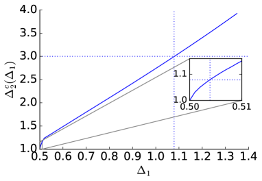
Figure 1: The upper bound on the scaling dimension $\Delta^{c}_{2}$ of the lowest dimensional charge two scalar operator appearing in $O_{1}\times O_{1}$ OPE as a function of $\Delta_{1}$. The same bound applies to $O_{2}\times O_{2}\sim O_{4}$.

For the $\mathbb{Z}_{3}$ enhancement, we study the simultaneous consistency of three four-point functions $\langle O_{1}O_{1}^{\dagger}O_{1}O_{1}^{\dagger}\rangle$, $\langle O_{1}O_{1}^{\dagger}O_{2}O_{2}^{\dagger}\rangle$ and $\langle O_{2}O_{2}^{\dagger}O_{2}O_{2}^{\dagger}\rangle$ from the mixed correlator conformal bootstrap analysis Kos et al. (2015); Lemos and Liendo (2016). In order to make the bound relevant for us, we make two additional assumptions: (1) all the charge four operators are irrelevant (2) all the charge neutral operators (above the identity) have scaling dimension larger than $1.044$. The latter assumption is motivated from our setup because it is easy to numerically prove it by using the conformal bootstrap analysis that if there exists a neutral scalar operator with scaling dimension less than $1.044$, there also exists another neutral scalar operator whose scaling dimension is less than 3 (see Appendix C for details). However, in all of our applications, there is only one neutral scalar operator that must be tuned, so the assumption is justifiable.

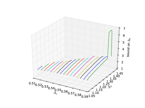
Figure 2: Upper Bounds on the scaling dimension of the lowest dimensional charge three scalar operator appearing in $O_{1}\times O_{2}$ OPE as a function of $\Delta_{1}$ and $\Delta_{2}$. The jump in the bounds appears as soon as they touch the value 3. Note that $1.08<\Delta_{2}<\Delta^{c}_{2}(\Delta_{1})$ must hold from the assumption that all the charge four operators are irrelevant and the bound in Fig.1.

Fig.2 shows the bound on $\Delta_{3}$ as a function of $\Delta_{1}$ and $\Delta_{2}$. When $\Delta_{1}\geq 0.585$, there exists an allowed region of $\Delta_{2}$ where $\Delta_{3}$ can be irrelevant. As soon as the bound on $\Delta_{3}$ touches $3$, it shows a conspicuous jump that is similar to the one observed in the fermionic conformal bootstrap analysis Iliesiu et al. (2015). Without knowing the value of $\Delta_{2}$, the plot shows that the necessary condition is $\Delta_{1}>0.580$. See Appendix D for two-dimensional projections of the plot.

In the similar manner, we can study the bound on $\Delta_{4}$ for the $\mathbb{Z}_{4}$ enhancement. We obtain the simplest bound by studying $\langle O_{1}O_{1}^{\dagger}O_{1}O_{1}^{\dagger}\rangle$ and $\langle O_{2}O_{2}^{\dagger}O_{2}O_{2}^{\dagger}\rangle$ independently, which immediately gives $\Delta_{1}>0.504$ (see Fig.1). The study of the simultaneous consistency of three four-point functions $\langle O_{1}O_{1}^{\dagger}O_{1}O_{1}^{\dagger}\rangle$, $\langle O_{1}O_{1}^{\dagger}O_{2}O_{2}^{\dagger}\rangle$ and $\langle O_{2}O^{\dagger}_{2}O_{2}O_{2}^{\dagger}\rangle$ gives a stronger bound in principle, but in practice, without introducing further assumptions, it does not improve much.

III Applications

III.1 Chiral phase transition in QCD

The order of chiral phase transition in finite temperature QCD has been controversial over many years without reaching a consensus. In the WLG paradigm, we may translate the problem into (non-)existence of RG fixed point in a certain three-dimensional WLG model whose order parameter is given by the quark bilinear “meson” field $\Phi_{\bar{i}j}=\bar{\psi}_{\bar{i}}\psi_{j}$ (where $\bar{i},j=1,2$ runs the number of “massless quarks” in nature). To reveal the nature of the RG flow, it is crucial to discuss whether the anomalous $U(1)_{A}$ symmetry is restored in the IR limit of the effective WLG model. If the $U(1)_{A}$ symmetry is restored, we expect that the chiral phase transition is described by an RG fixed point with the symmetry of $O(4)\times U(1)_{A}$ Pelissetto and Vicari (2013); Nakayama and Ohtsuki (2015). Otherwise, it is described by RG flow only with the symmetry of $O(4)$ Pisarski and Wilczek (1984). Here $O(4)\sim SU(2)_{R}\times SU(2)_{L}$ is the non-anomalous flavor symmetry of two massless quarks.

In Aoki et al. (2012, 2014); Kanazawa and Yamamoto (2016), it was shown that under mild assumptions, $\mathbb{Z}_{2}$ subgroup of the anomalous $U(1)_{A}$ is microscopically restored, which raises the second question if the $\mathbb{Z}_{2}$ can be further enhanced to the full $U(1)_{A}$ under the RG flow of the effective WLG model in three dimensions. This is exactly the problem we have discussed in section II, and the conformal bootstrap program gives a definite answer.

A study of the RG properties of this effective WLG model is notoriously hard, but the conformal bootstrap analysis of Nakayama and Ohtsuki (2015) tells that the scaling dimension of the $\mathbb{Z}_{2}$ odd operator at the $O(4)\times U(1)_{A}$ symmetric fixed point is $\Delta_{1}=0.82(2)$ (see Appendix B for more details). It turns out that this value does not satisfy the necessary condition for the $U(1)$ symmetry enhancement that we have derived in section II. We therefore conclude that the microscopic $O(4)\times\mathbb{Z}_{2}$ symmetry cannot be enhanced to $O(4)\times U(1)_{A}$ without fine-tuning. It means that the chiral phase transition in QCD does not accompany the full restoration of the $U(1)_{A}$ symmetry and does not show the second order phase transition described by the fixed point studied in Pelissetto and Vicari (2013); Nakayama and Ohtsuki (2015) unless further symmetry enhancement is assumed.

III.2 Deconfinement criticality in Néel-VBS transitions

The deconfinement criticality in Néel-VBS transitions in $2+1$ dimensions is proposed to be an example of critical phenomena whose description is beyond the traditional framework of WLG effective field theory. In Senthil et al. (2004a, b), they argued that the effective field theory description with $N$ component spin near the critical point is given by the non-compact $CP^{N-1}$ model Halperin et al. (1974); Kamal and Murthy (1993); Motrunich and Vishwanath (2004), or a $U(1)$ gauge theory coupled with $N$ charged scalars with $SU(N)$ flavor symmetry. While there has been no rigorous proof, it was argued that the system shows a conformal behavior once one can tune one parameter, the bare mass of the charged scalars.

However, it turns out that the actual realization of this critical behavior in the lattice simulation has been controversial over years. From the effective field theory viewpoint, a difficulty comes from the existence of monopole operators. One can argue that the lattice symmetry forbids the smallest charged monopole operator, but not necessarily so for the higher charged monopole operators Block et al. (2013); Harada et al. (2013). For instance, if we use the rectangular lattice, one can only preserve the $\mathbb{Z}_{2}$ subgroup of the $U(1)$ monopole charge, and if we use the honeycomb lattice it is $\mathbb{Z}_{3}$ and if we use the square lattice it is $\mathbb{Z}_{4}$. If the higher charged monopole operators that are not forbidden by the lattice symmetry are relevant, then we cannot reach the non-compact $CP^{N-1}$ model in the IR limit without further fine-tuning, and we typically expect the first order phase transition in lattice simulations.

Therefore the central question we should address is under which condition, the higher charged monopole operators become irrelevant once we know the scaling dimension of the lowest monopole charged operator. Again this is precisely the question we have studied in section II. To reiterate our results, in order to obtain $U(1)$ symmetry enhancement, we need $\Delta_{1}>1.08$ from $\mathbb{Z}_{2}$, $\Delta_{1}>0.580$ from $\mathbb{Z}_{3}$ and $\Delta_{1}>0.504$ from $\mathbb{Z}_{4}$.

In the following, we critically review various predictions about the nature of Néel-VBS phase transitions in the literature for different $N$. We may find a convenient summary of the scaling dimensions of operators proposed in the literature in Appendix B.

Let us begin with the $N=2$ case, which has the most experimental significance. The predictions of $\Delta_{1}$ in the literature ranges between $0.57$ and $0.68$. For whichever values, our necessary condition for $\mathbb{Z}_{4}$ tells that the charge four operators can be irrelevant and it is consistent with the observation of the second order phase transition on the square lattice. On the other hand, our necessary condition $\Delta_{1}>1.08$ for $\mathbb{Z}_{2}$ tells that the charge two monopole operator is relevant so we expect the first order phase transition on the rectangular lattice as observed indeed in Block et al. (2013).

The most controversial question is if the charge three monopole operator is relevant or not. Our necessary condition $\Delta_{1}>0.580$ is consistent with that it is either relevant or irrelevant, depending on the value of $\Delta_{1}$. We note that the scaling dimensions obtained in Sreejith and Powell (2015) (i.e. $\Delta_{1}=0.579(8),\Delta_{2}=1.42(7)$ and $\Delta_{3}=2.80(3)$) are very close to the bound. In particular, our results show that, given their values of $\Delta_{1}$ and $\Delta_{2}$, the charge three monopole operator must be relevant, supporting their claim that they observed the first order phase transition on the honeycomb lattice.

Let us next consider the $N=3$ case. In Harada et al. (2013), they obtained $\Delta_{1}=0.785$, so our necessary condition implies that it can show the second order phase transition on the square lattice but it cannot on the rectangular lattice, in agreement with what is observed. The direct measurement of $\Delta_{2}=2.0$ there turns out to be close to but slightly below our bound with $\Delta_{1}=0.785$. However, we also note that the earlier estimate of $\Delta_{1}=0.71(2)$ in Lou et al. (2009) may be inconsistent with $\Delta_{2}=2.0$.

For $N=4$, our result reveals inconsistency among the literature. In Harada et al. (2013) they obtained $\Delta_{1}=0.865$, and our condition predicts that the charge two monopole operator is relevant. On the other hand in Block et al. (2013), they claim that the charge two monopole operator is irrelevant and the phase transition is second order on the rectangular lattice. These statements cannot be mutually consistent, and one of them or our conformal hypotheses must be wrong.

For $N=5$, the situation is again subtle. Block et al. (2013) claims that it shows the second order phase transition on the rectangular lattice. Our result then demands that $\Delta_{1}>1.08$ to make charge two monopole operator irrelevant. The values they obtained on square and honeycomb lattices $\Delta_{1}=1.0(1)$ are quite marginal. In contrast, the value of $\Delta_{1}=0.85(1)$ they obtained on rectangular lattice is clearly inconsistent, so it is likely that the charge two monopole operator is actually relevant and the phase transition on the rectangular lattice may be first order.

Finally, for $N\geq 6$, the results in Block et al. (2013) as well as $1/N$ expansions (see e.g. Metlitski et al. (2008)) seem to suggest $\Delta_{1}>1.08$. Then our necessary condition implies that charge two monopole operators can be irrelevant and the phase transition on the rectangular lattice can be second order in agreement with the claims in the literature.

III.3 Anisotropic deformations in critical $O(n)$ models

Critical $O(n)$ vector models are canonical examples of conformal fixed points naturally realized in the WLG effective field theory. Under the RG flow, the $O(n)$ critical point is achieved by adjusting one parameter that is $O(n)$ singlet (e.g. temperature), but the fixed point may be unstable under anisotropic deformations. The stability under anisotropic deformations is an example of emergent symmetry and is subject to our general discussions.

Let us focus on $n=2$ (i.e XY model). It is believed that the $O(2)$ invariant conformal fixed point is unstable under anisotropic deformations with charge $q=2$ and $q=3$, but stable under $q\geq 4$ deformations. Our current best estimate based on the Monte-Carlo (MC) simulation is $\Delta_{1}=0.51905(10)$ and $\Delta_{2}=1.2361(11)$ Campostrini et al. (2006). These values are in agreement with the conformal bootstrap analysis of $O(2)$ invariant CFTs in Kos et al. (2014a, 2015). The MC simulations on scaling dimensions of $q=3$ and $q=4$ deformations are also available in Hasenbusch and Vicari (2011) as $\Delta_{3}=2.103(15)$ and $\Delta_{4}=3.108(6)$.

Now given $\Delta_{1}$ and $\Delta_{2}$, our conformal bootstrap program gives a rigorous upper bound on $\Delta_{3}$. With more precise data to be compared, we have tried to derive the more precise bound by increasing the approximation in our conformal bootstrap program (i.e. $\Lambda=23$: see Appendix A). The resulting bound is $\Delta_{3}<2.118$ for $\Delta_{1}=0.51905$ and $\Delta_{2}=1.234$. It turns out that the number quoted above is very close to (or almost saturating) the bound we have obtained.

On the other hand, the estimate of $\Delta_{4}=3.108(6)$ seems a little below the conformal bootstrap bound $\Delta_{4}<3.52$. It is not obvious if our bound is saturated but it is at least consistent that our conformal bootstrap bound does not predict that $q=4$ anisotropy must be relevant.

For $n>2$, it is a challenging problem to determine exactly when the cubic anisotropy becomes irrelevant. In the large $n$ limit, the cubic anisotropy is believed to be relevant, but for smaller $n$ it is believed to become irrelevant, showing the enhanced $O(n)$ symmetry. The current estimate of the critical $n$ is around $n=3$ (see e.g. Carmona et al. (2000)). However it is still an open question if it is strictly smaller than $3$.

Our conformal bootstrap program might shed some light on this problem. Repeating our analysis now with $O(n)$ symmetry rather than $U(1)$ on the four-point functions $\langle O_{[ij]}O_{[kl]}O_{[mn]}O_{[pq]}\rangle$, we can rigorously show that the cubic anisotropy must be relevant for $n=10$ with no assumptions and for $n=6$ with mild assumptions (e.g. non-conserved vector operators have scaling dimension larger than 3). For $n=3$ and $n=4$, the conformal bootstrap bound we have obtained is not conclusive yet.

IV Discussions

In this paper, we have numerically proved necessary conditions for emergent symmetry enhancement from discrete symmetry to continuous symmetry under the RG flow. Our conditions are universally valid, but given a concrete model with concrete predictions on critical exponents, we may be able to offer more stringent bounds. Even a modest partial data such as $\Delta_{0}=3-1/\nu$ will make the constraint more non-trivial. We are delighted to test consistency of future predictions obtained from the other methods upon request.

The symmetry enhancement we have discussed is mainly $U(1)$, but it is possible to discuss non-Abelian enhancement as well from the conformal bootstrap program. For example, there is an interesting conjecture Xu and Sachdev (2008)Nahum et al. (2015) that the non-compact $CP^{1}$ model shows further symmetry enhancement to $SO(5)$ by combining Néel order parameter and VBS order parameter. However, the conformal bootstrap analysis tells that the currently observed value of $\Delta_{1}$ (i.e. $\eta_{\mathrm{VBS}}\simeq\eta_{\text{N\'{e}el}}$) is too small for the conjecture to hold that it has no $SO(5)$ singlet relevant deformation.

Finally, we should stress that our discussions are entirely based on the emergent conformal symmetry. In quantum critical systems, this is more non-trivial than in classical critical systems. While the Lorentz invariant conformal fixed points are typically stable under Lorentz breaking deformations allowed on the lattice, it would be important to understand precisely under which condition, the conformal symmetry emerges.

Appendix A Technical details about conformal bootstrap implementation

The mathematical basis of the numerical conformal bootstrap program is the crossing symmetry of four-point functions in CFTs. In CFTs, we can expand he four-point functions by using the OPE

$$O_{i}\times O_{j}\sim\sum_{O}\lambda_{ijO}O,$$ (1)

$$O_{i}\times O_{j}^{\dagger}\sim\sum_{O}\lambda_{i\bar{j}O}O\ ,$$ (2)

where the assumption of unitarity dictates a reality condition on the OPE coefficient: $\lambda_{ijk}^{*}=\lambda_{\bar{i}\bar{j}\bar{k}}$,

In our problems, the crossing symmetry of four-point functions $\langle O_{i}O_{i}^{\dagger}O_{i}O_{i}^{\dagger}\rangle$ $(i=1,2)$ leads to equations

$$\sum_{O\in O_{i}\times O^{\dagger}_{i}}|\lambda_{i\bar{i}O}|^{2}F^{(-)ii,ii} =0,$$ (3)

$$\sum_{O\in O_{i}\times O_{i}}|\lambda_{iiO}|^{2}F^{(\pm)ii,ii}\pm\sum_{O\in O_{i}\times O^{\dagger}_{i}}|\lambda_{i\bar{i}O}|^{2}(-1)^{l_{O}}F^{(\pm)ii,ii} =0,$$ (4)

where $l_{O}$ is the spin of operator $O$ and $F^{(\mp)ij,kl}:=|1-z|^{\Delta_{j}+\Delta_{k}}g^{\Delta_{i}-\Delta_{j},\Delta_{k}-\Delta_{l}}_{\Delta,l}(z,\bar{z})\mp\left\{z\leftrightarrow(1-z)\right\}$ with the conformal block $g^{\Delta_{i}-\Delta_{j},\Delta_{k}-\Delta_{l}}_{\Delta,l}(z,\bar{z})$ normalized as in Hogervorst et al. (2013). The general framework of conformal bootstrap equations with global symmetry first appeared in Rattazzi et al. (2011) by developing the seminal idea of numerical conformal bootstrap Rattazzi et al. (2008).

In addition, the crossing symmetry of the four-point function $\langle O_{1}O_{1}^{\dagger}O_{2}O_{2}^{\dagger}\rangle$ gives

$$\sum_{O\in O_{1}\times O_{2}}|\lambda_{12O}|^{2}F^{(\mp)12,21} \pm\sum_{O\in O_{1}\times O_{1}^{\dagger}}\lambda_{1\bar{1}O}^{*}\lambda_{2\bar{2}O}(-1)^{l_{O}}F^{(\mp)11,22}=0$$ (5)

$$\sum_{O\in O_{1}\times O_{2}}|\lambda_{12O}|^{2}(-1)^{l_{O}}F^{(\mp)21,21} \pm\sum_{O\in O_{1}\times O_{2}^{\dagger}}(-1)^{l_{O}}|\lambda_{12O}|^{2}F^{(\mp)21,21}=0$$ (6)

$$\sum_{O\in O_{1}\times O_{2}^{\dagger}}|\lambda_{1\bar{2}O}|^{2}F^{(\mp)12,21} \pm\sum_{O\in O_{1}\times O_{1}^{\dagger}}\lambda_{1\bar{1}O}^{*}\lambda_{2\bar{2}O}F^{(\mp)11,22}=0$$ (7)

together with their complex conjugate.

The assumption of unitarity enables us to derive a semi-definite problem from these crossing equations. Once we calculate a table for derivatives of conformal block and its rational function approximation, e.g. by the ordinary differential equations found in Hogervorst et al. (2013) and the recursion relation in Kos et al. (2014b), we can numerically study the semi-definite problem by available optimization programs such as SDPBSimmons-Duffin (2015). We have implemented a code to export the conformal bootstrap problem to SDPB by using a free open-source mathematics software SageMathThe Sage Developers (2015)Ohtsuki (2016).

In the numerical conformal bootstrap program, we introduce a truncation on the search space for the functional whose existence makes the crossing equations impossible to hold. The number of poles in deriving the rational-approximation of the conformal blocks is dictated by the cutoff $\nu_{\mathrm{max}}$ and the included spins are dictated by the set $S$ (see e.g. Simmons-Duffin (2015) for the precise definition). These must be taken sufficiently large to stabilize the result. More importantly, the numerical precision is governed by number of derivatives $\Lambda$ that we use in translating the crossing equations into a semi-definite problem. Note that increasing $\Lambda$ makes our necessary condition only stronger, so our results are, albeit not necessarily being the strongest, still rigorous.

For our actual study, we use $\Lambda=15$ for Fig.2 with $\Delta_{1}<0.565$, $\Lambda=19$ for Fig.2 with $0.57<\Delta_{1}<0.575$, and $\Lambda=23$ for Fig.1, Fig.2 in the range $0.580<\Delta_{1}<0.585$, and Fig.3. We try as large as $\Lambda=33$ in the discussions of section III.3.

Appendix B Summary of scaling dimensions in the literature

In this appendix, we present a concise summary of scaling dimensions of operators derived or measured in the literature. We have quoted some of them in the main text.

Let us begin with the XY model. The effective action is given by

$$S=\int d^{3}x\left(\partial_{\mu}\bar{\phi}\partial^{\mu}{\phi}+(m^{2}-m^{2}_{\mathrm{cr}})|\phi|^{2}+g|\phi|^{4}\right)\ .$$ (8)

On this model, there have been extensive studies on $\nu$ and $\eta$ (i.e. $\Delta_{0}=3-1/\nu$ and $\Delta_{1}=\frac{1}{2}+\frac{\eta}{2}$) in the literature including the MC simulations Campostrini et al. (2006), resummed perturbation theories ($\overline{\mathrm{MS}}$ and MZM) Zinn-Justin (2001) as well as conformal bootstrap analysis Kos et al. (2014a, 2015). We also find an estimate of higher charged operators that are summarized in table 1. We point out that there is an 8-sigma discrepancy between the most precise MC simulation of $\nu$ Campostrini et al. (2006) and the most precise measurement of specific heat in the $\lambda$ transition of liquid helium in zero gravity Lipa et al. (2003).

reference	$\Delta_{0}$	$\Delta_{1}$	$\Delta_{2}$	$\Delta_{3}$	$\Delta_{4}$
$\overline{\mathrm{MS}}$ Calabrese et al. (2003); De Prato et al. (2003); Carmona et al. (2000)	1.503(8)	0.5190(25)	1.234(6)	2.10(2)	$3.114(4)$
MZM Calabrese et al. (2003); De Prato et al. (2003); Carmona et al. (2000)	1.508(3)	0.5177(12)	1.234(18)	$2.103(15)$	$3.103(8)$
MC Hasenbusch and Vicari (2011)	1.5112(3)	0.51905(10)	$1.2361(11)$	$2.1085(20)$	$3.108(6)$

Table 1: Scaling dimensions of operators in the XY model ($N=1$ limit of $CP^{N-1}$ model). The values of $\Delta_{0}$ and $\Delta_{1}$ for resummed perturbation theory are taken from Zinn-Justin (2001).

The non-compact $CP^{N-1}$ model has the effective field theory description by a $U(1)$ gauge theory coupled with $N$ charged scalars with $SU(N)$ flavor symmetry:

$$S=\int d^{3}x \left(\frac{1}{4e^{2}}F_{\mu\nu}F^{\mu\nu}+D_{\mu}\bar{{\phi}}^{I}D^{\mu}{\phi}_{I}\right.$$ (9)

$$+(m^{2}-m^{2}_{\mathrm{cr}})|\phi_{I}|^{2}+g(|\phi_{I}|^{2})^{2}\biggr{)}\ ,$$ (10)

where $I=1\cdots N$. On these models, there has been no compelling theoretical argument except for the large $N$ expansion, whether the system really shows a critical conformal behavior for small number of $N$. Indeed, there have been several reports that the MC simulation of the quantum spin systems for $N=2$ show the first order phase transition rather than the second order phase transition (e.g. Jiang et al. (2008); Kuklov et al. (2008)). On the other hand, the scaling behavior of the system, including the ones for the VBS order parameter (i.e. monopole operator) has been studied in various literature. The MC simulation is mainly done on the so-called JQ model and cubic-dimer model (CDM). We summarize the recent estimate taken from the literature in table 2. $\Delta_{q}>3$ in the table implies that they assume the phase transition is second order even if the lattice symmetry cannot forbid the symmetry breaking operator $O_{q}$ while $\Delta_{q}<3$ implies that it is first order.

reference	$\Delta_{0}$	$\Delta_{1}$	$\Delta_{2}$	$\Delta_{3}$	$\Delta_{4}$
JQ Jiang et al. (2008); Kuklov et al. (2008)	no fixed point
CDM Sreejith and Powell (2014, 2015)	1.44(2)	0.579(8)	1.42(7)	2.80(3)	$>3$
JQ Pujari et al. (2013, 2015)	1.15(20)	0.64(4)		$>3$	$>3$
JQ Harada et al. (2013)	1.31	0.68		$>3$	$>3$
JQ Block et al. (2013)		$<3$	$<3$	$>3$	$>3$
JQ Lou et al. (2009)	1.53(5)	$0.60(1)$			$>3$
large $N$ Dyer et al. (2015)		$0.63$	$1.50$	$2.55$	$3.77$

Table 2: Scaling dimensions of monopole operators in non-compact $CP^{N-1}$ model ($N=2$).

The $CP^{N-1}$ models with $N\geq 3$ have been studied mainly for theoretical interest, but they are regarded as a very good laboratory of the quantum criticality. We summarize the recent estimate of the scaling dimensions taken from the literature in table 3 and 4.

reference	$\Delta_{0}$	$\Delta_{1}$	$\Delta_{2}$	$\Delta_{3}$	$\Delta_{4}$
JQ Harada et al. (2013)	1.28	0.785	2.0	$>3$	$>3$
JQ Block et al. (2013)		$<3$	$<3$	$>3$	$>3$
JQ Lou et al. (2009)	1.46(7)	$0.71(2)$			$>3$
large $N$ Dyer et al. (2015)		$0.755$	$1.81$	$3.10$	$4.59$

Table 3: Scaling dimensions of monopole operators in non-compact $CP^{N-1}$ model ($N=3$).

reference	$\Delta_{0}$	$\Delta_{1}$	$\Delta_{2}$	$\Delta_{3}$	$\Delta_{4}$
JQ Harada et al. (2013)	1.60	0.865		$>3$	$>3$
JQ Block et al. (2013)		$<3$	$>3$	$>3$	$>3$
JQ Lou et al. (2009)	1.57(4)	$0.85(1)$			$>3$
large $N$ Dyer et al. (2015)		$0.880$	$2.12$	$3.64$	$5.40$

Table 4: Scaling dimensions of monopole operators in non-compact $CP^{N-1}$ model ($N=4$).

For $N>4$, the simplest JQ model is not suitable for a study of the Néel-VBS transition. In the literature, they have typically added the $J_{2}$ interaction. We summarize the recent estimate of the scaling dimensions taken from the literature in table 5.

reference	$\Delta_{0}$	$\Delta_{1}$	$\Delta_{2}$	$\Delta_{3}$	$\Delta_{4}$
JQ (honeycomb) Block et al. (2013)	1.46	1.0(1)		$>3$	$>3$
JQ (rectangular) Block et al. (2013)	1.15	0.85(10)	$>3$	$>3$	$>3$
JQ Kaul and Sandvik (2012)		$1.0(1)$			$>3$
large $N$ Dyer et al. (2015)		$1.00$	$2.43$	$4.18$	$6.21$

Table 5: Scaling dimensions of monopole operators in non-compact $CP^{N-1}$ model ($N=5$).

In the large $N$ limit, one may directly solve the non-compact $CP^{N-1}$ model. In Murthy and Sachdev (1990); Metlitski et al. (2008); Dyer et al. (2015), we find the large $N$ evaluation of the scaling dimensions of charge $q$ monopole operators. For charge one monopoloe operator, we have

$$\Delta_{1}=0.1246N+0.3815+O(1/N)\ .$$ (11)

They have also computed the scaling dimensions of higher charged monopole operators, which are shown in the above tables in this appendix. The $\Delta_{0}$ was also computed Halperin et al. (1974) in the leading $1/N$ expansion as

$$\Delta_{0}=2-\frac{48}{\pi^{2}N}+O(1/N^{2})\ .$$ (12)

However, the $1/N$ expansion on this exponent seems less reliable, so we have not shown the values in the tables.

We note that the scaling dimensions of monopole operators have been studied also in $U(1)$ gauge theory coupled with charged fermions in $2+1$ dimensions. The study is relevant for a certain algebraic spin liquid with possible concrete realizations in nature (e.g. Herbertsmithite) Hermele et al. (2005, 2008). The recent analysis of the monopole operators in the fermionic case includes the one from $1/N$ expansions Pufu (2014), $\epsilon$ expansions Chester et al. (2015) as well as the conformal bootstrap analysis Chester and Pufu (2016).

Finally, we summarize the properties of so-called collinear fixed point of $O(4)\times U(1)$ invariant WLG theory that is relevant for the QCD chiral phase transition. The effective action is

$$S=\int d^{3}x \biggl{(}\mathrm{Tr}\left(\partial_{\mu}\Phi^{\dagger}\partial^{\mu}\Phi\right)+(m^{2}-m_{\mathrm{cr}}^{2})\mathrm{Tr}\Phi^{\dagger}\Phi$$ (13)

$$+g_{1}(\mathrm{Tr}\Phi^{\dagger}\Phi)^{2}+g_{2}\mathrm{Tr}(\Phi^{\dagger}\Phi)^{2}\biggr{)}\ .$$ (14)

Note that the matrix valued field $\Phi$ is not charged under the vector-like microscopic $U(1)_{V}$ baryon symmetry, so when we talk about the effective WLG model throughout our work, we always ignore the $U(1)_{V}$ baryon symmetry.

In table 6, which uses the $O(m)\times O(n)$ notation for the flavor symmetry, the (conventionally normalized) $U(1)_{A}=O(n=2)$ charge $q=4$ operator $\det\Phi\sim\epsilon^{ij}\epsilon^{\bar{i}\bar{j}}\bar{\psi}_{\bar{i}}\psi_{i}\bar{\psi}_{\bar{j}}\psi_{j}$ we are interested in corresponds to ST sector. To avoid a possible confusion, we note that the $\mathbb{Z}_{2}$ symmetry discussed in the main text acts on $\det\Phi$ as $-1$, so we used the notation $\Delta_{1}=\Delta_{\mathrm{ST}}$ (despite the conventional $U(1)_{A}$ assignment). In particular, we did not talk about another $\mathbb{Z}_{2}$ symmetry $\Phi\to-\Phi$ that is microscopically non-anomalous and we assume in the effective WLG action. This $\mathbb{Z}_{2}$ symmetry has nothing to do with the non-trivial $\mathbb{Z}_{2}$ symmetry proposed in Aoki et al. (2012, 2014); Kanazawa and Yamamoto (2016), which we have discussed in the main text.

	$\Delta_{\Phi}$	$\Delta_{\mathrm{SS}}$	$\Delta_{\mathrm{ST}}$	$\Delta_{\mathrm{TS}}$	$\Delta_{\mathrm{TT}}$	$\Delta_{\mathrm{AA}}$
bootstrap	0.558(4)	1.52(5)	0.82(2)	1.045(3)	1.26(1)	1.70(6)
$\overline{\mathrm{MS}}$	0.56(3)	1.68(17)	1.0(3)	1.10(15)	1.35(10)	1.9(1)
MZM	0.56(1)	1.59(14)	0.95(15)	1.25(10)	1.34(5)	1.90(15)

Table 6: The scaling dimensions of operators for the $O(4)\times O(2)$ collinear fixed point from Nakayama and Ohtsuki (2015); Pelissetto and Vicari (2013); Calabrese et al. (2004, 2005).

Appendix C Bounds on $\Delta_{0}^{\prime}$

In this appendix, we show a necessary condition on $\Delta_{0}$ for a unitary CFT to contain only one relevant scalar operator that is neutral under any global symmetries. Let $O_{0}$ be the lowest such operator with its OPE having the form

$$O_{0}\times O_{0}\sim O_{0}+O_{0}^{\prime}+\cdots,$$

where $O_{0}^{\prime}$ is the other scalar operator with the second lowest scaling dimension $\Delta_{0}^{\prime}$.

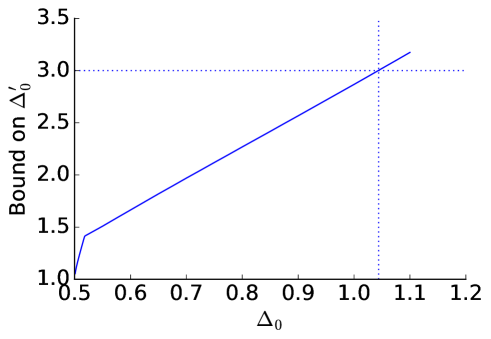
Figure 3: Bounds on the scaling dimensions of the second-lowest neutral scalar operator as a function of $\Delta_{0}$.

We can study the consistency of the four-point function $\langle O_{0}O_{0}O_{0}O_{0}\rangle$ with the crossing symmetry by using the numerical conformal bootstrap program to derive the upper bound on $\Delta_{0}^{\prime}$. Compared to the $\mathbb{Z}_{2}$-odd scalar four-point function studied in El-Showk et al. (2012)El-Showk et al. (2014), the only difference is that we have to additionally require the non-negativity of the linear functional acting on the conformal block coming from $O_{0}$ itself. Although the bounds on $\Delta_{0}^{\prime}$ with $O_{0}$ appearing in the OPE could be weaker than those without $O_{0}$, we found that these two bounds actually coincide (Fig. 3). From this plot we obtain the necessary condition $\Delta_{0}>1.044$ (equivalently, $\nu>0.511$) for the CFTs that contain no singlet relevant scalar operator other than $O_{0}$ so that the corresponding critical point is achieved by tuning only one parameter.

Appendix D Supplementary plots

In this appendix, we present two-dimensional projected plots of the upper bounds on the scaling dimension of the lowest dimensional charge three scalar operator appearing in $O_{1}\times O_{2}$ OPE as a function of $\Delta_{2}$ (for a fixed $\Delta_{1}$). The three-dimensional plot was presented in Fig.2 of the main text. For the range of $\Delta_{2}$, we recall that $1.08<\Delta_{2}<\Delta^{c}_{2}(\Delta_{1})$ must hold from the assumption that all the charge four operators are irrelevant and the bound in Fig.1. When $\Delta_{1}=0.585$, the bound shows a jump as shown in Fig.6.

A similar phenomenon is observed in the fermionic conformal bootstrap analysis Iliesiu et al. (2015). It will be interesting to understand why the scaling dimension 3, corresponding to the marginal value of the deformations, plays a special role in the mixed correlator conformal bootstrap program.

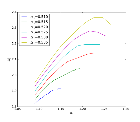
Figure 4: The two-dimensional projection of Fig.2 in the range $\Delta_{1}\leq 0.535$.

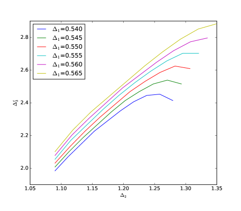
Figure 5: The two-dimensional projection of Fig.2 in the range $0.540\leq\Delta_{1}\leq 0.565$.

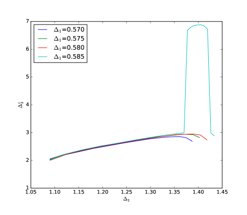
Figure 6: The two-dimensional projection of Fig.2 in the range $0.57\leq\Delta_{1}\leq 0.585$.

References

- Senthil et al. (2004a) T. Senthil, A. Vishwanath, L. Balents, S. Sachdev, and M. P. A. Fisher, Science 303, 1490 (2004a), cond-mat/0311326 .
- Senthil et al. (2004b) T. Senthil, L. Balents, S. Sachdev, A. Vishwanath, and M. P. A. Fisher, Phys. Rev. B 70, 144407 (2004b), cond-mat/0312617 .
- El-Showk et al. (2012) S. El-Showk, M. F. Paulos, D. Poland, S. Rychkov, D. Simmons-Duffin, and A. Vichi, Phys. Rev. D86, 025022 (2012), arXiv:1203.6064 [hep-th] .
- Kos et al. (2014a) F. Kos, D. Poland, and D. Simmons-Duffin, JHEP 06, 091 (2014a), arXiv:1307.6856 [hep-th] .
- El-Showk et al. (2014) S. El-Showk, M. F. Paulos, D. Poland, S. Rychkov, D. Simmons-Duffin, and A. Vichi, J. Stat. Phys. 157, 869 (2014), arXiv:1403.4545 [hep-th] .
- Kos et al. (2014b) F. Kos, D. Poland, and D. Simmons-Duffin, JHEP 11, 109 (2014b), arXiv:1406.4858 [hep-th] .
- Nakayama and Ohtsuki (2014) Y. Nakayama and T. Ohtsuki, Phys. Rev. D89, 126009 (2014), arXiv:1404.0489 [hep-th] .
- Nakayama and Ohtsuki (2015) Y. Nakayama and T. Ohtsuki, Phys. Rev. D91, 021901 (2015), arXiv:1407.6195 [hep-th] .
- Simmons-Duffin (2015) D. Simmons-Duffin, JHEP 06, 174 (2015), arXiv:1502.02033 [hep-th] .
- Kos et al. (2015) F. Kos, D. Poland, D. Simmons-Duffin, and A. Vichi, JHEP 11, 106 (2015), arXiv:1504.07997 [hep-th] .
- Iliesiu et al. (2015) L. Iliesiu, F. Kos, D. Poland, S. S. Pufu, D. Simmons-Duffin, and R. Yacoby, (2015), arXiv:1508.00012 [hep-th] .
- Nakayama (2015) Y. Nakayama, Phys. Rept. 569, 1 (2015), arXiv:1302.0884 [hep-th] .
- Rattazzi et al. (2011) R. Rattazzi, S. Rychkov, and A. Vichi, J. Phys. A44, 035402 (2011), arXiv:1009.5985 [hep-th] .
- Lemos and Liendo (2016) M. Lemos and P. Liendo, JHEP 01, 025 (2016), arXiv:1510.03866 [hep-th] .
- Pelissetto and Vicari (2013) A. Pelissetto and E. Vicari, Phys. Rev. D88, 105018 (2013), arXiv:1309.5446 [hep-lat] .
- Pisarski and Wilczek (1984) R. D. Pisarski and F. Wilczek, Phys. Rev. D29, 338 (1984).
- Aoki et al. (2012) S. Aoki, H. Fukaya, and Y. Taniguchi, Phys. Rev. D86, 114512 (2012), arXiv:1209.2061 [hep-lat] .
- Aoki et al. (2014) S. Aoki, H. Fukaya, and Y. Taniguchi, Proceedings, 31st International Symposium on Lattice Field Theory (Lattice 2013), PoS LATTICE2013, 139 (2014), arXiv:1312.1417 [hep-lat] .
- Kanazawa and Yamamoto (2016) T. Kanazawa and N. Yamamoto, JHEP 01, 141 (2016), arXiv:1508.02416 [hep-th] .
- Halperin et al. (1974) B. I. Halperin, T. C. Lubensky, and S.-k. Ma, Phys. Rev. Lett. 32, 292 (1974).
- Kamal and Murthy (1993) M. Kamal and G. Murthy, Phys. Rev. Lett. 71, 1911 (1993).
- Motrunich and Vishwanath (2004) O. I. Motrunich and A. Vishwanath, Phys. Rev. B 70, 075104 (2004).
- Block et al. (2013) M. S. Block, R. G. Melko, and R. K. Kaul, Physical Review Letters 111, 137202 (2013), arXiv:1307.0519 [cond-mat.str-el] .
- Harada et al. (2013) K. Harada, T. Suzuki, T. Okubo, H. Matsuo, J. Lou, H. Watanabe, S. Todo, and N. Kawashima, Phys. Rev. B 88, 220408 (2013), arXiv:1307.0501 [cond-mat.str-el] .
- Sreejith and Powell (2015) G. J. Sreejith and S. Powell, Phys. Rev. B 92, 184413 (2015).
- Lou et al. (2009) J. Lou, A. W. Sandvik, and N. Kawashima, Phys. Rev. B 80, 180414 (2009), arXiv:0908.0740 [cond-mat.str-el] .
- Metlitski et al. (2008) M. A. Metlitski, M. Hermele, T. Senthil, and M. P. A. Fisher, Phys. Rev. B 78, 214418 (2008), arXiv:0809.2816 [cond-mat.str-el] .
- Campostrini et al. (2006) M. Campostrini, M. Hasenbusch, A. Pelissetto, and E. Vicari, Phys. Rev. B74, 144506 (2006), arXiv:cond-mat/0605083 [cond-mat] .
- Hasenbusch and Vicari (2011) M. Hasenbusch and E. Vicari, Phys. Rev. B 84, 125136 (2011), arXiv:1108.0491 [cond-mat.stat-mech] .
- Carmona et al. (2000) J. M. Carmona, A. Pelissetto, and E. Vicari, Phys. Rev. B61, 15136 (2000), arXiv:cond-mat/9912115 [cond-mat] .
- Xu and Sachdev (2008) C. Xu and S. Sachdev, Phys. Rev. Lett. 100, 137201 (2008).
- Nahum et al. (2015) A. Nahum, P. Serna, J. T. Chalker, M. Ortuno, and A. M. Somoza, Phys. Rev. Lett. 115, 267203 (2015), arXiv:1508.06668 [cond-mat.str-el] .
- Note (1) We thank A. Nahum for discussions. We are informed that D. Simmons-Duffin had made the same observation. It is tantalizing to note, however, that the bound on the singlet operator in symmetric CFTs seems to behave differently at and (i.e. not a straight line) above the kink than at the other (i.e. a straight line).
- Hogervorst et al. (2013) M. Hogervorst, H. Osborn, and S. Rychkov, JHEP 08, 014 (2013), arXiv:1305.1321 [hep-th] .
- Rattazzi et al. (2008) R. Rattazzi, V. S. Rychkov, E. Tonni, and A. Vichi, JHEP 12, 031 (2008), arXiv:0807.0004 [hep-th] .
- The Sage Developers (2015) The Sage Developers, Sage Mathematics Software (Version 6.8.0), http://www.sagemath.org (2015).
- Ohtsuki (2016) T. Ohtsuki, An example of implementation is available at https://github.com/tohtsky/cboot (2016).
- Zinn-Justin (2001) J. Zinn-Justin, RG-2000: Conference on Renormalization Group Theory at the Turn of the Millennium Taxco, Mexico, January 11-15, 1999, Phys. Rept. 344, 159 (2001), arXiv:hep-th/0002136 [hep-th] .
- Lipa et al. (2003) J. A. Lipa, J. A. Nissen, D. A. Stricker, D. R. Swanson, and T. C. P. Chui, Phys. Rev. B68, 174518 (2003).
- Calabrese et al. (2003) P. Calabrese, A. Pelissetto, and E. Vicari, Phys. Rev. B67, 054505 (2003), arXiv:cond-mat/0209580 [cond-mat] .
- De Prato et al. (2003) M. De Prato, A. Pelissetto, and E. Vicari, Phys. Rev. B68, 092403 (2003), arXiv:cond-mat/0302145 [cond-mat] .
- Jiang et al. (2008) F.-J. Jiang, M. Nyfeler, S. Chandrasekharan, and U.-J. Wiese, Journal of Statistical Mechanics: Theory and Experiment 2, 02009 (2008), arXiv:0710.3926 [cond-mat.str-el] .
- Kuklov et al. (2008) A. B. Kuklov, M. Matsumoto, N. V. Prokof’ev, B. V. Svistunov, and M. Troyer, ArXiv e-prints (2008), arXiv:0805.4334 [cond-mat.stat-mech] .
- Sreejith and Powell (2014) G. J. Sreejith and S. Powell, Phys. Rev. B 89, 014404 (2014), arXiv:1311.1444 [cond-mat.stat-mech] .
- Pujari et al. (2013) S. Pujari, K. Damle, and F. Alet, Physical Review Letters 111, 087203 (2013), arXiv:1302.1408 [cond-mat.str-el] .
- Pujari et al. (2015) S. Pujari, F. Alet, and K. Damle, Phys. Rev. B 91, 104411 (2015), arXiv:1502.01035 [cond-mat.str-el] .
- Dyer et al. (2015) E. Dyer, M. Mezei, S. S. Pufu, and S. Sachdev, JHEP 06, 037 (2015), arXiv:1504.00368 [hep-th] .
- Kaul and Sandvik (2012) R. K. Kaul and A. W. Sandvik, Physical Review Letters 108, 137201 (2012), arXiv:1110.4130 [cond-mat.str-el] .
- Murthy and Sachdev (1990) G. Murthy and S. Sachdev, Nuclear Physics B 344, 557 (1990).
- Hermele et al. (2005) M. Hermele, T. Senthil, and M. P. A. Fisher, Phys. Rev. B 72, 104404 (2005).
- Hermele et al. (2008) M. Hermele, Y. Ran, P. A. Lee, and X.-G. Wen, Phys. Rev. B 77, 224413 (2008).
- Pufu (2014) S. S. Pufu, Phys. Rev. D89, 065016 (2014), arXiv:1303.6125 [hep-th] .
- Chester et al. (2015) S. M. Chester, M. Mezei, S. S. Pufu, and I. Yaakov, (2015), arXiv:1511.07108 [hep-th] .
- Chester and Pufu (2016) S. M. Chester and S. S. Pufu, (2016), arXiv:1601.03476 [hep-th] .
- Calabrese et al. (2004) P. Calabrese, P. Parruccini, A. Pelissetto, and E. Vicari, Phys. Rev. B70, 174439 (2004), arXiv:cond-mat/0405667 [cond-mat] .
- Calabrese et al. (2005) P. Calabrese, A. Pelissetto, and E. Vicari, Nucl. Phys. B709, 550 (2005), arXiv:cond-mat/0408130 [cond-mat] .