Predicting dataset popularity for the CMS experiment

Abstract

The CMS experiment at the LHC accelerator at CERN relies on its computing infrastructure to stay at the frontier of High Energy Physics, searching for new phenomena and making discoveries. Even though computing plays a significant role in physics analysis we rarely use its data to predict the system behavior itself. A basic information about computing resources, user activities and site utilization can be really useful for improving the throughput of the system and its management. In this paper, we discuss a first CMS analysis of dataset popularity based on CMS meta-data which can be used as a model for dynamic data placement and provide the foundation of data-driven approach for the CMS computing infrastructure.

1 Introduction

The Large Hadron Collider at Geneva, Switzerland, was designed to uncover mysterious parts of Universe building blocks. The tremendous efforts of physicists all around the globe were rewarded by Higgs discovery through analysis of Run-I data from both ATLAS and CMS experiments [1, 2]. The great success of Run-I was strongly dependent on reliable computing infrastructure. In CMS, the computing model is quite complex. The data collected from the detector are streamed to the HLT farm and organized into trigger streams. Later they are archived at the Tier-0 center at CERN and distributed to CMS Analysis facility (CAF) at CERN and to Tier-1 centers around the globe. Many Tier-2 centers worldwide share a portion of the data for further processing and Monte-Carlo generation. Finally, the Tier-3 centers (mostly at University levels) are used for various analysis tasks. Such distributed Computing Model is demonstrated to be reliable and flexible enough during Run-I operations, see [3].

During Run-I, CMS collected and processed more than 10B data events and simulated more than 15B events. The data transfer throughput peaks at few PB per week placing the data across hundreds of GRID sites for various user activities, ranging from data operations tasks to individual physics analysis. Even though CMS is able to successfully handle the data through Run-I operations [4] the experiment is looking at different ways to improve the system and reduce its operation cost and manual labor.

In this paper, we present a first attempt to understand different aspects of the CMS dataset popularity by the analysis of the CMS computing model. We start with the problem statement in Section 2, followed by discussions of various streams of information at our disposal from CMS data management systems. Section 3 provides a description of the architecture and implementation of different components used by Machine Learning (ML) algorithms to model and predict CMS dataset popularity. In particular, we discuss time series (referred to as “rolling”) analysis for future predictions, operational cost of results obtained by ML algorithms and seasonality aspect of the data.

2 Problem statement

The CMS dataset popularity is a metric that quantifies user activities in CMS [5]. The data produced by the detector are logically organized into hierarchical structure, such as runs, files, blocks and datasets. The data coming from the detector are grouped into runs which represent a unit of the data-taking process. These runs are stored into files which are suitable for data processing by reconstruction or analysis programs. The files themselves are grouped into blocks which are used by data operations teams as atomic units for data transferring among the sites. Blocks are grouped into datasets which represent a processing chain of specific physics processes. Once data is produced and become available for end-users they use datasets as a common unit to submit their processing or analysis jobs. Every job will resolve a given dataset into series of files and process them at once. The outcome will be either stored in other files and a new dataset will be formed or it can be converted into n-tuples, histograms or any other form used by physicists in their analysis. Therefore it is possible to measure user activities in terms of dataset popularity, i.e. those datasets which are used in analysis jobs more often than others can be considered as popular.

During Run-I we collected more than 1TB of meta-data stored in various databases. More than 400K datasets, 4.5M blocks and 100M files were recorded in data bookkeeping system (DBS), see [4]. Only a portion of these datasets were actively accessed by end-users. The other parts were transferred once and had a very low access rate. The latter can lead to sub-optimal utilization of CMS storage space as well as overhead in the data management system with unnecessary data transfers. On the other hand, the reduction of dataset access latencies can be very useful for load balancing and scheduling jobs among the sites. This becomes especially important during rush periods when results are prepared for major events such as conferences. Therefore it is desirable to understand the nature of CMS dataset popularity in order to improve our computing model and reduce its operational cost. Among different possibilities to tackle these issues we decided to model and predict CMS dataset popularity via ML algorithms based on historical usage of datasets via various meta-data information available to us.

The CMS data management system is composed by several systems [4, 5]: PhEDEx (dataset replication system), DBS (data bookkeeping catalog), Dashboard (global monitoring system which keeps tracks of user jobs), SiteDB (site and user database), PopDB (CMS datasets popularity database), DDM (Dynamic Data Management system) and others. The PopDB database keeps historical information of datasets usage in various metrics, e.g. number of total and user accesses per dataset, as well as total CPU time spent on each datasets during processing or analysis jobs. This information is used by DDM to replicate popular datasets to other sites. But the latter happens post-factum and requires sufficient amount of historical data to be accumulated up-front to trigger the replication process. To fill this gap we proposed to investigate a possibility to predict CMS dataset popularity based on existing meta-data for newly created datasets and use these predictions as a seeding mechanism for DDM machinery.

3 Architecture & Implementation

We started with evaluation of CMS data services and their underlying back-ends as a possible sources of information for CMS dataset popularity problem. We divided them into three categories: structured data which can be obtained from CMS data-services such as DBS, PhEDEx, Dashboard, SiteDB, PopDB; the semi-structured data which can be found from CMS web logs, calendar systems and un-structured data, such as HyperNews forums, CMS twikies, etc. Obviously obtaining information from structured and semi-structured sources is much easier than un-structured ones. The latter will require significant pre-processing effort which is far beyond our abilities at the moment. Therefore, we concentrate our work only on first source of information, i.e. structured data extracted from CMS data-services.

Figure 1: Flow diagram of DCAFPilot framework which collects and pre-processes information from various CMS data-services, anonymizes information within internal cache and passes them on to underlying ML algorithms.

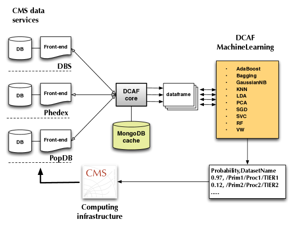
We developed DCAFPilot (Data and Computing Analysis Framework Pilot) [7] framework in order to understand the metrics, the analysis workflow and the necessary tools (with possible technology choices) needed to tackle this problem. Its overall architecture is shown in Figure 1. It collects information from various CMS data-services, passes it to a pre-processing step which ensures that information stays anonymous and later to external ML algorithms for model building. The predictions are represented in a form of probabilities and dataset names which later can be fed back into the CMS computing infrastructure, e.g. used by DDM system as initial seeds for dataset replication.

The DCAFPilot framework was implemented in python and integrated with the scikit-learn ML library [8]. We also supplement it by Yahoo Vowal Wabbit [9] and Distributed Gradient Boosting xgboost ML libraries [10]. As a baseline we used five algorithms: RandomForest [11], LinearSVC [12], SGDClassifier [13], VW [9], and xgboost [10] to establish automated machinery to build and train the model, predict CMS dataset popularity in up-coming week and understand the cost of the modeling procedure.

3.1 Data collection

We used five CMS data-services (DBS, PhEDEx, SiteDB, Dashboard, PopDB) to collect all required meta-data information suitable for ML analysis. In addition, the DBS services consists of four different instances used to publish globally accessible datasets and physics analysis ones and we used all of them during data collection phase. The data from CMS services were available via data-service APIs. In total, we utilized about a dozen of APIs from aforementioned CMS data-services, places 800K queries about 200K datasets, 900 software releases, 500 site entries and 5K user entries. The obtained data were stored in an internal cache, see Figure 1, and anonymized either by using internal database ids or via internal hash function. The data collection procedure was automated via UNIX cronjobs. The data were organized by weeks with total of 52 data files per year, where each file has 82 attributes. The datasets were extracted from PopDB and complemented by datasets from the DBS system. The former datasets were used to define dataset popularity metric, while latter ones represented “unpopular” data. One year of data was roughly translated into the 82$\times$600000 dataframe. In total, we collected 130 dataframe files (52 files per year), worth of $\sim 1.5$M measurements for different CMS datasets spawning over the years 2013-2015. Separately, we also generated conference count dataframe based on the CMS CINCO [14] database. It contains counters for up-coming conferences where CMS presents its results. The counters collect total number of conferences in 1,2,4,6,10 weeks followed by 5 week intervals up-to 70 weeks in the future. This dataframe was used as a complement to dataset meta-data to study the influence of conferences on the CMS dataset popularity (see Section 3.6 for discussion).

The collected data presents a good representation of various user activities through 2013-2015 years. These years cover Run-I era, preparation for Run-II and future detector upgrade studies. And, we expects that such activities will only grow through the Run-II phase and beyond.

3.2 Dataset popularity

Our first task was to define dataset popularity metric. As simple as it sounds it had many dimensions. The popularity DB provides us six different metrics: the number of accesses to a given dataset, the number of users/day recorded for a dataset, the total number of CPU hours spent on a given dataset, along with normalized values of those attributes over full number of datasets.

Figure 2: Number of accesses per dataset and sub-set of available attributes in a correlation plot for the 2013-2015 data sets.

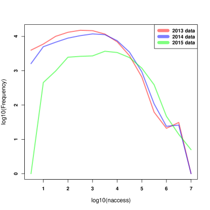
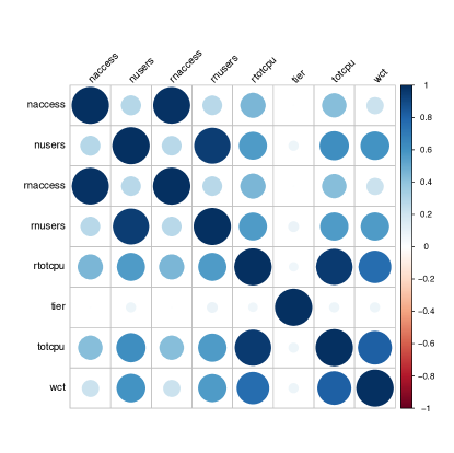
Figure 2 shows the behavior of some metrics recorded in popularity DB. Even though the shape of distributions of different years looks alike, we found that data themselves required further clean-up and understanding. For instance, number of users at low access patterns had gaps which represent the fact that our users were picky about certain datasets. The overall value of different metrics in 2015 were lower with respect to 2013/2014 years which reflects the usage of 2015 data sample (we only used half of the year available at the time of our studies). And, we have significant correlations among some attributes, e.g. number of dataset accesses is highly correlated with number of users used those datasets in their jobs, see Figure 2.

In addition, we were dealing with datasets composed out of 59 different data tiers within our sample. Each data-tier represents a specific interests within physics community, e.g. the raw data, processing data, the analysis data etc. The further work was only concentrated on five different data-tiers: AOD - Analysis Object Data, AODSIM - AOD with simulated information, MINIAOD - reduced AOD objects, MINIAODSIM - MINIAOD with simulated information and USER data-tier to denote user-based datasets. These five data-tiers represent the main interests for dataset popularity since they correspond mostly to main user activities, such as analysis and data-processing, rather than daily activities of various data operations teams within the CMS experiment. The latter can be considered as “routine” tasks and obviously are well-defined within the experiment.

Table 1: Effects of applied cuts on the different data tiers.

Data tier/Cut	No cut	naccess$>$10	log(nuser)$>$2
AOD	4924 (7.25%)	4687 (8%)	1285 (35%)
AODSIM	21090 (31%)	18825 (32%)	1547 (42%)
MINIAOD	7 (0.01%)	6 (0.01%)	0
MINIAODSIM	1083 (1.5%)	792 (1.3%)	28 (0.8%)
USER	34127 (50%)	28777 (49%)	380 (10%)
ALL	67892	59222	3683

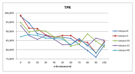
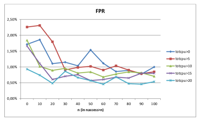
We collected the data for 2013, 2014 and first half of 2015 data and analyzed data-tiers breakdown within these samples. Table 1 shows the total number of datasets recorded in PopDB along with cuts for different data-tiers within 2014 dataframe. Further, we performed analysis of various cuts based on yield of TP (true positive), FP (false positive), TN (true negative) and FN (false negative) rates using Random Forest classifier. The Figure 3 shows model behavior under different $naccess$ and $totcpu$ cuts. Based on this studies we found that $naccess>10$ and $totcpu>10$ or $naccess>10$ cuts provide the most the most promising TP/FP/TN/FN rates. For further studies we opted for simple threshold, $naccess>10$.

Figure 3: True positive and False positive rates for different values of $naccess$ and $totcpu$ parameters using Random Forest classifier over 2014 datasets.

3.3 Workflow

Our workflow was organized in the following way. The data was collected on a weekly basis via periodic cronjob which requested dataset information from PopDB for a given week. For every dataset in this set we obtained meta-data information from DBS, PhEDEx, SiteDB and Dashboard systems. This data was complemented by using random datasets from DBS system. The average time to collect 1 week of data took several hours and fade out gradually upon filling out internal cache. It was possible to run these jobs within single VM without requiring for additional resources. As mentioned in Section 3.1 we added to each dataframe the “unpopular” datasets meta-data with 1:10 ratio. This ratio was used to supplement signal data from PopDB with noise one from DBS system, i.e. we used random datasets from DBS which had no records in PopDB for given time period. All data attributes were anonymized via internal cache hashing mechanism and checked for correlations. Even though we were able to get 82 attributes representing each dataset we dropped 12 attributes due to their bias towards the popularity metric. We used additional transformation step to convert obtained dataframes into classification problem, for which we used a cut discussed in Section 3.2. At this step the data were ready to be fed into any ML library.

3.4 Processing

Once the data were transformed into suitable format for ML we used the “rolling” approach which consists of the following steps:

• obtain a set of data up to the week in question (usually we kept one year worth of data) and train a specific classifier;

• obtain new data and make a prediction for selected data-tiers (we are only interested in user based data and AOD datasets);

• use the prediction as a seeding for DDM service who allocates replicas of popular dataset at various sites;

• once data for the week in question becomes available in PopDB, compare the predictions to the actual dataset access patterns. This step can be used to adjust the model in the future.

The former two steps were performed with five ML classifiers: RandomForest, LinearSVC, SGDClassifier, VW and xgboost (see Section 3), and standard 70/30 split was used to test the model via cross-validation. We measured the outcome of True Positive (TP), True Negative (TN) rates for different data-tiers and estimated the operational cost of False Positive (FP) and False Negative (FN) rates. In the following, the results obtained from these studies are presented; the last two steps in the previous list are under implementation in the production system.

3.5 Classification results

We used 2013 data sample as the initial dataframe and gradually added weekly data to measure TP/TN/FP/FN rates for data through 2014. Among all used classifiers we found that SGDClassifier performs best, giving less than 10% error for TP/TN rates for the majority of the weeks.

From the results of various classifiers we found that prediction errors are larger during “vacation” periods, i.e. first and last weeks of the year, when CMS users are less active. During normal operation during the year all classifiers shown that it was feasible to keep TP/TN error below 10-15% using their default parameters. The fine tuning of algorithms were not performed since we mostly concentrated on setting up machinery for our task. The large deviations of errors were caused by different sensitivity of underlying algorithm to specific data tiers. Some data tiers, e.g. MINIAOD, were introduced during 2014 and did not gain too much access pattern among our users and therefore had larger errors. While others, e.g. AOD, AODSIM, and USER, had smaller errors throughout the entire year. Table 2 summarizes the mean and standard deviations for different statistics metrics grouped by data-tiers.

We found that only AOD, AODSIM and USER data-tiers gave reasonable predictions and their errors are stable through the entire year. The MINIAOD and MINIAODSIM datasets were less sensitive to algorithm due to the fact that they only become available for end-user through 2014 and did not attract user interest. In fact, they represented only 1.5% of entire data sample used in this analysis.

Table 2: Summary of TPR (true positive rate, i.e. sensitivity), TNR (true negative rate, i.e. specificity), FP (false positive) and FN (false negative) values for different data tiers.

Data tier	TPR	TNR	FP	FN
AOD	0.97$\pm$0.05	0.99$\pm$0.02	0.005$\pm$0.011	0.015$\pm$0.029
AODSIM	0.93$\pm$0.13	0.99$\pm$0.02	0.008$\pm$0.016	0.021$\pm$0.045
MINIAOD	0.11$\pm$0.32	0.99$\pm$0.02	0.014$\pm$0.026	0.001$\pm$0.007
MINIAODSIM	0.49$\pm$0.48	0.99$\pm$0.02	0.009$\pm$0.016	0.007$\pm$0.031
USER	0.93$\pm$0.15	0.98$\pm$0.02	0.014$\pm$0.021	0.011$\pm$0.023

The obtained errors on FP rates can be easily translated into data-transfer and extra disk space overhead we may face. For example, an average size of CMS dataset is around 2TB. If we have 1% of FP rate, see Table 2, and take on average 500 datasets created in CMS this will translate into extra 10TB of data-transfer per week out of few PB of data transfer CMS is doing on weekly basis. Therefore the overhead would be $\sim 1\%$ of total transfer rate. Such overhead can be easily accounted by data transfer team. We found that the cost of FN rate can be considered as “irrelevant” from operational point of view since it will correspond to current mode of operations in CMS, since data placement is done manually via current snapshot of site occupancy. But in the ideal world where computing resources will be driven by such data popularity predictions the FN rate will translate into longer latencies of analysis user jobs. On average we have 1.5M jobs submitted every day. The 1% of FN rate will correspond that $\sim 15$K jobs will compete for resources of a site where popular dataset may resides. On another hand, the data driven approach would reduced overhead of site utilization. So far, our sites are populated with data which we put over there rather the data which will become popular. For example, we found that majority of datasets are accessed only by a few users. Therefore a better data placement will directly translate into site utilization savings, further studies of which are underway.

3.6 Prediction from information beyond dataset features

Even though we used historical information to predict popularity of datasets in a future we also considered that future events, such as up-coming conferences, group meetings and discussion within various physics groups can stimulate access patterns to certain datasets. Such studies will require data-mining of user based discussion groups, meetings agendas and up-comping conferences. As a starting point we used the CINCO CMS conference database [14] where physics conferences are registered and physicists are assigned to present their work on physics analysis.

Naively, we thought that some datasets which represent certain physics channels may become popular before up-coming conferences where physicist present their results. To test this idea we evaluated if the future conference weekly counts - if used together with the features of the datasets - could improve the classification of whether a dataset is popular or unpopular, with respect to using only the features of the dataset. This was done by comparing the classification accuracies, comparing the feature importance scores given by random forest classifiers for individual features, and comparing the p-values of the $\chi^{2}$-independence test and the ANOVA F test between individual features and the popularity outcome. The experiment has not shown improvement yet, in part because the classification performance was already nearly perfect for the limited time period when the conference data was available. This also lead us to explore the influence of the conference data from alternative perspectives.

For instance, we calculated the cross correlation between the weekly count time series of conferences and the one of the accesses to each dataset at different time lags, and found that the time lag at which the cross correlation peaks is roughly 75 weeks for most datasets. We also found that for some datasets cross correlation is peaking at a positive lag implying that future conference schedules can affect the current dataset access, while for others it peaks at a negative lag meaning that past conferences can still have residual influence on the current dataset access. Figure 4 shows that such lags have significant cross correlations.

Figure 4: Histograms of lags with maximum cross correlation (see text for more details).

Finally, we tried to find out if each time series contains significant seasonality, i.e. periodicity. This was done by calculating the Discrete Fourier Transform (DFT) on the time series using the Fast-Fourier Transform (FFT) algorithm and searched for the most significant spike that represents the frequency of seasonality. We found a yearly seasonality effect for the conferences, a shorter-period seasonality for some datasets (for example, 15-week period), and no seasonality for other datasets (see Figure 5).

Figure 5: Seasonality effect of random datasets from 2014 data sample. Both plots show DFT of access count per week time series of a dataset. The length of time series is 116 weeks. The highest spike of top plot for dataset ID=471188 occurs at the 8-th frequency and corresponds to a time period of 116/8 = 15 weeks. The DFT plot of another dataset ID=701364 does not show seasonality in the dataset access series.

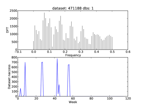
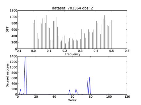
These studies demonstrate that the conference count and some CMS datasets access counts can show some seasonality, and there is significant correlation between conference count and most dataset access counts. But further studies are required to see if such observations can improve the overall prediction for dataset popularity, and it is especially interesting in the context of specific data-tiers.

4 Summary

The results of this pilot project provides a solid foundation and a working pilot framework for future R&D work on data mining of several aspects of the CMS computing model. We demonstrated that we are able to successfully predict CMS dataset popularity based on collected CMS meta-data. The obtained results shows that small FP/FN rates are possible to achieve and can be interpreted as overhead in data-transfer and job latencies. We estimated that obtained FP rate can introduce only 1% overhead to existing data transfer rate and can be easily managed by operational team. The small FN rate can lead to better sites utilization and provide operational savings in the long term. We are evaluating to turn this pilot project into production and use dataset popularity predictions as initial seeding for the DDM [5] system. In addition, we are interested in further investigations of seasonality effects for specific data tiers. The relatively small errors for the few discussed data-tiers can be turned into better data placement and reduced latencies of analysis jobs during first week of data appearance. This will lead to better analysis throughput and user satisfaction with their data processing needs, more awareness in dynamic data placement tactics across different sites, as well as better usage of site resources in the CMS GRID infrastructure.

References

- [1] ATLAS experiment, Observation of a new particle in the search for the Standard Model Higgs boson with the ATLAS detector at the LHC, Physics Letters B, Volume 716, Issue 1, pp 1-29, 2012.
- [2] CMS experiment, Observation of a new boson at a mass of 125 GeV with the CMS experiment at the LHC, Physics Letters B, Volume 716, Issue 1, pp 30-61, 2012.
- [3] J. Adelman et al, CMS Computing Operations during Run 1, Journal of Physics: Conference Series 513 (2014) 032040.
- [4] M. Giffels, Y. Guo, V. Kuznetsov, N. Magini and T. Wildish The CMS Data Management System J. Phys.: Conf. Ser. 513 042052 doi:10.1088/1742-6596/513/4/042052
- [5] F.H. Barrerio Megino et al, Implementing data placement strategies for the CMS experiment based on a popularity model J. Phys.: Conf. Ser. 396 032047 doi:10.1088/1742-6596/396/3/032047
- [6] V. Kuznetsov, T. Wildish, L. Giommi, D. Bonacorsi Exploring patterns and correlations in CMS Computing operations data with Big Data analytics techniques International Symposium on Grids and Clouds (ISGC) 2015, Academia Sinica, Taipei, Taiwan
- [7] https://github.com/dmwm/DMWMAnalytics/
- [8] http://scikit-learn.org/stable/
- [9] https://github.com/JohnLangford/vowpal_wabbit/wiki
- [10] https://github.com/dmlc/xgboost
- [11] L. Breiman, Random Forests, Machine Learning 45 (1) 5–32. doi:10.1023/A:1010933404324
- [12] C. Cortes, V. Vapnik, Support-vector networks, Machine Learning, 20, 273-297 (1995),
- [13] Stochastic Gradient Descent, Website, 2010. http://leon.bottou.org/projects/sgd
- [14] Cms INformation on COnferences (CINCO) data-service, https://cms-mgt-conferences.web.cern.ch/