Modal analysis of gravitational instabilities in nearly Keplerian, counter-rotating collisionless discs

Abstract

We present a modal analysis of instabilities of counter-rotating, self-gravitating collisionless stellar discs, using the recently introduced modified WKB formulation of spiral density waves for collisionless systems (Gulati & Saini). The discs are assumed to be axisymmetric and in coplanar orbits around a massive object at the common center of the discs. The mass in both discs is assumed to be much smaller than the mass of the central object. For each disc, the disc particles are assumed to be in near circular orbits. The two discs are coupled to each other gravitationally. The perturbed dynamics of the discs evolves on the order of the precession time scale of the discs, which is much longer than the Keplerian time scale. We present results for the azimuthal wave number $m=1$ and $m=2$, for the full range of disc mass ratio between the prograde and retrograde discs. The eigenspectra are in general complex, therefore all eigenmodes are unstable. Eigenfunctions are radially more compact for $m=1$ as compared to $m=2$. Pattern speed of eigenmodes is always prograde with respect to the more massive disc. The growth rate of unstable modes increases with increasing mass fraction in the retrograde disc, and decreases with $m$; therefore $m=1$ instability is likely to play the dominant role in the dynamics of such systems.

1 Introduction

Observations of galactic nuclei are limited by the resolution of present day telescopes. Of the few galaxies for which such observations are available, double peak stellar distribution has been observed in galaxies M$31$, a spiral galaxy, and NGC$4486$B, which is an elliptical galaxy at the center of virgo cluster (Lauer et al., 1993, 1996). Distribution of stellar peaks in both these galaxies differ from each other: the peaks in NGC$4486$B are symmetric w.r.t. the photo-centre in contrast to the off–centre peaks in M$31$. Motivated by the work of Touma (2002), Sambhus & Sridhar (2002) proposed that unstable eccentric modes due the presence of counter–rotating streams of matter could be present in the nuclei of galaxy M$31$ giving rise to eccentric discs. Counter-rotating streams of matter could form possibly due to accretion of stars from in-falling globular clusters. Such eccentric discs are thought to be the reason behind observed lopsided multiple–peaked brightness distribution around its nuclear black hole, as was proposed by Tremaine (1995) for M$31$. However, the double-peak stellar distribution in NGC$4486$B, being more symmetrical around the photo-centre, is plausibly due to $m=2$ ($m$ being the azimuthal quantum number) unstable modes than $m=1$ eccentric modes for M$31$ (Tremaine, 2001; Sambhus & Sridhar, 2002; Gulati et al., 2012).

Unstable eccentric modes are known to exist in self-gravitating counter–rotating streams of matter (Zang & Hohl, 1978; Araki, 1987; Sawamura, 1988; Merritt & Stiavelli, 1990; Palmer & Papaloizou, 1990; Sellwood & Merritt, 1994; Lovelace et al., 1997; Touma, 2002; Sridhar & Saini, 2010; Gulati et al., 2012). Specifically, the counter-rotating discs in the systems discussed above happen to be dominated by the influence of a central black hole, thereby making them nearly Keplerian. Moreover, mainly comprising stars, these discs are collisionless. Earlier studies of nearly Keplerian counter–rotating discs either modelled the disc(s) using a system of rings (Touma, 2002), or restricted themselves to softened gravity fluid discs (Sridhar & Saini, 2010; Gulati et al., 2012)—which notably supports only $m=1$ modes—or some similar system. The fluid analysis is inadequate to describe systems comprising stellar discs, especially for $m>1$; since using the WKB analysis Jalali & Tremaine (2012) showed that slow modes with $m>1$ exist for nearly Keplerian collisionless discs. These form a new class of modes, which have hitherto not been explored in detail.

Recently, Gulati & Saini (2016) (Paper I hereafter) have formulated an integral-eigenvalue equation for collisionless self-gravitating disc in the epicyclic approximation using a modified WKB formulation. In the present paper we apply this formalism to two coplanar counter-rotating discs. The disc profiles considered in this work are the same as in Paper I. Both discs interact with each other only through gravity. We consider the discs in the external potential of a central black hole and treat them to be nearly Keplerian systems. Such systems have been shown to support Slow modes that are much slower in comparison to the Keplerian flow of the disc. In this work we investigate the properties of these modes as a function of mass fraction in retrograde disc and the azimuthal wave number $m$.

In the next section we introduce the system of unperturbed discs. Thereafter, in § 3 we derive the integral equation for two nearly Keplerian counter-rotating discs. Next, we take the slow mode limit to derive the integral eigenvalue equation in § 4, where we show that all $m$ modes are unstable if the mass in retrograde disc is non-zero. We also discuss the general properties of the these unstable modes. In § 5, we discuss the details of our numerical method, and in §-6 we discuss the numerical results for different values of mass fraction in the retrograde disc. We conclude in § 7.

2 Unperturbed discs

We begin by approximating our discs to be razor thin, i.e., we restrict ourselves to $z=0$ plane, and use polar-coordinates $\mathbf{r}\equiv(R\,,\phi)$ in the plane of the discs, with the origin at the location of the central mass. The unperturbed disc is a superposition of two coplanar collisionless counter-rotating discs where the disc particles interact with each other gravitationally through Newtonian gravity. Throughout this paper, the superscripts ‘$+$’ and ‘$-$’ refer to the prograde and the retrograde discs, respectively.

The unperturbed potential, $\Phi_{0}(R)$, is the sum of Keplerian potential due to the central mass and the self-gravity of both ‘$\pm$’ discs:

$$\Phi_{0}(R) \;=\;-\frac{GM}{R}+\Phi_{\rm d}(R)\,,$$ (1)

$$\Phi_{\rm d}({\bf{r}}) \;=\;-G\int\frac{\Sigma_{{\rm{d}}}^{{\scriptscriptstyle{+}}}({\bf{r^{\prime}}})+\Sigma_{{\rm{d}}}^{{\scriptscriptstyle{-}}}({\bf{r^{\prime}}})}{|{\bf{r}}-{\bf{r^{\prime}}}|}\mbox{${\mathrm{d}}$}^{2}r^{\prime}\,.$$ (2)

In this paper we are interested in studying the discs for which $M_{{\rm{d}}}/M\equiv\varepsilon\ll 1$, where $M_{{\rm{d}}}$ is the total mass of the disc and $M$ is the central mass. The disc potential $\Phi_{\rm d}$ is then on the order $\mathnormal{O}(\varepsilon)$ smaller in comparison to the Keplerian potential due to the central mass. Azimuthal and radial frequencies ($\pm\Omega$ and $\pm\kappa$, respectively) for both ‘$\pm$’ discs are given by

$$\Omega^{2}(R) \;=\;\frac{GM}{R^{3}}+\frac{1}{R}\frac{\mbox{${\mathrm{d}}$}{\Phi_{\rm d}}}{\mbox{${\mathrm{d}}$}{R}}\,,$$ (3)

$$\kappa^{2}(R) \;=\;\frac{GM}{R^{3}}+\frac{3}{R}\frac{\mbox{${\mathrm{d}}$}{\Phi_{\rm d}}}{\mbox{${\mathrm{d}}$}{R}}+\frac{\mbox{${\mathrm{d}}$}\,^{2}{\Phi_{\rm d}}}{\mbox{${\mathrm{d}}$}{R}^{2}}\,.$$ (4)

The precession rate $\pm\dot{\varpi}$ for such near circular orbits is

$$\dot{\varpi}(R) \;=\;\Omega(R)-\kappa(R)$$

$$\;=\;-\frac{1}{2\Omega(R)}\left(\frac{2}{R}\frac{\mbox{${\mathrm{d}}$}{}}{\mbox{${\mathrm{d}}$}{R}}+\frac{\mbox{${\mathrm{d}}$}\,^{2}{}}{\mbox{${\mathrm{d}}$}{R}^{2}}\right)\Phi_{{\rm{d}}}(R)+\mathnormal{O}(\varepsilon^{2})\,.$$ (5)

In the expression for $\dot{\varpi}$ we have retained terms up to linear order in $\varepsilon$. For nearly Keplerian discs $\varepsilon\ll 1$; and the slow modes in such disc exist due to this small non-zero precession, and the complex eigenfrequencies of modes is on the same order as $\dot{\varpi}$.

The disc particles in both prograde and retrograde discs are assumed to be in nearly circular orbits, called epicyclic orbits (Binney & Tremaine, 2008). We note that $(R^{\prime},v_{R}^{\prime})$ are the same for the ‘$\pm$’ discs, whereas the sense of rotation, whether prograde or retrograde, does change the expressions for $(\phi^{\prime},{\tilde{v}}_{\phi}^{\prime})$ for the respective discs. The phase-space coordinates of particles for both $\pm$ discs are given by

$$R^{\prime\pm} \,=\,R+\frac{\gamma{\tilde{v}}_{\phi}}{\kappa}\left(1-\cos(\tau)\right)+\frac{v_{R}}{\kappa}\sin(\tau)\,,$$

$$\phi^{\prime\pm}\,=\,\phi\pm\frac{\Omega\tau}{\kappa} \pm\frac{\gamma\gamma^{\prime}}{2\kappa}{\tilde{v}}_{\phi}\tau\pm\frac{\gamma}{R\kappa}\left[\gamma{\tilde{v}}_{\phi}\sin(\tau)-v_{R}\left(1-\cos(\tau)\right)\right]\,,$$ (6)

and

$$v_{R}^{\prime\pm} \,=\,v_{R}\cos(\tau)+\gamma{\tilde{v}}_{\phi}\sin(\tau)\,,$$

$$\gamma{\tilde{v}}_{\phi}^{\prime\pm} \,=\,\pm\left(\gamma{\tilde{v}}_{\phi}\cos(\tau)-v_{R}\sin(\tau)\right)\,,$$ (7)

where at time $t^{\prime}=t$, the phase-space coordinates $({\bf{r^{\prime}}},{\bf{v^{\prime}}})=({\bf{r}},{\bf{v}})$. Also ${\tilde{v}}_{\phi}(R)=v_{\phi}(R)-v_{c}(R)$;  $v_{c}(R)=R\,\Omega(R)$;  $\gamma(R)\;=\;2\Omega(R)/\kappa(R)$;  $\tau\,=\,\kappa_{g}(t^{\prime}-t)$;  $\kappa_{g}\;=\;\kappa(R_{g})$ where $R_{g}$ is the mean radius of the orbit for a given angular momentum; and $\gamma^{\prime}$ is the derivative of $\gamma$ w.r.t. $R$.

The two discs are treated as collisionless and are descried by the Collisionless Boltzmann equation (CBE). A solution of CBE in the $z=0$ plane under the epicyclic approximation for axisymmetric stellar discs is given by the Schwarzschild Distribution Function (DF) (Binney & Tremaine, 2008), which for $\pm$ disc is given by

$$f_{0}^{\pm}(R^{\pm},v_{R}^{\pm},{\tilde{v}}_{\phi}^{\pm})\;=\;\frac{\gamma\Sigma_{{\rm{d}}}^{\pm}(R)}{2\pi\sigma_{R}^{\pm^{2}}}\exp\left(-\,\frac{v_{R}^{\pm^{2}}+\gamma^{2}{\tilde{v}}_{\phi}^{\pm^{2}}}{2\sigma_{R}^{\pm^{2}}}\right)\,,$$ (8)

where $\Sigma_{{\rm{d}}}^{\pm}(R)$ and $\sigma_{R}^{\pm}(R)$ are the unperturbed surface density profile and the radial component of the velocity dispersion, respectively. Note that $\gamma$ is same for both ‘$\pm$’ discs.

3 Perturbed disc: Integral equation for two counter-rotating discs

We wish to study the evolution of the discs described above in the linear perturbation regime. We begin by perturbing the initial DF’s, $f_{0}^{\pm}$, such that

$$f^{\pm}(R,\phi,v_{R},{\tilde{v}}_{\phi},t)=f_{0}^{\pm}(R,v_{R},{\tilde{v}}_{\phi})+f_{1}^{\pm}(R,\phi,v_{R},{\tilde{v}}_{\phi},t)\,.$$ (9)

The perturbation $f_{1}^{\pm}$ are assumed to be $\sim\varepsilon f_{0}$ and henceforth we shall retain terms only up to linear order in the perturbed quantities. Volume integral of $f_{1}^{\pm}$ over velocity space gives the perturbed surface density $\Sigma_{1}^{\pm}$, i.e. ,

$$\Sigma_{1}^{\pm}(R,\phi,t)=\int f_{1}^{\pm}(R,\phi,v_{R},{\tilde{v}}_{\phi},t)\mbox{${\mathrm{d}}$}^{2}{\bf{v}}\,,$$ (10)

where $\mbox{${\mathrm{d}}$}^{2}{\bf{v}}=\mbox{${\mathrm{d}}$}v_{R}\mbox{${\mathrm{d}}$}{\tilde{v}}_{\phi}$. Perturbations in the surface density gives rise to perturbed potential, which can be calculated using the Poisson integral (see Paper I). The total gravitational potential at any $(R,\phi,t)$ is a linear sum of the potential due to the prograde and the retrograde discs. We linearise the CBE for both ‘$\pm$’ discs to get

$$\frac{\mbox{${\mathrm{d}}$}{f_{1}^{\pm}}}{\mbox{${\mathrm{d}}$}{t}}=-\left[f_{0}^{\pm},\Phi_{1}\right]\,,$$ (11)

where the time derivative on the left hand side is taken along the unperturbed orbit, and the bracket $[*,*]$ on the right hand side is the Poisson Bracket. We solve these equation for the prograde and the retrograde discs separately for epicyclic orbits as in Paper I to get

$$\Sigma_{a}^{\pm}(R)= \,\frac{2G\Sigma_{d}^{\pm}}{R^{5/2}\kappa^{2}}\sum_{n=1}^{\infty}\left(\frac{n^{2}}{n^{2}-s^{\pm^{2}}}\right)\int_{-\infty}^{\infty}\frac{\mbox{${\mathrm{d}}$}\alpha}{2\pi}\,N(\alpha,m)A_{m}(\alpha)\,{\rm e}^{{\rm i}\alpha q}\,B_{n}(\alpha,\chi^{\pm})\,,$$ (12)

where $q=\ln R$, $s^{\pm}=(\omega\mp m\Omega)/(\pm\kappa$), $\chi=\sigma_{R}^{\pm^{2}}\alpha^{2}/R^{2}\kappa^{2}$, $\omega$ is the temporal eigenfrequency, and

$$A_{m}(\alpha) \,=\,\int_{-\infty}^{\infty}\mbox{${\mathrm{d}}$}q^{\prime}\,R^{\prime 3/2}\left[\Sigma_{a}^{+}(R^{\prime})+\Sigma_{a}^{-}(R^{\prime})\right]{\rm e}^{-{\rm i}\alpha q^{\prime}}\,,$$ (13)

$$N(\alpha,m) \,=\,\pi\frac{\displaystyle{\Gamma\left(\frac{m}{2}+\frac{1}{4}+\frac{{\rm i}\alpha}{2}\right)\Gamma\left(\frac{m}{2}+\frac{1}{4}-\frac{{\rm i}\alpha}{2}\right)}}{\displaystyle{\Gamma\left(\frac{m}{2}+\frac{3}{4}+\frac{{\rm i}\alpha}{2}\right)\Gamma\left(\frac{m}{2}+\frac{3}{4}-\frac{{\rm i}\alpha}{2}\right)}}\,,$$ (14)

$$B_{n}(\alpha,\chi^{\pm} )\,=\,\frac{\alpha^{2}}{\chi^{\pm}}\,\,{\rm e}^{-\chi^{\pm}}\,I_{n}(\chi^{\pm})\,.$$ (15)

For mathematical details we refer the reader to Paper I. Note that $N(\alpha,m)$ and $B_{n}(\alpha,\chi^{\pm})$ are real and even functions of $m$ and $\alpha$ both. $I_{n}(x)$ is the modified Bessel’s function of integer order $n$ and $\Gamma(x)$ is the Gamma function for a complex argument $x$. From eqn. (12) it can be easily verified that the equations are symmetric under the simultaneous transformations $\{$‘$+$’, $\omega\}$ $\to$ $\{$‘$-$’, $-\omega\}$, which simply interchanges the meaning of prograde and retrograde discs.

4 Integral eigenvalue equation for Slow modes

The presence of an infinite series in the integral equation eqn. (12), makes it difficult to solve it in its present form. As explained in $\S~{}\ref{unprtbd_dsc}$, the presence of a small precession in nearly Keplerian discs allows for the existence of slow modes in the discs for which $\Omega\sim\kappa$ and $\dot{\varpi}\sim\mathnormal{O}(\varepsilon)$. We make an ansatz that the eigenfrequencies $\omega$ is on the same order as $\dot{\varpi}$, i.e., $\omega\sim\mathnormal{O}(\varepsilon)\ll 1$. Using this we find that to leading order $s^{\pm}\simeq\mp m$, $\gamma\simeq 2$. Since the infinite summation over $n$ in eqn. (12) contains terms like $n^{2}/(n^{2}-s^{\pm^{2}})$, the dominant term in the series is the one for $n=m$. Also retaining terms up to linear order in $\varepsilon$

$$m^{2}-s^{\pm^{2}}=\frac{2m(\omega\mp m\dot{\varpi})}{\pm\kappa}\,.$$ (16)

We make further simplification by assuming that the velocity dispersions in both ‘$\pm$’ discs are equal: $\sigma_{R}^{+}=\sigma_{R}^{-}=\sigma_{R}$. This implies $\chi^{+}=\chi^{-}=\chi$. For convenience we write $\Sigma_{{\rm{d}}}^{-}=\eta(R)\Sigma_{{\rm{d}}}$ and $\Sigma_{{\rm{d}}}^{+}=(1-\eta(R))\Sigma_{{\rm{d}}}$. $\eta(R)$ is the local mass fraction in the unperturbed retrograde disc, $\Sigma_{{\rm{d}}}(R)=\Sigma_{{\rm{d}}}^{+}(R)+\Sigma_{{\rm{d}}}^{-}(R)$ and by definition, $0\leq\eta(R)\leq 1$. Using all these simplifications in eqn. (12) we get;

$$\Sigma_{a}^{+}(R)\,= \,\frac{mG(1-\eta(R))\Sigma_{d}}{R^{5/2}\kappa(\omega-m\dot{\varpi})}\int_{-\infty}^{\infty}\frac{\mbox{${\mathrm{d}}$}\alpha}{2\pi}\,{\rm e}^{{\rm i}\alpha q}\,N(\alpha,m)A_{m}(\alpha)\,B_{m}(\alpha,\chi)\,,$$ (17)

$$\Sigma_{a}^{-}(R)\,= \,\frac{-mG\eta(R)\Sigma_{d}}{R^{5/2}\kappa(\omega+m\dot{\varpi})}\int_{-\infty}^{\infty}\frac{\mbox{${\mathrm{d}}$}\alpha}{2\pi}\,{\rm e}^{{\rm i}\alpha q}\,N(\alpha,m)A_{m}(\alpha)\,B_{m}(\alpha,\chi)\,.$$ (18)

Above two equations can be used to get a relation between ‘$\pm$’ perturbations, which is;

$$\eta(R)\left(\omega-m\dot{\varpi}\right)\Sigma_{a}^{+}\,=\,-\left(1-\eta(R)\right)\left(\omega+m\dot{\varpi}\right)\Sigma_{a}^{-}.$$ (19)

We can in principle use this to derive a single equation in either of $\Sigma_{a}^{\pm}$, solve it, and use the above relation to get the other of $\Sigma_{a}^{\pm}$. However, the resultant single integral equation is complicated since ‘$\omega$’ occurs inside the integral over $R^{\prime}$. Solving such equation numerically is difficult. Therefore, we adopt a different route to solve this system of equations in a later section, however, we shall now use this relation to study the general properties of slow modes in this system.

Using eqn. (13) for $A_{m}(\alpha)$ in eqn. (17) & (18) we get

$$\mathcal{S^{+}}(R) \,=\,\frac{2m(1-\eta)}{(\omega-m\dot{\varpi})}\int_{-\infty}^{\infty}\mbox{${\mathrm{d}}$}q^{\prime}\,\mathcal{C}(R)\mathcal{C}(R^{\prime})K_{m}(\chi,q-q^{\prime})\,\left[\mathcal{S^{+}}(R^{\prime})+\mathcal{S^{-}}(R^{\prime})\right],$$ (20)

$$\mathcal{S^{-}}(R) \,=\,\frac{-2m\eta}{(\omega+m\dot{\varpi})}\int_{-\infty}^{\infty}\mbox{${\mathrm{d}}$}q^{\prime}\,\mathcal{C}(R)\mathcal{C}(R^{\prime})K_{m}(\chi,q-q^{\prime})\,\left[\mathcal{S^{+}}(R^{\prime})+\mathcal{S^{-}}(R^{\prime})\right].$$ (21)

where

$$K_{m}(\chi,q) \,=\,\int^{\infty}_{0}\frac{\mbox{${\mathrm{d}}$}\alpha}{2\pi}\,\cos(\alpha q)N(\alpha,m)B_{m}(\alpha,\chi),$$ (22)

$$\mathcal{C}(R)\,=\, \sqrt{\frac{G\Sigma_{{\rm{d}}}(R)}{R\kappa(R)}},\,\,\,\,\,\,{\text{and}}\,\,\,\,\,\,\mathcal{S^{\pm}}(R)\,=\,\frac{R^{3/2}\Sigma_{a}^{\pm}(R)}{\mathcal{C}(R)}.$$ (23)

Note that in eqn. (22) the integral over $\alpha$ is from zero to infinity rather then from $-\infty$ to $\infty$. We could make this simplification since both $N(\alpha,m)$ and $B_{m}(\alpha,\chi)$ are even functions of $\alpha$. Adding the equations for $\mathcal{S^{\pm}}(R)$ and defining $\mathcal{S}(R)=\mathcal{S^{+}}(R)+\mathcal{S^{-}}(R)$ we can obtain a single integral equation in $\mathcal{S}(R)$

$$\left(\frac{\omega^{2}-m^{2}\dot{\varpi}^{2}}{\omega(1-2\eta(R))+m\dot{\varpi}}\right)\mathcal{S}(R) \,=\,2m\int_{-\infty}^{\infty}\mbox{${\mathrm{d}}$}q^{\prime}\,\,\left[\mathcal{C}(R)\mathcal{C}(R^{\prime})K_{m}(\chi,q-q^{\prime})\right]\,\,\mathcal{S}(R^{\prime}).$$ (24)

We can solve the above integral equation for the unknown $\mathcal{S}(R)$ and the eigenvalue ‘$\omega$’. Then we use relation (19) along with the definition of $\mathcal{S}(R)$ to recover $\mathcal{S}^{\pm}(R)$;

$$\mathcal{S^{+}}(R)=(1-\eta)\frac{\omega+m\dot{\varpi}}{(1-2\eta)\omega+m\dot{\varpi}}\mathcal{S}(R),\,\,\,\,\,\,\,\mathcal{S^{+}}(R)=-\eta\frac{\omega-m\dot{\varpi}}{(1-2\eta)\omega+m\dot{\varpi}}\mathcal{S}(R).$$ (25)

Before going any further to discuss the nature of solution for the above integral eigenvalue equation we shall first make certain assumptions regarding the velocity dispersion profile and surface density profiles for both ‘$\pm$’ that we shall use in this paper to solve the integral eigenvalue problem formulated above.

Velocity Dispersion: As used in Paper I, and also suggested by Jalali & Tremaine (2012) as a reasonable profile for velocity dispersion, we take $\sigma_{R}=\sigma R\kappa(R)\simeq\sigma R\Omega=\sigma v_{c}(R)$, where $\sigma<1$ in order to satisfy the epicyclic condition and is a constant. The second equality here is due to near Keplerian nature of orbits for slow modes. This profile simplifies the integral equation immensely as $\chi$ becomes a constant. Using this also allows us comparison of our work with earlier works by Tremaine (2001); Jalali & Tremaine (2012).

Surface density: Henceforth, we shall assume that $\eta$ is a constant. This would imply that both ‘$\pm$’ discs have similar radial profiles for surface density. The case of single disc in Paper I corresponds to $\eta=0$ (or $1$) with $\omega$ ($-\omega$) giving the corresponding eigenvalues. We shall numerically solve the integral equation for the following two surface density profiles:

• Kuzmin Disc: First, we use the Kuzmin disc profile, which has a centrally concentrated disc profile given by

  $$\Sigma_{{\rm{d}}}^{\rm Kz}(R)\,=\, \frac{aM_{{\rm{d}}}}{2\pi(a^{2}+R^{2})^{3/2}}\,,$$ (26)

  $$\dot{\varpi}^{\rm Kz}(R)\,=\, -\frac{3GM_{{\rm{d}}}a^{2}}{2\Omega(R)(a^{2}+R^{2})^{5/2}}\,,$$ (27)

  where $a$ is the concentration parameter.

• JT annular disc: The second is an annular disc introduced by Jalali & Tremaine (2012)

  $$\Sigma_{{\rm{d}}}^{\rm JT}(R)\,=\, \frac{3M_{{\rm{d}}}bR^{2}}{4\pi(b^{2}+R^{2})^{5/2}}\,,$$ (28)

  $$\dot{\varpi}^{\rm JT}(R)\,=\, \frac{3GM_{{\rm{d}}}b^{2}(b^{2}-4R^{2})}{4\Omega(R)(b^{2}+R^{2})^{7/2}}\,.$$ (29)

Here $b$ is a length scale. Both these profiles are physically quite different and hence form very good test cases to be explored. Also same profiles have been used in Paper I, and also by other authors (Tremaine, 2001; Jalali & Tremaine, 2012; Gulati et al., 2012) to study similar problems.

4.1 Dispersion relation and stability analysis

We pause here to derive the dispersion relation for counter–rotating discs and analyze the stability of modes. Stationary phase approximation can be used to solve the integrals over $q^{\prime}$ and $\alpha$ in eqns. (12) - (13) under the limit $\alpha\gg m$. In Paper I authors have used this method to take the local limit of the integral equation derived for single disc and show that their equation reduces to the well known WKB dispersion relation of Toomre (1964).

Using exactly the same approximations, and combining eqn. (12) & (13) we get

$$\Sigma_{a}^{\pm}(R)= \frac{2\pi G\Sigma_{{\rm{d}}}^{\pm}(R)|k|}{\kappa^{2}}\sum_{n=1}^{\infty}\left(\frac{n^{2}}{n^{2}-s^{\pm^{2}}}\right)\frac{2}{\chi}{\rm e}^{-\chi}I_{n}(\chi)\Sigma_{a}(R)\,,$$ (30)

where $\Sigma_{a}=\Sigma_{a}^{+}+\Sigma_{a}^{-}$. We do not give details of algebra here, the interested readers can refer to Appendix A of Paper I for more details. Adding and rearranging the terms we get

$$2\pi G|k|\left(\frac{\mathcal{F}^{{\scriptscriptstyle{+}}}}{D_{m}^{{\scriptscriptstyle{+}}}}\Sigma_{{\rm{d}}}^{{\scriptscriptstyle{+}}}+\frac{{\mathcal{F^{{\scriptscriptstyle{-}}}}}}{D_{m}^{{\scriptscriptstyle{-}}}}\Sigma_{{\rm{d}}}^{{\scriptscriptstyle{-}}}\right)=1,$$ (31)

where

$$D_{m}^{{\scriptscriptstyle{\pm}}}\,=\,\, \kappa^{2}-(\omega\mp m\Omega)^{2},$$ (32)

$$\mathcal{F}^{{\scriptscriptstyle{\pm}}}(s^{\pm},\chi)\,=\,\, \frac{2}{\chi}\,(1-s^{\pm^{2}})\,e^{-\chi}\,\sum_{n=1}^{\infty}\frac{I_{n}(\chi)}{1-s^{\pm^{2}}/n^{2}}\,.$$ (33)

For $m=0$, the dispersion relation (31) reduces to the well-known relation due to Toomre (1964). This implies that the counter–rotating discs are stable to axisymmetric perturbations if $Q\equiv\sigma_{R}\kappa/3.36G\Sigma_{{\rm{d}}}>1$. Since in this paper we are interested in studying the properties of eigenmodes in near Keplerian discs, we now reduce the dispersion relation in eqn. (31) to specialize to slow modes with $\omega\sim\mathnormal{O}(\varepsilon)$ for $m\geq 1$. In this case $s^{2}\to m^{2}$, and the dominant term in the summation in expression for $\mathcal{F}^{{\scriptscriptstyle{\pm}}}$ corresponds to $n=m$. Applying this and keeping terms up to linear order in small quantity $\varepsilon$ we get

$$\frac{\mathcal{F}^{{\scriptscriptstyle{\pm}}}}{D_{m}^{{\scriptscriptstyle{\pm}}}} =\frac{\pm m\mathcal{F}_{m}(\chi)}{2\Omega(\omega\mp m\dot{\varpi})},$$

$$\mathcal{F}_{m}(\chi) =\frac{2}{\chi}{{\rm{e}}}^{-\chi}I_{m}(\chi)\,.$$ (34)

Using this in equation (31) and using $\eta=\Sigma_{{\rm{d}}}^{{\scriptscriptstyle{-}}}(R)/\Sigma_{{\rm{d}}}(R)$ to be the mass fractions in retrograde disc, we get

$$\omega^{2}+B_{m}\omega+C_{m}=0\,,$$ (35)

where

$$B_{m} =\frac{-\pi mG|k|\Sigma_{{\rm{d}}}\mathcal{F}_{m}}{\Omega}\left(1-2\eta\right),$$

$$C_{m} =-m^{2}\dot{\varpi}^{2}-\frac{\pi m^{2}G|k|\Sigma_{{\rm{d}}}\dot{\varpi}\mathcal{F}_{m}}{\Omega}.$$ (36)

The above equation is quadratic in $\omega$ and its discriminant $D$ is

$$D=m^{2}\left[\nu^{2}(1-2\eta)^{2}\mathcal{F}_{m}^{2}+4\dot{\varpi}\nu\mathcal{F}_{m}+4\dot{\varpi}^{2}\right]\,,$$ (37)

where $\nu=\pi G|k|\Sigma_{{\rm{d}}}/\Omega$. Modes are unstable if $D<0$ and stable otherwise. For the case of single disc ($\eta=0$), the discriminant $D=m^{2}\left(\nu\mathcal{F}_{m}+2\dot{\varpi}\right)^{2}\geq 0$, which implies the modes are all stable, as we know already from Jalali & Tremaine (2012) and Paper I. For non-zero counter–rotation $D>0$ when $\dot{\varpi}>0$. This agrees with the previous findings of Sridhar & Saini (2010); Gulati et al. (2012). However $\dot{\varpi}<0$ for the mass precession in most realistic discs and also is the case for the test surface density profiles chosen for the present paper. Here we briefly note some general conclusions for $\dot{\varpi}<0$ discs:

1. For equal counter–rotation $\eta=1/2$, and equation (35) says that $\omega^{2}=m^{2}\left(\dot{\varpi}^{2}+\nu\dot{\varpi}\mathcal{F}_{m}\right)$ should be a real quantity. Modes are stable and oscillatory if $|\dot{\varpi}|>\nu\mathcal{F}_{m}$, and purely growing/damping otherwise. Thus the stability condition is

   $$\frac{\sigma_{R}}{v_{c}}>\left|\frac{\sigma_{R0}}{R\dot{\varpi}}\right|\,,$$ (38)

   here $v_{c}$ is the circular velocity and we have defined $\sigma_{R0}=\pi G\Sigma_{{\rm{d}}}/\Omega$. In writing the above we have used the fact that $2{\rm e}^{-\chi}I_{m}(\chi)/\sqrt{\chi}<1$ for all values of $\chi$ and $m$.

2. Defining $\mathcal{H}=\nu\mathcal{F}_{m}$, solution for the relation $D=0$ is given by

   $$\mathcal{H}_{{\scriptscriptstyle{\pm}}}=2|\dot{\varpi}|\left[\frac{1\,\pm\,2\sqrt{\eta(1-\eta)}}{(1-2\eta)^{2}}\right].$$ (39)

   Note that $\mathcal{H}$ is always positive. It is straightforward to determine that for $0<\mathcal{H}_{{\scriptscriptstyle{-}}}<\mathcal{H}<\mathcal{H}_{{\scriptscriptstyle{+}}}$, we have $D<0$. Hence the system is stable if $\mathcal{H}_{{\scriptscriptstyle{-}}}>\mathcal{H}_{\rm max}$, where $\mathcal{H}_{\rm max}$ is the maximum value of $\mathcal{H}$ in the disc which is calculated below. For Keplerian discs $\mathcal{H}$ can be written as

   $$\mathcal{H}= \frac{\pi G\Sigma_{{\rm{d}}}\kappa}{\Omega\sigma_{R}}\frac{2}{\sqrt{\chi}}{\rm e}^{-\chi}I_{m}(\chi)$$

   $$< \frac{\Omega\sigma_{R0}}{\sigma_{R}}\equiv\mathcal{H}_{\rm max}\,.$$ (40)

   Using all this, the condition $\mathcal{H}_{{\scriptscriptstyle{-}}}>\mathcal{H}_{\rm max}$ simplifies to

   $$\frac{\sigma_{R}}{v_{c}}>\left|\frac{\sigma_{R0}}{R\dot{\varpi}}\right|\left[\frac{(1-2\eta)^{2}}{2-4\sqrt{\eta(1-\eta)}}\right]\,,$$ (41)

   Terms on the RHS are of $\mathnormal{O}(1)$ whereas for the unperturbed distribution function assumed in the present formulation, that is Schwarzschild distribution function, it is assumed that $\sigma_{R}/v_{c}\ll 1$. So discs are largely unstable. Note that in deriving Eq. (41) we have not used any constraint on the value of $\eta$ and it is applicable for all the values of $\eta\neq 0$. For example, when $\eta\to 1/2$, the term in $[\,\dots\,]$ goes to unity and the condition (41) reduces to the one derived for $\eta=1/2$ above.

We next aim to solve the integral eigenvalue equation derived in Eq. (24) numerically to study the properties of eigenmodes, but before going into the details of the numerical method adopted and numerical solutions, we shall give some general conclusions regarding the nature of the eigenmodes which can be drawn from the integral eigenvalue problem:

• With the choice of $\sigma_{R}$ we have made, $\chi$ is a constant. Using this it can be easily verified that the kernel of the integral in eqn. (24) is real and symmetric in $(R,R^{\prime})$, which implies that either the eigenvalues are real, or exist in complex conjugate pair for all values of $\eta$.

  We next consider two special values of $\eta$:

• $\mathbf{\eta=0\,\,\text{or}\,\,1:}$ This case corresponds to the case of no counter-rotation. Using $\eta=0$ or $1$ in eqn. (24) the l.h.s. reduces to $(\pm\omega-m\dot{\varpi})\mathcal{S}(R)$, and hence we get $\omega$ is always real and the eigenfunctions can be taken real. Thus, the slow modes are stable and oscillatory in time for a single disc.

• $\mathbf{\eta=1/2:}$ This value of $\eta$ corresponds to the case of equal mass in both prograde and retrograde discs and the net angular momentum in the disc is zero. Substituting the value of $\eta$ in eqn. (24) we get $\omega^{2}$ is always real implying that the slow modes are either stable and oscillatory in time or purely growing/damping modes. When modes are stable the eigenfunctions $\mathcal{S^{\pm}}(R)$ can be taken to be real. On the other hand when ‘$\omega$’ is purely imaginary, $\mathcal{S}(R)$ can be taken as a real function multiplied by an arbitrary constant. There are two special cases: (i) If $\mathcal{S}(R)$ is purely real, then the eqn (25) can be used to verify that $\mathcal{S^{\pm}}(R)$ are complex conjugate of each other. (ii) If $\mathcal{S}(R)$ is a purely imaginary number, then the same eqn. (25) can be used to see that $\mathcal{S^{+}}(R)$ is equal to negative of complex conjugate of $\mathcal{S^{-}}(R)$ and vica-versa.

The above conclusions are consistent with the earlier work by Tremaine (2001); Sridhar & Saini (2010); Gulati et al. (2012); Jalali & Tremaine (2012). The only difference in the results presented above and the work of Gulati et al. (2012) is for the case of $\eta=1/2$ and $\omega$ purely imaginary. The relation between ‘$\pm$’ perturbations when $\mathcal{S}(R)$ is purely real or imaginary are with opposite signs in both. The reason for this is that in both the work the ‘$\pm$’ perturbations are linearly combined to get one single integral equation with opposite signs and hence the difference. Thus we can attribute this change just to the difference in way things are defined and nothing changes qualitatively. Later in this paper we shall do a detailed quantitative comparison with the work of these authors and comment more on the pros and cons of different approaches. To make further progress, in next sections we numerically solve eigenvalue problem for given value of $\eta$ and $m$.

5 Numerical method

In this section we give the method used to solve the integral eigenvalue problem numerically. The integral equation written for $\mathcal{S}(R)$ given in eqn. (24) can be solved to give the value of $\mathcal{S}(R)$ and $\omega$ and then we can use relation given in Eqn. (25) to get $\mathcal{S^{\pm}}(R)$. But this route is not very convenient for values of $\eta$ other then ‘$0$ & $1/2$’ since for other values $\eta$ we will get a quadratic eigenvalue problem, which is computationally more expensive to solve. It is better to solve the set of coupled integral equation given by eqn. (20)–(22) for $\mathcal{S^{\pm}}(R)$ and $\omega$. As we shall see below these can be reduced to a simple eigenvalue problem.

The first step is to convert the equation to a dimensionless form. We shall normalize the radius $R$ of the disc using a length scale $L$. This length scale is present in both the surface density profiles we wish to use, ‘$a$’ for Kuzmin disc and ‘$b$’ in case of JT annular disc. Other physical quantities can be made dimensionless by defining the characteristic surface density by $M_{{\rm{d}}}/L^{2}$ and characteristic orbital frequency by $\Omega^{*}=\sqrt{GM/L^{3}}$. The result of using these is the rescaling of eigenvalue $\omega$ by $(\Omega^{*}L^{3}/GM_{{\rm{d}}})$, making it dimensionless. All the notations used earlier will stand for dimensionless quantities hereafter.

Method adopted to solve the integral equation is exactly the same as that used in Paper I for a single disc; here we generalize it to a coupled system of counter-rotating discs. We first rewrite eqn. (20) & (21) in the following form

$$(\omega-m\dot{\varpi})\mathcal{S^{+}}(R) \,=\,m(1-\eta)\int_{-\infty}^{\infty}\mbox{${\mathrm{d}}$}q^{\prime}\,\,\mathcal{G}_{m}(\chi,R,R^{\prime})\,\left[\mathcal{S^{+}}(R^{\prime})+\mathcal{S^{-}}(R^{\prime})\right],$$ (42)

$$(\omega+m\dot{\varpi})\mathcal{S^{-}}(R) \,=\,-m\eta\int_{-\infty}^{\infty}\mbox{${\mathrm{d}}$}q^{\prime}\,\,\mathcal{G}_{m}(\chi,R,R^{\prime})\,\left[\mathcal{S^{+}}(R^{\prime})+\mathcal{S^{-}}(R^{\prime})\right].$$ (43)

where

$$\mathcal{G}_{m}(\chi,q,q^{\prime})\,=\, 2\,\mathcal{C}(R)\,\mathcal{C}(R^{\prime})\,K_{m}(\chi,q-q^{\prime}),$$ (44)

Note that $q=\ln R$. First we need to calculate $\mathcal{G}_{m}(\chi,q,q^{\prime})$, which involves the calculation of functions $\mathcal{C}(R)$ and $K_{m}(\chi,q-q^{\prime})$. First one is a simple algebraic function when substituted for $\Sigma_{{\rm{d}}}(R)$ and $\kappa(R)$. Note that with the functional form of velocity dispersion we are using, ‘$\chi$’ is a function of $\sigma$ and $\alpha$ only. Hence

$$K_{m}(\chi,q)\,\equiv\,K_{m}(\sigma,q)\,=\,\int^{\infty}_{0}\frac{\mbox{${\mathrm{d}}$}\alpha}{2\pi}\,\cos(\alpha q)N(\alpha,m)B_{m}(\alpha,\chi)\,,$$ (45)

which is the same as in Paper I, and we adopt the same method as used there. We do not give the details here and refer the interested readers to Paper I for details. We tabulate $K_{m}$ as a function of $q$ for given values of $m$ and $\sigma$ for $q$ ranging from $[-14,14]$.

Next we discretise the integral eqns. (42) & (43). The chosen range for $-6\leq q\,({\text{and}\,q^{\prime})}\leq 6$ is divided into a grid of $n_{q}$ points using Gaussian quadrature rule. We use a finite range of $q$ and $q^{\prime}$ to avoid numerical singularities at $q\,\,(\text{or}\,\,q^{\prime})\to-\infty$. Also towards the other end, that is for larger radii, the surface density in the disc is very low due to which the contribution of integrand towards the tail is negligible. The integral over $q^{\prime}$ in eqns. (42) & (43) are then discretized using

$$\int_{-\infty}^{\infty}{\mathrm{d}q^{\prime}}\,\mathcal{G}_{m}(\sigma,q_{i},q^{\prime})\,\mathcal{S}(q^{\prime})\quad\longrightarrow\quad\sum_{j=1}^{n_{q}}w_{q_{j}}\,\mathcal{G}_{m}(\sigma,q_{i},q_{j})\,\mathcal{S}(q_{j})\,,$$ (46)

where $w_{q_{j}}$ are the weights chosen from the Gaussian quadrature rule and as defined earlier $\mathcal{S}(q^{\prime})=\mathcal{S^{+}}(q^{\prime})+\mathcal{S^{-}}(q^{\prime})$. Note that in the argument of $\mathcal{G}_{m}$, we have replaced $\chi$ with $\sigma$ as was done for $K_{m}$ earlier. Then this discretized integral can be used to write the matrix eigenvalue problem as

$$\bf{A}\,\zeta\;=\;\omega\,\zeta\,,$$ (47)

where

$$\bf{A}\;=\;\left[\begin{array}[]{cc}m(1-\eta)w_{j}{\mathcal{G}}_{ij}+m\dot{\varpi}_{j}\delta_{ij}&\quad m(1-\eta)w_{j}{\mathcal{G}}_{ij}\\[10.00002pt] -m\eta w_{j}{\mathcal{K}}_{ij}&\quad-m\eta w_{j}{\mathcal{G}}_{ij}-m\dot{\varpi}_{j}\delta_{ij}\end{array}\right]\,,\quad\mbox{and}\quad\bf{\zeta}\;=\;\left(\begin{array}[]{c}\mathcal{S}^{+}_{i}\\[10.00002pt] \mathcal{S}^{-}_{i}\end{array}\right)\,.$$ (48)

The above matrix $\bf{A}$ is a $2n_{q}\times 2n_{q}$ matrix written in the form of $2\times 2$ block matrix, with each block given by a $n_{q}\times n_{q}$ matrix. In the above representation $i$ & $j$ are respectively the row and column indices of each $n_{q}\times n_{q}$ block. The kernel of the original integral equation was symmetric, but the use of unequal weights destroys the symmetry. Same problem was encountered in Paper I and the symmetry can be resolved using a transformation given in $\S 18.1$ of Press et al. (1992), details of which are also discussed in Paper I. The above matrix eigenvalue problem yields $2n_{q}$ eigenvalues and eigenvectors. The eigenvector is a $2n_{q}\times 1$ column vector, where the first $n_{q}$ entries give $\mathcal{S}^{+}$ and the next $n_{q}$ entries give $\mathcal{S}^{-}$. Many of these $2n_{q}$ eigenvalues are singular (van Kampen) modes as is also concluded in Paper I and also by other authors earlier (Tremaine, 2001; Gulati et al., 2012; Jalali & Tremaine, 2012). Next we solve the above matrix eigenvalue problem using the linear algebra package LAPACK (Anderson et al., 1999) to calculate the eigenvalues and eigenvectors and discuss the properties of the eigenspectrum and waveforms we get in the section.

6 Numerical results

We solve the matrix equation for both the surface density profiles discussed earlier for various values of $\eta$. As noted earlier, the equations are symmetric under the transformation $(\eta,\omega)\to(1-\eta,-\omega)$, this is just interchanging the meaning of prograde and retrograde orbits. Hence it is sufficient to choose values of $\eta$ in the range $0\leq\eta\leq 1/2$. For each value of $\eta$ and surface density model we solve for $m=1\,\&\,2$ and $\sigma=0.1,0.2,0.3\,\&\,0.4$. We begin with solving for $\eta=0$ to benchmark our numerics. This case corresponds to a single disc whose particles are rotating in a prograde sense. All the $2n_{q}$ eigenvalues we get are real and the spectrum is similar to that in Paper I. Discrete eigenspectrum we get is exactly same as that of Paper I. The extra $n_{q}$ eigenvalues, which are essentially $\omega=-m\dot{\varpi}$ corresponds to singular (van Kampen) modes. We refer the reader to Paper I for a discussion of these singular modes. Below we give some properties of the spectrum for $\eta=0$;

1. Most of the eigenvalues that we get constitute the continuous part of the spectrum corresponding to singular (van Kampen) modes.

2. The non-singular (discrete) eigenvalues are prograde, i.e. non-singular values $\omega$ are positive.

3. For a given value of $m$, the largest eigenfrequency is a decreasing function of $\sigma$.

4. For a given value of $\sigma$, the largest eigenvalue decreases as we go from $m=1$ to $2$. Also as compared to $m=2$ the eigenfunctions are more radially compact for $m=1$.

5. With the decreasing value of $\omega$, the wavelength of the oscillations decreases whereas the number of nodes increases. Also larger the value of $\sigma$, more is the compactness of the wavepackets.

6. All the above properties are same for both the surface density profiles chosen.

In the rest of this section we present the results for other values of $\eta$.

6.1 Equal counter-rotation

Here we present the results for the case of $\eta=1/2$. Gulati et al. (2012); Sridhar & Saini (2010) have done a similar study for a zero pressure softened gravity disc, which supports only $m=1$ modes. As pointed earlier, for $\eta=1/2$ the eigenvalues are either purely real, i.e. oscillatory modes, or purely imaginary, i.e. growing/damping modes. Here we are mainly interested in the properties of imaginary eigenvalues. For this case the eigenvalue $\omega$ can be written as $\omega=\pm{\rm i}\omega_{\text{\tiny{I}}}$, where $\omega_{\text{\tiny{I}}}$ is the growth rate of the eigenmodes. Fig. 1 is the plot of growth rate versus $\sigma$ for $m=1$ (top panel) and $\omega_{\text{\tiny{I}}}$ versus $m$ for $\sigma=0.1$ (bottom panel). Left panel is for Kuzmin disc whereas the right one is for JT annular disc. Let $\omega_{\text{\tiny{I}}_{\rm max}}(\sigma,m)$ be the maximum value of growth rate for a given $(\sigma,m)$. The general trends observed in the spectrum are: (1) For a given value of $m$, $\omega_{\text{\tiny{I}}_{\rm max}}$ is a decreasing function of $\sigma$. (2) For a given value of $\sigma$, $\omega_{\text{\tiny{I}}_{\rm max}}$ decreases as we go from $m=1$ to $m=2$.

The eigenvalues exists as degenerate pairs, which are also present for the case of single disc. The eigenvalues are so closely spaced that we can hardly distinguish them in fig. 1. In Table 1 we give values of a few such eigenvalues, beginning from the largest value of growth rate for Kuzmin disc for $m=1$ and $\sigma=0.1,0.2\,\,\&\,\,0.3$. The pairs form due to the existence of leading and trailing waves. The separation between the degenerate pair increases as we go to higher values of $\sigma$. Also for a given value of $\sigma$, the separation in the eigenvalue pair increases as the growth rate decreases.

In fig. 2 we give the plot of radial variation of $\Sigma_{a}^{\pm}$ and $\Sigma_{a}=\Sigma_{a}^{+}+\Sigma_{a}^{-}$ for the first degenerate pair of eigenvalue. Left panel is the plot of real part of the eigenfunction whereas right panel is the plot of imaginary part for the pair degenerate eigenvalues. Kuzmin disc is used as the unperturbed disc profile. $\sigma\,\,\&\,\,m$ values used are $0.1\,\,\&\,\,1$, respectively. Panels are labelled for the value of growth rate. The radial variation of total surface density, i.e. the bottom panel shows the leading and trailing wave behaviour. We illustrate this further in fig. 3, where we plot a gray scale image of the density enhancement for the real part of the total surface density $\Sigma_{1}^{+}+\Sigma_{1}^{-}$ in $x$-$y$ for the same disc parameters as fig. 2. White/black gives the maximum/minimum (or zero) surface density. In the right panel we have taken $-(\Sigma_{1}^{+}+\Sigma_{1}^{-})$. Since we have restricted ourself to linear analysis, the eigenfunctions we get are known only up to a constant multiplicative factor. Minus factor is motivated by the inspection of the lower panel of fig. 2. The leading and trailing behaviour of the degenerate pairs of eigenvalues can be clearly seen on comparing both panels in fig. 3.

Next, in fig. 4 we plot the perturbed surface density in $x$-$y$ plane to show its variation as a function of $\sigma\,\,\&\,\,m$. First two rows display the positive component of real part of $\Sigma_{1}^{+}$, $\Sigma_{1}^{-}$ and $\Sigma_{1}^{+}+\Sigma_{1}^{-}$ for $m=1,\sigma=0.1\,\,\&\,\,0.2$ for the highest growth rate for each value of $\sigma$. As the velocity dispersion decreases—in other words for colder discs—the eigenmodes get radially more compact, although the radial extent is larger for colder discs. The last third row is the same plot for $\sigma=0.1$ and $m=2$. The modes are radially more compact for lower value of $m$. Apart from detailed structure of the eigenfunctions, the general properties of the eigenfunction remain the same for both chosen surface density profiles, and therefore we do not display the plots for JT annular disc to avoid repetition. Moreover, all the features we get here are consistent with the earlier works of Sridhar & Saini (2010); Gulati et al. (2012). However, the present approach has advantages as pointed out earlier.

Figure 1: Eigenvalue plot for $\eta=1/2$. Horizontal axis is the growth rate whereas the vertical axis is the value of dimensionless velocity dispersion (top panel) and $m$ (bottom panel). Plots are labelled for the unperturbed surface density profile, $m$ value in top panel and $\sigma$ value in the bottom panel.

$\omega_{\text{\tiny{I}}}\downarrow$	$\sigma=0.1$	$\sigma=0.2$	$\sigma=0.3$
1	0.4261042	0.2084615	0.1096090
2	0.4261249	0.2074471	0.1062024
3	0.3616852	0.1364123	0.0524338
4	0.3617675	0.1347891	0.0494986
5	0.3088861	0.0909412	0.0281082
6	0.30906861	0.0893201	0.0262204

Table 1: This table gives the first six discrete eigenvalues (growth rate) for the case equal counter-rotation, for different values of sigma. These values are for Kuzmin disc profile and $m=1$. Entries of row ‘$(1\,\,\&\,\,2)$’, ‘$(3\,\,\&\,\,4)$’ and ‘$(5\,\,\&\,\,6)$’ forms degenerate pairs of eigenvalues.

Figure 2: This plot displays the radial variation of real (left panel) and imaginary (right panel) components of $\Sigma_{a}^{+}$, $\Sigma_{a}^{-}$ and $\Sigma_{a}=\Sigma_{a}^{+}+\Sigma_{a}^{-}$. Unperturbed surface disc profile is Kuzmin disc, $m=1$ and $\sigma=0.1$. Plot is made for degenerate pair of eigenvalues, and the top panel of each column is labelled for the value of $\omega_{\text{\tiny{I}}}$

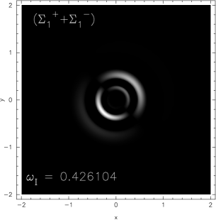
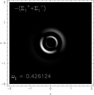
Figure 3: Gray-scale image of the positive component of real part of total surface density profile in $x-y$ plane at time $t=0$. White and black represent maximum and minimum/zero in the surface density for the model parameters same as that of fig. 2. Leading and trailing wave behaviour of the degenerate pairs of eigenvalues can be seen in the images. Plotting the negative of $\Sigma_{a}$ is motivated from the radial profile in the bottom panel of fig. 2.

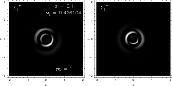
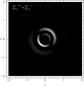
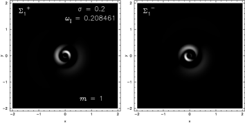
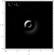
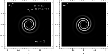
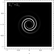
Figure 4: This plot displays the gray-scale image of density enhancement regions due to the perturbations for Kuzmin disc profile in the $x-y$ plane for time $t=0$. Plots are are labelled for their respective values of $\omega_{\text{\tiny{I}}},m\,\,\&\,\,\sigma$. Wavepackets are more radially compact for lower values of $\sigma\,\,\&\,\,m$.

6.2 Other values of $\eta$

In this subsection we present the results for values of $\eta$ other then $0\,\,\&\,\,1/2$. For these values, the discrete spectrum of eigenvalues we get are complex with non-zero real and imaginary parts, and we write $\omega=\omega_{\text{\tiny{R}}}+{\rm i}\omega_{\text{\tiny{I}}}$. Such modes are interesting as these correspond to growing/damping modes with the growth rate given by $\omega_{\text{\tiny{I}}}$ which also precess with the pattern speed given by $\omega_{\text{\tiny{R}}}$. We use $\eta=0.25\,\,\&\,\,0.4$ as test cases.

In fig. 5 and 6 we display the eigenvalues in complex argand plane. Fig. 5 is for Kuzmin disc and Fig. 6 is for JT annular disc. The panel labelled $(a)$ is for $\eta=0.25$ and the panel labelled $(c)$ is for $\eta=0.4$. First two rows are for $m=1$ and $\sigma=0.1\,\,\&\,\,0.2$ and bottom two rows are for $m=2$, for same values of velocity dispersion. The panel labelled $(b)$ and $(d)$ are the close-up view of regions near origin of the corresponding panels on the left. The horizontal lines are the real and continuous part of the spectrum. The continuum of eigenvalues corresponds to singular (van Kampen) modes. The eigenfunctions are concentrated at inner Lindblad resonances, which occurs at the radii for which $\omega=\pm m\dot{\varpi}$ (‘$\pm$’ signs are for prograde and retrograde discs respectively). Note that since for slow modes $\omega\ll\Omega$, the corotation and outer Lindblad resonances do not exist as is also pointed out by Gulati et al. (2012). Both the surface density profiles display the same behaviour for the continuous part of the eigenspectrum.

Coming to complex eigenvalues (or the discrete part of the spectrum), we get a wedge-like distribution, as the eigenvalues exist in complex conjugate pairs. For $\eta=0$ the eigenvalues are purely real, and as we increase the value of $\eta$ the spectrum goes from real to complex, until for $\eta=1/2$ the discrete spectrum is purely imaginary. This transition was first found by Touma (2002), and later by Gulati et al. (2012). A close-up view in panel $(b)\,\,\&\,\,(d)$ in fig. 5 we see that these two branches consists of more than one arm. These arms are due to the presence of degenerate pairs of eigenvalues corresponding to leading and trailing waves. Such pairs exists all throughout the branch. The separation in the degenerate pairs increases as we go to lower values of eigenvalues. Hence the arms separate out more prominently close to origin and go to zero with further decrease of eigenvalue. These arms were also noticed by Gulati et al. (2012) while studying the softened gravity disc. We do not see such prominent double-armed structure in the case of JT annular disc. This could probably be due to the fact that discrete spectrum itself is quite sparse. Secondly, in the case of JT annular disc, most of the disc mass is concentrated in an annular region, and as pointed by Jalali & Tremaine (2012) the degenerate pair of eigenvalues merge if the disc mass at resonances shrinks to zero. Touma (2002) have also studied softened gravity counter-rotating disc, applicable to planetary discs. The spectrum of eigenvalues the authors get is scattered and the plausible reason for this could be that the presence of degenerate pairs and the arms are not well defined due to sparse nature of the eigenvalues. For the variation with $m\,\,\&\,\,\sigma$, the largest growth rate is a decreasing function of $\sigma$ and $m$ both.

Eigenfunctions are in general complex. Fig. 7 is the gray-scale image of the positive component of the real part of the perturbed surface density, $\Sigma_{1}^{\pm}$ and $\Sigma_{1}^{+}+\Sigma_{1}^{-}$, for the Kuzmin disc as the unperturbed disc profile, $m=1$ and $\sigma=0.1$. Top row is for $\eta=0.25$ and $\omega=0.233082+{\rm i}0.351567$ whereas the second row is for $\eta=0.4$ and $\omega=0.094297+{\rm i}0.415009$. The density contrast is clearly lopsided, which is more prominent for higher values of $\eta$. In fig. 8 we display the snapshots of evolution of positive part of total surface density perturbation, where the panels are labelled for $\varphi_{P}=\omega_{\text{\tiny{R}}}t$ for the same parameters as that of top panel of fig. 7. Each one contains certain amount of lopsidedness. The pattern rotates at an angular speed given by $\omega_{\text{\tiny{R}}}$ and there is an overall increase in the magnitude as the system evolves (exponential increase in magnitude because of the presence of $\exp(\omega_{\text{\tiny{I}}}t)$).

Figure 5: Eigenvalue plot for $\eta=0.25$ (panel $(a)$ and $(b)$) and $\eta=0.4$ (panel $(c)$ and $(d)$) in complex Argand-plane for Kuzmin disc profile. panel $(a)$ and $(c)$ gives the whole spectrum whereas column $(b)$ and $(d)$ are the close-up view near origin of their corresponding plots on the left. panels are labelled for their respective values of $m\,\,\&\,\,\sigma$. Horizontal line gives the continuum of singular (van-Kampen) eigenmodes given by $\omega=-m\dot{\varpi}$. Discrete spectrum of eigenvalue forms a wedge like shape as the eigenvalues exists is complex conjugate pairs. Close view near the origin shows a double armed structure due to the presence of degenerate pairs of eigenvalues.

Figure 6: Eigenvalue plot in complex argand-plane for JT annular disc on the same lines as that of fig. 5. Major difference in the spectrum we see is in the discrete part of the spectrum. The eigenvalues are sparsely spaced and we do not see the prominent double armed structure as seen for Kuzmin disc.

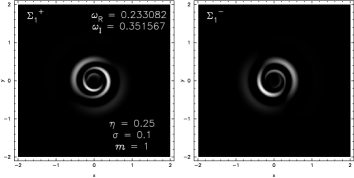
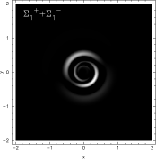
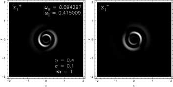
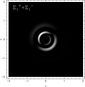
Figure 7: Gray-scale plot of the positive component of real part of $\Sigma_{a}^{\pm}(R)\exp({\rm i}(m\phi-\omega t))$ and $\Sigma_{a}^{+}(R)\exp({\rm i}(m\phi-\omega t))+\Sigma_{a}^{-}(R)\exp({\rm i}(m\phi-\omega t))$ at time $t=0$ for $\eta=0.25\,\,\&\,\,0.4$ in top and bottom panel respectively. First column is labelled for their respective values of $m,\,\,\sigma\,\,\&\,\,\omega$. Lopsidedness in the density profile is evident and is more prominent for higher value of $\eta$.

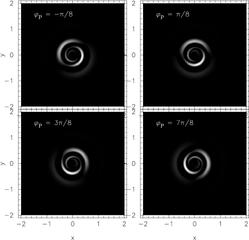
Figure 8: This plot displays the time evolution of total perturbed surface density for the same model parameters same as that in top panel of fig. 7. The plots are labelled for the value of $\varphi_{P}=\omega_{\text{\tiny{R}}}t$. Pattern rotates with angular speed given by $\omega_{\text{\tiny{R}}}$ along with an exponential increase in the intensity.

7 Summary and conclusions

We have formulated and analysed the modal behaviour of a system of two nearly Keplerian, counter-rotating axisymmetric stellar discs, rotating around a central mass. The formalism is a generalisation of the one studied in Paper I for a single disc, where we go one step beyond the usual WKB analysis by not assuming the relation between perturbed potential and surface density to be local. We first derived the integral eigenvalue equation for a tightly-wound linear modes of coplanar axisymmetric counter-rotating discs under the epicyclic approximation. Then, as an application of this equation, we restricted ourselves to near Keplerian systems—which support slow modes. We took the local limit of the integral equation to obtain the WKB dispersion relation to study the stability of the discs and concluded that (i) Counter-rotating discs are stable to axisymmetric perturbations if they satisfy the well known Toomre stability criterion. (ii) Non-axisymmetric perturbations are stable for a single disc, consistent with the conclusions of Sridhar & Saini (2010); Gulati et al. (2012); Jalali & Tremaine (2012) and Paper I. (iii) For non-zero mass in retrograde disc, discs are found to be largely unstable to non-axisymmetric perturbations.

Next we solved the integral eigenvalue equation for slow modes numerically. We used two different unperturbed surface density profiles, namely, Kuzmin disc, which is a centrally concentrated disc profile; and JT annular disc, which is a annular disc introduced by Jalali & Tremaine (2012). We assumed for both ‘$\pm$’ discs the same radial profile of velocity dispersion $\sigma_{R}=\sigma R\kappa(R)$ with $\sigma<1$. The same profile is also used in Paper I for a single disc, which was motivated by the work of Jalali & Tremaine (2012). We solved for various values of mass fraction, $\eta$ in the retrograde disc for $m=1\,\&\,2$. The spectrum for $\eta=0$ served as a test for our numerical methods, and the results obtained are in exact correspondence with those in Paper I. Following are the general properties of the spectrum and eigenfunctions obtained by us for all values of $\eta$.

• At $\eta=0$ the eigenvalues are all real and the modes are stable and oscillatory. As we increase the value of $\eta$, the eigenvalues become imaginary, with the value of highest growth rate increasing with increasing mass fraction in the retrograde disc till $\eta=1/2$. As we further increase $\eta$ the value of largest growth rate declines and the spectrum is again purely real (stable modes) for $\eta=1$.

• For no counter–rotation all the trends (discussed in the beginning of $\S~{}\ref{num_rslts}$) in the eigenspectrum and waveforms favour the observational detection of eigenmodes with lower values $m\,\,\&\,\,\sigma$.

• For equal counter–rotation, the highest growth rate for a given set of parameters decreases as a function of $\sigma\,\,\&\,\,m$, also favouring the excitation and hence detection of modes with lower values $\sigma\,\,\&\,\,m$.

• For other values of $\eta$, both real and imaginary parts of the eigenvalues are non-zero. The real part gives the pattern speed of the eigenfunction and imaginary part gives its growth rate.

• Eigenvalues exist in degenerate pairs, corresponding to leading and trailing waves, for all values of $\eta$. The presence of such degenerate pairs explains the presence of double-armed structure as seen the spectrum of eigenvalues for non-zero counter–rotation. Such double armed structure were also seen in Gulati et al. (2012).

• The separation between the degenerate pairs of eigenvalues increases with increasing $\sigma$ values and increasing number of nodes in the eigenfunction.

• The plot for surface density enhancement in the disc plane shows an overall lopsided intensity distribution for $m=1$, which is more prominent for higher values of $\eta$.

• The growth rate of pattern increases for higher values of $\eta$ and lower values of $m$, therefore allowing the $m=1$ instabilities to play a dominant role in the dynamics of such systems.

The calculated waveforms and their properties favour that these eccentric modes are the behind various non-axisymmetric features seen the discs like galactic nuclei, debris discs and accretion discs around stellar mass compact objects. Presence of retrograde mass in the disc gives rise to instabilities, thereby generating long lived, large scale features. A natural question to ask at this stage is how these counter–rotating streams of matter are formed in discs. In case of galaxies like M$31$, such retrograde orbits could be the result of in-fall of debris into the centres of such galaxies. Sambhus & Sridhar (2002) proposed that these stars could have been accreted to the centre of M31 in the form of a globular cluster that spiralled-in due to dynamical friction. For the in-falling mass in galactic nuclei, the sense of rotation will be uncorrelated with respect to the pre-existing material. Thus in the course of evolution of a galaxy, it is probable that counter-rotating systems are generically produced. Simulations by Nixon et al. (2012) show breaking of disc in the vicinity of rapidly rotating central massive object, and hence generically forming counter–rotating discs. Such counter–rotating streams of matter are also thought to be helpful in feeding massive black holes at centres of many galaxies.

Present work as well as the previous studies on slow modes for galactic discs are done assuming the disc to be composed of zero pressure fluid (gas) disc (Tremaine, 2001; Sambhus & Sridhar, 2002; Gulati et al., 2012) or collisionless disc composed of stars (Jalali & Tremaine (2012), Paper I). However in case of galaxies the gas/dust and the stellar discs exists together and are coupled to each other. In future we aim to formulate a theory of linear eigenmodes for discs composed of both stars and dust to study the nature of modes if both gas and stellar discs interact with each other only gravitationally. Recently Jalali (2013) have done a similar problem applicable only to protoplanetary discs using numerical simulations and found such systems to be unstable. We plan to extend our semi-analytical formulation to study the linear perturbation theory for such discs.

References

- Anderson et al. (1999) Anderson et. al. 1999, LAPACK Users’ Guide (3rd ed., Society for Industrial and Applied Mathematics)
- Araki (1987) Araki, S. 1987, Astron. J., 94, 99
- Binney & Tremaine (2008) Binney, J., & Tremaine, S. 2008, Galactic Dynamics (2ed., Princeton: Princeton University Press)
- Gulati et al. (2012) Gulati, M., Saini, T. D., & Sridhar, S. 2012, Mon. Not. Roy. Ast. Soc., 424, 348
- Gulati & Saini (2016) Gulati, M., & Deep Saini, T. 2016, arXiv:1601.04148
- Jalali & Tremaine (2012) Jalali, M. A., & Tremaine, S. 2012, Mon. Not. Roy. Ast. Soc., 421, 2368
- Jalali (2013) Jalali, M. A. 2013, Astroph. J. , 772, 75
- Lauer et al. (1993) Lauer, T. R., Faber, S. M., Groth, E. J., et al. 1993, Astron. J., 106, 1436
- Lauer et al. (1996) Lauer, T. R., Tremaine, S., Ajhar, E. A., et al. 1996, Astrophysical. J. Letters, 471, L79
- Lovelace et al. (1997) Lovelace, R. V. E., Jore, K. P., & Haynes, M. P. 1997, Astroph. J. , 475, 83
- Merritt & Stiavelli (1990) Merritt, D., & Stiavelli, M. 1990, Astroph. J. , 358, 399
- Murray & Dermott (1999) Murray, C. D., and Dermott, S. F. 1999, Solar System Dynamics (Cambridge: Cambridge University Press)
- Nixon et al. (2012) Nixon, C., King, A., Price, D., & Frank, J. 2012, Astrophysical. J. Letters, 757, L24
- Palmer & Papaloizou (1990) Palmer, P. L., & Papaloizou, J. 1990, Mon. Not. Roy. Ast. Soc., 243, 263
- Press et al. (1992) Press, W. H., Teukolsky, S. A., Vetterling, W. T., & Flannery, B. P. 1992, Numerical Recipes (2nd ed., Cambridge: University Press)
- Sellwood & Merritt (1994) Sellwood, J. A., & Merritt, D. 1994, Astroph. J. , 425, 530
- Sridhar & Saini (2010) Sridhar, S., & Saini, T.D. 2010, Mon. Not. Roy. Ast. Soc., 404, 527
- Sambhus & Sridhar (2002) Sambhus, N., & Sridhar, S. 2002, Astron. Astrophys., 388, 766
- Sawamura (1988) Sawamura, M. 1988, PASJ, 40, 279
- Toomre (1964) Toomre, A. 1964, Astroph. J. , 139, 1217
- Touma (2002) Touma, J. R. 2002, Mon. Not. Roy. Ast. Soc., 333, 583
- Tremaine (1995) Tremaine, S. 1995, Astron. J., 110, 628
- Tremaine (2001) Tremaine, S. 2001, Astron. J., 121, 1776
- Zang & Hohl (1978) Zang, T. A., & Hohl, F. 1978, Astroph. J. , 226, 521