A Rotating-Frame Perspective on High-Harmonic Generation of Circularly Polarized Light

Abstract

We employ a rotating frame of reference to elucidate high-harmonic generation of circularly polarized light by bicircular driving fields. In particular, we show how the experimentally observed circular components of the high-harmonic spectrum can be directly related to the corresponding quantities in the rotating frame. Supported by numerical simulations of the time-dependent Schrödinger equation, we deduce an optimal strategy for maximizing the cutoff in the high-harmonic plateau while keeping the two circular components of the emitted light spectrally distinct. Moreover, we show how the rotating-frame picture can be more generally employed for elliptical drivers. Finally, we point out how circular and elliptical driving fields show a near-duality to static electric and static magnetic fields in a rotating-frame description. This demonstrates how high-harmonic generation of circularly polarized light under static electromagnetic fields can be emulated in practice even at static field strengths beyond current experimental capabilities.

I Introduction

High-harmonic generation (HHG) of circularly polarized light was studied theoretically already in the 1990s Eichmann et al. (1995); Long et al. (1995); Becker et al. (1999); Milošević et al. (2000); Milošević and Becker (2000) but experimental demonstrations were not successful until very recently Fleischer et al. (2014); Kfir et al. (2015). The experimentally obtained high-harmonic spectra for such fields, including extensions towards elliptical drivers Fleischer et al. (2014), inspired theoretical efforts to provide simple explanations for the observed features, in particular with respect to conservation of photon angular momenta and corresponding selection rules Pisanty et al. (2014); Milošević (2015). Generating isolated circularly polarized high harmonics has been the subject of further theoretical Medišauskas et al. (2015) and experimental Hickstein et al. (2015) studies. Furthermore, it was shown recently that high-harmonic spectra with circular polarization can be made to reach even into the soft X-ray regime Fan et al. (2015).

At the base of most schemes for generation of high-harmonic circular light lies the use of a driving field that is a superposition of two copropagating but counter-rotating circular drivers with different frequencies. It has recently also been shown that counter-rotating drivers with the same frequency can be used when employing a non-collinear driving scheme Hickstein et al. (2015). In a somewhat different context, namely in the presence of additional static electromagnetic fields, HHG with such counter-rotating fields was also studied in the 2000s Milošević and Starace (1999); Bandrauk and Lu (2003). However, these studies neither considered the generated high-harmonic light in terms of its circularly polarized components nor did they report significant effects on the spectrum for readily available static magnetic and electric field strengths.

In this paper we show how a great deal of understanding of HHG with non-linearly polarized driving fields can be obtained by going to a rotating frame. Focusing on the paradigmatic case of counter-rotating bicircular drivers we illustrate how this allows to obtain a surprisingly simple characterization that even enables the formulation of optimal strategies for obtaining high-order harmonics with well-characterized circular polarization.

We begin by describing in Sec. II how a rotating frame of reference can be employed to obtain a single linearly polarized driving field from a bicircular driver in the lab frame. In Sec. III we show that there is a direct connection between the high-harmonic spectra in rotating frames and the lab frame when considering the circular components of the emitted light. This allows us to illustrate in Sec. IV that the most striking properties of the generation of circularly polarized high-harmonics can be very easily explained utilizing the linearizing rotating frame introduced in Sec. II. To emphasize this point even further we show in Sec. V how the rotating-frame description allows to formulate an optimal experimental strategy towards obtaining a high-harmonic plateau in the emission spectrum that is as far extended as possible while still separating the left and right circularly-polarized components energetically. We support these findings with numerical simulations of HHG on the single-atom level by solving the time-dependent Schrödinger equation for a two-dimensional model atom using the single-active-electron approximation. We finish our discussion by presenting two particular perspectives on the rotating-frame description: In Sec. VI we consider a more general setup involving elliptical driving fields and in Sec. VII we show how the study of HHG in rotating frames is strongly connected to questions concerning HHG in the presence of static electromagnetic fields. Finally, Sec. VIII concludes.

Atomic units are used throughout unless otherwise noted.

II The Linearizing Rotating Frame for Bicircular Drivers

We consider the Hamiltonian of an axially symmetric field-free Hamiltonian $H_{0}$ under the influence of the electric field of two counter-rotating circularly polarized laser pulses with envelope $F_{0}\left(t\right)$ and frequencies $\omega_{1},\omega_{2}$,

$$H\left(t\right) = H_{0}+F_{0}\left(t\right)\left[x\cos\left(\omega_{1}t\right)+y\sin\left(\omega_{1}t\right)\right.$$ (1)

$$\left.+x\cos\left(\omega_{2}t\right)-y\sin\left(\omega_{2}t\right)\right]\,.$$

The Hamiltonian (1) models an atom or a linear molecule aligned along the $z$-axis.

We will perform a unitary transformation on this Hamiltonian, first applied to HHG processes in Ref. Bandrauk and Lu (2003) and first mentioned in the explicit context of generation of circularly polarized high harmonics in Ref. Yuan and Bandrauk (2015), given by the following expression,

$$U\left(t\right)=e^{-i\alpha tL_{z}}\,,$$ (2)

with $L_{z}$ being the operator of angular momentum corresponding to rotation around the $z$-axis. Hence, Eq. (2) represents a rotation in the $x,y$-plane with angular frequency $-\alpha$. The rotating Hamiltonian reads

$$H^{\prime}\left(t\right) = U\left(t\right)HU^{\dagger}\left(t\right)-iU\left(t\right)\frac{\partial}{\partial t}U^{\dagger}\left(t\right)\,.$$

Clearly $U\left(t\right)H_{0}U^{\dagger}\left(t\right)=H_{0}$ due to the axial symmetry assumed for $H_{0}$. Furthermore

$$U\left(t\right)xU^{\dagger}\left(t\right) = x\cos\left(\alpha t\right)+y\sin\left(\alpha t\right)\,,$$

$$U\left(t\right)yU^{\dagger}\left(t\right) = y\cos\left(\alpha t\right)-x\sin\left(\alpha t\right)\,,$$

which allows us to transform the interaction term $H_{\text{int}}\left(t\right)=H\left(t\right)-H_{0}$ in Eq. (1) as follows,

$$U\left(t\right)H_{\text{int}}\left(t\right)U^{\dagger}\left(t\right) = F_{0}\left(t\right)\left[x\cos\left(\omega_{1}t\right)\cos\left(\alpha t\right)+y\cos\left(\omega_{1}t\right)\sin\left(\alpha t\right)+y\sin\left(\omega_{1}t\right)\cos\left(\alpha t\right)-x\sin\left(\omega_{1}t\right)\sin\left(\alpha t\right)\right.$$

$$\left.+x\cos\left(\omega_{2}t\right)\cos\left(\alpha t\right)+y\cos\left(\omega_{2}t\right)\sin\left(\alpha t\right)-y\sin\left(\omega_{2}t\right)\cos\left(\alpha t\right)+x\sin\left(\omega_{2}t\right)\sin\left(\alpha t\right)\right]\,.$$

Using the addition theorems of sine and cosine one arrives at the expression

$$U\left(t\right)H_{\text{int}}\left(t\right)U^{\dagger}\left(t\right)=F_{0}\left(t\right)\left(x\cos\left(\left[\omega_{1}+\alpha\right]t\right)+y\sin\left(\left[\omega_{1}+\alpha\right]t\right)+x\cos\left(\left[\omega_{2}-\alpha\right]t\right)-y\sin\left(\left[\omega_{2}-\alpha\right]t\right)\right)\,.$$ (3)

By choosing

$$\alpha=\frac{\omega_{2}-\omega_{1}}{2}$$ (4)

and defining the average frequency

$$\tilde{\omega}\equiv\frac{\omega_{1}+\omega_{2}}{2}=\omega_{1}+\alpha=\omega_{2}-\alpha\,.$$ (5)

we observe that the sine terms in Eq. (3) cancel and only a linearly polarized field with frequency $\tilde{\omega}$ remains. Hence we obtain for the total Hamiltonian in the rotating frame,

$$H^{\prime}\left(t\right)=H_{0}+\alpha L_{z}+2F_{0}\left(t\right)x\cos\left(\tilde{\omega}t\right)\,.$$ (6)

We will mostly focus on the case $\omega_{2}>\omega_{1}$ whence by Eq. (4) $\alpha>0$ follows.

We conclude that the dynamics of two counter-rotating circularly polarized driving fields can be interpreted as a single linearly polarized driver with double the field strength at the mean frequency. In the rotating frame an additional angular momentum term appears, which we will call coriolis term in accordance with Ref. Yuan and Bandrauk (2015), proportional to half the difference frequency. For two co-rotating circularly polarized drivers the result is almost identical and can be obtained by substituting $\omega_{2}\rightarrow-\omega_{2}$. The linearly polarized field in this case has a frequency equal to half the difference in frequency between the circular drivers while the coriolis term will now be equal to $\alpha^{\prime}L_{z}$ with $\alpha^{\prime}=\frac{\omega_{1}+\omega_{2}}{2}$ corresponding to the mean frequency.

III Translating Harmonic Spectra between Lab and Rotating Frames

How does one translate the harmonic signal of an atom or molecule from the rotating frame back to the lab frame? The high-harmonic signal in the lab frame has regularly been associated with the square of the Fourier transform of the dipole expectation value Corkum (1993); Bandrauk et al. (2008); Zhao and Zhao (2008), e.g., for the harmonic signal in $x$-direction one obtains

$$S_{x}^{\text{lab}}\left(\omega\right)=\left|\int D_{x}^{\text{lab}}\left(t\right)e^{-i\omega t}\ dt\right|^{2}=\left|\int\left\langle x\right\rangle_{\text{lab}}e^{-i\omega t}\ dt\right|^{2}\,,$$

where the expectation value $\left\langle\cdot\right\rangle_{\text{lab}}$ is taken with respect to the time-dependent wave function in the lab frame, $\ket{\psi\left(t\right)}$. Note that we already absorbed the minus sign from the dipole expectation value due to the electronic charge into the modulus. The wave function in the rotating frame is given by $U\left(t\right)\Ket{\psi\left(t\right)}$ with $U\left(t\right)$ given by Eq. (2). Using $U\left(t\right)U^{\dagger}\left(t\right)=U^{\dagger}\left(t\right)U\left(t\right)=\mathds{1}$ we obtain the expression

$$D_{x}^{\text{lab}}\left(t\right) = \left\langle x\right\rangle_{\text{lab}}=\left\langle\psi\left(t\right)|x|\psi\left(t\right)\right\rangle$$

$$= \left\langle\psi\left(t\right)|U^{\dagger}\left(t\right)U\left(t\right)xU^{\dagger}\left(t\right)U\left(t\right)|\psi\left(t\right)\right\rangle$$

$$= \left\langle x\right\rangle_{\text{rot}}\cos\left(\alpha t\right)+\left\langle y\right\rangle_{\text{rot}}\sin\left(\alpha t\right)\,,$$

where $\left\langle\cdot\right\rangle_{\text{rot}}$ denotes expectation values with respect to the time-dependent wave function in the rotating frame. The analogous expressions for the $y$-direction, $D_{y}^{\text{lab}}\left(t\right)$, as well as the right-circular component, $D_{+}^{\text{lab}}\left(t\right)$, and left-circular component, $D_{-}^{\text{lab}}\left(t\right)$, are given by

$$D_{y}^{\text{lab}}\left(t\right) = -\left\langle x\right\rangle_{\text{rot}}\sin\left(\alpha t\right)+\left\langle y\right\rangle_{\text{rot}}\cos\left(\alpha t\right)\,,$$

$$D_{+}^{\text{lab}}\left(t\right) = \frac{1}{\sqrt{2}}\left(D_{x}^{\text{lab}}\left(t\right)+iD_{y}^{\text{lab}}\left(t\right)\right)$$

$$= \frac{1}{\sqrt{2}}\left(\left\langle x\right\rangle_{\text{rot}}\cos\left(\alpha t\right)+\left\langle y\right\rangle_{\text{rot}}\sin\left(\alpha t\right)\right.$$

$$\left.+i\left\langle y\right\rangle_{\text{rot}}\cos\left(\alpha t\right)-i\left\langle x\right\rangle_{\text{rot}}\sin\left(\alpha t\right)\right)\,,$$

$$D_{-}^{\text{lab}}\left(t\right) = \frac{1}{\sqrt{2}}\left(D_{x}^{\text{lab}}\left(t\right)-iD_{y}^{\text{lab}}\left(t\right)\right)$$

$$= \frac{1}{\sqrt{2}}\left(\left\langle x\right\rangle_{\text{rot}}\cos\left(\alpha t\right)+\left\langle y\right\rangle_{\text{rot}}\sin\left(\alpha t\right)\right.$$

$$\left.-i\left\langle y\right\rangle_{\text{rot}}\cos\left(\alpha t\right)+i\left\langle x\right\rangle_{\text{rot}}\sin\left(\alpha t\right)\right)\,.$$

For the circular components the expressions can be significantly simplified by using cylindrical coordinates which leads to the expressions

$$D_{+}^{\text{lab}}\left(t\right) = \frac{1}{\sqrt{2}}\left\langle\rho e^{i\left(\varphi-\alpha t\right)}\right\rangle_{\text{rot}}\,,$$

$$D_{-}^{\text{lab}}\left(t\right) = \frac{1}{\sqrt{2}}\left\langle\rho e^{i\left(\varphi+\alpha t\right)}\right\rangle_{\text{rot}}\,,$$

where $x=\rho\cos\varphi$ and $y=\rho\sin\varphi$. This equation alludes to a direct connection between the harmonic spectra obtained in the rotating frame and the high-harmonic spectra in the lab frame. In fact, a short calculation shows that

$$S_{+}^{\text{lab}}\left(\omega\right) = \left|\int D_{+}^{\text{lab}}\left(t\right)e^{-i\omega t}\ dt\right|^{2}$$

$$= \left|\int\left\langle\frac{1}{\sqrt{2}}\rho e^{i\varphi}\right\rangle_{\text{rot}}e^{-i\left(\omega+\alpha t\right)}\ dt\right|^{2}$$

$$= S_{+}^{\text{rot}}\left(\omega+\alpha\right)\,,$$

$$S_{+}^{\text{lab}}\left(\omega-\alpha\right) = S_{+}^{\text{rot}}\left(\omega\right)$$ (7)

and analogously

$$S_{-}^{\text{lab}}\left(\omega\right) = S_{-}^{\text{rot}}\left(\omega-\alpha\right)\,,$$

$$S_{-}^{\text{lab}}\left(\omega+\alpha\right) = S_{-}^{\text{rot}}\left(\omega\right)\,.$$ (8)

We conclude that the right (left) circular signal in the lab frame is obtained via the right (left) circular signal in the rotating frame shifted in frequency by $\alpha$ to the left (to the right). We emphasize that this statement is general and no assumptions on $\alpha,\ \omega$ or the particular structure of $H_{0}$ (with the exception of its axial symmetry) have been made. This simple relationship between the circular spectral components in lab frame and rotating frame allows to directly apply any insights obtained about the high harmonic spectra in the rotating frame when discussing the experimentally observed spectra in the lab frame.

Finally, it should be pointed out that often the high-harmonic signal is associated with the Fourier transform of the dipole acceleration rather than that of the dipole moment Ivanov et al. (1996); Lein et al. (2002); Kamta and Bandrauk (2005). In Appendix A we show that computing the corresponding expectation values via Ehrenfest’s theorem with a slight modification allows to preserve the validity of Eqs. (7) and (8). The result from a formulation in terms of the dipole velocity can be derived by using the expressions from the dipole or the dipole acceleration with an appropriate scaling of the signal in terms of frequency Baggesen and Madsen (2011). Throughout the remainder of this work we compute high-harmonic spectra via the dipole acceleration using Ehrenfest’s theorem.

IV Understanding HHG Spectra from Analyses in Rotating Frames

In the linearizing rotating frame, the high-harmonic signal of right-circular, respectively left-circular, polarization is very similar to that of the system under a linearly polarized driver at the mean frequency, shifted with half the difference frequency up, respectively down, cf. Eqs. (4), (5), (7) and (8). The only difference to the well-studied HHG under a linearly polarized driver lies in the additional coriolis term $\alpha L_{z}$ in Eq. (6) that influences the system dynamics.

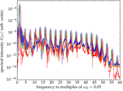
Figure 1: (color online) High-harmonic spectrum for two counter-rotating circular drivers with $\omega_{1}=\omega_{0}=0.05$, $\omega_{2}=2\omega_{1}=0.1$ and amplitude $F_{0}=0.05$ in the lab frame. The drivers are trapezoidally shaped with ramp time of 2 cycles, $T_{\text{ramp}}=\frac{4\pi}{\omega_{0}}$ and plateau time of 5 cycles, $T_{\text{plateau}}=\frac{10\pi}{\omega_{0}}$. The solid green (dark-shaded) curve is the right-circularly polarized signal in the lab frame, the solid orange curve (light-shaded) is the left-circularly polarized signal in the lab frame. The dashed blue (dark-shaded) curve is the signal in $x$-direction in the rotating frame (with $\alpha=0.025$) while the dashed red (light-shaded) curve is the signal in $y$-direction in the rotating frame. See Fig. 2 for a zoom-in.

To illustrate how a great deal of insight regarding HHG of circularly polarized light can be obtained by thinking in terms of rotating frames, we perform numerical simulations of the TDSE for a two-dimensional model atom in both lab frame and rotating frame. We will continue to call the prefactor of the coriolis term, corresponding to the negative rotation frequency of the rotating frame, $\alpha$. We look at the most prevalent example which has been studied by recent experiments - a counter-rotating circular driving scheme using a first and second harmonic Fleischer et al. (2014); Kfir et al. (2015), i.e., $\omega_{1}=\omega_{0}$ and $\omega_{2}=2\omega_{0}$, cf. Eq. (1). Transforming to a rotating frame with $\alpha=0.5\omega_{0}$ [Eq. (4)] we obtain $\tilde{\omega}=1.5\omega_{0}$ [Eq. (5)]. Because our arguments do not depend on a particular atomic or molecular species we were able to use identical simulation parameters as in a recent theoretical study that involved numerical simulations with a TDSE in two dimensions for such a set of bicircular counter-rotating drivers, cf. Table I in Ref. Medišauskas et al. (2015). The only numerical difference in our simulation consists in a slightly different complex absorber and us employing a Chebyshev propagator Tal-Ezer and Kosloff (1984) with a Fourier method for the kinetic energy. Matching the parameters to the $s$ ground state calculation performed in Medišauskas et al. (2015) we employ the screened potential $V\left(x,y\right)=V\left(\rho\right)=\frac{1}{\sqrt{\rho^{2}+0.1195}}$ leading to an ionization potential of $I_{p}=0.7935$. This allowed us to confirm the adequacy of our numerics by using our code to reproduce Fig. 1(a) of Ref. Medišauskas et al. (2015) in very good agreement .

With this set of parameters we now turn to analyze a high-harmonic spectrum in a rotating frame with $\alpha=0.025$. The driving field in this frame is given by a trapezoidally shaped laser pulse with frequency $\tilde{\omega}=0.075$ corresponding to a wavelength of $\sim 911\ \text{nm}$. The laser pulse is linearly polarized along the $x$-direction and its maximal electric field strength is given by $2F_{0}=0.1$. The linear ramp-up and ramp-down time is given by $T_{\text{ramp}}=251.33$ and the plateau width is given by $T_{\text{ramp}}=628.32$. In the lab frame this corresponds to a right-circularly polarized driver superimposed with a counter-rotating left-circularly polarized driver with frequencies $\tilde{\omega}-\alpha=0.05=\omega_{1}=\omega_{0}$, respectively $\tilde{\omega}+\alpha=0.1=\omega_{2}=2\omega_{0}$, both with peak amplitude $F_{0}=0.05$.

In the rotating frame we can formulate the well-known selection rules of HHG driven by a linearly polarized pulse, i.e., we obtain a signal only at odd multiples of $\tilde{\omega}$. Note that these selection rules are not altered by the coriolis term since it neither breaks the inversion symmetry nor the conservation of $L^{2}$ and $L_{z}$. In the lab frame we obtain accordingly by Eqs. (7) and (8) a signal from a right, respectively left, circularly polarized field at frequencies $\left[\left(2n+1\right)\tilde{\omega}-\alpha\right]$ and $\left[\left(2n+1\right)\tilde{\omega}+\alpha\right]$ ($n\in\mathbb{N}_{0}$) corresponding to $\left(3n+1\right)\omega_{0}$ and $\left(3n-1\right)\omega_{0}$ which is consistent with the selection rules obtained in experiments Fleischer et al. (2014); Hickstein et al. (2015) and previous theoretical studies Alon et al. (1998); Ceccherini et al. (2001); Nilsen et al. (2002). This behavior is confirmed by our numerical results, cf. Figs. 1 and 2. If we ignore the coriolis term in the rotating frame we have emission purely in the $x$-direction and as such the height of the two opposite circularly polarized peaks originating from a given (linearly polarized) harmonic in the rotating frame would be equal. However, the coriolis term does have a non-vanishing effect on the direction of the emission in the rotating frame and there is a visible contribution in the $y$-direction which can be directly associated with the difference in peak heights. For most peaks the contribution from the $y$-direction in the rotating frame for this particular set of parameters is about one order of magnitude smaller than the contribution from the $x$-direction. This explains the mostly close peak heights of neighboring left- and right-circular harmonics in the lab frame, cf. Figs. 1 and 2.

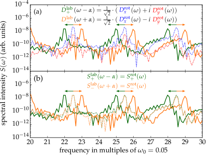
Figure 2: (color online) (a) Zoomed-in high-harmonic spectra from Fig. 1 illustrating the spectral shifts between rotating frame and lab frame. (b) Same as (a) but with rotating frame spectra also shown in terms of right- and left-circular components. The equations above the curves show the relations discussed in Sec. III between (a) dipole amplitudes and (b) spectral intensities in lab and rotating frame.

We can even go a step further and understand the temporal generation process of the circularly polarized light from the perspective of the rotating frame. The highest ionization probability, which according to the three-step model Corkum (1993); Schafer et al. (1993); Lewenstein et al. (1994) forms the starting point of HHG, occurs around the peaks of the electric field. In the rotating frame this means we have bursts of linearly polarized light at minima and maxima of the electric field with frequency $\tilde{\omega}=1.5\omega_{0}$. In terms of the period of the first harmonic driver $T=\frac{2\pi}{\omega_{0}}$ we consequently obtain bursts of linearly polarized high-harmonic radiation at $t=0,\frac{2\pi}{3\omega_{0}},\frac{4\pi}{3\omega_{0}},\frac{2\pi}{\omega_{0}},\ldots=0,\frac{T}{3},\frac{2T}{3},T,\ldots$. As discussed above, at least for moderately small coriolis terms, we can approximate all emission in the rotating frame to take place along the $x$-direction. At $t=0$ both frames are identical hence $t=0$ corresponds to a polar angle of $\varphi=0$. If we associate the times of high harmonic emission with corresponding angles with the lab-frame $x$-axis we arrive at pairs $\left(t,\varphi\right)=\left(0,0\right)$, $\left(\frac{T}{3},\frac{5\pi}{3}\right)$, $\left(\frac{2T}{3},\frac{4\pi}{3}\right)$, $\left(T,\pi\right)$, $\ldots$. However, we note that the emission of high-harmonic bursts can occur at both maxima and minima of the driving field. Since the driving field is linearly polarized in $x$-direction in the rotating frame we can relate these maxima and minima by considering a mirroring at the rotating-frame $y$-axis. Such a mirroring leads to a shift of the emission angle in the lab frame by $\pi$. Consequently, taking into account both emission around a maximum and a minimum of the electric field, we obtain the following time-angle pairs: $\left(t,\varphi\right)=\left(0,0\right)$, $\left(\frac{T}{3},\frac{2\pi}{3}\right)$, $\left(\frac{2T}{3},\frac{4\pi}{3}\right)$, $\left(T,0\right),\left(\frac{4T}{3},\frac{2\pi}{3}\right)$, $\left(\frac{5T}{3},\frac{4\pi}{3}\right)$, $\left(2T,0\right)$, $\ldots$. This corresponds precisely to the emission pattern predicted by previous works Milošević et al. (2000); Milošević and Becker (2000) in which in each cycle of the fundamental driver three linearly polarized emission bursts are predicted, each rotated by an angle of $120^{\circ}$ with respect to each other.

V Optimizing the HHG Spectrum for Bicircular Driving

For a fixed frequency $\tilde{\omega}$ [Eq. (5)] and field strength $F_{0}$ of the linearly polarized field in the linearizing rotating frame, any bicircular driving scheme in the lab frame is characterized by a single parameter: $\alpha$. For $\alpha=0$, we expect due to the linear driving in the rotating frame a high-harmonic cut-off according to the semiclassical limit at $I_{p}+3.17U_{p}$, with $I_{p}$ the ionization potential and $U_{p}=\frac{F_{0}^{2}}{4\tilde{\omega}^{2}}$ the ponderomotive potential. Even including the effect of the coriolis term, it seems natural to expect that a decrease in $\tilde{\omega}$, respectively an increase in $F_{0}$, will still lead to an extension of the high-harmonic plateau by increasing the ponderomotive potential. This leaves the question regarding the role of $\alpha$ on the spectral cut-off.

We show in Fig. 3 the high-harmonic spectrum in the lab frame for $\tilde{\omega}=0.05$ and $F_{0}=0.1$ for otherwise identical parameters as in Sec. IV. Note that $\tilde{\omega}$ refers to the mean frequency of the counter-rotating drivers. For $\alpha=0$, cf. Fig. 3(a), lab frame and rotating frame are identical, and the driving field is linearly polarized in both. The high-harmonic signal in the $y$-direction is consequently zero. Hence, the right-circular and left-circular signals are identical and one clearly observes the expected behavior of spectral peaks at odd multiples of the laser frequency in the high-harmonic plateau. The plateau cut-off at around $E_{\text{cutoff}}\simeq 80\tilde{\omega}=4.00$ matches perfectly with the semi-classical prediction at $I_{p}+3.17U_{p}=3.97$.

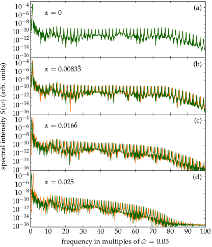
Figure 3: (color online) High-harmonic spectrum in the lab frame for fixed $\tilde{\omega}$ and $F_{0}$ and different values of $\alpha$. The green (dark-shaded) curve represents the right-circular spectrum, while the orange (light-shaded) curve represents the left-circular spectrum (in panel (a) both are on top since the signal in $y$-direction vanishes for $\alpha=0$).

Increasing the value of $\alpha$ gradually depresses the high-harmonic plateau, cf. Fig. 3(b)-(d). This effect can be rationalized by a simple semiclassical argument. For higher harmonics the excursion of the electron needs to be further and further away from the nucleus, corresponding to a higher energy gain in the electric field in the framework of the three-step model. However, the larger the distance from the nucleus the stronger the effect of the $L_{z}$-term will be which leads to acceleration of the electron in the $y$-direction. This deflection will reduce the $x$-elongation in favor of the $y$-elongation. As a consequence the energy acquired by the electron in the electric field is reduced as it is proportional to only the $x$-component of its elongation since the laser pulse is linearly polarized in $x$-direction in the rotating frame. Incidentally, this also allows for a simple explanation on why counter-rotating drivers are significantly more suitable than co-rotating drivers if one aims to obtain circularly polarized high-harmonics. In a co-rotating scheme $\alpha$ is not given by half of the difference of the frequencies of the two drivers in the lab frame but by the average of their frequencies. This immediately implies a much larger value of $\alpha$ leading to a much stronger depression of the high-harmonic plateau compared to an equivalent counter-rotating scheme.

Looking at the high-harmonic spectra from Fig. 3, shifted according to Eqs. (7) and (8) to obtain the circular components of the harmonic signal in the lab frame, one can observe an interesting dichotomy. On the one hand our results clearly show that using two drivers that are as close in frequency as possible leads to the least reduction in the high-harmonic plateau, on the other hand one requires a sufficiently large $\alpha$ to obtain spectrally separated signals for the two circular polarization directions in the lab frame. The width of the harmonic peaks is primarily determined by the temporal width of the drivers. Hence, the optimal strategy to obtain spectral selectivity for the two polarization directions while having a harmonic plateau that is as far extended as possible consists in choosing $\alpha$ just above the spectral width of the harmonic peaks. Specifically, for the typically chosen ‘fundamental plus second harmonic’ driving scheme, shown in Fig. 3(c), we observe that our particular chosen set of parameters would still allow closer frequencies for the bicircular drivers while maintaining a sufficient spectral separation of the right-circular and left-circular harmonic peaks, cf. Fig. 3(b).

From an experimental point of view this means that for driving pulses with several optical cycles the best results will be obtained by choosing driving fields originating from a laser with frequency $\omega_{0}$ where the left-circularly polarized driver is tuned lower by a small amount while the right-circularly polarized driver is tuned higher by the same amount (or vice versa). Conversely, if the driving fields consist of only very few cycles then the spectral width of the peaks will increase and it is likely that choosing low-order harmonics of a fundamental frequencies is a more suitable approach. In particular, employing a left-circularly polarized driver at some fundamental $\omega_{0}$ and a right-circularly polarized driver at the third harmonic $3\omega_{0}$ leads to $\tilde{\omega}=2\omega_{0}$ and a maximal spectral separation of the peaks in the high-harmonic spectrum given by $\tilde{\omega}$. However, this comes with a cost, namely a coriolis term in the rotating frame with strength $\alpha=\omega_{0}$. This represents already a moderately strong depression of the high harmonic plateau, cf. Fig. 3(d).

VI Perspectives for Rotating Frame Analyses I: Elliptical drivers

We can generalize Eq. (1) to the case of one of the two drivers having elliptical polarization instead of circular polarization, a situation that has been recently explored experimentally Fleischer et al. (2014) and also discussed from a theoretical point of view Pisanty et al. (2014); Milošević (2015). The Hamiltonian in this case can be written as

$$H\left(t\right) = H_{0}+F_{0}\left(t\right)\left(A\left(\epsilon\right)x\cos\left(\omega_{1}t\right)+B\left(\epsilon\right)y\sin\left(\omega_{1}t\right)\right.$$ (9)

$$\left.+x\cos\left(\omega_{2}t\right)-y\sin\left(\omega_{2}t\right)\right)\,,$$

where $A\left(\epsilon\right)=\frac{\sqrt{2}}{\sqrt{1+\epsilon^{2}}}$ and $B\left(\epsilon\right)=\frac{\sqrt{2}\epsilon}{\sqrt{1+\epsilon^{2}}}$, with $\epsilon$ being the ellipticity of the field with frequency $\omega_{1}$. The case $\epsilon=1$ leads back to the case of bicircular driving with equal strengths whereas $\epsilon=0$ corresponds to the superposition of a linearly polarized field with a left-circularly polarized one. Following the steps from Sec. II, by going into a rotating frame with frequency $-\alpha$ we arrive at the intermediate expression

$$H^{\prime} = H_{0}+\alpha L_{z}$$

$$+F_{0}\left(t\right)\left\{\frac{1}{2}\left(A+B\right)\left(x\cos\left(\left[\alpha+\omega_{1}\right]t\right)+y\sin\left(\left[\alpha+\omega_{1}\right]t\right)\right)\right.$$

$$+\frac{1}{2}\left(A-B\right)\left(x\cos\left(\left[\omega_{1}-\alpha\right]t\right)-y\sin\left(\left[\omega_{1}-\alpha\right]t\right)\right)$$

$$\left.\vphantom{\frac{1}{2}}+x\cos\left(\left[\omega_{2}-\alpha\right]t\right)-y\sin\left(\left[\omega_{2}-\alpha\right]t\right)\right\}\,.$$

For brevity we suppress the $\epsilon$ dependence of $A$ and $B$. An ‘on-frequency’ co-rotating frame is obtained by choosing $\omega_{1}=\alpha$ leading to the rotating-frame Hamiltonian

$$H^{\prime} = H_{0}+\omega_{1}L_{z}+\frac{1}{2}\left(A-B\right)F_{0}\left(t\right)x$$ (10)

$$+F_{0}\left(t\right)\left\{\frac{1}{2}\left(A+B\right)\left(x\cos\left(2\omega_{1}t\right)+y\sin\left(2\omega_{1}t\right)\right)\right.$$

$$\left.\vphantom{\frac{1}{2}}+x\cos\left(\left[\omega_{2}-\omega_{1}\right]t\right)-y\sin\left(\left[\omega_{2}-\omega_{1}\right]t\right)\right\}\,,$$

which can be interpreted as the system being subject to two counter-rotating circular drivers with different amplitude in the presence of a coriolis term and a static electric field. While this field is not truly static since it is modified by the pulse envelope the timescale of this modulation is slow enough such that the electric field can be regarded as static for the purposes of HHG except for extremely short drivers. For $A=B$ ($\epsilon=1$) we reobtain the case from Sec. II which manifests through a vanishing static electric field term in the rotating frame.

The shift property for the HHG spectra between rotating frame and lab frame of circular emission components, cf. Sec. III, allows once again to use symmetry arguments in the rotating frame to obtain information about the actual HHG spectrum in the lab frame. For $A=B$ it can easily be seen from Eq. (10) that in the time-independent Hamiltonian $L_{z}$ is conserved which means that emission can only take place with $\left(n+1\right)$ photons from the right-circular driver and $n$ from the left-circular driver, respectively $\left(n-1\right)$ photons from the right-circular driver and $n$ photons from the left circular driver Pisanty et al. (2014); Kfir et al. (2015); Milošević (2015). This leads in the first case to right-circularly polarized emission at frequencies $n\left(\omega_{1}+\omega_{2}\right)+\left(\omega_{2}-\omega_{1}\right)$, corresponding to a right-circularly polarized field in the lab frame at $n\left(\omega_{1}+\omega_{2}\right)+\omega_{2}-2\omega_{1}$, respectively left-circularly polarized emission at frequencies $n\left(\omega_{1}+\omega_{2}\right)-\left(\omega_{2}-\omega_{1}\right)$, corresponding to a left-circularly polarized field in the lab frame at $n\left(\omega_{1}+\omega_{2}\right)-\left(\omega_{2}-2\omega_{1}\right)$.

Once $A$ starts to deviate from $B$ both a breaking of inversion symmetry and a breaking of conservation of the angular momentum occur in the ‘static’ Hamiltonian. This opens up arbitrary combinations of the driving fields at frequencies $\left(2n-m\right)\omega_{1}+m\omega_{2}$ where $n>m$ corresponds to right-circular signals, which appear in the lab frame at $\left(2n-m-1\right)\omega_{1}+m\omega_{2}$, and $n<m$ corresponds to left-circular signals, which appear in the lab frame at $\left(2n-m+1\right)\omega_{1}+m\omega_{2}$. The case $n=m$ corresponds to linear emission channels at frequencies $n\left(\omega_{1}+\omega_{2}\right)$ with equal contributions from the counter-rotating circular drivers in the rotating frame. This channel will split in the lab frame into two signals: a right-circularly polarized signal at $n\left(\omega_{1}+\omega_{2}\right)-\omega_{1}$ and a left-circularly polarized signal at $n\left(\omega_{1}+\omega_{2}\right)+\omega_{1}$. Note that the larger the discrepancy between $A$ and $B$ the more dominant contributions with greater difference between $n$ and $m$ will become. This is because the intensity ratio between the $n$-right-circular driver and $m$-left-circular driver in the rotating frame goes as $\frac{I_{n}}{I_{m}}=\frac{\left(A+B\right)^{2}}{4}=\frac{1}{2}+\frac{\epsilon}{1+\epsilon^{2}}$ which is a monotonously increasing function for $\epsilon\in\left[-1,1\right]$. Additionally, the more $A$ and $B$ differ the stronger the static field term becomes which leads to larger and larger symmetry breaking, washing out the HHG among more and more channels.

In light of the importance of the difference between $n$ and $m$ it is useful to define $\bar{n}\equiv n-m$. Then, we can state the following: One observes left circularly polarized signals in the lab frame at frequencies $\left(2\bar{n}+m-1\right)\omega_{1}+m\omega_{2}$ for $\bar{n}\geq 0$ and right-circularly polarized signals in the lab frame at frequencies $\left(2\bar{n}+m+1\right)\omega_{1}+m\omega_{2}$ for $\bar{n}\leq 0$. The principal order of the signal is given by $m$ whereas $\left|\bar{n}\right|$ reflects the required symmetry breaking where the breaking strength is proportional to the deviation of $\left|\bar{n}\right|$ from $1$, with only $\left|\bar{n}\right|=1$ corresponding to symmetry conservation. These findings match perfectly with those in Ref. Milošević (2015).

VII Perspectives for Rotating Frame Analyses II: Static Electric and Magnetic Fields

In addition to the appearance of a static electric field term by entering a rotating frame as in Sec. VI there is also an interesting connection to static magnetic fields for both the rotating-frame descriptions obtained in Secs. II and VI. This becomes clear when considering an axially symmetric system under the influence of a static magnetic field along the $z$-direction, $\vec{B}=B_{0}\vec{e}_{z}$. The full Hamiltonian in Coulomb gauge reads in this case

$$H_{\text{mag}} = H_{0}+\frac{B_{0}}{2}L_{z}+\frac{B_{0}^{2}}{8}\left(x^{2}+y^{2}\right)\,.$$ (11)

The angular momentum term appearing in this context has an identical form to the coriolis term obtained for rotating-frame Hamiltonians, but there is an additional contribution that leads to harmonic trapping along the $z$-axis proportional in strength to the square of the magnetic field. It should be pointed out, however, that this term does preserve the axial symmetry of $H_{0}$ and thus will not alter the harmonic spectrum in terms of symmetry-forbidden harmonics. Still, similarly to the coriolis term, the signal strength of the emitted higher harmonics will be reduced by this term since long excursions from the nucleus are suppressed. Furthermore a ‘true’ static magnetic field in the lab frame readily allows to tune the harmonic term and the coriolis term independently since the strength of the harmonic term is invariant under a transformation to the rotating frame while the total coriolis term will have strength $B_{0}+\alpha$ where $\alpha$ is the rotation frequency of the rotating frame. This allows to independently study the effects of both contributions in a practical setup.

We want to briefly address the fact that the initial state for HHG can be different in the magnetic field case compared to the case of merely considering a rotating frame. This can for example occur when the presence of the magnetic field breaks the symmetry in a degenerate ground state manifold. In this case the ground state of $H_{\text{mag}}$ will not follow the symmetries of $H_{0}$. This may significantly alter the HHG spectrum as high-harmonic spectra show a clear dependence on the initial state of the system, see, e.g., Ref. Medišauskas et al. (2015) for an analysis with respect to bicircular drivers. For high magnetic fields it is also conceivable that an excited state with, e.g., $p$ character becomes energetically lowered below the energy of the ground state with $s$ character (which is unaffected by a Zeeman splitting). However, if the magnetic field is established sufficiently slowly the ground state will likely remain invariant due to adiabatic following. For the case of static electric fields very similar arguments hold.

Previous theoretical studies in terms of static electric and magnetic fields concluded that an appreciable impact on the HHG spectra can only be observed for field strengths at the very edge of experimental feasibility Milošević and Starace (1999); Bandrauk and Lu (2003). In a rotating-frame picture these field strengths are achieved rather naturally since they originate from AC field strengths (for electric fields), respectively from the frequency of the rotating-frame description (for magnetic fields). For example, using an $800$ nm right-circularly polarized driver and its second harmonic at $400$ nm as a left-circularly polarized driver, the linearizing rotating frame as discussed in Sec. II leads to a coriolis term which would correspond by Eq. (11) to a static magnetic field of almost $12000$ T.

Circular high-harmonic emission in the lab frame and the rotating frame are directly related to each other by only a shift in frequency, cf. Sec. III. This allows on the one hand to directly apply knowledge about static-field effects to understanding high harmonic spectra of circular light while on the other hand enabling the possibility to engineer Hamiltonians in the rotating frame that realize the effects of such static fields even at field strengths beyond current technical feasibility.

VIII Conclusions

HHG of circularly polarized light with bicircular drivers can be understood in many ways, ranging from a purely photonic picture to a strictly classical four-wave mixing interpretation Pisanty et al. (2014). A particularly simple way to approach this process is by moving to a rotating frame of reference where the bicircular driving reduces to a linearly polarized field and a coriolis term Bandrauk and Lu (2003); Yuan and Bandrauk (2015). We showed in this paper that the circularly polarized components of the high-harmonic signal in the lab frame follow directly from their counterparts in the rotating frame under a simple shift in frequency. This allows to directly deduce properties of those spectra and even the generation process itself from the well-studied HHG with linearly polarized driving fields. The influence of the coriolis term for axially symmetric systems on the high-harmonic plateau consists in a reduction of the cutoff frequency proportional to the strength of this term. Otherwise it does not alter the peak structure in the spectrum due to the preservation of the axial symmetry. As a consequence it is possible to determine the optimal bicircular drivers when the goal is to preserve a high-harmonic plateau that is extended as far as possible - the drivers need to be counter-rotating and their frequencies should be chosen as similarly as possible. Only the need for a spectral separation of the two circularly polarized components requires to choose a nonzero difference in frequency to compensate for the finite width of the peaks in frequency domain due to the finite width of the driving fields in time. Conversely, if such a spectral separation is not necessary because the right and left-circularly polarized signal can be otherwise filtered out, choosing identical frequencies is clearly the best approach. This is an observation that very recently has been made in an experimental study where circularly polarized high harmonics have been generated in a non-collinear scheme allowing for a spatial separation of the two circularization directions Hickstein et al. (2015).

Beyond the case of bicircular drivers, a rotating-frame picture also offers a valuable perspective on elliptical drivers. The occurrence of additional peaks in the high-harmonic spectrum when moving away from the bicircular case originates in a properly chosen rotating frame from the presence of an additional static electric field. This static electric field breaks the symmetries present for bicircular drivers and opens up additional channels for HHG in the rotating frame that can then be directly observed in the lab frame taking into account the corresponding shift in frequency. Furthermore, the rotating-frame description of these schemes shows a near-duality to HHG under static electric and magnetic fields. While the effects of such fields have been examined in the past, the regime in which a visible impact on the spectra could be experimentally observed is mostly inaccessible due to the infeasibility of generating the corresponding strong fields. However, the rotating-frame picture clearly illustrates that the effect of such strong fields appear naturally in a suitably chosen frame of reference and the resulting modifications of the high-harmonic spectra of these ‘virtual’ fields have clearly observable consequences in experiments that can readily be performed today.

The rotating-frame picture proves to be a powerful tool in understanding HHG of circularly polarized light. Depending on the particular choice of driving fields it enables a close correspondence to linearly polarized drivers and even HHG in the presence of static electric and magnetic fields. It can thus serve as a pivotal link between seemingly disjoint setups for HHG and allows for a remarkably simple explanation of many properties of the experimentally observed spectra.

Appendix A HHG Spectra via Dipole Acceleration in Rotating Frames

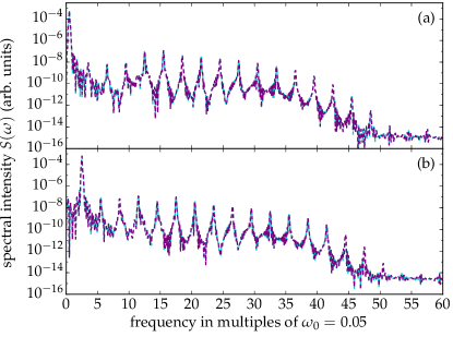
Figure 4: (color online) (a) High-harmonic spectrum for the right-circularly polarized field component and (b) the left-circularly polarized field component for two counter-rotating fields with frequency $\omega_{1}=\omega_{0}=0.05$, respectively $\omega_{2}=2\omega_{0}=0.1$, with equal field amplitude of $F_{0}=0.05$. The driving laser pulse is trapezoidally shaped with the same parameters as in Fig. 1. The turquoise (light-shaded) curves are the results in the lab frame, the purple (dark-shaded) curves are the results in a rotating frame with rotation frequency $\alpha=0.025$ shifted to the left by $\alpha$ for right-circular polarization, respectively to the right by $\alpha$ for left-circular polarization.

The expectation value of the dipole acceleration can be computed via Ehrenfest’s theorem,

$$\left\langle\vec{a}\right\rangle=\frac{d^{2}}{dt^{2}}\left\langle\vec{x}\right\rangle=\frac{d}{dt}\left\langle\vec{p}\right\rangle=-\left\langle\vec{\nabla}V\right\rangle\,.$$

We can then perform the following calculation ,

$$\left\langle\vec{a}\right\rangle_{\text{lab}} = \frac{d}{dt}\left\langle\vec{p}\right\rangle_{\text{lab}}$$

$$= \frac{d}{dt}\left\langle U^{\dagger}\left(t\right)U\left(t\right)\vec{p}U^{\dagger}\left(t\right)U\left(t\right)\right\rangle_{\text{lab}}$$

$$= \frac{d}{dt}\Braket{\psi_{\text{rot}}\left(t\right)}{e^{-i\alpha tL_{z}}\vec{p}e^{i\alpha tL_{z}}}{\psi_{\text{rot}}\left(t\right)}$$

$$= i\Braket{\psi_{\text{rot}}\left(t\right)}{\left[H_{\text{rot}},e^{-i\alpha tL_{z}}\vec{p}e^{i\alpha tL_{z}}\right]}{\psi_{\text{rot}}\left(t\right)}$$

$$+\Braket{\psi_{\text{rot}}\left(t\right)}{e^{-i\alpha tL_{z}}\left[-i\alpha L_{z},\vec{p}\right]e^{i\alpha tL_{z}}}{\psi_{\text{rot}}\left(t\right)}$$

$$= i\Braket{\psi_{\text{rot}}\left(t\right)}{\left[H_{0}+\alpha L_{z},e^{-i\alpha tL_{z}}\vec{p}e^{i\alpha tL_{z}}\right]}{\psi_{\text{rot}}\left(t\right)}$$

$$-i\alpha\Braket{\psi_{\text{rot}}\left(t\right)}{e^{-i\alpha tL_{z}}\left[L_{z},\vec{p}\right]e^{i\alpha tL_{z}}}{\psi_{\text{rot}}\left(t\right)}$$

$$= i\Braket{\psi_{\text{rot}}\left(t\right)}{\left[H_{0},e^{-i\alpha tL_{z}}\vec{p}e^{i\alpha tL_{z}}\right]}{\psi_{\text{rot}}\left(t\right)}\,.$$

For the right-circular component of the acceleration this means that

$$\left\langle a_{+}\right\rangle_{\text{lab}}$$

$$=i\frac{1}{\sqrt{2}}\Braket{\psi_{\text{rot}}\left(t\right)}{\left[H_{0},e^{-i\alpha tL_{z}}\left(p_{x}+ip_{y}\right)e^{i\alpha tL_{z}}\right]}{\psi_{\text{rot}}\left(t\right)}$$

$$=i\frac{e^{-i\alpha t}}{\sqrt{2}}\Braket{\psi_{\text{rot}}\left(t\right)}{\left[H_{0},p_{x}+ip_{y}\right]}{\psi_{\text{rot}}\left(t\right)}$$

$$=-\frac{1}{\sqrt{2}}e^{-i\alpha t}\left[\left\langle\nabla_{x}V\right\rangle_{\text{rot}}+i\left\langle\nabla_{y}V\right\rangle_{\text{rot}}\right]$$

$$=-e^{-i\alpha t}\left\langle\nabla_{+}V\right\rangle_{\text{rot}}\,,$$

where $V$ is the potential term in the Hamiltonian $H_{0}$ and $\nabla_{\pm}\equiv\frac{1}{\sqrt{2}}\left(\nabla_{x}\pm i\nabla_{y}\right)$.

As a consequence one obtains the high-harmonic signal for the right-circular component via

$$S_{+}^{\text{lab}}\left(\omega\right) = \left|\int\left\langle a_{+}\right\rangle_{\text{lab}}e^{-i\omega t}\ dt\right|^{2}$$

$$= \left|\int\left\langle\nabla_{+}V\right\rangle_{\text{rot}}e^{-i\left(\omega+\alpha\right)t}\ dt\right|$$

$$= S_{+}^{\text{rot}}\left(\omega+\alpha\right)\,,$$

which represents a shift of the high-harmonic signal in right-circular direction obtained in the rotating frame in direct analogy to the case for the expectation value of the dipole, cf. Eq. (7). The derivation for the left-circular direction can be performed analogously leading to the respective result as in Eq. (8). An important point to emphasize is that when using Ehrenfest’s theorem in the rotating frame one needs to compute the derivative of the potential term corresponding to the non-rotating Hamiltonian, i.e., the coriolis term does not enter.

A comparison of the high-harmonic spectrum obtained via Ehrenfest’s theorem in the rotating frame versus the lab frame is shown in Fig. 4. Evidently, both results match extraordinarily well. The remaining discrepancies stem from the fact that the spectral grid points of the shifted spectrum from the rotating frame and those of the unshifted spectrum from the lab frame do not quite match since the time grid we employed leads to a distance between two grid points in frequency domain that is no integer multiple of $\alpha$.

References

- Eichmann et al. (1995) H. Eichmann, A. Egbert, S. Nolte, C. Momma, B. Wellegehausen, W. Becker, S. Long, and J. K. McIver, “Polarization-dependent high-order two-color mixing”, Phys. Rev. A 51, R3414–R3417 (1995).
- Long et al. (1995) S. Long, W. Becker, and J. K. McIver, “Model calculations of polarization-dependent two-color high-harmonic generation”, Phys. Rev. A 52, 2262–2278 (1995).
- Becker et al. (1999) W. Becker, B. N. Chichkov, and B. Wellegehausen, “Schemes for the generation of circularly polarized high-order harmonics by two-color mixing”, Phys. Rev. A 60, 1721–1722 (1999).
- Milošević et al. (2000) D. B. Milošević, W. Becker, and R. Kopold, “Generation of circularly polarized high-order harmonics by two-color coplanar field mixing”, Phys. Rev. A 61, 063403 (2000).
- Milošević and Becker (2000) D. B. Milošević and W. Becker, “Attosecond pulse trains with unusual nonlinear polarization”, Phys. Rev. A 62, 011403 (2000).
- Fleischer et al. (2014) A. Fleischer, O. Kfir, T. Diskin, P. Sidorenko, and O. Cohen, “Spin angular momentum and tunable polarization in high-harmonic generation”, Nat Photon 8, 543–549 (2014).
- Kfir et al. (2015) O. Kfir, P. Grychtol, E. Turgut, R. Knut, D. Zusin, D. Popmintchev, T. Popmintchev, H. Nembach, J. M. Shaw, A. Fleischer, H. Kapteyn, M. Murnane, and O. Cohen, “Generation of bright phase-matched circularly-polarized extreme ultraviolet high harmonics”, Nat Photon 9, 99–105 (2015).
- Pisanty et al. (2014) E. Pisanty, S. Sukiasyan, and M. Ivanov, “Spin conservation in high-order-harmonic generation using bicircular fields”, Phys. Rev. A 90, 043829 (2014).
- Milošević (2015) D. B. Milošević, “High-order harmonic generation by a bichromatic elliptically polarized field: conservation of angular momentum”, Journal of Physics B: Atomic, Molecular and Optical Physics 48, 171001 (2015).
- Medišauskas et al. (2015) L. Medišauskas, J. Wragg, H. van der Hart, and M. Y. Ivanov, “Generating isolated elliptically polarized attosecond pulses using bichromatic counterrotating circularly polarized laser fields”, Phys. Rev. Lett. 115, 153001 (2015).
- Hickstein et al. (2015) D. D. Hickstein, F. J. Dollar, P. Grychtol, J. L. Ellis, R. Knut, C. Hernández-García, D. Zusin, C. Gentry, J. M. Shaw, T. Fan, K. M. Dorney, A. Becker, A. Jaroń-Becker, H. C. Kapteyn, M. M. Murnane, and C. G. Durfee, “Non-collinear generation of angularly isolated circularly polarized high harmonics”, Nat Photon 9, 743–750 (2015).
- Fan et al. (2015) T. Fan, P. Grychtol, R. Knut, C. Hernández-García, D. D. Hickstein, D. Zusin, C. Gentry, F. J. Dollar, C. A. Mancuso, C. W. Hogle, O. Kfir, D. Legut, K. Carva, J. L. Ellis, K. M. Dorney, C. Chen, O. G. Shpyrko, E. E. Fullerton, O. Cohen, P. M. Oppeneer, D. B. Milošević, A. Becker, A. A. Jaroń-Becker, T. Popmintchev, M. M. Murnane, and H. C. Kapteyn, “Bright circularly polarized soft x-ray high harmonics for x-ray magnetic circular dichroism”, Proceedings of the National Academy of Sciences 112, 14206–14211 (2015).
- Milošević and Starace (1999) D. B. Milošević and A. F. Starace, “High-order harmonic generation in magnetic and parallel magnetic and electric fields”, Phys. Rev. A 60, 3160–3173 (1999).
- Bandrauk and Lu (2003) A. D. Bandrauk and H. Lu, “Controlling harmonic generation in molecules with intense laser and static magnetic fields: Orientation effects”, Phys. Rev. A 68, 043408 (2003).
- Yuan and Bandrauk (2015) K.-J. Yuan and A. D. Bandrauk, “Attosecond-magnetic-field-pulse generation by electronic currents in bichromatic circularly polarized uv laser fields”, Phys. Rev. A 92, 063401 (2015).
- Corkum (1993) P. B. Corkum, “Plasma perspective on strong field multiphoton ionization”, Phys. Rev. Lett. 71, 1994–1997 (1993).
- Bandrauk et al. (2008) A. D. Bandrauk, S. Chelkowski, S. Kawai, and H. Lu, “Effect of nuclear motion on molecular high-order harmonics and on generation of attosecond pulses in intense laser pulses”, Phys. Rev. Lett. 101, 153901 (2008).
- Zhao and Zhao (2008) J. Zhao and Z. Zhao, “Probing vibrational motions with high-order harmonic generation”, Phys. Rev. A 78, 053414 (2008).
- Ivanov et al. (1996) M. Y. Ivanov, T. Brabec, and N. Burnett, “Coulomb corrections and polarization effects in high-intensity high-harmonic emission”, Phys. Rev. A 54, 742–745 (1996).
- Lein et al. (2002) M. Lein, N. Hay, R. Velotta, J. P. Marangos, and P. L. Knight, “Role of the intramolecular phase in high-harmonic generation”, Phys. Rev. Lett. 88, 183903 (2002).
- Kamta and Bandrauk (2005) G. L. Kamta and A. D. Bandrauk, “Three-dimensional time-profile analysis of high-order harmonic generation in molecules: Nuclear interferences in ”, Phys. Rev. A 71, 053407 (2005).
- Baggesen and Madsen (2011) J. C. Baggesen and L. B. Madsen, “On the dipole, velocity and acceleration forms in high-order harmonic generation from a single atom or molecule”, Journal of Physics B: Atomic, Molecular and Optical Physics 44, 115601 (2011).
- Tal-Ezer and Kosloff (1984) H. Tal-Ezer and R. Kosloff, “An accurate and efficient scheme for propagating the time dependent schrödinger equation”, The Journal of Chemical Physics 81, 3967–3971 (1984).
- Note (1) Please refer to the most recent version of this figure which can be downloaded from the URL http://staff.mbi-berlin.de/medisaus.
- Alon et al. (1998) O. E. Alon, V. Averbukh, and N. Moiseyev, “Selection rules for the high harmonic generation spectra”, Phys. Rev. Lett. 80, 3743–3746 (1998).
- Ceccherini et al. (2001) F. Ceccherini, D. Bauer, and F. Cornolti, “Dynamical symmetries and harmonic generation”, Journal of Physics B: Atomic, Molecular and Optical Physics 34, 5017 (2001).
- Nilsen et al. (2002) H. M. Nilsen, L. B. Madsen, and J. P. Hansen, “On selection rules for atoms in laser fields and high harmonic generation”, Journal of Physics B: Atomic, Molecular and Optical Physics 35, L403 (2002).
- Schafer et al. (1993) K. J. Schafer, Baorui Yang, L. F. DiMauro, and K. C. Kulander, “Above threshold ionization beyond the high harmonic cutoff”, Phys. Rev. Lett. 70, 1599–1602 (1993).
- Lewenstein et al. (1994) M. Lewenstein, P. Balcou, M. Y. Ivanov, A. L’Huillier, and P. B. Corkum, “Theory of high-harmonic generation by low-frequency laser fields”, Phys. Rev. A 49, 2117–2132 (1994).
- Note (2) Note that we neglect the contribution from the driver since it will not have any impact on the higher harmonics. Furthermore, we neglect the minus sign from the electronic charge since it will not impact the actual harmonic signals.