Multi-fold Darboux transformations of the extended bigraded Toda Hierarchy

Abstract.

With the extended logarithmic flow equations and some extended Vertex operators in generalized Hirota bilinear equations, extended bigraded Toda hierarchy(EBTH) was proved to govern the Gromov-Witten theory of orbiford $c_{NM}$ in literature. The generating function of these Gromov-Witten invariants is one special solution of the EBTH. In this paper, the multi-fold Darboux transformations and their determinant representations of the EBTH are given with two different gauge transformation operators. The two Darboux transformations in different directions are used to generate new solutions from known solutions which include soliton solutions of $(N,N)$-EBTH, i.e. the EBTH when $N=M$. From the generation of new solutions, one can find the big difference between the EBTH and the extended Toda hierarchy(ETH). Meanwhile we plotted the soliton graphs of the $(N,N)$-EBTH from which some approximation analysis will be given. From the analysis on velocities of soliton solutions, the difference between the extended flows and other flows are shown. The two different Darboux transformations constructed by us might be useful in Gromov-Witten theory of orbiford $c_{NM}$.

Mathematics Subject Classifications(2000). 37K10, 37K20.
Keywords: extended bigraded Toda hierarchy, Darboux transformations, determinant representation, soliton solution.

1. Introduction

The Toda lattice equation is a nonlinear evolutionary differential-difference equation introduced by Toda [1] describing an infinite system of masses on a line that interact through an exponential force. This equation was further generalized to Toda lattice hierarchy [2]. It is completely integrable, i.e. admits infinite conserved quantities and Lax pair. It has important applications in many different fields such as classical and quantum field theory, in particular in the theory of Gromov-Witten invariants ([3]). Considering its application to 2D topological field theory ([4], [5]) and string theory ([6]), one replaced the discrete variables with continuous one. After continuous “ interpolation” ([7]) to the whole Toda lattice hierarchy, it was found that the flow of the spatial translation was missing. In order to get a complete family of flows, the interpolated Toda lattice hierarchy was extended into the so-called extended Toda hierarchy ([7]). It was first conjectured and then shown ([8], [9], [3]) that the extended Toda hierarchy is the hierarchy describing the Gromov-Witten invariants of $CP^{1}$ by matrix models ([10]) which describe in the large $N$ limit of the $CP^{1}$ topological sigma model. The Darboux transformation and soli ton solution of the extended Toda hierarchy was shortly discussed in [11]. The extended bigraded Toda hierarchy (EBTH) was introduced by Gudio Carlet ([12]) who hoped that EBTH might also be relevant for some applications in 2D topological field theory and in the theory of Gromov-Witten invariants. In the paper ([12]), he generalized the Toda lattice hierarchy and extended Toda lattice hierarchy by considering $N+M$ dependent variables and used them to provide a Lax pair definition of the extended bigraded Toda hierarchy. In the paper of Todor E. Milanov and Hsian-Hua Tseng ([13]), they described conjecturally a kind of Hirota bilinear equations (HBEs) which was similar to the Lax operators of the EBTH and proved that it governed the Gromov-Witten theory of orbiford $c_{NM}$. The Hirota bilinear equation of EBTH were equivalently constructed in our early paper [14] and a very recent paper [15], because of the equivalence of $t_{1,N}$ flow and $t_{0,N}$ flow of the EBTH in [14]. Meanwhile it was proved to govern Gromov-Witten invariant of the total descendent potential of $\mathbb{P}^{1}$ orbifolds [15]. This hierarchy also lead to a series of results from analytical and algebraic considerations [16, 17, 18, 19]. However the explicit solutions of the EBTH are still unknown because the constraint on spectral parameter is complicated and most of equations are nonlocal. Also how the extended flows change the velocities of the solutions is still not clear. Therefore the purpose of this paper is to solve the EBTH and identify the affection of the extended flows of the EBTH on its solutions.

Among many analytical methods, it is well known that the Darboux transformation is one of the efficient methods to generate the soliton solutions for integrable systems [20, 21, 22, 23, 24]. In [29], the two Darboux transforms on band matrices called $LU$ and $UL$ Darboux transformations are constructed, particularly for the $2m+1$-band matrix. In fact the $2m+1$-band matrix corresponds to the $(m,m)$-EBTH. The $LU$ and $UL$ Darboux transformations inspire us to consider two separated Darboux transformations of the EBTH. The two separated Darboux transformations of the EBTH show that there exists a big difference between the EBTH and the ETH. The determinant representation of $n$-fold Darboux transformation gives a convenient tool to explicitly express new solutions[25, 26, 27]. This remind us to consider the Darboux transformation and its determinant representation of the EBTH. This will be used to generate new solutions from known solutions which include soliton solutions and solutions related to the Gromov-Witten theory of orbiford $c_{NM}$.

The paper is organized as follows. In Section 2 we recall the roots and the logarithms of the Lax operator $\mathcal{L}$ and the definition of EBTH. In Section 3, the $n$-th Darboux transformation and its determinant representation of the EBTH with the help of the first wave function is given which is used to generate new solutions from seed solutions which include soliton solutions in Section 4. Using the second wave function, the second Darboux transformation will be constructed which benefits in showing the character of the $t_{\beta,n},-M+1\leq\beta\leq 0$ flow in Section 5. Meanwhile the second kind of soliton solutions can be given using the second Darboux transformation. Section 7 will be devoted to conclusions and discussions.

2. The extended bigraded Toda Hierarchy

We describe the lax form of the EBTH following [12, 14]. Introduce firstly the lax operator

$$\mathcal{L}=\Lambda^{N}+u_{N-1}\Lambda^{N-1}+\dots+u_{-M}\Lambda^{-M}$$ (2.1)

(for $N,M\geq 1$ are two fixed positive integers and $u_{-M}$ is a non-vanishing function). The variables $u_{j}$ are functions of the real continuous variable $x$ and the shift operator $\Lambda$ acts on a function $a(x)$ by $\Lambda a(x)=a(x+\epsilon)$, i.e. $\Lambda$ is equivalent to $e^{\epsilon\partial_{x}}$ where the spacing unit $``\epsilon"$ is called string coupling constant. The Lax operator $\mathcal{L}$ can be written in two different ways by dressing the shift operator

$$\mathcal{L}=\mathcal{P}_{L}\Lambda^{N}\mathcal{P}_{L}^{-1}=\mathcal{P}_{R}\Lambda^{-M}\mathcal{P}_{R}^{-1}.$$ (2.2)

The two dressing operators have the following form

$$\mathcal{P}_{L}=1+w_{1}\Lambda^{-1}+w_{2}\Lambda^{-2}+\ldots,$$ (2.3)

$$\mathcal{P}_{R}=\tilde{w_{0}}+\tilde{w_{1}}\Lambda+\tilde{w_{2}}\Lambda^{2}+\ldots,$$ (2.4)

where $\tilde{w_{0}}$ is not zero. From identity (2.2), we can easily get the relation of $u_{i}$ and $w_{j}$ as following

$$u_{N-1} = w_{1}(x)-w_{1}(x+N\epsilon)$$ (2.5)

$$u_{N-2} = w_{2}(x)-w_{2}(x+N\epsilon)-(w_{1}(x)-w_{1}(x+N\epsilon))w_{1}(x+(N-1)\epsilon)$$ (2.6)

$$u_{N-3} = w_{3}(x)-w_{3}(x+N\epsilon)-[w_{2}(x)-w_{2}(x+N\epsilon)-(w_{1}(x)-w_{1}(x+N\epsilon))w_{1}(x+(N-1)\epsilon)]$$ (2.7)

$$w_{1}(x+(N-2)\epsilon)-(w_{1}(x)-w_{1}(x+N\epsilon))w_{2}(x+(N-3)\epsilon)$$

$$\cdots \cdots \cdots.$$

From identity (2.2), we can also easily get the relation of $u_{i}$ and $\tilde{w}_{j}$ formally as following

$$u_{-M} = \frac{\tilde{w}_{0}(x)}{\tilde{w}_{0}(x-M\epsilon)}$$ (2.8)

$$u_{-M+1} = \frac{\tilde{w}_{1}(x)-\frac{\tilde{w}_{0}(x)}{\tilde{w}_{0}(x-M\epsilon)}\tilde{w}_{1}(x-M\epsilon)}{\tilde{w}_{0}(x-(M-1)\epsilon)}$$ (2.9)

$$u_{-M+2} = \frac{\tilde{w}_{2}(x)-\frac{\tilde{w}_{0}(x)}{\tilde{w}_{0}(x-M\epsilon)}\tilde{w}_{2}(x-M\epsilon)-\frac{\tilde{w}_{1}(x)-\frac{\tilde{w}_{0}(x)}{\tilde{w}_{0}(x-M\epsilon)}\tilde{w}_{1}(x-M\epsilon)}{\tilde{w}_{0}(x-(M-1)\epsilon)}\tilde{w}_{1}(x-(M-1)\epsilon)}{\tilde{w}_{0}(x-(M-2)\epsilon)}$$

$$\cdots \cdots \cdots$$

$$u_{N-1} = \frac{\tilde{w}_{M+N-1}-u_{-M}\tilde{w}_{M+N-1}(x-M\epsilon)-\dots-u_{N-2}\tilde{w}_{1}(x+(N-2)\epsilon)}{\tilde{w}_{0}(x+(N-1)\epsilon)}$$

$$u_{N}=1 = \frac{\tilde{w}_{M+N}-u_{-M}\tilde{w}_{M+N}(x-M\epsilon)-\dots-u_{N-1}\tilde{w}_{1}(x+(N-1)\epsilon)}{\tilde{w}_{0}(x+N\epsilon)}.$$

One can define the fractional powers $\mathcal{L}^{\frac{1}{N}}$ and $\mathcal{L}^{\frac{1}{M}}$ in the form of

$$\mathcal{L}^{\frac{1}{N}}=\Lambda+\sum_{k\leq 0}a_{k}\Lambda^{k},\qquad\mathcal{L}^{\frac{1}{M}}=\sum_{k\geq-1}b_{k}\Lambda^{k}$$

defined by the relations

$$(\mathcal{L}^{\frac{1}{N}})^{N}=\mathcal{L},\qquad(\mathcal{L}^{\frac{1}{M}})^{M}=\mathcal{L}.$$

It should be stressed that $\mathcal{L}^{\frac{1}{N}}$ and $\mathcal{L}^{\frac{1}{M}}$ are two different operators even if $N=M$ because of two fractional expansions in two different directions.

Of course an equivalent definition can be given in terms of the dressing operators

$$\mathcal{L}^{\frac{1}{N}}=\mathcal{P}_{L}\Lambda\mathcal{P}_{L}^{-1},\qquad\mathcal{L}^{\frac{1}{M}}=\mathcal{P}_{R}\Lambda^{-1}\mathcal{P}_{R}^{-1}.$$

We also define two logarithms of the operator $\mathcal{L}$ by the following formulas as [12, 14]

$$\log_{+}\mathcal{L}=\mathcal{P}_{L}N\epsilon\partial\mathcal{P}_{L}^{-1}=N\epsilon\partial-N\epsilon\mathcal{P}_{Lx}\mathcal{P}_{L}^{-1},$$ (2.11a)

$$\log_{-}\mathcal{L}=-\mathcal{P}_{R}M\epsilon\partial\mathcal{P}_{R}^{-1}=-M\epsilon\partial+M\epsilon\mathcal{P}_{Rx}\mathcal{P}_{R}^{-1},$$ (2.11b)

where $\partial=\frac{d}{dx}$. These are differential-difference operators in forms as

$$\log_{+}\mathcal{L}=N\epsilon\partial+2N\sum_{k>0}W_{-k}(x)\Lambda^{-k},$$

$$\log_{-}\mathcal{L}=-M\epsilon\partial+2M\sum_{k\geq 0}W_{k}(x)\Lambda^{k}.$$

One can combine them into a single logarithmic operator[12]

$$\log\mathcal{L}=\frac{1}{2N}\log_{+}\mathcal{L}+\frac{1}{2M}\log_{-}\mathcal{L}=\sum_{k\in\mathbb{Z}}W_{k}\Lambda^{k}.$$

That is a pure difference operator since the derivatives cancel. Given any difference operator $A=\sum_{k}A_{k}\Lambda^{k}$, the positive and negative projections are given by $A_{+}=\sum_{k\geq 0}A_{k}\Lambda^{k}$ and $A_{-}=\sum_{k<0}A_{k}\Lambda^{k}$.

Similarly to [12], we give the following definition.

Definition 2.1.

The Lax formulation of the extended bigraded Toda hierarchy is given by

$$\frac{\partial\mathcal{L}}{\partial t_{\alpha,n}}=[A_{\alpha,n},\mathcal{L}]$$ (2.12)

for $\alpha=N-1,N-2,\dots,-M$ and $n\geq 0$. The operators $A_{\alpha,n}$ are defined by

$$A_{\alpha,n}=\frac{\Gamma(2-\frac{\alpha}{N})}{\epsilon\Gamma(n+2-\frac{\alpha}{N})}(\mathcal{L}^{n+1-\frac{\alpha}{N}})_{+},\quad\text{for}\quad\alpha=N-1,\dots,0,$$ (2.13a)

$$A_{\alpha,n}=\frac{-\Gamma(2+\frac{\alpha}{M})}{\epsilon\Gamma(n+2+\frac{\alpha}{M})}(\mathcal{L}^{n+1+\frac{\alpha}{M}})_{-},\quad\text{for}\quad\alpha=0,\dots,-M+1,$$ (2.13b)

$$A_{-M,n}=\frac{2}{\epsilon n!}[\mathcal{L}^{n}(\log\mathcal{L}-\frac{1}{2}(\frac{1}{M}+\frac{1}{N})c_{n})]_{+}.$$ (2.13c)

These constants $c_{n}$ are defined by

$$c_{n}=\sum_{k=1}^{n}\frac{1}{k},c_{0}=0.$$ (2.14)

2.1. The $(2,2)$-EBTH

The Lax operator of the (2,2)-EBTH is

$$L=\Lambda^{2}+u_{1}\Lambda+u_{0}+u_{-1}\Lambda^{-1}+u_{-2}\Lambda^{-2}.$$ (2.15)

Then by Lax equations, we get the $t_{1,0}$ flow of the (2,2)-EBTH

$$\partial_{t_{1,0}}L=[\Lambda+(1+\Lambda)^{-1}u_{1}(x),L]$$ (2.16)

which correspond to

$$\begin{cases}\partial_{t_{1,0}}u_{1}(x)&=u_{0}(x+\epsilon)-u_{0}(x)+u_{1}(x)(1-\Lambda)(1+\Lambda)^{-1}u_{1}(x)\\ \partial_{t_{1,0}}u_{0}(x)&=u_{-1}(x+\epsilon)-u_{-1}(x)\\ \partial_{t_{1,0}}u_{-1}(x)&=u_{-2}(x+\epsilon)-u_{-2}(x)+u_{-1}(x)(1-\Lambda^{-1})(1+\Lambda)^{-1}u_{1}(x)\\ \partial_{t_{1,0}}u_{-2}(x)&=u_{-2}(x)(1-\Lambda^{-2})(1+\Lambda)^{-1}u_{1}(x).\end{cases}$$ (2.17)

The $t_{0,0}$ flow will have finite terms as following because it does not use the fraction power of Lax operator $L$,

$$\partial_{t_{0,0}}L=[\Lambda^{2}+u_{1}\Lambda+u_{0},L]$$ (2.18)

which correspond to

$$\begin{cases}\partial_{t_{0,0}}u_{1}(x)&=u_{-1}(x+2\epsilon)-u_{-1}(x)\\ \partial_{t_{0,0}}u_{0}(x)&=u_{-2}(x+2\epsilon)-u_{-2}(x)+u_{1}(x)u_{-1}(x+\epsilon)-u_{-1}(x)u_{1}(x-\epsilon)\\ \partial_{t_{0,0}}u_{-1}(x)&=u_{1}(x)u_{-2}(x+\epsilon)-u_{-2}(x)u_{1}(x-2\epsilon)+u_{-1}(x)(u_{0}(x)-u_{0}(x-\epsilon))\\ \partial_{t_{0,0}}u_{-2}(x)&=u_{-2}(x)(u_{0}(x)-u_{0}(x-2\epsilon)).\end{cases}$$ (2.19)

For $t_{-1,0}$ flow, equations will also be complicated because of another fraction power of $L$. The equation is

$$\partial_{t_{-1,0}}L=-[e^{(1+\Lambda^{-1})^{-1}\log u_{-2}}\Lambda^{-1},L]$$ (2.20)

which corresponds to

$$\begin{cases}\partial_{t_{-1,0}}u_{1}(x)&=e^{(1+\Lambda^{-1})^{-1}\log u_{-2}(x+2\epsilon)}-e^{(1+\Lambda^{-1})^{-1}\log u_{-2}(x)}\\[6.45831pt] \partial_{t_{-1,0}}u_{0}(x)&=u_{1}(x)e^{(1+\Lambda^{-1})^{-1}\log u_{-2}(x+\epsilon)}-e^{(1+\Lambda^{-1})^{-1}\log u_{-2}(x)}u_{1}(x-\epsilon)\\[6.45831pt] \partial_{t_{-1,0}}u_{-1}(x)&=e^{(1+\Lambda^{-1})^{-1}\log u_{-2}(x)}(u_{0}(x)-u_{0}(x-\epsilon))\\[6.45831pt] \partial_{t_{-1,0}}u_{-2}(x)&=u_{-1}(x)e^{(1+\Lambda^{-1})^{-1}\log u_{-2}(x-\epsilon)}-e^{(1+\Lambda^{-1})^{-1}\log u_{-2}(x)}u_{-1}(x-\epsilon).\end{cases}$$ (2.21)

The $t_{-2,0}$ flow equation of extended bigraded Toda hierarchy is given by

$$\frac{\partial\mathcal{L}}{\partial t_{-2,0}}=\frac{\partial\mathcal{L}}{\partial x}.$$ (2.22)

One can find the $t_{1,0}$ flow and the $t_{-1,0}$ flow of the $(2,2)$-EBTH are nonlocal equations.

For the convenience, we will define the following operators:

$$B_{\alpha,n}:=\begin{cases}\frac{\Gamma(2-\frac{\alpha}{N})}{\epsilon\Gamma(n+2-\frac{\alpha}{N})}\mathcal{L}^{n+1-\frac{\alpha}{N}}&\alpha=N-1\dots 1\\ \frac{\Gamma(2+\frac{\alpha}{M})}{\epsilon\Gamma(n+2+\frac{\alpha}{M})}\mathcal{L}^{n+1+\frac{\alpha}{M}}&\alpha=0\dots-M+1\\ \frac{2}{\epsilon n!}[\mathcal{L}^{n}(\log\mathcal{L}-\frac{1}{2}(\frac{1}{M}+\frac{1}{N})c_{n})]&\alpha=-M.\end{cases}$$ (2.23)

In fact the EBTH system can also be equivalently rewritten in form of the following linear differential system

$$\begin{cases}\mathcal{L}\phi&=\lambda\phi,\\ \frac{\partial\phi}{\partial t_{\alpha,n}}&=(B_{\alpha,n})_{+}\phi,\ \alpha=N-1,N-2,\dots,-M,n\geq 0.\end{cases}$$ (2.24)

We will call the function $\phi$ in eq.(2.24) the first wave function of the EBTH. Particularly for $N=M=1$ this hierarchy coincides with the extended Toda hierarchy introduced in [7].

In the next section, it is time to introduce the Darboux transformation of the EBTH basing on linear equation eq.(2.24).

3. The first Darboux transformation of the EBTH

In this section, we will consider the Darboux transformation of the EBTH on Lax operator

$$\mathcal{L}=\Lambda^{N}+u_{N-1}\Lambda^{N-1}+\dots+u_{-M}\Lambda^{-M},$$ (3.1)

i.e.

$$\mathcal{L}^{[1]}=\Lambda^{N}+u_{N-1}^{[1]}\Lambda^{N-1}+\dots+u_{-M}^{[1]}\Lambda^{-M}=W\mathcal{L}W^{-1},$$ (3.2)

where $W$ is the Darboux transformation operator.

That means after Darboux transformation, the spectral problem

$$\mathcal{L}\phi=\Lambda^{N}\phi+u_{N-1}\Lambda^{N-1}\phi+\dots+u_{-M}\Lambda^{-M}\phi=\lambda\phi,$$ (3.3)

will become

$$\mathcal{L}^{[1]}\phi^{[1]}=\Lambda^{N}\phi^{[1]}+u_{N-1}^{[1]}\Lambda^{N-1}\phi^{[1]}+\dots+u_{-M}^{[1]}\Lambda^{-M}\phi^{[1]}=\lambda\phi^{[1]}.$$ (3.4)

To keep the Lax pair eq.(2.12) of the EBTH invariant, i.e.

$$\frac{\partial\mathcal{L}}{\partial t_{\alpha,n}}=[(B_{\alpha,n})_{+},\mathcal{L}],\ \ \frac{\partial\mathcal{L}^{[1]}}{\partial t_{\alpha,n}}=[(B_{\alpha,n}^{[1]})_{+},\mathcal{L}^{[1]}],\ \ B_{\alpha,n}^{[1]}:=B_{\alpha,n}(\mathcal{L}^{[1]}),$$ (3.5)

dressing operator $W$ should satisfy the following dressing equation

$$W_{t_{\gamma,n}}=-W(B_{\gamma,n})_{+}+(WB_{\gamma,n}W^{-1})_{+}W,\ \ -M\leq\gamma\leq N-1,n\geq 0.$$ (3.6)

where $W_{t_{\gamma,n}}$ means the derivative of $W$ by $t_{\gamma,n}.$ To give the Darboux transformation, we need the following lemma.

Lemma 3.1.

The operator $B:=\sum_{n=0}^{\infty}b_{n}\Lambda^{n}$ is a non-negative difference operator, $C:=\sum_{n=1}^{\infty}c_{n}\Lambda^{-n}$ is a negative difference operator and $f,g$ (short for $f(x),g(x)$) are two functions of spatial parameter $x$, following identities hold

$$(Bf\frac{\Lambda^{-1}}{1-\Lambda^{-1}}g)_{-}=B(f)\frac{\Lambda^{-1}}{1-\Lambda^{-1}}g,\ \ \ (f\frac{\Lambda^{-1}}{1-\Lambda^{-1}}gB)_{-}=f\frac{\Lambda^{-1}}{1-\Lambda^{-1}}B^{*}(g),$$ (3.7)

$$(Cf\frac{1}{1-\Lambda}g)_{+}=C(f)\frac{1}{1-\Lambda}g,\ \ \ (f\frac{1}{1-\Lambda}gC)_{+}=f\frac{1}{1-\Lambda}C^{*}(g).$$ (3.8)

Proof.

Here we only give the proof of the eq.(3.7) by direct calculation

$$(Bf\frac{\Lambda^{-1}}{1-\Lambda^{-1}}g)_{-} = \sum_{m=0}^{\infty}b_{m}(f(x+m\epsilon)\Lambda^{m}\frac{\Lambda^{-1}}{1-\Lambda^{-1}}g)_{-}$$ (3.9)

$$= \sum_{m=0}^{\infty}b_{m}f(x+m\epsilon)(\frac{\Lambda^{m-1}}{1-\Lambda^{-1}})_{-}g$$

$$= \sum_{m=0}^{\infty}b_{m}f(x+m\epsilon)\frac{\Lambda^{-1}}{1-\Lambda^{-1}}g$$

$$= B(f)\frac{\Lambda^{-1}}{1-\Lambda^{-1}}g,$$

$$(f\frac{\Lambda^{-1}}{1-\Lambda^{-1}}gB)_{-} = \sum_{m=0}^{\infty}(f\frac{\Lambda^{-1}}{1-\Lambda^{-1}}gb_{m}\Lambda^{m})_{-}$$ (3.10)

$$= \sum_{m=0}^{\infty}(f\frac{\Lambda^{-1}}{1-\Lambda^{-1}}\Lambda^{m}g(x-m\epsilon)b_{m}(x-m\epsilon))_{-}$$

$$= \sum_{m=0}^{\infty}f(\frac{\Lambda^{m-1}}{1-\Lambda^{-1}})_{-}g(x-m\epsilon)b_{m}(x-m\epsilon)$$

$$= \sum_{m=0}^{\infty}f\frac{\Lambda^{-1}}{1-\Lambda^{-1}}b_{m}(x-m\epsilon)g(x-m\epsilon)$$

$$= f\frac{\Lambda^{-1}}{1-\Lambda^{-1}}B^{*}(g).$$

Similar proof for the eq.(3.8) can be got easily.

∎

Now, we will give the following important theorem which will be used to generate new solutions.

Theorem 3.2.

If $\phi$ is the first wave function of the EBTH, the Darboux transformation operator of the EBTH

$$W(\lambda)=(1-\frac{\phi}{\Lambda^{-1}\phi}\Lambda^{-1})=\phi\circ(1-\Lambda^{-1})\circ\phi^{-1},$$ (3.11)

will generater new solutions $u_{i}^{[1]}$ from seed solutions $u_{i},-M\leq i\leq N-1$

$$u_{N-1}^{[1]} = u_{N-1}+(\Lambda^{N}-1)\frac{\phi}{\Lambda^{-1}\phi},$$ (3.12)

$$\dots \dots$$

$$u_{i}^{[1]} = u_{i}+u_{i+1}^{[1]}(\Lambda^{i+1}\frac{\phi}{\Lambda^{-1}\phi})-\frac{\phi}{\Lambda^{-1}\phi}(\Lambda^{-1}u_{i+1}),$$ (3.13)

$$\dots \dots,$$

$$u_{-M}^{[1]} = \frac{\phi}{\Lambda^{-1}\phi}(\Lambda^{-1}u_{-M})\frac{\Lambda^{-M-1}\phi}{\Lambda^{-M}\phi}.$$ (3.14)

Proof.

In the following proof, using eq.(3.7) in Lemma 3.1, a direct computation will lead to the following

$$W_{t_{\gamma,n}}W^{-1} = (\phi\circ(1-\Lambda^{-1})\circ\phi^{-1})_{t_{\gamma,n}}\phi\circ(1-\Lambda^{-1})^{-1}\circ\phi^{-1}$$

$$= (((B_{\gamma,n})_{+}\phi)\circ(1-\Lambda^{-1})\circ\phi^{-1})\phi\circ(1-\Lambda^{-1})^{-1}\circ\phi^{-1}$$

$$-\phi\circ(1-\Lambda^{-1})\circ((B_{\gamma,n})_{+}\phi)\phi^{-1}\circ(1-\Lambda^{-1})^{-1}\circ\phi^{-1}$$

$$= ((B_{\gamma,n})_{+}\phi)\phi^{-1}-\phi\circ(1-\Lambda^{-1})\circ((B_{\gamma,n})_{+}\phi)\phi^{-1}\circ(1-\Lambda^{-1})^{-1}\circ\phi^{-1}$$

$$= -(\phi\circ[(1-\Lambda^{-1})\cdot\phi^{-1}(x)((B_{\gamma,n}(x))_{+}\cdot\phi(x))]\circ(1-\Lambda^{-1})^{-1}\circ\phi^{-1})_{-}$$

$$= -(\phi\circ(1-\Lambda^{-1})\circ\phi^{-1}(x)\circ(B_{\gamma,n}(x))_{+}\circ\phi(x)\circ(1-\Lambda^{-1})^{-1}\circ\phi^{-1})_{-}$$

$$= -\phi\circ(1-\Lambda^{-1})\circ\phi^{-1}(x)\circ(B_{\gamma,n})_{+}(x)\circ\phi(x)\circ(1-\Lambda^{-1})^{-1}\circ\phi^{-1}$$

$$+(\phi\circ(1-\Lambda^{-1})\circ\phi^{-1}(x)\circ B_{\gamma,n}(x)\circ\phi(x)\circ(1-\Lambda^{-1})^{-1}\circ\phi^{-1})_{+}$$

$$= -W(B_{\gamma,n})_{+}W^{-1}+(WB_{\gamma,n}W^{-1})_{+}.$$

Therefore

$$W=\phi\circ(1-\Lambda^{-1})\circ\phi^{-1},$$ (3.15)

can be as a Darboux transformation of the EBTH. Eqs.(3.12)-(3.14) can be directly got from eq.(3.2).

∎

Define $\phi_{i}=\phi_{i}^{[0]}:=\phi|_{\lambda=\lambda_{i}}$, then one can choose the specific one-fold Darboux transformation of the EBTH as following

$$W_{1}(\lambda_{1})=1-\frac{\phi_{1}}{\Lambda^{-1}\phi_{1}}\Lambda^{-1}=\frac{\mathbb{T}_{1}}{\phi_{1}(x-\epsilon)},$$ (3.16)

where

$$\mathbb{T}_{1} = \left|\begin{matrix}1&\Lambda^{-1}\\ \phi_{1}&\phi_{1}(x-\epsilon)\end{matrix}\right|.$$ (3.17)

Meanwhile, we can also get Darboux transformation on wave function $\phi$ as following

$$\phi^{[1]}=(1-\frac{\phi_{1}}{\Lambda^{-1}\phi_{1}}\Lambda^{-1})\phi.$$ (3.18)

Then using iteration on Darboux transformation, the $j$-th Darboux transformation from the $(j-1)$-th solution is as

$$\phi^{[j]} = (1-\frac{\phi_{j}^{[j-1]}}{\Lambda^{-1}\phi_{j}^{[j-1]}}\Lambda^{-1})\phi^{[j-1]},$$ (3.19)

$$u_{N-1}^{[j]} = u_{N-1}^{[j-1]}+(\Lambda^{N}-1)\frac{\phi_{j}^{[j-1]}}{\Lambda^{-1}\phi_{j}^{[j-1]}},$$ (3.20)

$$\dots \dots$$

$$u_{i}^{[j]} = u_{i}^{[j-1]}+u_{i+1}^{[j]}(\Lambda^{i+1}\frac{\phi_{j}^{[j-1]}}{\Lambda^{-1}\phi_{j}^{[j-1]}})-\frac{\phi_{j}^{[j-1]}}{\Lambda^{-1}\phi_{j}^{[j-1]}}(\Lambda^{-1}u_{i+1}^{[j-1]}),$$ (3.21)

$$\dots \dots,$$

$$u_{-M}^{[j]} = \frac{\phi_{j}^{[j-1]}}{\Lambda^{-1}\phi_{j}^{[j-1]}}(\Lambda^{-1}u_{-M}^{[j-1]})\frac{\Lambda^{-M-1}\phi_{j}^{[j-1]}}{\Lambda^{-M}\phi_{j}^{[j-1]}},$$ (3.22)

where $\phi_{i}^{[j-1]}:=\phi^{[j-1]}|_{\lambda=\lambda_{i}},$ are wave functions corresponding to different spectrals with the $(j-1)$-th solutions $u_{N-1}^{[j-1]},u_{N-2}^{[j-1]},\dots,u_{-M}^{[j-1]}.$ It can be checked that $\phi_{i}^{[j-1]}=0,\ \ i=1,2,\dots,j-1.$

After iteration on Darboux transformations, the following theorem about the two-fold Darboux transformation of the EBTH can be derived by direct calculation.

Theorem 3.3.

The two-fold Darboux transformation of the EBTH is as following

$$W_{2}=1+t_{1}^{[2]}\Lambda^{-1}+t_{2}^{[2]}\Lambda^{-2}=\frac{\mathbb{T}_{2}}{\Delta_{2}},$$ (3.23)

where

$$\Delta_{2}=\left|\begin{matrix}\phi_{1}(x-\epsilon)&\phi_{1}(x-2\epsilon)\\ \phi_{2}(x-\epsilon)&\phi_{2}(x-2\epsilon)\end{matrix}\right|,\ \ \mathbb{T}_{2} = \left|\begin{matrix}1&\Lambda^{-1}&\Lambda^{-2}\\ \phi_{1}&\phi_{1}(x-\epsilon)&\phi_{1}(x-2\epsilon)\\ \phi_{2}&\phi_{2}(x-\epsilon)&\phi_{2}(x-2\epsilon)\end{matrix}\right|.$$ (3.24)

The Darboux transformation leads to new solutions from seed solutions

$$u_{N-1}^{[2]} = u_{N-1}+(\Lambda^{N}-1)t_{1}^{[2]},$$ (3.25)

$$\dots \dots,$$

$$u_{i}^{[2]} = \sum_{j=i}^{min{(N,i+2)}}u_{j}(x+(i-j)\epsilon)t_{j-i}^{[2]}-\sum_{j=i+1}^{min{(N,i+2)}}u_{j}^{[2]}t_{j-i}^{[2]}(x+j\epsilon),$$ (3.26)

$$\dots \dots,$$

$$u_{-M}^{[2]} = t_{2}^{[2]}(x)(\Lambda^{-2}u_{-M})t_{2}^{[2]-1}(x-M\epsilon),$$ (3.27)

where $u_{i}^{[2]}$ can have another representation as

$$u_{i}^{[2]} = \frac{\sum_{j=max{(-M,i-2)}}^{i}u_{j}(x+(i-2-j)\epsilon)t_{j-i+2}^{[2]}-\sum_{j=max{(-M,i-2)}}^{i-1}u_{j}^{[2]}t_{j-i+2}^{[2]}(x+j\epsilon)}{t_{2}^{[2]}(x+i\epsilon)}.$$

Similarly, we can generalize the Darboux transformation to $n$-fold case which is contained in the following theorem.

Theorem 3.4.

The $n$-fold Darboux transformation of EBTH equation is as following

$$W_{n}=1+t_{1}^{[n]}\Lambda^{-1}+t_{2}^{[n]}\Lambda^{-2}+\dots+t_{n}^{[n]}\Lambda^{-n}=\frac{1}{\Delta_{n}}\mathbb{T}_{n}$$ (3.29)

where

$$\Delta_{n} = \left|\begin{matrix}\phi_{1}(x-\epsilon)&\phi_{1}(x-2\epsilon)&\phi_{1}(x-3\epsilon)&\dots&\phi_{1}(x-n\epsilon)\\ \phi_{2}(x-\epsilon)&\phi_{2}(x-2\epsilon)&\phi_{2}(x-3\epsilon)&\dots&\phi_{2}(x-n\epsilon)\\ \phi_{3}(x-\epsilon)&\phi_{3}(x-2\epsilon)&\phi_{3}(x-3\epsilon)&\dots&\phi_{3}(x-n\epsilon)\\ \vdots&\vdots&\vdots&\vdots&\vdots\\ \phi_{n}(x-\epsilon)&\phi_{n}(x-2\epsilon)&\phi_{n}(x-3\epsilon)&\dots&\phi_{n}(x-n\epsilon)\\ \end{matrix}\right|$$

$$\mathbb{T}_{n} = \left|\begin{matrix}1&\Lambda^{-1}&\Lambda^{-2}&\Lambda^{-3}&\dots&\Lambda^{-n}\\ \phi_{1}(x)&\phi_{1}(x-\epsilon)&\phi_{1}(x-2\epsilon)&\phi_{1}(x-3\epsilon)&\dots&\phi_{1}(x-n\epsilon)\\ \phi_{2}(x)&\phi_{2}(x-\epsilon)&\phi_{2}(x-2\epsilon)&\phi_{2}(x-3\epsilon)&\dots&\phi_{2}(x-n\epsilon)\\ \phi_{3}(x)&\phi_{3}(x-\epsilon)&\phi_{3}(x-2\epsilon)&\phi_{3}(x-3\epsilon)&\dots&\phi_{3}(x-n\epsilon)\\ \vdots&\vdots&\vdots&\vdots&\vdots\\ \phi_{n}(x)&\phi_{n}(x-\epsilon)&\phi_{n}(x-2\epsilon)&\phi_{n}(x-3\epsilon)&\dots&\phi_{n}(x-n\epsilon)\\ \end{matrix}\right|.$$

The Darboux transformation leads to new solutions form seed solutions

$$u_{N-1}^{[n]} = u_{N-1}+(\Lambda^{N}-1)t_{1}^{[n]},$$ (3.30)

$$\dots \dots$$

$$u_{i}^{[n]} = \sum_{j=i}^{min{(N,i+n)}}u_{j}(x+(i-j)\epsilon)t_{j-i}^{[n]}-\sum_{j=i+1}^{min{(N,i+n)}}u_{j}^{[n]}t_{j-i}^{[n]}(x+j\epsilon),$$ (3.31)

$$\dots \dots,$$

$$u_{-M}^{[n]} = t_{n}^{[n]}(x)(\Lambda^{-n}u_{-M})t_{n}^{[n]-1}(x-M\epsilon),$$ (3.32)

where $u_{i}^{[n]}$ can have another representation as

$$u_{i}^{[n]} = \frac{\sum_{j=max{(-M,i-n)}}^{i}u_{j}(x+(i-n-j)\epsilon)t_{j-i+n}^{[n]}-\sum_{j=max{(-M,i-n)}}^{i-1}u_{j}^{[n]}t_{j-i+n}^{[n]}(x+j\epsilon)}{t_{n}^{[n]}(x+i\epsilon)}.$$

It can be easily checked that $W_{n}\phi_{i}=0,\ i=1,2,\dots,n.$

Taking seed solution $u_{N-1}=u_{N-2}=\dots=u_{-M+1}=0,u_{-M}=1$, then using Theorem 3.4, one can get the $n$-th new solution of the EBTH as

$$u_{N-1}^{[n]} = (\Lambda^{N-1}-\Lambda^{-1})\partial_{t_{N-1,0}}\log Wr(\phi_{1},\phi_{2},\dots\phi_{n}),$$ (3.34)

$$\dots \dots$$

$$u_{-M}^{[n]} = e^{(1-\Lambda^{-1})(1-\Lambda^{-M})\log Wr(\phi_{1},\phi_{2},\dots\phi_{n})},$$ (3.35)

where $Wr(\phi_{1},\phi_{2},\dots\phi_{n})$ is the discrete Wronskian

$$Wr(\phi_{1},\phi_{2},\dots\phi_{n})=det(\Lambda^{-j+1}\phi_{n+1-i})_{1\leq i,j\leq n}.$$ (3.36)

Particularly for the $(N,N)$-EBTH, choosing appropriate wave function $\phi$, the $n$-th new solutions can be solitary wave solutions, i.e. $n$-soliton solutions.

4. Soliton solutions

After above preparation over the first Darboux transformation, in this section, we will use the first Darboux transformation of the EBTH to generate new solutions from trivial seed solutions. In particular, when $N=M$, some soliton solutions will be shown using the first Darboux transformation.

To give a nice solution, one need to rewrite the extended flows in the Lax equations of the EBTH in the following lemma.

Lemma 4.1.

The extended flows in Lax formulation of the extended bigraded Toda hierarchy can be equivalently given by

$$\frac{\partial\mathcal{L}}{\partial t_{-M,n}}=[\bar{A}_{-M,n},\mathcal{L}],$$ (4.1)

$$\bar{A}_{-M,n}=\frac{2}{\epsilon n!}[\mathcal{L}^{n}(\log\mathcal{L}-\frac{1}{2}(\frac{1}{M}+\frac{1}{N})c_{n})]_{+}-\frac{1}{\epsilon n!}[\mathcal{L}^{n}(\log_{-}\mathcal{L}-\frac{1}{2}(\frac{1}{M}+\frac{1}{N})c_{n})],$$ (4.2)

which can also be rewritten in the form

$$\bar{A}_{-M,n} =\frac{1}{\epsilon n!}\mathcal{L}^{n}\epsilon\partial+\frac{1}{\epsilon n!}[\mathcal{L}^{n}(2M\sum_{k<0}W_{k}(x)\Lambda^{k}-\frac{1}{2}(\frac{1}{M}+\frac{1}{N})c_{n})]_{+}$$

$$-\frac{1}{\epsilon n!}[\mathcal{L}^{n}(2M\sum_{k\geq 0}W_{k}(x)\Lambda^{k}-\frac{1}{2}(\frac{1}{M}+\frac{1}{N})c_{n})]_{-}.$$ (4.3)

Proof.

Direct calculations will lead to the lemma. Similar results on the ETH can be seen in [11].∎

Taking seed solution $u_{N-1}=u_{N-2}=\dots=u_{-M+1}=0,u_{-M}=1$, then the initial wave function $\phi_{i}$ satisfies

$$\Lambda^{N}\phi_{i}+\Lambda^{-M}\phi_{i}=\lambda_{i}\phi_{i},\ 1\leq i\leq n.$$ (4.4)

Under this initial equation, the operator $\bar{A}_{-M,1}$ in above Lemma 4.1 is in form of

$$\bar{A}_{-M,1} =\frac{1}{\epsilon}(\Lambda^{N}+\Lambda^{-M})\epsilon\partial+\frac{1}{\epsilon}[(\Lambda^{N}+\Lambda^{-M})(2M\sum_{k<0}W_{k}(x)\Lambda^{k}-\frac{1}{2}(\frac{1}{M}+\frac{1}{N}))]_{+}$$

$$-\frac{1}{\epsilon}[(\Lambda^{N}+\Lambda^{-M})(2M\sum_{k\geq 0}W_{k}(x)\Lambda^{k}-\frac{1}{2}(\frac{1}{M}+\frac{1}{N}))]_{-}$$

$$=\frac{1}{\epsilon}(\Lambda^{N}+\Lambda^{-M})\epsilon\partial-\frac{1}{2\epsilon}(\frac{1}{M}+\frac{1}{N})(\Lambda^{N}-\Lambda^{-M}).$$ (4.5)

Because the coefficients of the Lax operator are all constants, all the coefficients $W_{k}(x),k\in\mathbb{Z}$ must be zero. Then the linear equation for $t_{-M,1}$ flow is as

$$\partial_{t_{-M,1}}\phi =[\frac{1}{\epsilon}(\Lambda^{N}+\Lambda^{-M})\epsilon\partial-\frac{1}{2\epsilon}(\frac{1}{M}+\frac{1}{N})(\Lambda^{N}-\Lambda^{-M})]\phi.$$ (4.6)

Then solution $\phi$ of eq.(4.6) in terms of $x,t_{-M,1}$ can be chosen in the form

$$\phi =\exp(\frac{x+\lambda t_{-M,1}}{\epsilon}\log z+\frac{t_{-M,1}}{2\epsilon}(\frac{1}{M}+\frac{1}{N})(-z^{N}+z^{-M})),$$ (4.7)

where $z^{N}+z^{-M}=\lambda.$ Here the identity $z^{N}+z^{-M}=\lambda$ comes from eq.(4.4). To include all the dynamical variables, i.e. considering other flows in eq.(2.1) of the EBTH, wave function $\phi$ can be chosen in the form

$$\phi =z^{\frac{x}{\epsilon}}\exp(\frac{1}{\epsilon}\sum_{k\geq 0}t_{-M,k}[\frac{\lambda^{k}}{k!}\log z+\frac{1}{2k!}(\frac{1}{M}+\frac{1}{N})(-(\lambda^{k})_{+}+(\lambda^{k})_{-})]+$$

$$\sum_{\alpha=1}^{N-1}\sum_{n\geq 0}\frac{\Gamma(2-\frac{\alpha}{N})}{\epsilon\Gamma(n+2-\frac{\alpha}{N})}(\lambda^{n+1-\frac{\alpha}{N}})_{+}t_{\alpha,n}+\sum_{\beta=-M+1}^{0}\sum_{n\geq 0}\frac{\Gamma(2+\frac{\alpha}{M})}{\epsilon\Gamma(n+2+\frac{\alpha}{M})}(\lambda^{n+1+\frac{\alpha}{M}})_{+}t_{\beta,n}),$$ (4.8)

where $z^{N}+z^{-M}=\lambda,$ and the projection $``\pm"$ is about $z$.

Corresponding to the spectral parameters $\lambda$, one can choose $\phi$ as

$$\phi =\sum_{m=1}^{N+M}a_{m}\exp(\frac{x+\frac{\lambda^{m}}{m!}t_{-M,m}}{\epsilon}\log z_{m}+\frac{t_{-M,m}}{2\epsilon m!}(\frac{1}{M}+\frac{1}{N})(-(\lambda^{m})_{+}+(\lambda^{m})_{-})+$$

$$\sum_{\alpha=1}^{N-1}\sum_{n\geq 0}\frac{\Gamma(2-\frac{\alpha}{N})}{\epsilon\Gamma(n+2-\frac{\alpha}{N})}(\lambda^{n+1-\frac{\alpha}{N}})_{+}t_{\alpha,n}+\sum_{\beta=-M+1}^{0}\sum_{n\geq 0}\frac{\Gamma(2+\frac{\alpha}{M})}{\epsilon\Gamma(n+2+\frac{\alpha}{M})}(\lambda^{n+1+\frac{\alpha}{M}})_{+}t_{\beta,n}),$$ (4.9)

where $z_{m}^{N}+z_{m}^{-M}=\lambda_{,}\ 1\leq m\leq N+M,$ and the projection $``\pm"$ is about $z_{m}$. One can find the projection $(\lambda^{n+1+\frac{\alpha}{M}})_{+}$ contains infinite number of terms. Therefore this kind of Darboux transformation is not so good to produce new solutions depending on $t_{\beta,n},-M+1\leq\beta\leq 0$. That is why we will consider another kind of Darboux transformation which benefits in showing the character of the $t_{\beta,n},-M+1\leq\beta\leq 0$ flow.

When $N=M$, we can choose $\phi$ as

$$\phi =\sum_{m=1}^{N}a_{m}cosh(\frac{x+\frac{\lambda^{m}}{m!}t_{-M,m}}{\epsilon}\log z_{m}+\frac{t_{-M,m}}{2\epsilon m!}(\frac{1}{M}+\frac{1}{N})(-(\lambda^{m})_{+}+(\lambda^{m})_{-})+$$

$$\sum_{\alpha=1}^{N-1}\sum_{n\geq 0}\frac{\Gamma(2-\frac{\alpha}{N})}{\epsilon\Gamma(n+2-\frac{\alpha}{N})}(\lambda^{n+1-\frac{\alpha}{N}})_{+}t_{\alpha,n}+\sum_{\beta=-M+1}^{0}\sum_{n\geq 0}\frac{\Gamma(2+\frac{\alpha}{M})}{\epsilon\Gamma(n+2+\frac{\alpha}{M})}(\lambda^{n+1+\frac{\alpha}{M}})_{+}t_{\beta,n}).$$ (4.10)

Then the generated new solutions of the $(N,M)$-EBTH form trivial solutions using the wave function $\phi$ in eq.(4.9) are as

$$u_{N-1}^{[1]} = (\Lambda^{N}-1)\frac{\phi_{1}}{\Lambda^{-1}\phi_{1}},$$ (4.11)

$$\dots \dots$$

$$u_{-M}^{[1]} = \frac{\phi_{1}}{\Lambda^{-1}\phi_{1}}\frac{\Lambda^{-M-1}\phi_{1}}{\Lambda^{-M}\phi_{1}}.$$ (4.12)

The wave function $\phi$ in eq.(4.10) will be produced into one-soliton solution of the $(N,N)$-EBTH after transformation eq.(4.11)-eq.(4.12). Supposing $N=M=1$, the solutions will be exactly the soliton solutions mentioned in [11]. To see the solutions of the EBTH clearly, we will check the equations of $(2,2)$-EBTH, i.e. $N=M=2$ and prove the solutions after Darboux transformation are also solutions of the $(2,2)$-EBTH.

4.1. Soliton solutions of the $(2,2)$-EBTH

For the $(2,2)$-EBTH, to include all the dynamical variables, one can choose wave function $\phi$ in a form of a combination of

$$\phi =a\bar{\phi}(z)+b\bar{\phi}(\frac{1}{z}),$$ (4.13)

where

$$\bar{\phi} =\cosh(\frac{1}{\epsilon}\sum_{k\geq 0}[(x+\frac{\lambda^{k}t_{-2,k}}{k!})\log z+\frac{t_{-2,k}}{2k!}(-(\lambda^{k})_{+}+(\lambda^{k})_{-})]$$

$$+\sum_{\alpha=0}^{1}\sum_{n\geq 0}\frac{\Gamma(2-\frac{\alpha}{2})}{\epsilon\Gamma(n+2-\frac{\alpha}{2})}(\lambda^{n+1-\frac{\alpha}{2}})_{+}t_{\alpha,n}+\sum_{n\geq 0}\frac{\Gamma(2-\frac{1}{2})}{\epsilon\Gamma(n+2-\frac{1}{2})}(\lambda^{n+1-\frac{1}{2}})_{+}t_{-1,n}),$$ (4.14)

where $z^{2}+z^{-2}=\lambda,$ and the projection $\pm$ is about the powers of $z$. In the coefficients of $t_{1,n},t_{-1,n}$ in eq.(4.14), the square roots of $\lambda$ means the expansion around $\infty$ and $0$ respectively.

Then the soliton solution generated from eq.(4.14) is as

$$u_{1}^{[1]} = (\Lambda^{2}-1)\frac{\phi_{1}}{\Lambda^{-1}\phi_{1}},$$ (4.15)

$$u_{0}^{[1]} = u_{1}^{[1]}(\Lambda\frac{\phi_{1}}{\Lambda^{-1}\phi_{1}}),$$ (4.16)

$$u_{-1}^{[1]} = u_{0}^{[1]}(\frac{\phi_{1}}{\Lambda^{-1}\phi_{1}}),$$ (4.17)

$$u_{-2}^{[1]} = \frac{\phi_{1}}{\Lambda^{-1}\phi_{1}}\frac{\Lambda^{-3}\phi_{1}}{\Lambda^{-2}\phi_{1}}.$$ (4.18)

Choose $a=b=1,\epsilon=1$, then

$$\phi =\cosh(\xi(x,t,z))+\cosh(\xi(x,t,\frac{1}{z})),\ \$$ (4.19)

$$\xi(x,t,z) :=[(x+(z^{2}+z^{-2})t_{-2,1})\log z+\frac{t_{-2,1}}{2}(-z^{2}+z^{-2})]+z^{2}t_{0,0}+zt_{1,0}.$$ (4.20)

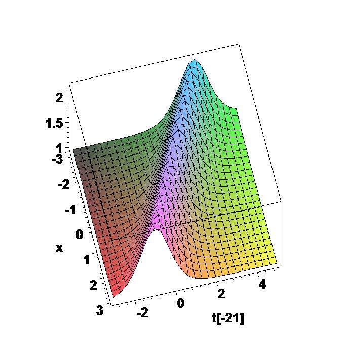
Bringing $\phi_{1}=\phi|_{z=z_{1}}$ in (4.19) into the above identities (4.15)-(4.18) will lead to specific form of the new solutions

$$u_{1}^{[1]} = (\Lambda^{2}-1)\frac{\cosh(\xi(x,t,z_{1}))+\cosh(\xi(x,t,\frac{1}{z_{1}}))}{\cosh(\xi(x-1,t,z_{1}))+\cosh(\xi(x-1,t,\frac{1}{z_{1}}))},$$

$$u_{0}^{[1]} = ((\Lambda^{2}-1)\frac{\cosh(\xi(x,t,z_{1}))+\cosh(\xi(x,t,\frac{1}{z_{1}}))}{\cosh(\xi(x-1,t,z_{1}))+\cosh(\xi(x-1,t,\frac{1}{z_{1}}))})$$

$$\times\frac{\cosh(\xi(x+1,t,z_{1}))+\cosh(\xi(x+1,t,\frac{1}{z_{1}}))}{\cosh(\xi(x,t,z_{1}))+\cosh(\xi(x,t,\frac{1}{z_{1}}))},$$

$$u_{-1}^{[1]} = ((\Lambda^{2}-1)\frac{\cosh(\xi(x,t,z_{1}))+\cosh(\xi(x,t,\frac{1}{z_{1}}))}{\cosh(\xi(x-1,t,z_{1}))+\cosh(\xi(x-1,t,\frac{1}{z_{1}}))})$$

$$\times\frac{\cosh(\xi(x+1,t,z_{1}))+\cosh(\xi(x+1,t,\frac{1}{z_{1}}))}{\cosh(\xi(x-1,t,z_{1}))+\cosh(\xi(x-1,t,\frac{1}{z_{1}}))},$$

$$u_{-2}^{[1]} = \frac{\cosh(\xi(x,t,z_{1}))+\cosh(\xi(x,t,\frac{1}{z_{1}}))}{\cosh(\xi(x-1,t,z_{1}))+\cosh(\xi(x-1,t,\frac{1}{z_{1}}))}\frac{\cosh(\xi(x-3,t,z_{1}))+\cosh(\xi(x-3,t,\frac{1}{z_{1}}))}{\cosh(\xi(x-2,t,z_{1}))+\cosh(\xi(x-2,t,\frac{1}{z_{1}}))},$$

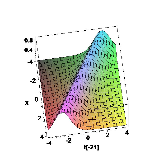
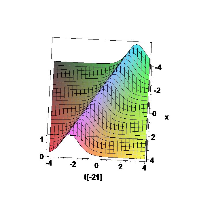
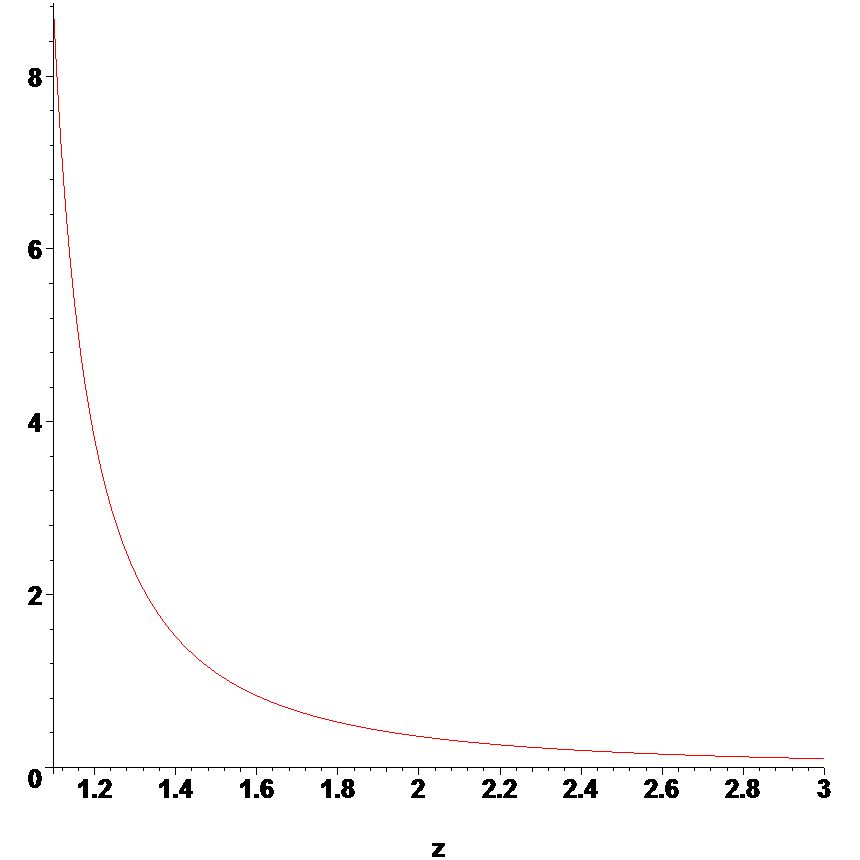
whose graphs are as Fig.1 in appendix.

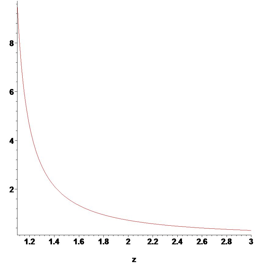
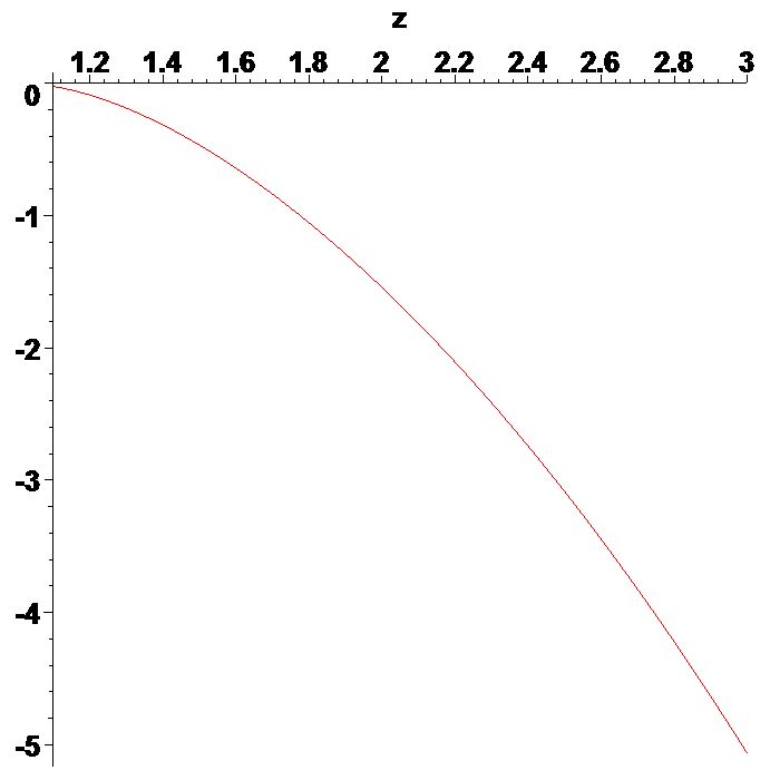
One can check that the new solutions satisfy primary flow equations (2.17),(2.19),(2.22),(4.1). For the above soliton solutions, we can find the velocity of the $t_{-2,1}$ flow is as $-\frac{(z^{2}+z^{-2})\log z+\frac{1}{2}(-z^{2}+z^{-2})}{\log z}$, the velocity of the $t_{0,0}$ flow is as $-\frac{z^{2}}{\log z}$ and the velocity of the $t_{1,0}$ flow is as $-\frac{z}{\log z}$. From Fig.2 in appendix, we can see the velocity of $t_{-2,1}$ flow which is quite different from the velocity of the $t_{0,0},t_{1,0}$ flow which can also be seen from the direction of the soliton graphs. When $z$ go to $+\infty$, the velocity becomes $-\infty$, which means the slop of the soliton will approach to be parallel to $x$ axis.

Obviously, the velocity of the extended flow is quite different from other flows. Of course, one can get higher order flows in the Lax equation eq.(4.1), i.e. $t_{\gamma,n},n\geq 1$ flows, the new higher-order soliton solutions and prove that the new solutions and other iterated n-soliton solutions can also satisfy them which will be not given in detail.

In the next section, it is time to introduce another Darboux transformation of the EBTH basing on another linear equation from eq.(2.24).

5. The second Darboux transformation of the EBTH

In fact the EBTH system can also be equivalently rewritten in form of the following linear differential system

$$\begin{cases}\mathcal{L}\psi&=\lambda\psi,\\ \frac{\partial\psi}{\partial t_{\alpha,n}}&=-(B_{\alpha,n})_{-}\psi,\ \alpha=N-1,N-2,\dots,-M,n\geq 0.\end{cases}$$ (5.1)

We will call the function $\psi$ in eq.(5.1) the second wave function of the EBTH.

In this section, we will consider the Darboux transformation of the EBTH on Lax matrix

$$\mathcal{L}=\Lambda^{N}+u_{N-1}\Lambda^{N-1}+\dots+u_{-M}\Lambda^{-M},$$ (5.2)

i.e.

$$\mathcal{L}^{[1]}=\Lambda^{N}+u_{N-1}^{[1]}\Lambda^{N-1}+\dots+u_{-M}^{[1]}\Lambda^{-M}=\bar{W}\mathcal{L}\bar{W}^{-1},$$ (5.3)

where $\bar{W}$ is Darboux transformation operator.

That means after Darboux transformation, the spectral problem

$$\mathcal{L}\psi=\Lambda^{N}\psi+u_{N-1}\Lambda^{N-1}\psi+\dots+u_{-M}\Lambda^{-M}\psi=\lambda\psi,$$ (5.4)

will become

$$\mathcal{L}^{[1]}\psi^{[1]}=\Lambda^{N}\psi^{[1]}+u_{N-1}^{[1]}\Lambda^{N-1}\psi^{[1]}+\dots+u_{-M}^{[1]}\Lambda^{-M}\psi^{[1]}=\lambda\psi^{[1]}.$$ (5.5)

To keep the Lax pair eq.(2.12) of the EBTH invariant, i.e.

$$\frac{\partial\mathcal{L}}{\partial t_{\alpha,n}}=[-(B_{\alpha,n})_{-},\mathcal{L}],\ \ \frac{\partial\mathcal{L}^{[1]}}{\partial t_{\alpha,n}}=[-(B_{\alpha,n}^{[1]})_{-},\mathcal{L}^{[1]}],\ \ B_{\alpha,n}^{[1]}:=B_{\alpha,n}(\mathcal{L}^{[1]}),$$ (5.6)

the dressing operator $\bar{W}$ should satisfy following dressing equation

$$\bar{W}_{t_{\gamma,n}}=\bar{W}(B_{\gamma,n})_{-}-(\bar{W}B_{\gamma,n}\bar{W}^{-1})_{-}\bar{W},\ \ -M\leq\gamma\leq N-1,n\geq 0.$$ (5.7)

Theorem 5.1.

If $\psi$ is the second wave function of the EBTH, the second Darboux transformation operator of the EBTH

$$\bar{W}(\lambda)=(\frac{\Lambda\psi}{\psi}-\Lambda)=\psi(x+\epsilon)\circ(1-\Lambda)\circ\psi^{-1}(x),$$ (5.8)

will generater new solutions $u_{i}^{[1]}$ from seed solutions $u_{i},-M\leq i\leq N-1$

$$u_{N-1}^{[1]} = \Lambda u_{N-1}+(\Lambda^{N}-1)\frac{\Lambda\psi}{\psi},$$ (5.9)

$$\dots \dots$$

$$u_{i}^{[1]} = \Lambda u_{i}+u_{i+1}^{[1]}(\Lambda^{i+1}\frac{\Lambda\psi}{\psi})-\frac{\Lambda\psi}{\psi}(\Lambda u_{i+1}),$$ (5.10)

$$\dots \dots,$$

$$u_{-M}^{[1]} = \frac{\Lambda\psi}{\psi}u_{-M}\frac{\Lambda^{-M}\psi}{\Lambda^{-M+1}\psi}.$$ (5.11)

Proof.

Using eq.(3.8) in Lemma 3.1, a direct computation will lead to the following

$$\bar{W}_{t_{\gamma,n}}\bar{W}^{-1} = (\psi(x+\epsilon)\circ(1-\Lambda)\circ\psi^{-1})_{t_{\gamma,n}}\psi\circ(1-\Lambda)^{-1}\circ\psi^{-1}(x+\epsilon)$$

$$= -(((B_{\gamma,n})_{-}\psi(x+\epsilon))\circ(1-\Lambda)\circ\psi^{-1})\psi\circ(1-\Lambda)^{-1}\circ\psi^{-1}(x+\epsilon)$$

$$+\psi(x+\epsilon)\circ(1-\Lambda)\circ((B_{\gamma,n})_{-}\psi)\psi^{-1}\circ(1-\Lambda)^{-1}\circ\psi^{-1}(x+\epsilon)$$

$$= -((B_{\gamma,n})_{-}\psi(x+\epsilon))\psi^{-1}(x+\epsilon)$$

$$+\psi(x+\epsilon)\circ(1-\Lambda)\circ((B_{\gamma,n})_{-}\psi)\psi^{-1}\circ(1-\Lambda)^{-1}\circ\psi^{-1}(x+\epsilon)$$

$$= -\psi(x+\epsilon)\circ[(\Lambda-1)\cdot(((B_{\gamma,n})_{-}\psi)\psi^{-1})]\Lambda\circ(1-\Lambda)^{-1}\circ\psi^{-1}(x+\epsilon)$$

$$= -(\psi(x+\epsilon)\circ[(\Lambda-1)\cdot(\psi^{-1}(B_{\gamma,n})_{-}\circ\psi)]\Lambda\circ(1-\Lambda)^{-1}\circ\psi^{-1}(x+\epsilon))_{+}$$

$$= \psi(x+\epsilon)\circ(1-\Lambda)\circ\psi^{-1}(x)\circ(B_{\gamma,n})_{-}(x)\circ\psi(x)\circ(1-\Lambda)^{-1}\circ\psi^{-1}(x+\epsilon)$$

$$-(\psi(x+\epsilon)\circ(1-\Lambda)\circ\psi^{-1}(x)\circ B_{\gamma,n}(x)\circ\psi(x)\circ(1-\Lambda)^{-1}\circ\psi^{-1}(x+\epsilon))_{-}$$

$$= \bar{W}(B_{\gamma,n})_{-}\bar{W}^{-1}-(\bar{W}B_{\gamma,n}\bar{W}^{-1})_{-}.$$

Therefore

$$\bar{W}=\psi(x+\epsilon)\circ(1-\Lambda)\circ\psi^{-1},$$ (5.12)

can be as another Darboux transformation of the EBTH. The new solutions can be got easily using the second dressing form eq.(5.3).

∎

Define $\psi_{i}=\psi_{i}^{[0]}:=\psi|_{\lambda=\lambda_{i}}$, then one can choose the specific one-fold Darboux transformation of the EBTH equations as following

$$\bar{W}_{1}(\lambda_{1})=\frac{\psi_{1}(x+\epsilon)}{\psi_{1}(x)}-\Lambda=\frac{\mathbb{T}_{1}}{\psi_{1}(x)},$$ (5.13)

where

$$\mathbb{T}_{1} = \left|\begin{matrix}1&\Lambda\\ \psi_{1}&\psi_{1}(x+\epsilon)\end{matrix}\right|.$$ (5.14)

Meanwhile, we can also get the Darboux transformation on wave function $\psi$ as following

$$\psi^{[1]}=(\frac{\Lambda\psi_{1}}{\psi_{1}}-\Lambda)\psi.$$ (5.15)

Then using iteration on Darboux transformation, the $j$-th Darboux transformation from the $(j-1)$-th solution is as

$$\psi^{[j]} = (\frac{\Lambda\psi_{j}^{[j-1]}}{\psi_{j}^{[j-1]}}-\Lambda)\psi^{[j-1]},$$ (5.16)

$$u_{N-1}^{[j]} = \Lambda u_{N-1}^{[j-1]}+(\Lambda^{N}-1)\frac{\Lambda\psi_{j}^{[j-1]}}{\psi_{j}^{[j-1]}},$$ (5.17)

$$\dots \dots$$

$$u_{i}^{[j]} = \Lambda u_{i-1}^{[j-1]}+u_{i+1}^{[j]}(\Lambda^{i+1}\frac{\Lambda\psi_{j}^{[j-1]}}{\psi_{j}^{[j-1]}})-\frac{\Lambda\psi_{j}^{[j-1]}}{\psi_{j}^{[j-1]}}u_{i+1}^{[j-1]},$$ (5.18)

$$\dots \dots,$$

$$u_{-M}^{[j]} = \frac{\Lambda\psi_{j}^{[j-1]}}{\psi_{j}^{[j-1]}}u_{-M}^{[j-1]}\frac{\Lambda^{-M}\psi_{j}^{[j-1]}}{\Lambda^{-M+1}\psi_{j}^{[j-1]}},$$ (5.19)

where $\psi_{i}^{[j-1]}:=\psi^{[j-1]}|_{\lambda=\lambda_{i}},$ are wave functions corresponding to different spectral with the $(j-1)$-th solutions $u_{N-1}^{[j-1]},u_{N-2}^{[j-1]},\dots,u_{-M}^{[j-1]}.$ It can be checked that $\psi_{i}^{[j-1]}=0,\ \ i=1,2,\dots,j-1.$

Theorem 5.2.

The two-fold Darboux transformation of the EBTH is as following

$$\bar{W}_{2}=t_{0}^{[2]}+t_{1}^{[2]}\Lambda+\Lambda^{2}=\frac{\mathbb{T}_{2}}{\Delta_{2}},$$ (5.20)

where

$$\Delta_{2}=\left|\begin{matrix}\psi_{1}(x)&\psi_{1}(x+\epsilon)\\ \psi_{2}(x)&\psi_{2}(x+\epsilon)\end{matrix}\right|,\ \ \mathbb{T}_{2} = \left|\begin{matrix}1&\Lambda&\Lambda^{2}\\ \psi_{1}&\psi_{1}(x+\epsilon)&\psi_{1}(x+2\epsilon)\\ \psi_{2}&\psi_{2}(x+\epsilon)&\psi_{2}(x+2\epsilon)\end{matrix}\right|.$$ (5.21)

The Darboux transformation leads to new solutions from seed solutions

$$u_{N-1}^{[2]} = \Lambda^{2}u_{N-1}-(\Lambda^{N}-1)t_{1}^{[2]},$$ (5.22)

$$\dots \dots,$$

$$u_{i}^{[2]} = \sum_{j=i}^{min{(N,i+2)}}u_{j}(x+(i+2-j)\epsilon)t_{i+2-j}^{[2]}-\sum_{j=i+1}^{min{(N,i+2)}}u_{j}^{[2]}t_{i+2-j}^{[2]}(x+j\epsilon),$$ (5.23)

$$\dots \dots,$$

$$u_{-M}^{[2]} = t_{0}^{[2]}(x)u_{-M}t_{0}^{[2]-1}(x-M\epsilon),$$ (5.24)

where $u_{i}^{[2]}$ can have another representation as

$$u_{i}^{[2]} = \frac{\sum_{j=max{(-M,i-2)}}^{i}u_{j}(x+(i-j)\epsilon)t_{i-j}^{[2]}-\sum_{j=max{(-M,i-2)}}^{i-1}u_{j}^{[2]}t_{i-j}^{[2]}(x+j\epsilon)}{t_{0}^{[2]}(x+i\epsilon)}.$$ (5.25)

Similarly, we can generalize the Darboux transformation to $n$-fold case which is contained in the following theorem.

Theorem 5.3.

The $n$-fold Darboux transformation of EBTH equation is as following

$$\bar{W}_{n}=t_{0}^{[n]}+t_{1}^{[n]}\Lambda+t_{2}^{[n]}\Lambda^{2}+\dots+(-1)^{n}\Lambda^{n}=\frac{1}{\Delta_{n}}\mathbb{T}_{n}$$ (5.26)

where

$$\Delta_{n} = \left|\begin{matrix}\psi_{1}(x)&\psi_{1}(x+\epsilon)&\psi_{1}(x+2\epsilon)&\dots&\psi_{1}(x+(n-1)\epsilon)\\ \psi_{2}(x)&\psi_{2}(x+\epsilon)&\psi_{2}(x+3\epsilon)&\dots&\psi_{2}(x+(n-1)\epsilon)\\ \psi_{3}(x)&\psi_{3}(x+\epsilon)&\psi_{3}(x+3\epsilon)&\dots&\psi_{3}(x+(n-1)\epsilon)\\ \vdots&\vdots&\vdots&\vdots&\vdots\\ \psi_{n}(x)&\psi_{n}(x+\epsilon)&\psi_{n}(x+3\epsilon)&\dots&\psi_{n}(x+(n-1)\epsilon)\\ \end{matrix}\right|$$

$$\mathbb{T}_{n} = \left|\begin{matrix}1&\Lambda&\Lambda^{2}&\Lambda^{3}&\dots&\Lambda^{n}\\ \psi_{1}(x)&\psi_{1}(x+\epsilon)&\psi_{1}(x+2\epsilon)&\psi_{1}(x+3\epsilon)&\dots&\psi_{1}(x+n\epsilon)\\ \psi_{2}(x)&\psi_{2}(x+\epsilon)&\psi_{2}(x+2\epsilon)&\psi_{2}(x+3\epsilon)&\dots&\psi_{2}(x+n\epsilon)\\ \psi_{3}(x)&\psi_{3}(x+\epsilon)&\psi_{3}(x+2\epsilon)&\psi_{3}(x+3\epsilon)&\dots&\psi_{3}(x+n\epsilon)\\ \vdots&\vdots&\vdots&\vdots&\vdots\\ \psi_{n}(x)&\psi_{n}(x+\epsilon)&\psi_{n}(x+2\epsilon)&\psi_{n}(x+3\epsilon)&\dots&\psi_{n}(x+n\epsilon)\\ \end{matrix}\right|.$$

The Darboux transformation leads to new solutions form seed solutions

$$u_{N-1}^{[n]} = \Lambda^{n}u_{N-1}+(-1)^{n}(1-\Lambda^{N})t_{n-1}^{[n]},$$ (5.27)

$$\dots \dots$$

$$u_{i}^{[n]} = \sum_{j=i}^{min{(N,i+n)}}u_{j}(x+(i+n-j)\epsilon)t_{i+n-j}^{[n]}-\sum_{j=i+1}^{min{(N,i+n)}}u_{j}^{[n]}t_{i+n-j}^{[n]}(x+j\epsilon),$$ (5.28)

$$\dots \dots,$$

$$u_{-M}^{[n]} = t_{0}^{[n]}(x)u_{-M}t_{0}^{[n]-1}(x-M\epsilon),$$ (5.29)

where $u_{i}^{[n]}$ can have another representation as

$$u_{i}^{[n]} = \frac{\sum_{j=max{(-M,i-n)}}^{i}u_{j}(x+(i-j)\epsilon)t_{i-j}^{[n]}-\sum_{j=max{(-M,i-n)}}^{i-1}u_{j}^{[n]}t_{i-j}^{[n]}(x+j\epsilon)}{t_{0}^{[n]}(x+i\epsilon)}.$$ (5.30)

It can be easily checked that $\bar{W}_{n}\psi_{i}=0,\ i=1,2,\dots,n.$

Taking seed solution $u_{N-1}=u_{N-2}=\dots=u_{-M+1}=0,u_{-M}=1$, then using Theorem 5.3, one can get the $n$-th new solution of the EBTH as

$$u_{N-1}^{[n]} = (-1)^{n}(1-\Lambda^{N})\partial_{t_{N-1,0}}\log Wr(\psi_{1},\psi_{2},\dots\psi_{n}),$$ (5.31)

$$\dots \dots$$

$$u_{-M}^{[n]} = e^{(\Lambda-1)(1-\Lambda^{-M})\log Wr(\psi_{1},\psi_{2},\dots\psi_{n})},$$ (5.32)

where $Wr(\psi_{1},\psi_{2},\dots\psi_{n})$ is the discrete Wronskian

$$Wr(\psi_{1},\psi_{2},\dots\psi_{n})=det(\Lambda^{j-1}\psi_{n+1-i})_{1\leq i,j\leq n}.$$ (5.33)

Particularly for the $(N,N)$-EBTH, choosing appropriate wave function $\psi$, another family of $n$-th new solutions can be solitary wave solutions, i.e. $n$-soliton solutions.

6. Another kind of soliton solutions

In this section, we will use the second Darboux transformation of the EBTH to generate a new kind of solutions from trivial seed solutions. In particular, when $N=M$, some soliton solutions will be shown using Darboux transformation.

To give a nice solution, one need to rewrite the extended flow in the Lax equations of the EBTH in the following form

$$\frac{\partial\mathcal{L}}{\partial t_{-M,n}}=[\bar{A}_{-M,n},\mathcal{L}],$$ (6.1)

$$\bar{A}_{-M,n}=-\frac{2}{\epsilon n!}[\mathcal{L}^{n}(\log\mathcal{L}-\frac{1}{2}(\frac{1}{M}+\frac{1}{N})c_{n})]_{-}+\frac{1}{\epsilon n!}[\mathcal{L}^{n}(\log_{+}\mathcal{L}-\frac{1}{2}(\frac{1}{M}+\frac{1}{N})c_{n})].$$ (6.2)

Taking seed solution $u_{N-1}=u_{N-2}=\dots=u_{-M+1}=0,u_{-M}=1$, then the initial wave function $\psi_{i}$ satisfies

$$\Lambda^{N}\psi_{i}+\Lambda^{-M}\psi_{i}=\lambda_{i}\psi_{i},\ 1\leq i\leq n.$$ (6.3)

To include all the dynamical variables, i.e. considering other flows in eq.(2.1) of the EBTH, wave function $\psi$ can be chosen in the form as

$$\psi =\sum_{m=1}^{N+M}a_{m}\exp(\frac{x+\frac{\lambda^{m}}{m!}t_{-M,m}}{\epsilon}\log z_{m}+\frac{t_{-M,m}}{2\epsilon m!}(\frac{1}{M}+\frac{1}{N})(-(\lambda^{m})_{+}+(\lambda^{m})_{-})-$$

$$\sum_{\alpha=1}^{N-1}\sum_{n\geq 0}\frac{\Gamma(2-\frac{\alpha}{N})}{\epsilon\Gamma(n+2-\frac{\alpha}{N})}(\lambda^{n+1-\frac{\alpha}{N}})_{-}t_{\alpha,n}-\sum_{\beta=-M+1}^{0}\sum_{n\geq 0}\frac{\Gamma(2+\frac{\alpha}{M})}{\epsilon\Gamma(n+2+\frac{\alpha}{M})}(\lambda^{n+1+\frac{\alpha}{M}})_{-}t_{\beta,n}),$$ (6.4)

where $z_{m}^{N}+z_{m}^{-M}=\lambda,\ 1\leq m\leq N+M,$ and the projection $``\pm"$ is about $z_{m}$. One can find the projection $(\lambda^{n+1+\frac{\alpha}{M}})_{+}$ now contains finite number of terms. Therefore this kind of Darboux transformation benefits in showing the character of the $t_{\beta,n},-M+1\leq\beta\leq 0$ flow. But one can find the projection $(\lambda^{n+1-\frac{\alpha}{N}})_{-}$ now contains infinite number of terms which tell us the second Darboux transformation is not so good to produce new solutions depending on $t_{\alpha,n},1\leq\alpha\leq N-1$. From this point, the extended bigraded Toda hierarchy is quite different from the extended Toda hierarchy[7]. Here the identity $z_{m}^{N}+z_{m}^{-M}=\lambda$ comes from eq.(6.3).

When $N=M$, we can choose $\psi$ as

$$\psi =\sum_{m=1}^{N}a_{m}cosh(\frac{x+\frac{\lambda^{m}}{m!}t_{-M,m}}{\epsilon}\log z_{m}+\frac{t_{-M,m}}{2\epsilon m!}(\frac{1}{M}+\frac{1}{N})(-(\lambda^{m})_{+}+(\lambda^{m})_{-})-$$

$$\sum_{\alpha=1}^{N-1}\sum_{n\geq 0}\frac{\Gamma(2-\frac{\alpha}{N})}{\epsilon\Gamma(n+2-\frac{\alpha}{N})}(\lambda^{n+1-\frac{\alpha}{N}})_{-}t_{\alpha,n}-\sum_{\beta=-M+1}^{0}\sum_{n\geq 0}\frac{\Gamma(2+\frac{\alpha}{M})}{\epsilon\Gamma(n+2+\frac{\alpha}{M})}(\lambda^{n+1+\frac{\alpha}{M}})_{-}t_{\beta,n}).$$ (6.5)

Then the new generated new solutions of the $(N,M)$-EBTH form trivial solutions using the wave function $\psi$ in eq.(6.4) are as

$$u_{N-1}^{[1]} = (\Lambda^{N}-1)\frac{\psi_{1}}{\Lambda\psi_{1}},$$ (6.6)

$$\dots \dots$$

$$u_{-M}^{[1]} = \frac{\Lambda\psi_{1}}{\psi_{1}}\frac{\Lambda^{-M}\psi_{1}}{\Lambda^{-M+1}\psi_{1}}.$$ (6.7)

The wave function $\psi$ in eq.(6.5) will be produced into one-soliton solution of the $(N,N)$-EBTH after transformation eq.(6.6)-eq.(6.7). Supposing $N=M=1$, the solutions will be exactly another kind of soliton solutions which are different from the soliton solutions mentioned in [11]. To see the solutions of the EBTH clearly, we will check the equations of $(2,2)$-EBTH, i.e. $N=M=2$ and prove the new kind of solutions after Darboux transformation are also solutions of the $(2,2)$-EBTH.

For the $(2,2)$-EBTH, to include all the dynamical variables, one can choose wave function $\psi$ in a form of a combination of

$$\psi =a\bar{\psi}(z)+b\bar{\psi}(\frac{1}{z}),$$ (6.8)

where

$$\bar{\psi} =\cosh(\frac{1}{\epsilon}\sum_{k\geq 0}[(x+\frac{\lambda^{k}t_{-2,k}}{k!})\log z+\frac{t_{-2,k}}{2k!}(-(\lambda^{k})_{+}+(\lambda^{k})_{-})]$$

$$-\sum_{\alpha=0}^{1}\sum_{n\geq 0}\frac{\Gamma(2-\frac{\alpha}{2})}{\epsilon\Gamma(n+2-\frac{\alpha}{2})}(\lambda^{n+1-\frac{\alpha}{2}})_{-}t_{\alpha,n}-\sum_{n\geq 0}\frac{\Gamma(2-\frac{1}{2})}{\epsilon\Gamma(n+2-\frac{1}{2})}(\lambda^{n+1-\frac{1}{2}})_{-}t_{-1,n}),$$ (6.9)

where $z^{2}+z^{-2}=\lambda,$ and the projection $\pm$ is about the powers of $z$. In the coefficients of $t_{1,n},t_{-1,n}$, the square roots of $\lambda$ mean the expansions around $\infty$ and $0$ respectively.

Then the soliton solution generated from eq.(6.8) is as

$$u_{1}^{[1]} = (\Lambda^{2}-1)\frac{\Lambda\psi_{1}}{\psi_{1}},$$ (6.10)

$$u_{0}^{[1]} = u_{1}^{[1]}(\Lambda\frac{\Lambda\psi_{1}}{\psi_{1}}),$$ (6.11)

$$u_{-1}^{[1]} = u_{0}^{[1]}(\frac{\Lambda\psi_{1}}{\psi_{1}}),$$ (6.12)

$$u_{-2}^{[1]} = \frac{\Lambda\psi_{1}}{\psi_{1}}\frac{\Lambda^{-2}\psi_{1}}{\Lambda^{-1}\psi_{1}}.$$ (6.13)

Choose $a=b=1,\epsilon=1$, then

$$\psi =\cosh(\xi(x,t,z))+\cosh(\xi(x,t,\frac{1}{z})),\ \$$ (6.14)

$$\xi(x,t,z) :=[(x+(z^{2}+z^{-2})t_{-2,1})\log z+\frac{t_{-2,1}}{2}(-z^{2}+z^{-2})]-z^{-2}t_{0,0}-z^{-1}t_{-1,0}.$$ (6.15)

Bringing $\psi_{1}=\psi|_{z=z_{1}}$ in (6.14) into the above identities (6.10)-(6.13) will lead to specific form of the new solutions

$$u_{1}^{[1]} = (\Lambda^{2}-1)\frac{\cosh(\xi(x+1,t,z_{1}))+\cosh(\xi(x+1,t,\frac{1}{z_{1}}))}{\cosh(\xi(x,t,z_{1}))+\cosh(\xi(x,t,\frac{1}{z_{1}}))},$$

$$u_{0}^{[1]} = ((\Lambda^{2}-1)\frac{\cosh(\xi(x+1,t,z_{1}))+\cosh(\xi(x+1,t,\frac{1}{z_{1}}))}{\cosh(\xi(x,t,z_{1}))+\cosh(\xi(x,t,\frac{1}{z_{1}}))})$$

$$\frac{\cosh(\xi(x+2,t,z_{1}))+\cosh(\xi(x+2,t,\frac{1}{z_{1}}))}{\cosh(\xi(x+1,t,z_{1}))+\cosh(\xi(x+1,t,\frac{1}{z_{1}}))},$$

$$u_{-1}^{[1]} = ((\Lambda^{2}-1)\frac{\cosh(\xi(x+1,t,z_{1}))+\cosh(\xi(x+1,t,\frac{1}{z_{1}}))}{\cosh(\xi(x,t,z_{1}))+\cosh(\xi(x,t,\frac{1}{z_{1}}))})$$

$$\frac{\cosh(\xi(x+2,t,z_{1}))+\cosh(\xi(x+2,t,\frac{1}{z_{1}}))}{\cosh(\xi(x,t,z_{1}))+\cosh(\xi(x,t,\frac{1}{z_{1}}))},$$

$$u_{-2}^{[1]} = \frac{\cosh(\xi(x+1,t,z_{1}))+\cosh(\xi(x+1,t,\frac{1}{z_{1}}))}{\cosh(\xi(x,t,z_{1}))+\cosh(\xi(x,t,\frac{1}{z_{1}}))}\frac{\cosh(\xi(x-2,t,z_{1}))+\cosh(\xi(x-2,t,\frac{1}{z_{1}}))}{\cosh(\xi(x-1,t,z_{1}))+\cosh(\xi(x-1,t,\frac{1}{z_{1}}))}.$$

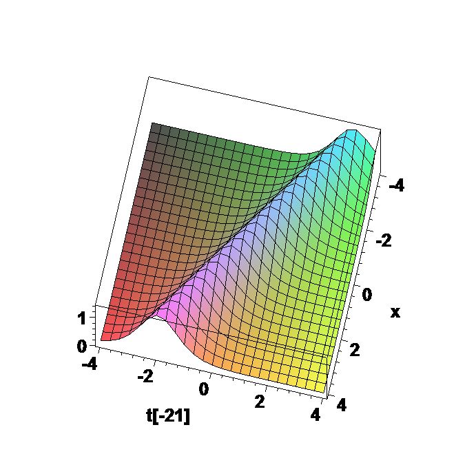
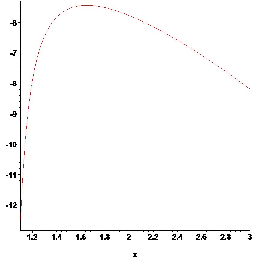
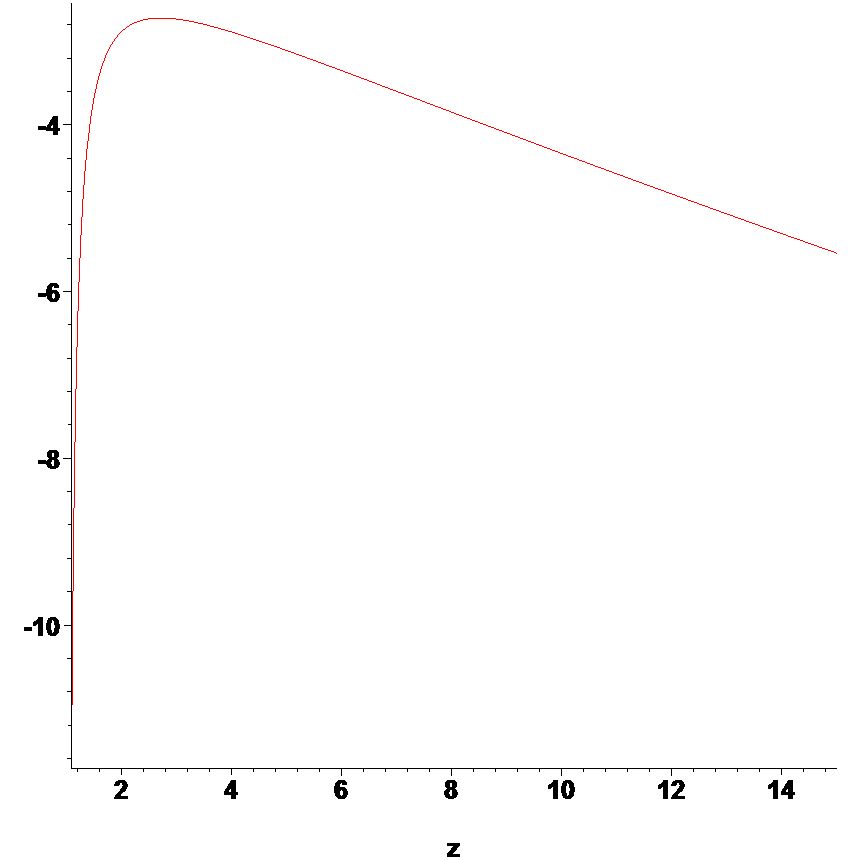
One can check that the new solutions satisfy primary flow equations (2.19),(2.21),(2.22),(6.1). For the above soliton solutions, we can find the velocity of the $t_{-2,1}$ flow is the same as the soliton solution generated from the first Darboux transformation, the velocity of the $t_{0,0}$ flow is as $\frac{1}{z^{2}\log z}$ and the velocity of the $t_{-1,0}$ flow is as $\frac{1}{z\log z}$. From Fig.3 in appendix, we can see the velocity of $t_{-2,1}$ flow which is quite different from the velocity of the $t_{0,0},t_{-1,0}$ flow which can also be seen from the direction of the soliton graphs. When $z$ go to $+\infty$, the velocity of the $t_{0,0},t_{-1,0}$ becomes $0$, which means the slop of the $t_{0,0},t_{-1,0}$ flow of the soliton flows will also approach to be vertical to $x$ axis.

7. Conclusions and Discussions

In this paper, we give two kinds of Darboux transformation of the EBTH which are used to generate new solutions from seed solutions including soliton solutions of $(N,N)$-EBTH. Meanwhile we plotted the soliton graphs of the $(N,N)$-EBTH from which some approximation analysis is done. From the analysis on velocities of soliton solutions, the effect of the extended flows are shown. Meanwhile the higher order Darboux transformation and the general form of the $n$-th new solutions are also given. It was found that the velocities of the extended flows are quite different from other flows. The application of these above two Darboux transformations in generating new solutions from known solutions related to the Gromov-Witten theory of orbiford $c_{NM}$ is an interesting questions. Also how to generate higher order solutions using the adjoint Darboux transformation and Binary Darboux transformation (see [23, 24]) of the EBTH and what the relation between the above two Darboux transformation in this paper and the adjoint and Binary Darboux transformation is are both interesting questions.

Acknowledgments. This work is supported by the Zhejiang Provincial Natural Science Foundation under Grant No. LY15A010004, the National Natural Science Foundation of China under Grant No. 11571192, the Natural Science Foundation of Ningbo under Grant No. 2015A610157 and the K. C. Wong Magna Fund in Ningbo University. The author would like to thank Professor J. S. He for his helpful suggestions.

Appendix:

($u_{1}^{[1]}$)  ($u_{0}^{[1]}$)  ($u_{-1}^{[1]}$)  ($u_{-2}^{[1]}$)

Figure 1. (color online)Soliton solution $u_{1}^{[1]},u_{0}^{[1]},u_{-1}^{[1]},u_{-2}^{[1]}$ of the $(2,2)$-EBTH when $z=2,a=b=1$ where the label $t[-21]$ is denoted as $t_{-2,1}$.

($v_{t_{-2,1}}$)  ($v_{t_{0,0}}$)  ($v_{t_{1,0}}$)

Figure 2. (color online)The velocity plot of the $t_{-2,1}$ flow, $t_{0,0}$ flow, $t_{1,0}$ flow of the soliton solution generated from the first Darboux transformation the $(2,2)$-EBTH.

($v_{t_{0,0}}$)  ($v_{t_{-1,0}}$)

Figure 3. (color online)The velocity plot of the $t_{0,0}$ flow, $t_{-1,0}$ flow of another soliton solution generated from the second Darboux transformation of the $(2,2)$-EBTH.