Impact of momentum anisotropy and turbulent chromo-fields on thermal particle production in quark-gluon plasma medium

Abstract

Momentum anisotropy present during the hydrodynamic evolution of Quark-Gluon Plasma (QGP) in RHIC may lead to chromo-Weibel instability and turbulent chromo-fields.The dynamics of the quark and gluon momentum distributions in this case is governed by an effective diffusive Vlasov equation (linearized). The solution of this linearized transport equation for the modified momentum distribution functions lead to the mathematical form of non-equilibrium momentum distribution functions of quarks/antiquarks and gluons. The modification to these distributions encode the physics of turbulent color fields and momentum anisotropy. In the present manuscript, we employ these distribution functions to to estimate thermal dilepton production rate in the QGP medium. The production rate is seen to have appreciable sensitivity to the strength of the anisotropy.

PACS: 25.75.-q; 24.85.+p; 05.20.Dd; 12.38.Mh

Keywords: Quark-Gluon Plasma; Momentum anisotropy Chromo-Weibel instability, Dilepton production; Quasi-particle model.

I Introduction

The experimental observation from the relativistic heavy-ion collisions at RHIC, BNL and LHC CERN, have strongly suggested the creation of quark-gluon-plasma (QGP) in a near perfect fluid state expt ; expt1 . The space time dynamics of the QGP has been modelled within the framework of second order relativistic dissipative hydrodynamics echo ; sch ; bozek ; review1 ; review2 ; song ; niemi . The hydrodynamical predictions for the collective flow coefficients and particle spectra in heavy-ion collisions (HIC), seen to work well for hadronic probes. The role of hydrodynamics in HIC has been to convert the geometrical fluctuations in the initial geometry of the reaction zone (soon after the collisions) to the momentum anisotropy, which finally leads to collective flow in the hadronic observables. Therefore, the momentum anisotropy has been there during the entire space-time evolution of the QGP. On the other hand, the early stages of the HIC where the momentum distribution is far from equilibrium and highly anisotropic, leading to instabilities has been well explored by several authors instab2-4 along with the detailed study on its consequences. For a very recent review, we refer readers to the Ref. strik_pr .

Based on the experimental observations, the QGP turned out to be a near perfect fluid with a tiny value for its shear viscosity to entropy ratio ($\eta/S\sim 1/{4\pi}$, which is smallest among almost all the known fluids in nature). It has been realized that collisional processes among effective gluonic and quark degrees of freedom of the QGP alone could not explain such a small number. The presence of momentum anisotropy is seen to play dominant role in in substantial modulation of shear viscosity of the hot QCD medium in weak coupling regime bmuller ; chandra_eta and may provide a possible explanation for the small, $\eta/S$. The main focus here is on the momentum anisotropy in the later stages of the collisions where the dynamics is governed by the hydrodynamics while the matter is near equilibrated. The physics of such momentum anisotropy is quite crucial to understand the QGP medium as in certain cases, it may lead to chromo-Weibel instability in the QGP chromoweibel and turbulent chromo-fields bmuller . As mentioned in peter , the fields generated by such instabilities help in rapid isotropization of the parton distributions and drive the system to hydrodynamical regime.

Instabilities have been extensively studied in the context of classical Yang-Mills dynamics and their role in thermalization and isotropization of the system strik_pr and their role in setting up the turbulence in the plasma. The two main frameworks for these investigations have been the classical-statistical lattice bergers12 ; bergers14 and CGC frameworks fukushima ; gelis . These classical-statistical lattice simulations bergers12 revealed that after an initial transient regime dominated by plasma instabilities and free streaming, the non-Abelian plasma exhibits the universal self-similar dynamics characteristic of wave turbulence. To handle the static case, Kurkela and Moore  kuk2012a proposed a new algorithm for solving the Yang-Mills equations in an expanding box that takes care of the transverse dynamics without getting affected by the longitudinal coarse lattices. The turbulence phenomenon has been studied in static box by Kurkela and Moore kukmo and Berges et al. bergers12 and they observed a cascade of energy flow towards higher momenta and existence of a scaling solution therein. On the other hand, the CGC lattice simulations by Fukushima fukushima and Fukushima and Gelis gelis have seen an energy flow from low to high wave number modes which eventually resulting in a spectrum consistent with Kolmogorov’s power law form indication of turbulent behavior. The later stages of longitudinally expanding plasmas after instabilities have stopped growing was studied by Berges et al. bergers14 where they highlighted the role of quantum fluctuations in the classical lattice simulations and their role in deciding the time scales for the system to isotropize and approache thermal equilibrium. From all these above studies and a few more (for details we refer the reader to strik_pr ), it is to be noted that the instabilities may lead to plasma turbulence. The role of instabilities and plasma turbulence might play crucial role in understanding the properties of the QGP in heavy-ion collisions while one concentrates on the anisotropy (momentum) in the later stages of the collisions.

The physics of the chromo-Weibel instability (non-Abelian analogue of Weibel instability weibel ) might play crucial role in understanding the space-time evolution and properties of QGP medium. The momentum anisotropy present during the hydrodynamic expansion of the QGP induces instability to the Yang-Mills field equations. The Weibel type of instabilities can be seen in the expanding QGP, since the width of the momentum component in the direction of the expansion squeezes by the expansion, leading to an anisotropic momentum distribution. The instability in the rapidly expanding QGP in heavy ion collisions may also lead to the plasma turbulence bmuller . Note that the plasma turbulence describes a random, non-thermal pattern of excitation of coherent color field modes in the QGP. The power spectrum, in this case, turns out to be similar to that of vortices in a turbulent fluid bmuller .

An effective transport equation (Vlasov-Boltzmann) has been setup in bmuller in a form applicable to the case of the turbulent QGP by making additional assumptions regarding the field distributions in the Vlasov term. To reflect the turbulent nature certain spatio-temporal correlation structure for fields at different space-time points (Gaussian form in bmuller ) has been considered. This allows one to rewrite the color-octet particle distribution function in the form of dissipative term acting on the singlet distribution and eventually leads to diffusive Vlasov-Boltzmann equation. Notably, the Vlasov (Force term) operator, thus, obtained in the effective transport equation only picks up the contributions from the anisotropy. The color electric field contribute through the thermal conductivity. The color-magnetic field mainly picks the anisotropy in the plasma medium. Here, we are only dealing with the latter. It has already been realized that such turbulent color fields, may contribute significantly to the transport processes in the QGP. As there is a significant decrease in the transport coefficients in the presence of turbulent fields dupree ; bmuller , the small shear viscosity to entropy ratio ($\eta/S$) can perhaps be understood in terms of the dominance of such fields.

The prime goal here is to investigate the dilepton production rate in the presence of chromo-Weibel instability. This could be done by first modeling the non-equilibrium momentum distribution functions vc_hq that describe expanding anisotropic QGP followed by employing it to the kinetic theory description of dilepton production in the QGP medium. Our formalism is a straightforward extension of the Ref. bmuller for the interacting/realistic hot QCD equation of state (here the (2+1)-flavor lattice EOS described in terms of a quasi-particle model). The hot QCD medium effects enter through the quasi-particle distribution functions along with the non-trivial energy dispersions. The near equilibrium quasi-quark and quasi-gluon distributions that are employed here are obtained earlier in vc_hq and utilized in the context of studying heavy-quark dynamics in the anisotropic QGP/QCD medium. In this work, we employ them in exploring the dilepton production from the thermal QGP medium following the kinetic theory description of the dilepton production by $q\bar{q}$ annihilation at leading order within (1+1)-d boost invariant expansion of the thermal QGP medium in longitudinal direction.

This is perhaps the first time, the impact of momentum anisotropy induced turbulent color fields has been included in the thermal particle production in hot QCD/QGP medium. As it will be seen in the later part of the manuscript that such effects indeed play significant role and can not simply be ignored for the momenta and temperatures accessible in RHIC. It is to be mentioned that such anisotropy induced momentum distributions have already been exploited to investigate the heavy-quark dynamics in the QGP medium  vc_hq . The heavy quark dynamics gets significant impact from such effects. Such effects may also be helpful to resolve the simultaneous estimation of $v_{2}$ and $R_{AA}$ for the heavy-quarks sdas .

Particles are produced from the thermal medium of expanding fireball created in heavy-ion collisions, throughout its evolution, carrying crucial information about the state of the constituent matter Alam:1996fd ; Alam:1999sc ; Peitzmann:2001mz ; vanHees:2007th . Effects of equation of states and non-equilibrium scenarios like dissipation etc. on such thermal particles from the QGP phase have been studied by various authors McLerran:1984ay ; Bhatt:2009zg ; Bhatt:2010cy ; PeraltaRamos:2010cw ; Bhatt:2011kx ; Bhalerao:2013aha ; Chandra:2015rdz . In this context it will be interesting to look how the presence of momentum anisotropy and turbulent chromo-fields will be affecting the thermal particle production.

The paper is organized as follows. In Section. II, the modeling of non-equilibrium distribution function in the presence of anisotropy driven instability has been presented. Section III, deals with the thermal particle productions rates in the anisotropic background medium and Section IV, discusses the yields in the presence of expanding medium in heavy-ion collisions. In section V, conclusions and outlook have been presented.

II Near (Non)-equilibrium quark and gluon distributions

Recall, the momentum anisotropy present in quark and gluon momentum distribution functions induces instability in the Yang-Mills equations in similar way as Weibel instability in the case of Electromagnetic plasmas. This instability while coupled with the rapid expansion of the QGP leads to anomalous transport and modulates the transport coefficients of the plasma substantially. This fact is realized by Dupree in the case of Electro-Magnetic plasmas in 1954 dupree and later generalized for the non-Abelian plasmas in Refs. bmuller ; chandra_eta1 . In the context of QGP, the phenomenon of the anomalous transport is realized at the later stages of the collisions, as due to the hydrodynamic expansion of the QGP, one has appreciable momentum anisotropy present in thermal distribution functions of quark and gluons.

To obtain the near equilibrium distribution within linearized transport theory we first need to have an adequate model for the isotropic (equilibrium) momentum distributions functions for the QGP degrees of freedom. To that end, we employ a quasi-particle description chandra_quasi of the lattice based QGP equation of state  cheng ; leos1_lat . In this model, form of the equilibrium distribution functions, $f_{eq}$ are obtained by encoding the strong interaction effects in terms of effective fugacities for quarks/gluons ($z_{g,q}$) as:

$$f_{0}^{g/q} = \frac{z_{g/q}\exp[-\beta E_{p}]}{\bigg{(}1\mp z_{g/q}\exp[-\beta E_{p}]\bigg{)}},$$

where $p=|\vec{p}|$, $E_{p}=p$ for gluons and light quarks ($u$ and $d$). On the other hand for strange quark in (2+1)-flavor QCD, $E_{p}=\sqrt{p^{2}+m_{s}^{2}}$ for (s-quarks). Here, $m_{s}$ denotes the mass of the strange quark, and $\beta=T^{-1}$ denotes inverse of the temperature. Since, the model is valid for temperatures that are higher than $T_{c}$, hence, we ignore the strange quark mass effects. The sub/superscript q denotes the $u$, $d$ and $s$ quarks. The effective fugacities ($z_{g/q}$) the model are not merely a temperature dependent parameters that encode the hot QCD medium effects; they lead to non-trivial dispersion relation both in the gluonic and quark sectors as,

$$\omega_{g,q} = E_{p}+T^{2}\partial_{T}ln(z_{g,q}).$$ (2)

For more detailed discussion on the understanding of $z_{g,q}$, we refer the reader to Ref. chandra_quasi . This quasi-particle description of hot QCD medium has seen to be highly useful in understanding the transport properties of hot QCD medium chandra_eta ; chandra_eta1 ; chandra_zeta , dilepton production in the QGP medium Chandra:2015rdz , electrical conductivity and charge diffusion in hot QCD medium chandra_sukanya .

It is worth to mention that there have been other quasi-particle descriptions in the literature, those could be characterized as, effective mass models  effmass1 ; effmass2 , effective mass models with gluon condensate effmass_glu , and effective models with Polyakov loop effective_pol ; effmass_pol . The effective model with Polyakov loop in effmass_pol has been thermodynamically consistent. The model employed here, is fundamentally distinct from all these models. In the presence of non-trivial quasi-particle dispersions (as in case of the say effective mass model or our model), the kinetic theory definition of energy-momentum tensor, $T^{\mu\nu}$ will get modified in terms of capturing the medium dependent terms jeon_yaffe ; blumn_1 ; dusling ; chandra_quasi . Such modifications are mandated by the fact that the $T^{\mu\nu}$ must incorporate the effects of trace anomaly. This fact in the case of effective mass models have been described and an effective $T^{\mu\nu}$ is obtained in Ref. blumn_1 . The authors further, estimated the viscosities of hot QCD matter blumn_1 . There has been more detailed study in this direction kapusta_pn . The mathematical expression for the modified $T^{\mu\nu}$ has been obtained for the current model in Ref. chandra_zeta . It is further to be noted that, Bluhm et al. blumn_2 , highlighted the utility of the effective mass models for the relativistic heavy ion collisions where non-zero baryon density aspects are also explored.

Next, we set-up an effective transport equation for the near-equilibrium momentum distribution functions for quarks and gluons in the presence of initial momentum anisotropy and space time expansion of the QGP.

II.1 An Effective kinetic equation–the Dupree-Vlasov equation

We start with the following ansatz for the non-equilibrium distribution function

$$f(\vec{p},\vec{r})=\frac{z_{g,q}\exp(-\beta u^{\mu}p_{\mu})}{1\pm z_{g,q}\exp\big{(}-\beta u^{\mu}p_{\mu}+f_{1}(\vec{p},\vec{r})\big{)}},$$ (3)

where $z_{g,q}$ are the effective gluon, quark fugacities coming from the isotropic modeling of the QGP in terms of lattice QCD equation of state and $u^{\mu}$ is the fluid 4-velocity considering fluid picture of the QGP medium. Here, $f_{1}(\vec{p},\vec{r})$ denotes the effects from the anisotropy (momentum) to the equilibrium distribution function. To achieve the above mentioned near equilibrium situation, $f_{1}$ must be a small perturbation. Under this condition, we obtain,

$$f(\vec{p},\vec{r})=f_{0}(p)+f_{0}(1\pm f_{0}(p))f_{1}(\vec{p},\vec{r})+O(f_{1}(\vec{p},\vec{r})^{2}).$$ (4)

The plus sign is for gluons and minus sign is for the quarks/antiquarks.

Next, the following form for the ansatz is considered for the linear order perturbation to the isotropic gluon and quarks distribution functions respectively,

$$f_{1}(\vec{p},\vec{r})=-\frac{1}{\omega_{g,q}T^{2}}\bigg{(}p_{i}p_{j}\Delta(\vec{p})(\nabla u)_{ij}\bigg{)},$$ (5)

where $f_{1}(\vec{p},\vec{r})\equiv f_{1}^{g,q}$ and $\Delta\equiv\Delta^{g,q}$. The quantity $\Delta$ captures effects from the momentum anisotropy. In the local rest frame of the fluid (LRF) $f_{0}=f_{eq}=(f_{0}^{g},f_{0}^{q})$, and considering longitudinal boost invariance Bjorken:1982qr , we obtain, $\nabla\cdot\vec{u}=\frac{1}{\tau}$ and ${\nabla u}_{ij}=\frac{1}{3\tau}diag(-1,-1,2)$, leading to

$$f_{1}^{g,q}=-\frac{\Delta^{g,q}(p)}{\omega_{g,q}T^{2}\tau}(p_{z}^{2}-\frac{p^{2}}{3}).$$ (6)

Let us now proceed to set up the effective transport equation in the presence of turbulent chromo-fields that are induced by the momentum anisotropy in the thermal distribution of the quasi-gluons and quarks while coupled with the rapid expansion of the QGP medium.

II.1.1 Effective transport equation in turbulent chromo fields

The near-equilibrium (anisotropic) momentum distributions for the quasi-gluons and quasi-quarks in our case were obtained by solving the Vlasov-Boltzmann equation in the presence of turbulent chromo fields in chandra_eta . The approach has been based on a straightforward extension of the work Asakawa et. al,  bmuller . Below, we offer the essential steps in the determination of the distributions.

The evolution of the quasi-quark and quasi-gluon momentum distribution functions in the anisotropic QGP medium with color fields can be obtained by setting up Vlasov-Boltzmann equation Heinz:1983nx as:

$$v^{\mu}\frac{\partial}{\partial x^{\mu}}f({\bf r},{\bf p},t)+g{\bf F}^{a}\cdot\nabla_{q}f^{a}({\bf r},{\bf p},t)=0\,$$ (7)

where $f({\bf r},{\bf q},t)$ represent the parton distribution in phase space (sums over all parton colors), the quantities ${\bf p}\equiv\vec{p}$ and ${\bf r}\equiv\vec{r}$. Here, $f^{a}({\bf r},{\bf q},t)$ denotes the color octet distribution function. Note that, here we are dealing with the collisionless plasma. Both the distributions, $f$ and $f^{a}$ are defined in the semi-classical formalism in Ref. Heinz:1984yq as the moments of the distribution function ${\tilde{f}}({\bf r},{\bf p},Q,t)$ in an extended phase space that includes the color sector as:

$$f({\mathbf{r}},{\bf p},t) = \int dQ\,{\tilde{f}}({\bf r},{\bf p},Q,t)\,,$$ (8)

$$f^{a}({\mathbf{r}},{\bf p},t) = \int dQ\,Q^{a}{\tilde{f}}({\bf r},{\bf p},Q,t)\,.$$ (9)

Here $Q^{a}$ denotes the color charge, $v^{\mu}=\frac{p^{\mu}}{p^{0}}$, $p^{\mu}=(p^{0}=E_{p},\vec{p})$. The color Lorentz force is defined as:

$${\bf F}^{a}=E^{a}+{\bf v}\times B^{a}.$$ (10)

The color octet distribution function, $f^{a}$ will satisfy a transport equation which involve coupling with the phase space distributions of higher color-SU(3) representations. The near equilibrium considerations allows us to truncate this hierarchy by keeping only the lowest order term in the gradients for both $f$ and $f^{a}$. The color octet distribution identically vanishes at equilibrium. This implies that it is at least linear in perturbation. With these consideration, the transport equation for $f^{a}$ is obtained as  Heinz:1983nx ; Heinz:1984yq :

$$v^{\mu}\frac{\partial f^{a}}{\partial x^{\mu}}+gf_{abc}A^{b}_{\mu}v^{\mu}f^{c}+\frac{gC_{2}}{N_{c}^{2}-1}{\bf F}^{a}\cdot\nabla_{p}f=0,$$ (11)

where $C_{2}$ and $f_{abc}$ represent quadratic Casimir invariant ($C_{2}\equiv\big{(}N_{c},(N_{c}^{2}-1)/{2N_{c}}\big{)}$ and structure constants of the $SU(N_{c})$ respectively, and $A^{\mu}$ represents the gauge field.

Now the goal is to solve Eq.(11) and obtain $f^{a}$ in terms of $f$ and finally solve Eq.(7), in the case of turbulent Chromo fields. This has been done in bmuller treating isotropic hot QCD/QGP as the ultra-relativistic gas of the quarks-antiquarks and gluons. In our case, the isotropic (local equilibrium) state is described in terms of effective quasi-gluon and quasi-quarks/antiquarks that describes the realistic hot QCD EOS (lattice) in the local rest frame of the QGP fluid. The extension of the whole treatment to the present case turned out to be quite straightforward. The interactions enter through the distribution functions and modified energy dispersions chandra_eta .

Following bmuller ; chandra_eta , we obtain an effective diffusive Vlasov-Boltzmann equation for the turbulent fields:

$$v^{\mu}\frac{\partial}{\partial x^{\mu}}\bar{f}-{\mathcal{F}_{V}}\bar{f}=0\,.$$ (12)

where,

$${\mathcal{F}_{V}} = -\frac{g^{2}C_{2}}{4(N_{c}^{2}-1)\omega_{g,q}^{2}}\langle E^{2}+B^{2}\rangle\,\tau_{\rm m}$$ (13)

$$\times\left[({\mathbf{L}}^{(p)})^{2}-(L^{(p)}_{z})^{2}\right]\,$$

Here, $-i{\mathbf{p}}\times\nabla_{p}={\mathbf{L}}^{(p)}$, ${\bf v}={\bf p}/\omega_{g,q}$ and for the $\bar{f}(\vec{p})$ we shall employ $f(\vec{p})$ in Eq.(II). Here, $\bar{f}$ denotes the ensemble averaged momentum distribution (singlet) function of quasi-partons bmuller . In our case, $\bar{f}\equiv f(\vec{p},\vec{r})$, as given in Eq. (3). Note that we are only considering the anomalous transport and the collision term is not taken in to account here. The argument here is based on the fact that the anomalous transport process, which leads to highly significant suppression of the transport coefficients in the expanding QGP, is the dominant mechanism to understand the tiny value of the $\eta/S$ for the QGP. We intend to revisit it, employing an appropriate collision term in the near future. In obtaining the above mentioned diffusive Vlasov equation, appropriate forms correlation functions functions (Gaussian correlators satisfy all the assumptions) for the color fields have been chosen bmuller while assuming that the color-electric and -magnetic field are uncorrelated. Being real and symmetry properties of the Gaussian correlators with respect to two space-time points express the chaotic nature of the hot QCD plasma. This is how the turbulent nature of the plasma and its effects on the dynamics through the transport equation is introduced here, following Ref.bmuller .

The force term (${\mathcal{F}_{V}}$) in the case of chromo-electromagnetic plasma will have the following form bmuller :

$${\mathcal{F}_{V}}\bar{f}(p) \equiv{\mathcal{F}_{V}}f(\vec{p},\vec{r})$$ (14)

$$= \frac{g^{2}C_{2}}{3(N_{c}^{2}-1)\omega^{2}_{g,q}}\langle E^{2}+B^{2}\rangle\tau_{m}$$

$$\times[({\mathbf{L}}^{(p)})^{2}-(L^{(p)}_{z})^{2}]f_{eq}(1\pm f_{eq})p_{i}p_{j}(\nabla u)_{ij}.$$

The quantities $\langle E^{2}\rangle$ and $\langle B^{2}\rangle$ are the color averaged chromo-electric and chromo-magnetic fields (average over the ensemble of turbulent color fields bmuller ), $\tau_{m}$ is the time scale for the instability.

Now, the action of the drift operator on $f_{eq}$ is given by:

$$(v\cdot\partial)f_{eq} = -f_{eq}(1+f_{eq})\bigg{\{}(p-\partial_{\beta}\ln(z_{g,q}))v\cdot\partial(\beta)$$ (15)

$$+\beta(v\cdot\partial)(u\cdot p)\bigg{\}},$$

where, $p-\partial_{\beta}\ln(z_{g/q})\equiv\omega_{g,q}$, is the modified dispersion relations. After some mathematical massaging, we obtain the following expression for the drift term,

$$(v\cdot\partial)f_{eq}(p) = f_{eq}(1\pm f_{eq})\bigg{[}\frac{p_{i}p_{j}}{\omega_{g,q}T}(\nabla u)_{ij}$$

$$-\frac{m^{2}_{D}\langle E^{2}\rangle\tau^{el}\omega_{g,q}}{3T^{2}{\partial{\varepsilon}}/{\partial T}}$$

$$+(\frac{p^{2}}{3\omega_{g,q}^{2}}-c^{2}_{s})\frac{\omega_{g,q}}{T}(\nabla\cdot\vec{u})\bigg{]},$$

where $c^{2}_{s}$ is the speed of sound, $m^{2}_{D}$ is the Debye mass, ${\varepsilon}$ is the energy density, $\tau_{el}$ is the time scale of the instability in chromo-electric fields. The expression is mathematically similar to bmuller . The only difference is the appearance of modified quasi-particle dispersion.

Finally, the effective Vlasov-Dupree equation (linearized) in the presence of turbulent color fields with the above ansatz is formulated in Refs. bmuller ; chandra_eta reads:

$$\bigg{\{}(\frac{p^{2}}{3\omega_{g,q}}-c_{s}^{2})\frac{\omega_{g,q}}{T}(\nabla\cdot\vec{u})+\frac{p_{i}p_{j}(\nabla u)_{ij}}{\omega_{g,q}T}\bigg{\}}f_{0}^{g,q}(1\pm f_{0}^{g,q})=$$

$$\frac{g^{2}C_{2}}{3(N_{c}^{2}-1)\omega^{2}_{g,q}}\langle E^{2}+B^{2}\rangle\tau_{m}{\mathcal{L}}^{2}f_{1}^{g,q}(\vec{p})f_{0}^{g,q}(1\pm f_{0}^{g,q}).$$ (17)

Importantly, first term in the left hand side of Eq.(II.1.1) contributes to the physics of isotropic expansion (bulk viscosity effects) which is not taken into account in the present work. As the analysis is valid for temperatures which are away from $T_{c}$, the bulk viscous effects can conveniently be neglected there.

Next, solving Eq. (II.1.1) for $\Delta$ analytically, we obtain the following expression chandra_zeta ,

$$\Delta(\vec{p}) = 2(N_{c}^{2}-1)\frac{\omega_{g,q}T}{3C_{2}g^{2}\langle E^{2}+B^{2}\rangle_{g,q}\tau_{m}}.$$ (18)

The unknown factor, $\langle E^{2}+B^{2}\rangle_{g,q}\tau_{m}$ in the denominator of Eq. (18) can be related to the phenomenologically known quantity the jet quenching parameter, $\hat{q}$, in both gluonic and quark sectors as done in Ref. majumder . This connection is established as mentioned below. The two crucial transport coefficients that may get significant contribution from the turbulent color fields are shear viscosity, $\eta$ and jet quenching parameter, $\hat{q}$. Thus, the strength of momentum anisotropy in the expanding QGP medium can be related to the physics of these parameters. Recall that the strength of the anisotropy, $\Delta(\vec{p})$ is related to the $\eta$. The coefficient, $\eta$ is seen to be inversely proportional to the $\hat{q}$ bmuller ; chandra_eta . The jet quenching parameter, $\hat{q}$ turns out to be proportional to the mean momentum square per unit length on the an energetic parton imparted by turbulent fields ask:2010 . In that context the anisotropy is related to the quenching. Here, we relate the unknown quantities $\langle E^{2}+B^{2}\rangle\tau_{m}$- which encodes the physics of anisotropy and chromo-Weibel instability, to the $\hat{q}$ both in gluonic and matter sectors as majumder

$$\hat{q}=\frac{2g^{2}C_{g/f}}{3(N_{c}^{2}-1)}\langle E^{2}+B^{2}\rangle\tau_{m},$$ (19)

where $C_{g}=N_{c}$, $C_{f}=\frac{(N_{c}^{2}-1)}{2N_{c}}$ for the gluons and quarks respectively. In the present case, we have $N_{c}=3$.

Employing the definition of $\hat{q}$ from Eq. (19) in Eq. (18), we obtain the following expression for the $\Delta$ term,

$$\Delta = \frac{4\omega_{g,q}^{2}T}{9\hat{q}_{g,q}}$$

With the above relation, we obtain the near equilibrium distribution functions in terms of the jet quenching parameter $\hat{q}$ as,

$$f^{g,q}(\vec{p}) = f_{0}^{g,q}-f_{0}^{g,q}(1\pm f_{0}^{g,q})\frac{4\omega_{g,q}}{9\hat{q}_{g,q}T\tau}\big{(}p_{z}^{2}-\frac{p^{2}}{3}\big{)}.$$ (21)

The jet quenching parameter, $\hat{q}$ for both gluons and quarks has been estimated phenomenologically within several different approaches burke ; 55 ; 50 ; 51 ; 56 ; 42 . The gluon quenching parameter $\hat{q}_{g}$ can be obtained from the relation, $\hat{q}_{g}\equiv\frac{9}{4}$ (in terms of Casimir invariants of the $SU(3)$ group). As we shall see later, such values of $\hat{q}_{g,q}$ induce very strong non-perturbative effects to the dileptons spectra.

It is to be noted that we have only three independent functions ($z_{g}$, $z_{q}$, and $\hat{q}$) ($\hat{q}$ for gluons and quarks are related by the respective Casimirs of $SU(3)$). The first two functions are estimated while describing the hot QCD equation of state. As stated earlier, the third one is a phenomenological parameter. Let us now proceed to investigate the thermal particle rates in the QGP medium.

It is important to note that momentum anisotropy and plasma instabilities in the initial stages of the RHIC have extensively been studied in the literature by several authors while investigating the effects of color collective excitations smrow and thermalization arnold1 there. Rebhan et. al,  rebhan studied the dynamics of non-abelian plasma instabilities within Hard-loop dynamics and Romatschke and Venugopalan venu explored the same within CGC framework. The collective plasma modes in anisotropic QGP have been studied in roma1 ; carrig ; chandra_ins . The collisional energy loss in anisotropic QGP roma2 , the momentum broadening roma3 , the radiative energy loss roy , and the wake potential wake are some of the related effects those have been investigated in the anisotropic QGP. For recent reviews, we refer the reader to Refs. strik_pr ; rev1 and references therein.

III Modified Thermal particle rates in QGP

Particles are produced in all stages during fireball evolution in the heavy-ion collisions from locally thermalized QGP medium. The main focus here is to investigate dilepton pair in the thermal QGP medium via $q\bar{q}$ -annihilation (most dominant source of dilepton pair production). As discussed in detail earlier, the momentum anisotropy present during the hydrodynamic evolution of the QGP medium in RHIC can be captured as the modification in the equilibrium (local) distributions of the gluonic and quark-antiquark degrees of freedom by setting up and solving an appropriate Vlasov-Boltzmann equation (linearized). The linear approximation is valid while the modifications are much smaller as compared to their equilibrium counterpart. In this near equilibrium situation, we can still utilize the kinetic theory for obtaining particle production rates and yields. This could be done by just replacing the expressions for the momentum distributions as the modified ones as done below.

The major source of thermal dileptons in the QGP medium is the $q\bar{q}$ annihilation process, $q\bar{q}\rightarrow\gamma^{*}\rightarrow l^{+}l^{-}$. Rate of dilepton production for this process can be written as rvogt :

$$\frac{dR}{d^{4}p}^{\tiny{l^{+}l^{-}}} = \int\left[gf(\vec{p}_{1})\frac{d^{3}\vec{p}_{1}}{(2\pi)^{3}}\right]\left[gf(\vec{p}_{2})\frac{d^{3}\vec{p}_{2}}{(2\pi)^{3}}\right]$$ (22)

$$\times\sigma(M^{2})\,v_{rel}\,\delta^{4}(p-p_{1}-p_{2}).$$

Here $p=(E=E_{1}+E_{2},\,\vec{p}=\vec{p}_{1}+\vec{p}_{2})$ is the four momentum of the dileptons and $p_{1(2)}=(E_{1(2)},\vec{p}_{1(2)})$ is that of quark or anti-quark with $E_{1(2)}\simeq|\vec{p}_{1(2)}|$, while neglecting the quark masses. We denote the invariant mass of the virtual photon as $M^{2}=(E_{1}+E_{2})^{2}-(\vec{p}_{1}+\vec{p}_{2})^{2}$. The relative velocity of the quark-anti-quark pair is given by $v_{rel}=\sqrt{\frac{M^{2}(M^{2}-4m_{q}^{2})}{4E_{1}^{2}E_{2}^{2}}}\simeq\frac{M^{2}}{2E_{1}E_{2}}$ and the term $\sigma(M^{2})$ is the relevant thermal dilepton production cross section. With $N_{f}$=2 and $N_{c}=3$, we have $M^{2}g^{2}\sigma(M^{2})=\frac{80\pi}{9}\alpha^{2}$ Alam:1996fd . The functions $f(\vec{p})$ are the quark and anti-quark distribution functions with $g$ being the corresponding degeneracy factor. The expressions for quark and antiquark distribution functions are obtained in the previous section, have the expressions:

$$f(\vec{p})=f_{0}-f_{0}(1-f_{0})\frac{4\omega_{q}}{9\hat{q}_{q}T}\big{(}p_{i}p_{j}\Delta u_{ij}\big{)}.$$ (23)

Since, we are interested in large invariant mass regime $M\gg T\gg m_{q}$, we can approximate, Fermi-Dirac distribution by classical Maxwell-Boltzmann distribution, so that

$$f_{0}(\vec{p_{i}}) \approx z_{q}e^{-E_{i}/T}$$

$$f(\vec{p_{i}}) \approx z_{q}e^{-E_{i}/T}\left[1-\frac{4\omega_{q}}{9\hat{q}_{q}T}\big{(}p_{i}p_{j}\Delta u_{ij}\big{)}\right].$$ (24)

Keeping only up to the quadratic order in momenta, we can write the dilepton production rate asBhatt:2011kx ,

$$\frac{dR}{d^{4}p}^{\tiny{l^{+}l^{-}}} = \int\frac{d^{3}\vec{p}_{1}}{(2\pi)^{3}}\frac{d^{3}\vec{p}_{2}}{(2\pi)^{3}}\frac{M^{2}g^{2}\sigma(M^{2})}{2E_{1}E_{2}}\delta^{4}(p-p_{1}-p_{2})$$ (25)

$$\times f_{0}(\vec{p_{1}})f_{0}(\vec{p_{2}})\left[1-2\,\frac{4\omega_{q}}{9\hat{q}_{q}T}\big{(}{p_{1}}_{i}{p_{1}}_{j}\Delta u_{ij}\big{)}\right]$$

$$= \frac{dR_{0}}{d^{4}p}^{\tiny{l^{+}l^{-}}}+\,\frac{dR_{1}}{d^{4}p}^{\tiny{l^{+}l^{-}}}.$$

The equilibrium contribution to the dilepton production

$$\frac{dR_{0}}{d^{4}p}^{\tiny{l^{+}l^{-}}} = \int\frac{d^{3}\vec{p}_{1}}{(2\pi)^{6}}~{}\frac{M^{2}g^{2}\sigma(M^{2})}{2E_{1}E_{2}}\delta(E-E_{1}-E_{2})$$ (26)

$$\times~{}z_{q}^{2}e^{-(E_{1}+E_{2})/T}$$

is known and is given byChandra:2015rdz

$$\frac{dR_{0}}{d^{4}p}^{\tiny{l^{+}l^{-}}} = \frac{z_{q}^{2}}{2}~{}\frac{M^{2}g^{2}\sigma(M^{2})}{(2\pi)^{5}}~{}e^{-E/T}.$$ (27)

Next, we calculate the non-equilibrium contribution to dilepton production, given as

$$\frac{dR_{1}}{d^{4}p}^{\small{l^{+}l^{-}}} = -2\int\frac{d^{3}\vec{p}_{1}}{(2\pi)^{6}}~{}\frac{M^{2}g^{2}\sigma(M^{2})}{2E_{1}E_{2}}\delta(E-E_{1}-E_{2})$$ (28)

$$~{}~{}~{}~{}\times~{}z_{q}^{2}e^{-(E_{1}+E_{2})/T}\left[\frac{4\omega_{q}}{9\hat{q}_{q}T}\big{(}{p_{1}}_{i}{p_{1}}_{j}\Delta u_{ij}\big{)}\right]$$

$$= I_{ij}(p)\Delta u_{ij}.$$

Here we have represented

$$I_{ij}(p) = -2\int\frac{d^{3}\vec{p}_{1}}{(2\pi)^{6}}~{}\frac{M^{2}g^{2}\sigma(M^{2})}{2E_{1}E_{2}}\delta(E-E_{1}-E_{2})$$ (29)

$$~{}~{}~{}~{}\times~{}z_{q}^{2}e^{-(E_{1}+E_{2})/T}\frac{4\omega_{q}}{9\hat{q}_{q}T}{p_{1}}_{i}{p_{1}}_{j}.$$

Now, the most general form of this second rank tensor in LRF can be written as,

$$I_{ij}(p)=a_{0}~{}\delta_{ij}+a_{2}~{}p_{i}p_{j}.$$ (30)

However, we note that on contraction with $\Delta u_{ij}$ only $a_{2}$ will survive as $\delta_{ij}\Delta u_{ij}=0$. By constructing projection operator $Q_{ij}$ we can calculate $a_{2}=Q_{ij}I_{ij}$, where form of the projection operator in LRF is given by

$$Q_{ij}=-\frac{1}{2|{\vec{p}}|^{2}}\left(\delta_{\ij}-\frac{3p_{i}p_{j}}{|{\vec{p}}|^{2}}\right).$$ (31)

Now, the expression for non-equilibrium contribution to dilepton rate becomes,

$$\frac{dR_{1}}{d^{4}p}^{\small{l^{+}l^{-}}} = I_{ij}(p)\Delta u_{ij}=\left[Q_{mn}I_{mn}\right]p_{i}p_{j}\Delta u_{ij}.$$ (32)

Computations of $Q_{mn}I_{mn}$ can be done using Eq.(29) and Eq.(31),

$$Q_{mn}I_{mn} = -2\int\frac{d^{3}\vec{p}_{1}}{(2\pi)^{6}}~{}\frac{M^{2}g^{2}\sigma(M^{2})}{2E_{1}E_{2}}\delta(E-E_{1}-E_{2})$$ (33)

$$~{}~{}~{}~{}\times~{}z_{q}^{2}e^{-(E_{1}+E_{2})/T}\frac{4\omega_{q}}{9\hat{q}_{q}T}{p_{1}}_{m}{p_{1}}_{n}$$

$$~{}~{}~{}~{}\times\left[-\frac{1}{2|{\vec{p}}|^{2}}\left(\delta_{mn}-\frac{3p_{m}p_{n}}{|{\vec{p}}|^{2}}\right)\right]$$

$$= -\frac{8}{9}\frac{1}{\hat{q}_{q}T}\int\frac{d^{3}\vec{p}_{1}}{(2\pi)^{6}}~{}\frac{M^{2}g^{2}\sigma(M^{2})}{2E_{1}E_{2}}\delta(E-E_{1}-E_{2})$$

$$~{}~{}~{}~{}~{}~{}~{}~{}~{}~{}\times~{}z_{q}^{2}e^{-(E_{1}+E_{2})/T}\{p_{1}+T^{2}\partial_{T}\,ln(z_{q})\}$$

$$~{}~{}~{}~{}~{}~{}~{}~{}~{}~{}\times\left[-\frac{|{\vec{p_{1}}}|^{2}}{2|{\vec{p}}|^{2}}+\frac{3(\vec{p}\cdot\vec{p_{1}})}{2|{\vec{p}}|^{4}}\right]$$

$$= -\frac{8}{9}\frac{1}{\hat{q}_{q}T}\left[\mathscr{M}+\mathscr{N}\right],$$

where we have used Eq.(2): $\omega_{q}=p+T^{2}\partial_{T}\,ln(z_{q})$. Next, we calculate integrals $\mathscr{M}$ and $\mathscr{N}$, and they are found to be

$$\mathscr{M} = \int\frac{d^{3}\vec{p}_{1}}{(2\pi)^{6}}~{}\frac{M^{2}g^{2}\sigma(M^{2})}{2E_{1}E_{2}}\delta(E-E_{1}-E_{2})$$ (34)

$$\times~{}z_{q}^{2}e^{-(E_{1}+E_{2})/T}\{p_{1}\}\left[-\frac{|{\vec{p_{1}}}|^{2}}{2|{\vec{p}}|^{2}}+\frac{3(\vec{p}\cdot\vec{p_{1}})}{2|{\vec{p}}|^{4}}\right]$$

$$= \frac{E}{4}~{}\frac{dR_{0}}{d^{4}p}^{\tiny{l^{+}l^{-}}}$$

and

$$\mathscr{N} = \int\frac{d^{3}\vec{p}_{1}}{(2\pi)^{6}}~{}\frac{M^{2}g^{2}\sigma(M^{2})}{2E_{1}E_{2}}\delta(E-E_{1}-E_{2})$$ (35)

$$\times~{}z_{q}^{2}e^{-(E_{1}+E_{2})/T}\{T^{2}\partial_{T}\,ln(z_{q})\}\left[-\frac{|{\vec{p_{1}}}|^{2}}{2|{\vec{p}}|^{2}}+\frac{3(\vec{p}\cdot\vec{p_{1}})}{2|{\vec{p}}|^{4}}\right]$$

$$= \frac{1}{3}~{}T^{2}\partial_{T}\,ln(z_{q})~{}\frac{dR_{0}}{d^{4}p}^{\tiny{l^{+}l^{-}}}.$$

Non-equilibrium contribution to dilepton rates can be written using Eq.(33) and Eq.(32) as

$$\frac{dR_{1}}{d^{4}p}^{\small{l^{+}l^{-}}} = -\frac{8}{9}\frac{1}{\hat{q}_{q}T}\left[\frac{E}{4}+\frac{1}{3}T^{2}\partial_{T}\,ln(z_{q})\right]$$ (36)

$$\times\frac{dR_{0}}{d^{4}p}^{\tiny{l^{+}l^{-}}}p_{i}p_{j}\Delta u_{ij}.$$

Finally, we write the expression for total dilepton production, using Eq.(25) as

$$\frac{dR}{d^{4}p}^{\small{l^{+}l^{-}}} = \left[1-\frac{8}{9}\frac{1}{\hat{q}_{q}T}\left(\frac{E}{4}+\frac{1}{3}~{}T^{2}\partial_{T}\,ln(z_{q})\right)p_{i}p_{j}\Delta u_{ij}\right]$$ (37)

$$\times\frac{dR_{0}}{d^{4}p}^{\tiny{l^{+}l^{-}}}.$$

Next, we plot the equilibrium rates $\frac{dR_{0}}{d^{4}p}^{\small{l^{+}l^{-}}}$ using Eq.(27) for two different temperatures (T=0.3 GeV and T=0.2 GeV) in Fig. 1 with effective quark fugacity $z_{q}$ taken from Ref. chandra_quasi (dotted line) and with $z_{q}=1$ (solid line). The latter case corresponds to equation of state of ultra-relativistic massless quarks and gluons (ideal). From the above figure it is clear that the effect of $z_{q}$ is to suppress the rates uniformly for at all dilepton energies and suppression is more dominant at lower temperatures Chandra:2015rdz .

Authors had calculated the effect of realistic equation of state, via $z_{q}$ on dilepton production (Eq.(27)), along with the effect of shear and bulk viscosities in Ref. Chandra:2015rdz . Dilepton production rate expression obtained in this work brings out the effect of turbulence and momentum anisotropy, apart from the equation of state. Though the method of getting the rates remains same, the non-equilibrium effect included in the distribution functions used in Ref. Chandra:2015rdz is that of viscosities, unlike that of turbulent chromo fields in the present work.

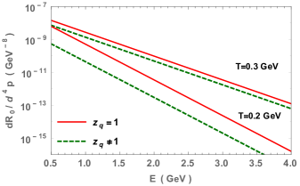
Figure 1: The equilibrium dilepton production rates with of $z_{q}^{2}$ as function of $T/T_{c}$ is shown along with its SB limit ($z_{q}\rightarrow 1$). The temperature dependence of the effective quark fugacity, $z_{q}$ is taken from Ref. chandra_quasi .

It is be noted that all above analysis were done in the rest frame of the medium, therefore in general frame with four-velocity $u^{\mu}$, these results become,

$$\frac{dR_{0}}{d^{4}p}^{\small{l^{+}l^{-}}} = \frac{z_{q}^{2}}{2}~{}\frac{M^{2}g^{2}\sigma(M^{2})}{(2\pi)^{5}}~{}e^{-u\cdot p/T},$$ (38)

$$\frac{dR_{1}}{d^{4}p}^{\small{l^{+}l^{-}}} = -\frac{8}{9}\frac{1}{T^{4}}\left(\frac{\hat{q}_{q}}{T^{3}}\right)^{-1}\left[\frac{u\cdot p}{4}+\frac{1}{3}~{}T^{2}\partial_{T}\,ln(z_{q})\right]$$

$$\times\frac{dR_{0}}{d^{4}p}^{\tiny{l^{+}l^{-}}}\left[p^{\mu}p^{\nu}\Delta u_{\mu\nu}\right],\,$$

where we have kept the term $\hat{q}_{q}/T^{3}$ for phenomenological reasons stated in the previous session.

We now proceed to study the QGP thermal dilepton spectra from heavy-ion collisions with non-equilibrium contributions.

IV Thermal dilepton yield from QGP during fireball evolution

To study dilepton yield from the QGP phase in heavy-ion collisions, we need to model expansion of the thermalised fireball. This can be done using relativistic hydrodynamics. In this qualitative analysis, we use the longitudinal boost invariant flow model of BjorkenBjorken:1982qr to describe the expanding system. In the Bjorken flow, with the parametrization $t=\tau$ cosh$\,\eta_{s}$ and $z=\tau$ sinh$\,\eta_{s}$; with the proper time $\tau=\sqrt{t^{2}-z^{2}}$ and space-time rapidity $\eta_{s}=\frac{1}{2}\,ln[\frac{t+z}{t-z}]$; the four velocity of the medium is written as $u^{\mu}=(\rm{cosh}\,\eta_{s},0,0,\rm{sinh}\,\eta_{s})$. Neglecting the effects of viscosity, now we can write the energy dissipation equation for the system asBjorken:1982qr

$$\frac{d\varepsilon}{d\tau}+\frac{\varepsilon+P}{\tau}=0.$$ (39)

Here $\varepsilon$ is the energy density and $P$ is the pressure of the system. Above equation need to be closed by providing equation of state (EoS). We use recent lattice QCD EoS cheng for this purpose. We take the transition temperature $T_{C}$, denoting the end of QGP phase, as $180$ MeV in this analysis. By providing the initial conditions i.e.; $\tau_{0}=0.5$ fm/c and $T(\tau_{0})=300$ MeV relevant for RHIC energies, we now solve the energy dissipation equation numerically to obtain the temperature profile $T(\tau)$.

Equipped with the temperature dependent thermal dilepton production rates, dilepton yield from the QGP can be obtained by integrating these rates over the space-time history of the fireball evolution,

$$\frac{dN}{d^{4}p}^{\small{l^{+}l^{-}}}=\int d^{4}x\,\frac{dR}{d^{4}p}^{\small{l^{+}l^{-}}}.$$ (40)

The four-volume element within Bjorken model is given by $d^{4}x=\pi R_{A}^{2}d\eta_{s}\tau d\tau$. Here $R_{A}=1.2A^{1/3}$ is the radius of the nucleus used for the collision and for $Au,~{}A=197$. We parametrise the four momentum of the dilepton as $p^{\alpha}$ = $(m_{T}coshy,p_{T}cos\phi_{p},p_{T}sin\phi_{p},m_{T}sinhy)$ with $m_{T}^{2}$ = $p_{T}^{2}+M^{2}$. The factors appearing in the rate expressions i.e.; Eq. (38) to be used in above integral are given as $u.p=m_{T}cosh(y-\eta_{s})$ and

$$p^{\alpha}p^{\beta}\Delta u_{\mu\nu} = -\frac{\,M^{2}}{3\tau}-\frac{m_{T}^{2}}{\tau}\,sinh^{2}(y-\eta_{s}).$$ (41)

Desired dilepton yields in terms of invariant mass $M$, transverse momentum $p_{T}$ and momentum rapidity $y$ are now given by

$$\frac{dN^{\tiny{l^{+}l^{-}}}}{dM^{2}d^{2}p_{T}dy} = \pi R_{A}^{2}\int_{\tau_{0}}^{\tau_{f}}d\tau~{}\tau\int_{-\infty}^{\infty}d\eta_{s}\,\frac{1}{2}\frac{dR}{d^{4}p}^{\tiny{l^{+}l^{-}}}$$ (42)

$$= \frac{dN_{0}^{\tiny{l^{+}l^{-}}}}{dM^{2}d^{2}p_{T}dy}+\frac{dN_{1}^{\tiny{l^{+}l^{-}}}}{dM^{2}d^{2}p_{T}dy}.$$

After performing the $\eta_{s}$ integration, the equilibrium and non-equilibrium contributions to the total dilepton yield are obtained as,

$$\frac{dN_{0}^{\tiny{l^{+}l^{-}}}}{dM^{2}d^{2}p_{T}dy} = \mathscr{R}\int_{\tau_{0}}^{\tau_{f}}\tau\,d\tau\,z_{q}^{2}\,2K_{0}(z_{m}),$$ (43)

$$\frac{dN_{1}^{\tiny{l^{+}l^{-}}}}{dM^{2}d^{2}p_{T}dy} = -\frac{8}{9}\mathscr{R}\,\int_{\tau_{0}}^{\tau_{f}}d\tau\,\frac{z_{q}^{2}}{T^{4}}\,\left(\frac{\hat{q}_{q}}{T^{3}}\right)^{-1}\mathscr{T}(T,p),$$

$${\rm with},\,\mathscr{T}(T,p) = K_{0}(z_{m})\,\bigg{\{}\frac{1}{3}T^{2}\partial_{T}\,ln(z_{q})\left(m_{T}^{2}-\frac{2}{3}M^{2}\right)\bigg{\}}$$

$$+K_{1}(z_{m})\,\bigg{\{}\frac{m_{T}^{3}}{8}-\frac{1}{6}M^{2}m_{T}\bigg{\}}$$

$$-K_{2}(z_{m})\,\bigg{\{}\frac{1}{3}T^{2}\partial_{T}\,ln(z_{q})\,m_{T}^{2}\bigg{\}}$$

$$-K_{3}(z_{m})\,\bigg{\{}\frac{m_{T}^{3}}{8}\bigg{\}},$$

$${\rm and},\,\,\,\mathscr{R} = \left[\frac{\pi R_{A}^{2}}{2^{2}}\frac{1}{(2\pi)^{5}}\frac{80\pi\alpha^{2}}{9}\right].$$

Here $K_{n}$ are the modified Bessel functions of the second kind and $z_{m}\equiv m_{T}/T$. Now we numerically integrate the above integrals with temperature profile obtained from hydrodynamical analysis to get the dilepton yields. All the results are presented for the midrapidity region of the dilepton i.e.; $y=0$.

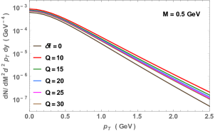
Figure 2: Dilepton yields with non-equilibrium effects for different $\hat{q}_{q}/T^{3}\equiv Q$ values for $M=0.5$ GeV. Equilibrium yield contribution is also plotted ($\delta f=0$).

The thermal dilepton yields as a function of transverse momentum of the dileptons for the invariant mass $M=0.5$ GeV are shown in Fig. 2. The non-equilibrium effects are included with various jet-quenching parameter $\hat{q}_{q}/T^{3}$ values. The equilibrium contribution alone is also plotted ($\delta f=0$) for comparison. It can be seen that the effect of non-equilibrium terms is to enhance the dilepton spectra throughout the $p_{T}$ regime. Also, as we increase the $\hat{q}_{q}/T^{3}$ value, yield decreases and approaches the equilibrium value. From Eqs.(38) & (41), it is clear that non-equilibrium contribution to dilepton rates is addictive, hence we see an increase in the yields with the inclusion of non-equilibrium terms.

Notably, with $\hat{q}_{q}/T^{3}=15$, we observe $\sim 38\%$ enhancement at $p_{T}=0.5$ GeV and $\sim 147\%$ at $p_{T}=2$ GeV. Since, $\hat{q}_{q}/T^{3}$ term appear in denominator of the yield expression, as seen in Eq. (43), increasing its value will result in the decrease of non-equilibrium contribution. For e.g.; for $\hat{q}_{q}/T^{3}=25$, enhancement is only about $\sim 23\%$ and $\sim 88\%$ for transverse momenta 0.5 GeV and 2 GeV respectively.

It is crucial to note that enhancement of the spectra is more significant at high $p_{T}$, indicating the strong non-equilibrium effects at that regime. In heavy-ion collisions, high $p_{T}$ particles are produced during the initial stages of the evolution. Since we expect the anisotropic effects also to be dominant at the initial stages of the evolution, its effect will be more effective at high $p_{T}$. The fact that enhancement is seen in low $p_{T}$ particles indicate that the non-equilibrium effects remain significant throughout the evolution of the system. We note that just like the overall effect of viscosities as seen in Ref.Chandra:2015rdz , present non-equilibrium effect also enhances the thermal dilepton spectra.

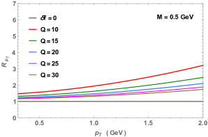
Figure 3: Strength of non-equilibrium corrections to equilibrium yield represented through ratio $R_{p_{T}}$ (Eq. (44)) for different jet quenching parameters.

Next, we study the strength of these non-equilibrium corrections to equilibrium distribution functions by looking into their contributions to dilepton spectra. We begin our analysis by constructing the following ratio

$$R_{p_{T}}=\frac{dN^{\tiny{l^{+}l^{-}}}}{dM^{2}d^{2}p_{T}dy}/\frac{dN_{0}^{\tiny{l^{+}l^{-}}}}{dM^{2}d^{2}p_{T}dy},$$ (44)

where numerator includes non-equilibrium contributions. We plot this ratio as a function of transverse momenta of the dileptons for different $\hat{q}_{q}/T^{3}$ values in Fig. 3.

Note that, for smaller value of transverse momentum, the non-equilibrium contribution is changing the equilibrium part by $\sim 50\%$ for $\hat{q}_{q}/T^{3}>10$. These non-equilibrium contributions tend to increase strongly as we move towards higher, $p_{T}$. The corrections start decreasing as we increase the $\hat{q}_{q}/T^{3}$ parameter as expected, since high values of $\hat{q}_{q}/T^{3}$ dilutes non-equilibrium corrections. For $\hat{q}_{q}/T^{3}=20(30)$, the contribution begins with $\sim 28(19)\%$ at $p_{T}=0.5$ GeV and reaches to $\sim 110(74)\%$ by $p_{T}=2$ GeV. Overall, we observe strong corrections to the yield by non-equilibrium effects.

It is to be emphasised that for low values of $\hat{q}_{q}/T^{3}$, significant corrections to spectra are seen. These strong corrections due to perturbative non-equilibrium effects are indicative of the fact that such $\hat{q}_{q}/T^{3}$ values are preferably ruled out within the present model. However to substantiate the claim thoroughly, one may need to perform a quantitative analysis including three-dimensional hydrodynamical flow, which is beyond the scope of this paper. Moreover, we recall that, in the present work, the corrections to spectra are calculated within one dimensional Bjorken flow, which is known to overestimate the particle spectra. So the corrections shown in this qualitative study act only as upper bounds. The precise nature of corrections to particle yields depends very much upon the geometry under consideration (here, simplified Bjorken), because of the involved space-time integration (which we perform numerically). How a different, more realistic three-dimensional geometry involving transverse flow will change the overall corrections, cannot be guessed. Although, it is expected that the effect of transverse flow is to decrease the particle yield, since the evolution time and therefor the limit of proper time integration, will be less in that case. However, the space part integration contribution is non-trivial and may change significantly under a different geometry.

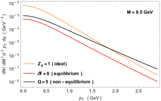
Figure 4: Strength of non-equilibrium terms via ratio $R_{p_{T}}$

Finally, let us analyze, how the non-equilibrium corrections and equilibrium values are modifying the ideal case i.e.; $z_{q}=1$. Yield corresponding to $ideal$ case can be obtained by considering Eq.(27) with $z_{q}=1$. The effect of $z_{q}^{2}$ term on the ideal spectra was analyzed by the authors in detail elsewhere Chandra:2015rdz and wont be repeated here. We recall that it’s effect was found to be suppressive and it can also be inferred from Fig. 1 of this manuscript. In Fig. 4, we plot the equilibrium and non-equilibrium dilepton yield for $M=0.5$ GeV with that for the ideal case. For non-equilibrium part, we have taken the jet quenching parameter value as $\hat{q}_{q}/T^{3}=5$ (This is typically the value that we obtain by averaging the predictions of all these approaches burke ; 55 ; 50 ; 51 ; 56 ; 42 ). For low transverse momenta, non-equilibrium enhancement of equilibrium spectra is marginal compared to the $ideal$ values. We observe that the non-equilibrium effects can overtake the $z_{q}$ suppressions of ideal spectra ($z_{q}=1$) at high $p_{T}$s. At at $p_{T}\sim 2$ GeV, we have near cancellation of these effects. However, thereafter non-equilibrium contribution will dominate other two. However, by increasing the jet quenching parameter, strength of the $z_{q}$ suppressions can be made dominate so that total spectra will become less than less than $ideal$ case.

It is to be emphasized that in the present, qualitative study, we have used one-dimensional Bjorken flow to model the system. It is well known that Bjorken results tend to over-estimate the particle production because system takes more time to cool down compared to realistic three-dimensional expansion with the transverse flow Bhatt:2011kx . However, such a quantitative study is not within the scope of present analysis and will be taken up for investigation the near future. It is encouraging that we are seeing very significant effects with one-dimensional flow, which, we believe, may guide us to have observable signatures on realistic three-dimensional calculations.

V Conclusions and outlook

In conclusion, thermal particle production is investigated in the presence of momentum anisotropy during the hydrodynamical expansion of the QGP in heavy-ion collisions. The effects of anisotropy are encoded in the non-equilibrium part of the quark/anti-quarks and gluon momentum distribution functions. We particularly, studied the dilepton production rate and compared our results against the isotropic/equilibrium case. The modifications induced by the anisotropy are found to be significant as far as the rate and dilepton yields are concerned. The strength of anisotropy, which in our case, is inversely proportional to the jet quenching parameter apart from other momentum dependent factors, have appreciable impact on the rate and yield. The whole analysis is based on an effective transport equation which is obtained by an ensemble averaging of the turbulent gluonic fields created due to the momentum anisotropy by inducing instability in $SU(3)$ Yang-Mills equations. We can perhaps treat the thermal particle production in the presence of the momentum anisotropy as the indicator of the impact of turbulent color-fields and anomalous transport processes during the expansion of QGP.

It would be interesting to include collisional processes and study the interplay of the them with anomalous ones by setting up and solving appropriate transport equation for the non-equilibrium distributions. We intend to employ them to study thermal particle production in heavy-ion collisions.

References

- (1) J. Adams et al. (STAR collaboration), Nucl. Phys. A 757, 102 (2005); K. Adcox e͡t al. (PHENIX Collaboration), Nucl. Phys. A 757 184 (2005); B. Back et al. (PHOBOS Collaboration), Nucl. Phys. A 757, 28 (2005); A. Arsence et al. (BRAHMS Collaboration), Nucl. Phys. A 757, 1 (2005).
- (2) K. Aamodt et al. (The Alice Collaboration), arXiv:1011.3914 [nucl-ex]; Phys. Rev. Lett. 105, 252301 (2010), Phys. Rev. Lett. 106, 032301 (2011).
- (3) L. Del Zanna et. al, Eur. Phys. J. C 73, 2524 (2013); V. Rolando et. al, Nuclear Physics A 931, 970-974 (2014). F. Becattini et. al, Eur. Phys. J. C 75, 406 (2015).
- (4) B. Schenke, S. Jeon, C. Gale, Phys. Rev. Lett. 106, 042301 (2011).
- (5) P. Bozek, Phys. Rev. C 85, 034901 (2012);
- (6) U. Heinz and R. Snellings, Ann. Rev. Nucl. Part.Sci. 63, 123 (2013).
- (7) C. Gale, S. Jeon, and B. Schenke, Int. J. Mod. Phys. A28, 1340011 (2013).
- (8) H. Song and U. W. Heinz, Phys .Rev. C 81, 024905 (2010).
- (9) H. Niemi, G. S. Denicol, P. Huovinen, E. Molnar, and D. H. Rischke, Phys. Rev. Lett. 106, 212302 (2011).
- (10) J. Randrup and S. Mrowczynski, Phys. Rev c 68, 034909 (2003).; P. Arnold, J. Lengaghan, and G. D. Moore, J. High Energy Phys. 08 (2003) 002; A. H. mueller, A. I. Shoshi, and S. M. H. Wong, Phys. Lett. B 632, 257 (2006).
- (11) S. Mrowczynski, B. Schenke, M. Strickland, Physics Reports (2017) ( http://dx.doi.org/10.1016/j.physrep.2017.03.003.)
- (12) M. Asakawa, S. A. Bass, B. Müller, Phys. Rev. Lett. 96, 252301 (2006); Prog. Theor. Phys. 116, 725 (2007).
- (13) V. Chandra and V. Ravishankar, Euro. Phys. J C 64, 63 (2009).
- (14) T. Abe and K. Niu, J. Phys. Soc. Jpn. 49, 717 (1980), ibid. 49, 725 (1980); S. Mrowczynski, Phys. Lett. B214, 587 (1988); ibid 314, 118 (1993); P. Romatschke and M. Strickland, Phys. Rev. D 68, 036004 (2003).
- (15) P. Arnold, J. Lengaghan, G. D. Moore, and L. G. Yaffe, Phys. Rev. Lett. 94, 072302 (2005).
- (16) J. Berges, K. Boguslavski, S. Schlichting, Phys. Rev. D 85, 076005 (2012), J. Berges, S. Scheffler, S. Schlichting, D. Sexty, Phys. Rev. D 85, 034507 (2012); Phys. Rev. D 86, 074006 (2012). Berges, S. Schlichting, Phys. Rev. D 87, 014026 (2013).
- (17) J. Berges, K. Boguslavski, S. Schlichting, R. Venugopalan, J. High Energy Phys. 05 (2014) 054, J. Berges, K. Boguslavski, S. Schlichting, R. Venugopalan, Phys. Rev. D 89, 074011 (2014); Phys. Rev. D 89, 114007 (2014), Phys. Rev. Lett. 114, 061601 (2015).
- (18) K. Fukushima, Phys. Rev. C 89, 024907 (2014).
- (19) K. Fukushima, F. Gelis, Nuclear Phys. A 874, 108 (2012).
- (20) A. Kurkela, G. D. Moore, arxiv:1209.4091[hep-lat].
- (21) A. Kurkela, G. D. Moore, Phys. Rev. D 86, 056008 (2012).
- (22) Erich S. Weibel, Phys. Rev. Lett. 2, 83 (1959).
- (23) T. H. Dupree, Phys. Fluids 9, 1773 (1966); ibid 11, 2680 (1968).
- (24) Vinod Chandra, S. K. Das, Phys. Rev. D 93, 094036 (2016), [arXiv:1506.07805 [nucl-th].]; S. K. Das, Vinod Chandra, Jane Alam, J. Phys. G 41 015102 (2013) [arXiv:1210.3905[nucl-th]].
- (25) S. K. Das, F. Scardina, S. Plumari, V. Greco, Phys. Lett. B 747, 260 (2015).
- (26) J. Alam, B. Sinha and S. Raha, Phys. Rept. 273 (1996) 243.
- (27) J. Alam, S. Sarkar, P. Roy, T. Hatsuda and B. Sinha, Annals Phys. 286 (2001) 159 [arXiv:hep-ph/9909267].
- (28) T. Peitzmann and M. H. Thoma, Phys. Rept. 364 (2002) 175 [arXiv:hep-ph/0111114].
- (29) H. Van Hees and R. Rapp, Nucl. Phys. A 806 (2008) 339 [arXiv:0711.3444 [hep-ph]].
- (30) L. D. McLerran, T. Toimela, Phys. Rev. D31 (1985) 545.
- (31) J. R. Bhatt, H. Mishra and V. Sreekanth, JHEP 1011 (2010) 106 doi:10.1007/JHEP11(2010)106 [arXiv:1011.1969 [hep-ph]].
- (32) J. R. Bhatt and V. Sreekanth, Int. J. Mod. Phys. E 19 (2010) 299 doi:10.1142/S0218301310014765 [arXiv:0901.1363 [hep-ph]].
- (33) J. Peralta-Ramos and M. S. Nakwacki, arXiv:1010.3672 [hep-ph].
- (34) J. R. Bhatt, H. Mishra and V. Sreekanth, Nucl. Phys. A 875 (2012) 181 [arXiv:1101.5597 [hep-ph]].
- (35) R. S. Bhalerao, A. Jaiswal, S. Pal and V. Sreekanth, Phys. Rev. C 88 (2013) 044911 [arXiv:1305.4146 [nucl-th]].
- (36) V. Chandra and V. Sreekanth, Phys. Rev. D 92 (2015) 9, 094027 [arXiv:1511.01208 [nucl-th]].
- (37) V. Chandra and V. Ravishankar, Euro. Phys. J C 59, 705 (2009)
- (38) V. Chandra, V. Ravishankar, Phys. Rev. D 84, 074013 (2011).
- (39) M. Cheng et. al, Phys. Rev. D 77, 014511 (2008).
- (40) S. Borsanyi et. al, JHEP 1009,073 (2010); JHEP 11, 077 (2010); Y. Aoki et al., JHEP 0601, 089 (2006); JHEP 0906, 088 (2009).
- (41) Vinod Chandra, Phys. Rev. D 86, 114008 (2012), Phys. Rev. D 84, 094025 (2011).
- (42) Sukanya Mitra, Vinod Chandra, Phys. Rev. D 94, 034025 arXiv:1606.08556 [nucl-th].
- (43) A. Peshier et. al, Phys. Lett. B 337, 235 (1994), Phys. Rev. D 54, 2399 (1996).
- (44) A. Peshier, B. Kampfer, G. Soff, Phys.Rev. C 61, 045203 (2000); Phys.Rev. D 66, 094003 (2002).
- (45) M. DÉlia, A. Di Giacomo, E. Meggiolaro, Phys. Lett. B 408, 315 (1997); Phys. Rev. D 67, 114504 (2003); P. Castorina, M. Mannarelli, Phys. Rev. C 75, 054901 (2007); Phys. Lett. B 664, 336 (2007);
- (46) A. Dumitru and R. D. Pisarski, Phys. Lett. B 525, 95 (2002); K. Fukushima, Phys. Lett. B 591, 277 (2004); S. K. Ghosh et al., Phys. Rev. D 73, 114007 (2006); H. Abuki, K. Fukushima, Phys. Lett. B 676, 57 (2006); H. M. Tsai, B M ̵̈ller, J. Phys. G 36, 075101 (2009); M. Ruggieri et. al, Phys. Rev. D 86, 054007 (2012).
- (47) P. Alba, W. Alberico, M. Bluhm, V. Greco, C. Ratti, M. Ruggieri, Nucl. Phys. A 934 ,41-51 (2015).
- (48) S. Jeon, Phys. Rev. D 52, 3591 (1995), S. Jeon, L.G. Yaffe, Phys. Rev. D 53 5799(1996).
- (49) M. Bluhm, B. Kampfer, K. Redlich, Nucl. Phys. A 830, 737c-740c (2009).
- (50) K. Dusling, and T, Schäfer, Phys. Rev. C 77, 034905 (2008); K. Dusling, and D. Teaney, Phys. Rev. C 85, 044909 (2012).
- (51) M. Bluhm, B. Kampfer, R. Schulze, D. Seipt, U. Heinz, Phys. Rev. C 76, 034901 (2007).
- (52) P. Chakraborty, J. I. Kapusta, Phys. Rev. C 83, 014906 (2011).
- (53) J. D. Bjorken, Phys. Rev. D 27 (1983) 140.
- (54) U. W. Heinz, Phys. Rev. Letts. 51,351 (1983).
- (55) U. W. Heinz, Annals Phys. 161, 48 (1985).
- (56) U. W. Heinz, Annals Phys. 168, 148 (1986).
- (57) A. Majumdar, B. Muller, and X.-N. Wang, Phys. Rev. Lett. 99, 192301 (2007).
- (58) K. M. Burke et al , arXiv:1312.5003v2[nucl-th].
- (59) M. Asakawa, S. A. Bass, B. Müller, Nucl. Phys. A854, 76-80 (2011).
- (60) A. Buzzatti and M. Gyulassy, Phys. Rev. Lett. 108, 022301 (2012.
- (61) X. -F. Chen, T. Hirano, E. Wang, X. -N. Wang and H. Zhang, Phys. Rev. C 84, 034902 (2011) [arXiv:1102.5614 [nucl-th]].
- (62) A. Majumder and C. Shen, Phys. Rev. Lett. 109, 202301 (2012) [arXiv:1103.0809 [hep-ph]].
- (63) B. Schenke, C. Gale and S. Jeon, Phys. Rev. C 80, 054913 (2009) [arXiv:0909.2037 [hep-ph]].
- (64) G. Y. Qin, J. Ruppert, C. Gale, S. Jeon, G. D. Moore and M. G. Mustafa, Phys. Rev. Lett. 100, 072301 (2008) [arXiv:0710.0605 [hep-ph]].
- (65) S. Mrowczynski, Phys. Lett. B 314, 118?121 (1993). Phys. Rev. C 49, 2191?2197 (1994). Phys. Lett. B 393, 26?30 (1997).
- (66) P. Arnold, J. Lenghan, G. D. Moore, and L. G. Yaffe, Phys. Rev. Lett. 94, 072302 (2005).
- (67) A. Rebhan, P. Romatschke, and M. Strickland, Phys. Rev. Lett., 94, 102303 (2005).
- (68) P. Romatschke and R. venugopalan, Physical Review Lett. 96, 062302 (2006).
- (69) P. Romatschke and M. Strickland, Phys. Rev. D 68, 036004 (2003), P. Romatschke and M. Strickland, Phys. Rev. D 70, 116006 (2004).
- (70) M. E. Carrington, K. Deja and S. Mrowczynski, Phys. Rev. C 90 (2014) no.3, 034913.
- (71) M. Yousuf Jamal, S. Mitra and Vinod Chandra, arXiv:arXiv:1701.06162v1 [nucl-th] (To appear in Phys. Rev. D (2017)).
- (72) Romatschke and M. Strickland, Phys. Rev. D 71, no. 12, 125008 ( 2005).
- (73) P. Romatschke, Phys. Rev. C 75, no. 1, 014901 (2007).
- (74) P. Roy and A. K. Dutt-Mazumder, Phys. Rev. C 83, no. 4, 044904 (2011).
- (75) J. Ruppert and B. Muller, Phys. Lett. B 618, 123?130 ( 2005), P. Chakraborty, M. G. Mustafa, and M. H. Thoma, Phys. Rev. D 74, no. 9, 094002 (2006).
- (76) M. Mandal and P. Roy, Advances in High Energy Physics 2013 (2013), 371908.
- (77) R. Vogt, Ultrarelativistic Heavy-Ion Collisions, Elsevier, (2007).