Beyond the locally tree-like approximation for percolation on real networks

Abstract

Theoretical attempts proposed so far to describe ordinary percolation processes on real-world networks rely on the locally tree-like ansatz. Such an approximation, however, holds only to a limited extent, as real graphs are often characterized by high frequencies of short loops. We present here a theoretical framework able to overcome such a limitation for the case of site percolation. Our method is based on a message passing algorithm that discounts redundant paths along triangles in the graph. We systematically test the approach on $98$ real-world graphs and on synthetic networks. We find excellent accuracy in the prediction of the whole percolation diagram, with significant improvement with respect to the prediction obtained under the locally tree-like approximation. Residual discrepancies between theory and simulations do not depend on clustering and can be attributed to the presence of loops longer than three edges. We present also a method to account for clustering in bond percolation, but the improvement with respect to the method based on the tree-like approximation is much less apparent.

Percolation processes are often used to study resilience properties of real networks Albert et al. (2000); Cohen et al. (2000); Callaway et al. (2000), and play a fundamental role in the understanding of spreading phenomena in real systems Pastor-Satorras and Vespignani (2001); Newman (2002). Percolation has been intensely studied in a multitude of network models Dorogovtsev et al. (2008); Dorogovtsev (2010); Newman (2010), including sparse tree-like graphs  Cohen et al. (2000); Callaway et al. (2000); Cohen et al. (2002), as well as generative models for random networks with triangles, cliques or arbitrary subgraphs Serrano and Boguñá (2006a, b); Gleeson (2009); Newman (2009); Miller (2009); Gleeson et al. (2010). These studies shed light on fundamental physical mechanisms of percolation processes on complex network topologies, but their importance in the analysis of percolation on real-world graphs is limited, as the topology of individual real networks often markedly differs from the one of random network ensembles. Recent works have attempted to overcome such a serious limitation. Karrer et al. formulated a novel method which takes as input the detailed topological structure of a given network to predict the value of the percolation strength (and other macroscopic observables) as a function of the bond occupation probability Karrer et al. (2014). In particular, they demonstrated that the bond percolation threshold of a given network is bounded from below by the leading eigenvalue of its non-backtracking matrix Hashimoto (1989). An approach based on the same rationale was also used by Hamilton and Pryadko to study site percolation in isolated networks Hamilton and Pryadko (2014), and by Radicchi in the analysis of bond and site percolation models in interdependent networks Radicchi (2015a). These methods still suffer from a fundamental limitation: they are based on the locally tree-like approximation Dorogovtsev et al. (2008); Dorogovtsev (2010); Newman (2010), and as such they are potentially not reliable for networks with nonnegligible density of triangles, or short loops in general Radicchi (2015b); Faqeeh et al. (2015).

In this paper, we make a step forward, by generalizing the approach developed in Hamilton and Pryadko (2014); Karrer et al. (2014) to clustered networks. Through a systematic analysis of about one hundred real-world networks as well as clustered synthetic ones, we demonstrate that our framework provides excellent prediction of the whole phase diagram for the site percolation model. Furthermore, we present an approach improving also the prediction of the bond percolation phase diagram (though in a less satisfactory way) and understand the origin of the differences between the two cases.

We start our analysis from the site percolation model. We assume that the structure of a network with $N$ nodes and $E$ edges is given by a one-zero adjacency matrix $A$ (i.e., the generic element $A_{i,j}=1$ if vertices $i$ and $j$ are connected, whereas $A_{i,j}=0$ otherwise). We further assume that the network is composed of a single connected component. In the ordinary site percolation model, each node is active or occupied with probability $p$. Two active nodes belong to the same cluster if there exists at least a path, passing only through active nodes, that connects them. For $p=0$, no nodes are active so that there are no clusters. For $p=1$, all nodes are active and belong to a single cluster of size $N$. As $p$ varies, the network undergoes a structural phase transition, at the percolation threshold $p_{c}$, corresponding to the appearance of an extensive cluster. The transition can be monitored through the so-called percolation strength $S_{\infty}$, defined as the relative size of the largest cluster with respect to the size of the network. For $p=0$, $S_{\infty}=0$; for $p=1$, $S_{\infty}=1$. The goal of the following approach is to estimate the expected value of $S_{\infty}$ over an infinite number of realizations of the percolation model for any given value of $p$. The probability $s_{i}$ that node $i$ belongs to the largest cluster can be described by the equation

$$s_{i}=p[1-\prod_{j\in\mathcal{N}_{i}}(1-t_{i\to j})]\;,$$ (1)

where $\mathcal{N}_{i}$ is the set of neighbors of node $i$ and $t_{i\to j}$ quantifies the probability that following the edge $(i,j)$, in the direction $i\to j$, we find a node belonging to the largest cluster. The quantity $t_{i\to j}$ can be interpreted as a “message” passed from node $j$ to vertex $i$ about belonging to the largest cluster. Eq. (1) essentially states that the probability that node $i$ is part of the largest cluster equals the product of the probabilities that (i) node $i$ is active and (ii) at least one of its neighbors is in the largest cluster. For consistency, the probability $t_{i\to j}$ is described by the equation

$$t_{i\to j}=p[1-\prod_{k\in\mathcal{Q}_{i\to j}}(1-t_{j\to k})]\;.$$ (2)

The explanation of this equation is similar to the previous one. The only difference here is that the product does not run necessarily over all the neighbors of node $j$, but only on the elements of the set $\mathcal{Q}_{i\to j}$. We note that, while Eq. (2) is in principle defined for every pair of node indices $i\to j$, only pairs of nodes connected by an edge play a role in Eq. (1). We have therefore $2E$ equations of the type (2) that can be solved by iteration. The solutions of these equations are then plugged into the set of $N$ Eqs. (1) to determine the value of every $s_{i}$. Finally, the percolation strength is computed as

$$S_{\infty}=\frac{1}{N}\sum_{i}s_{i}\;.$$ (3)

Since the entire operation can be repeated for any value of the occupation probability $p$, Eqs. (1),  (2) and (3) allow to draw the entire phase diagram for a given network. A linear expansion of the system of Eqs. (2) can be used to obtain an eigenvalue/eigenvector equation of the type $\vec{t}=p\,G\,\vec{t}$, where $\vec{t}$ is a vector with $2E$ components, and $G$ is a $2E\times 2E$ one-zero matrix. A non trivial solution exists only if $1/p$ is an eigenvalue of the operator $G$. Thus the inverse of the largest eigenvalue of $G$ (which is real according to the Perron-Frobenius theorem) is the percolation threshold $p_{c}$ of the network.

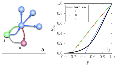
Figure 1: (a) Illustration of the different ways of defining $\mathcal{Q}_{i\to j}$ in Eq. (2). The $A$-based approximation is obtained by setting $\mathcal{Q}_{i\to j}=\mathcal{N}_{j}$, so all edges departing from $j$ are included in the equation. If backtracking walks are excluded, that is $\mathcal{Q}_{i\to j}=\mathcal{N}_{j}\setminus\{i\}$, the message passing equation will not include the green edge. we refer to this approximation as the $M$-based approximation. If $\mathcal{Q}_{i\to j}=\mathcal{N}_{j}\setminus[\{i\}\cup(\mathcal{N}_{j}\cap\mathcal{N}_{i})]$ so one can only move away from node $i$, also walking to node $k$ is avoided and the only terms appearing in the equation are given by those corresponding to the blue arrows. This corresponds to the $W$-based approximation. (b) Phase diagram for the site percolation model applied to co-authorship graph among network scientists Newman (2006). The black line denotes the results of numerical simulations of the model. The other curves represent results obtained through the numerical solution of Eqs. (1), (2) and (3) with different definitions of $\mathcal{Q}_{i\to j}$.

The form of $G$ depends on the definition of the set $\mathcal{Q}_{i\to j}$ in Eq. (2), which is crucial for the effectiveness of the entire approach. We illustrate here three different, and increasingly accurate, approximations (see Fig. 1a). In the first approximation, we set $\mathcal{Q}_{i\to j}=\mathcal{N}_{j}$. Such a choice makes Eq. (2) identical to Eq. (1), so that $t_{i\to j}=s_{j}$. The generic element of the matrix $G$ is $G_{i\to j,\ell\to k}=\delta_{j,\ell}$, with $\delta_{x,y}$ the Kronecker symbol. This matrix has the same eigenvalues of the adjacency matrix Karrer et al. (2014). Hence the percolation threshold under this approximation is given by the inverse of the leading eigenvalue of the adjacency matrix Bollobás et al. (2010). We refer to it as the adjacency-matrix-based or, in short, $A$-based approximation. In this approximation, the variable $t_{j\to i}$ is on the r.h.s. of Eq. (2), so that $t_{i\to j}$ grows as $t_{j\to i}$ increases. In turn, the value of $t_{j\to i}$ is also increased by the growth of $t_{i\to j}$. The possibility for a message to pass back and forth on the same edge causes an “echo chamber” effect in the equations that leads to an overestimation of the correct values of the variables $t$ and hence of the percolation strength. To suppress this effect, a more precise approximation prescribes $\mathcal{Q}_{i\to j}=\mathcal{N}_{j}\setminus\{i\}$. The motivation of this choice is simple: the exclusion of vertex $i$ from the product on the r.h.s. of Eq. (2) does not allow for backtracking messages, and the variable $t_{j\to i}$ does not appear anymore on the r.h.s. of Eq. (2). Under this approximation, $G$ coincides with $M$, the non-backtracking matrix of the graph Karrer et al. (2014), whose generic element is

$$M_{i\to j,\ell\to k}=\delta_{j,\ell}(1-\delta_{i,k})\;.$$ (4)

The percolation threshold is estimated as the inverse of the principal eigenvalue of the non-backtracking matrix of the graph Karrer et al. (2014); Radicchi (2015a). The $M$-based approximation is exact in networks with locally tree-like structure. However, if loops are present in the network, echo chamber effects still persist. This undesirable effect can be once more discounted by excluding redundant paths caused by triangles, that is using the following approximation

$$\mathcal{Q}_{i\to j}=\mathcal{N}_{j}\setminus[\{i\}\cup(\mathcal{N}_{j}\cap\mathcal{N}_{i})]\;.$$ (5)

The rationale behind Eq. (5) is again intuitive. If we are looking at the network from vertex $i$, we should disregard the path $i\to j\to k$ if we already considered the edge $i\to k$, otherwise vertex $i$ would receive twice the same message from node $k$. The importance of this correction is apparent in Fig. 1b, where the results of simulations for the site percolation model [see Supplemental Material (SM) for details] are compared with the numerical solutions of Eqs. (1), (2) and (3) adopting the three different definitions of $\mathcal{Q}_{i\to j}$ illustrated above. The network analyzed in Fig. 1b is a graph of scientific co-authorships characterized by a very high value of the clustering coefficient ($C=0.7412$) Newman (2006). As in the cases of the first two approximations, also the last, new approximation allows for the computation of the percolation threshold through the linearization of Eqs. (2). The critical value of the occupation probability is given by the inverse of the leading eigenvalue of the matrix $G=W$, defined as

$$W_{i\to j,\ell\to k}=\delta_{j,\ell}\,(1-\delta_{i,k})(1-A_{i,k})\;.$$ (6)

The definition of the matrix $W$ is very similar to the one of the non-backtracking matrix appearing in Eq. (4). The only difference is the additional term $(1-A_{i,k})$, that excludes connections among edges that are part of a triangle. In the matrix $W$, the directed edges $i\to j$ and $\ell\to k$ are connected only if $j=\ell$, and node $k$ is at distance two from vertex $i$. Mathematical arguments analogous to those presented by Karrer et al. Karrer et al. (2014) (see SM) show that the percolation threshold predicted using the $W$-based approximation is always larger than or equal to the one predicted using the $M$-based method (with the equality sign valid when no triangles are present), and always smaller than or equal to the true percolation threshold. Both these inequalities are validated in all numerical experiments on both real and synthetic networks. For the network of Fig. 1b, the $A$-based approximation predicts $p_{c}^{(A)}=0.0964$; the approximation based on the $M$ matrix gives $p_{c}^{(M)}=0.1148$; the approximation based on $W$ provides instead $p_{c}^{(W)}=0.4436$. Those predictions compared to the best estimate $p_{c}=0.6300$ from numerical simulations have associated relative errors respectively equal to $r^{(A)}=0.8470$, $r^{(M)}=0.8178$ and $r^{(W)}=0.2959$. These correspond to an improvement of roughly $3\%$ from the $A$-based to the $M$-based approximation, and more than $50\%$ from the $M$-based to the $W$-based approximation. The situation is qualitatively and quantitatively similar in all other real networks we consider in this study (see SM). We can conclude that the inverse of the largest eigenvalue of the matrix $W$ represents a tighter lower-bound of the true site percolation threshold than the analogous quantity computed using the $M$ matrix.

The $W$-based approximation is able to reproduce with impressive accuracy the whole percolation diagram of almost all the $98$ real networks we analyzed Radicchi (2015a). The only exceptions are spatially embedded networks and a few others, where the $W$-based approximation greatly outperforms the other approximations but still differs significantly from the numerical simulations. The results of our analysis are summarized in Fig. 2a, where relative errors in the estimates of the percolation threshold are plotted against the average clustering coefficients of the networks. We quantify the performance of the various approximations also in terms of the global error measure Melnik et al. (2011) $\int_{0}^{1}dp|S_{\infty}(p)-S_{\infty}^{(\alpha)}(p)|$, with $\alpha=A,M$ or $W$ (Fig. 2b). We remark that the discrepancy between the $W$-based approximation and simulations is essentially independent of the clustering coefficient $C$. This happens because the $W$-based approximation becomes exact in the infinite size limit for site percolation on networks containing only short loops of length three (see SM), such as two important classes of random network models with large clustering Gleeson (2009); Newman (2009); Miller (2009); Gleeson et al. (2010). The residual discrepancies in Fig. 2 depend only on the presence of longer loops, which do not contribute to the value of $C$. In the SM we also show that the $W$-based approximation can be in principle further improved to account for loops of length longer than three, but that a systematic approach becomes practically unfeasible already for loops of length four.

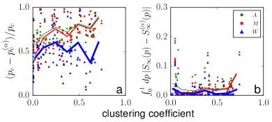
Figure 2: (a) Relative error associated to the estimation of the site percolation threshold for $98$ real networks. For the $\alpha$-based approximation, the relative error is measured as $(p_{c}-p_{c}^{(\alpha)})/p_{c}$, with $p_{c}^{(\alpha)}$ best estimate of the percolation threshold for the $\alpha$-based approximation [$\alpha=A,M$ or $W$], and $p_{c}$ value of the occupation probability corresponding to the peak of the susceptibility. The relative error is plotted against the average clustering coefficient of the network. Different colors and symbols correspond to different orders of the approximation. Full lines indicate average values of the relative error for networks with similar values of clustering coefficient. They are generated according to the following procedure. We divide the range of possible values of $C$ in seven equally spaced bins. We then estimate the average value of the error in each bin, and the average value of the cluster coefficient within each bin. The lines are obtained connecting these points. (b) Same as in panel a, but for the global error measure $\int_{0}^{1}dp|S_{\infty}(p)-S_{\infty}^{(\alpha)}(p)|$.

Next, we consider ordinary bond percolation on a given network. In this model, every edge is present or active with probability $p$. Clusters are formed by nodes connected by at least one path composed of active edges. The order parameter used to monitor the percolation transition, from the disconnected configuration at $p=0$ to the globally connected configuration for $p=1$, is still given by the relative size of the largest connected cluster, namely $B_{\infty}$. The message passing equations valid for the approximations based on the adjacency and on the non-backtracking matrices are identical to those already written for the site percolation model, with the only difference of a factor $p$ Radicchi and Castellano (2015). The order parameters are related by $B_{\infty}=p^{-1}\,S_{\infty}$, and the percolation thresholds predicted by the equations are identical in the two models Hamilton and Pryadko (2014); Karrer et al. (2014); Radicchi and Castellano (2015). Writing an improved approximation able to fully take into account triangles, such as the $W$-based approximation for site percolation, is in this case impossible (see SM). However, one can still write a similar approach which improves with respect to the two old methods. In the bond percolation model, a triangle is effectively present only if all its edges are simultaneously active, leading to the following self-consistent equations

$$b_{i}=1-\prod_{j\in\mathcal{N}_{i}}(1-p\,c_{i\to j})\;,$$ (7)

and

$$\begin{array}[]{l}c_{i\to j}=1-\prod_{k\in\mathcal{N}_{j}\setminus[\{i\}\cup(\mathcal{N}_{j}\cap\mathcal{N}_{i})]}(1-pc_{j\to k})\\ \prod_{k\in\mathcal{N}_{j}\cap\mathcal{N}_{i}}[1-pc_{j\to k}(1-p+pc_{i\to k})]\end{array}\;.$$ (8)

Here, $b_{i}$ and $c_{i\to j}$ have, in the bond percolation model, the same meaning that $s_{i}$ and $t_{i\to j}$ have in site percolation. The second equation explicitly imposes coherence of messages within triangles. The message from node $k$ can in fact arrive to node $i$ in two ways. (i) Along the path $k\to j\to i$ if the edge $(i,k)$ is not active but the edge $(i,j)$ is active. This possibility happens with probability $pc_{j\to k}(1-p)$. (ii) Simultaneously along the paths $k\to j\to i$ and $k\to i$ if both edges $(i,k)$ and $(i,j)$ are active. The latter possibility happens with probability $p^{2}c_{j\to k}c_{i\to k}$. In the absence of triangles, that means $\mathcal{N}_{j}\cap\mathcal{N}_{i}=\emptyset$ for all edges $(i,j)$, we recover the $M$-based approximation. In the presence of triangles instead, the additional correction term reduces the estimated values of the variables $c$. The system of Eqs. (8) can be solved by iteration. Its solutions can be then plugged into Eqs. (7), and the values of the variables $b_{i}$ can finally be used to compute the bond percolation strength as $B_{\infty}=N^{-1}\sum_{i}b_{i}$.

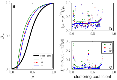
Figure 3: (a) Phase diagram for the bond percolation model applied to co-authorship graph among network scientists Newman (2006). The black line denotes the results of numerical simulations of the model. The other curves represent results obtained through the numerical solution of the equations using different approximations. (b) Relative error of the various approximations in the estimation of the bond percolation threshold. The figure represents the analogue of Fig. 2a for bond percolation. (c) Same as Fig. 2b but for bond percolation.

In Fig. 3a, we compare the performance of the approximations in reproducing the results of numerical simulations in the same network analyzed in Fig. 1b. The improvement in the prediction of the percolation strength from the adjacency matrix-based up to the $W$-based approximation is not as significant as the one we found for site percolation. The same qualitative observation can be made for the other real networks we analyzed (see SM). The linearization of the system of Eqs. (8) leads to the following vectorial equation for the determination of the percolation threshold

$$\vec{c}=p_{c}\,W\vec{c}+p_{c}(1-p_{c})(M-W)\vec{c}\;.$$ (9)

The solution of this equation can be efficiently obtained by means of a power-iteration algorithm combined with a binary search. As already done for site percolation, we systematically test the performance of the various approximations in $98$ real networks in Figs. 3b and 3c. In general, accounting in this way for triangles improves only slightly the accuracy of predictions with respect to the $M$-based approximation.

In summary, our novel approximation goes, in a relatively straightforward manner, beyond the locally tree-like ansatz. The analysis carried out on real and synthetic networks allows to conclude that the $W$-based approximation greatly outperforms the $M$-based approximation for the site percolation process, leading in almost all cases to an impressive agreement with numerical results. For bond percolation instead the improvement is less satisfactory and calls for further work. Systematic approximations to account for loops longer than three face severe intrinsic difficulties (see SM). It would be interesting to explore differences between the $M$-based and the $W$-based approximations in the context of ordinary percolation processes in interdependent networks Radicchi (2015a) as well in optimal percolation problems in isolated ones Morone and Makse (2015). As a final remark, we stress that the improvement in the prediction of the percolation threshold comes at a price. Whereas the computational complexity of the algorithm is the same in both $M$- and $W$-based approximations, the determination of $p_{c}$ in the $W$-based approximation requires to deal with a larger matrix. The Ihara-Bass determinant formula is able to reduce the computation of the largest eigenvalue of the $2E\times 2E$ non-backtracking matrix $M$ to the largest eigenvalue of a $2N\times 2N$ matrix Bass (1992). The quest for a similar formula for the matrix $W$ is an interesting challenge for future research.

This work is partially supported by the National Science Foundation (Grant CMMI-1552487).

References

- Albert et al. (2000) R. Albert, H. Jeong, and A.-L. Barabási, Nature 406, 378 (2000).
- Cohen et al. (2000) R. Cohen, K. Erez, D. Ben-Avraham, and S. Havlin, Phys. Rev. Lett. 85, 4626 (2000).
- Callaway et al. (2000) D. S. Callaway, M. E. Newman, S. H. Strogatz, and D. J. Watts, Phys. Rev. Lett. 85, 5468 (2000).
- Pastor-Satorras and Vespignani (2001) R. Pastor-Satorras and A. Vespignani, Phys. Rev. Lett. 86, 3200 (2001).
- Newman (2002) M. E. Newman, Phys. Rev. E 66, 016128 (2002).
- Dorogovtsev et al. (2008) S. N. Dorogovtsev, A. V. Goltsev, and J. F. Mendes, Rev. Mod. Phys. 80, 1275 (2008).
- Dorogovtsev (2010) S. N. Dorogovtsev, Lectures on complex networks, vol. 24 (Oxford University Press Oxford, 2010).
- Newman (2010) M. Newman, Networks: an introduction (Oxford University Press, 2010).
- Cohen et al. (2002) R. Cohen, D. Ben-Avraham, and S. Havlin, Phys. Rev. E 66, 036113 (2002).
- Serrano and Boguñá (2006a) M. A. Serrano and M. Boguñá, Phys. Rev. Lett. 97, 088701 (2006a).
- Serrano and Boguñá (2006b) M. A. Serrano and M. Boguñá, Phys. Rev. E 74, 056115 (2006b).
- Gleeson (2009) J. P. Gleeson, Phys. Rev. E 80, 036107 (2009).
- Newman (2009) M. E. Newman, Phys. Rev. Lett. 103, 058701 (2009).
- Miller (2009) J. C. Miller, Phys. Rev. E 80, 020901 (2009).
- Gleeson et al. (2010) J. P. Gleeson, S. Melnik, and A. Hackett, Phys. Rev. E 81, 066114 (2010).
- Karrer et al. (2014) B. Karrer, M. E. J. Newman, and L. Zdeborová, Phys. Rev. Lett. 113, 208702 (2014).
- Hashimoto (1989) K.-i. Hashimoto, Automorphic forms and geometry of arithmetic varieties. pp. 211–280 (1989).
- Hamilton and Pryadko (2014) K. E. Hamilton and L. P. Pryadko, Phys. Rev. Lett. 113, 208701 (2014).
- Radicchi (2015a) F. Radicchi, Nature Phys. 11, 597 (2015a).
- Radicchi (2015b) F. Radicchi, Phys. Rev. E 91, 010801 (2015b).
- Faqeeh et al. (2015) A. Faqeeh, S. Melnik, and J. P. Gleeson, Phys. Rev. E 91, 052807 (2015).
- Newman (2006) M. E. Newman, Phys. Rev. E 74, 036104 (2006).
- Bollobás et al. (2010) B. Bollobás, C. Borgs, J. Chayes, O. Riordan, et al., Ann. Probab. 38, 150 (2010).
- Melnik et al. (2011) S. Melnik, A. Hackett, M. A. Porter, P. J. Mucha, and J. P. Gleeson, Phys. Rev. E 83, 036112 (2011).
- Radicchi and Castellano (2015) F. Radicchi and C. Castellano, Nat. Commun. 6, 10196 (2015).
- Morone and Makse (2015) F. Morone and H. A. Makse, Nature 524, 65 (2015).
- Bass (1992) H. Bass, Int. J. Math. 3, 717 (1992).