Car Type Recognition with Deep Neural Networks

Abstract

In this paper we study automatic recognition of cars of four types: Bus, Truck, Van and Small car. For this problem we consider two data driven frameworks: a deep neural network and a support vector machine using SIFT features. The accuracy of the methods is validated with a database of over 6500 images, and the resulting prediction accuracy is over 97 %. This clearly exceeds the accuracies of earlier studies that use manually engineered feature extraction pipelines.

I Introduction

Traffic counting is a central tool for traffic planning and analysis for intelligent traffic. In many cases the desire is to increase the level of details by additional categorization of vehicle types. This allows a more fine-grained analysis and more accurate profiling of users of the transportation infrastructure, which is necessary for assessing the effects of possible modifications in the traffic system.

There are several production-level techniques for recognition of vehicle types, including inductive ground loops (see, e.g., MAVE-L product line of AVE GmbH) and laser scanners (see, e.g., traffic counters from SICK GmbH). However, all these technologies require laborious installation and significant amount of costly hardware. In this paper we study the use of low cost cameras for car type classification. The benefits are obvious: Cameras are ubiquitous and cost-efficient tools for monitoring, and they often have also other surveillance uses simultaneously. However, the reliability of camera based technologies may be vulnerable to environmental factors, such as poor illumination, dirt or change of viewing angle, and the developed system should therefore be robust to such changes. A typical scenario uses camera based recognition for surveillance, categorizing the entering vehicles at the gate to an access controlled facility. In this case, the input to the algorithm would typically consist of frontal view pictures, such as those shown in Figure 1.

Earlier research related to the topic is divided into two main areas: car make recognition [1, 2] and car type recognition that has received a lot of attention during the recent years, [3, 4, 5]. From customer (traffic operator) viewpoint, the car type is typically more interesting than the car make, which is also our motivation to study this problem.

Kafai et al. [3] propose to use a Bayesian network for the vehicle type classification, with features extracted from images of the rear of the car. The resulting feature vector consists of a collection of geometric parameters of the vehicle; including simple features such as the vehicle width and height and more complicated features, such as the distance from the license plate to the tail lights. Subsequently, the most significant features from the pool are fed to a Bayesian network for classification. The authors report 10-fold cross-validated classification accuracy of 95.7% for a database of 177 vehicles from four categories.

Zhang et al. [4] propose a framework, where the reconstruction error of a vector quantization representation is used for car type classification. More specifically, a tight bounding box of the car is first extracted, and a codebook for each class is learned from the training data. The reconstruction error is used as a basis for a measure for the class confidence, and falsely detected object candidates are rejected by thresholding the classification error with a manually set limit. The authors report an accuracy of 92 % and over 95 % when the rejection heuristic is used. The database consists of over 2800 images.

In [5], the authors use a neural network for car type classification. The input to the network consists of a collection of image based features, such as width, height, perimeter and fractal dimension. The actual classification is done in two stages using two neural networks, and the authors report 69 % accuracy on a database with 100 vehicles.

All the above works rely on a more or less elaborate preprocessing step; at least an accurate vehicle detection and alignment resulting in a tight bounding box is required. In our work, we wish to avoid all preprocessing steps, as they may be computationally expensive and—more importantly—fragile to errors that may collapse the subsequent classification completely. Moreover, we will be considering an application, where high accuracy is required in various environmental conditions. In particular, poor illumination, dirt and snow are typically difficult for preprocessing steps, including detection and localization.

 

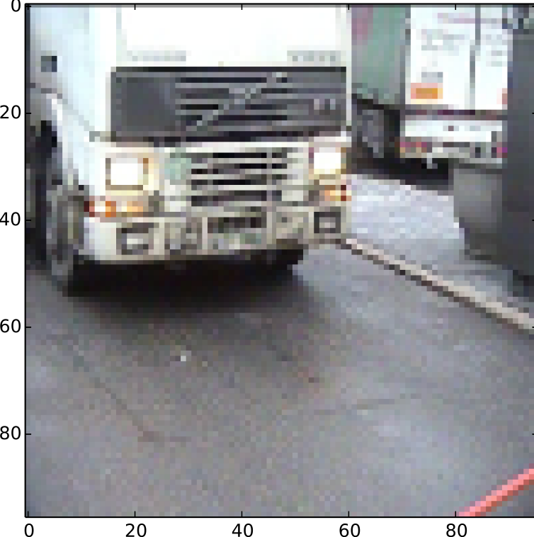
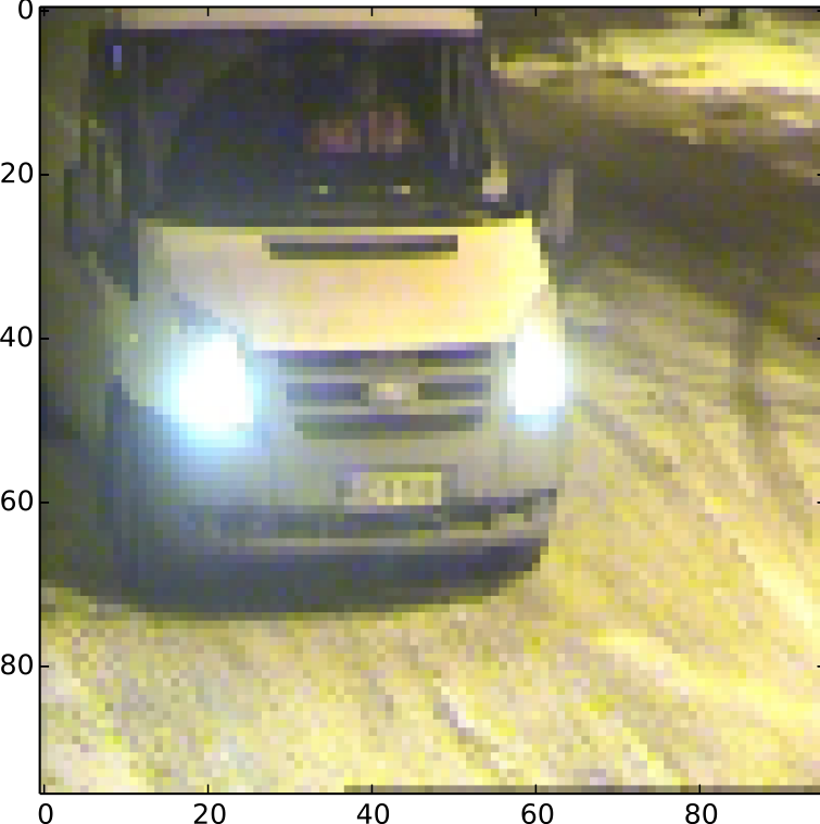
Figure 1: Example images from the two cameras. The images are downscaled to $96\times 96$ pixels to illustrate the network input resolution.

Our approach compares two data driven frameworks: a deep neural network and a support vector machine with Scale-Invariant Feature Transform (SIFT) image features. In other words, the proposed methods require no preprocessing except straightforward brightness normalization. The obvious benefits of such an approach are due to the simplicity of the implementation.

All the approaches found in the literature concentrate on recognition from still images. However, a typical access control setup extracts individual frames from a video stream for recognition. In this paper, we also limit our study to individual shots from the stream, but deep neural networks can be extended to process temporal video streams, as well. A straightforward approach is to compute the likelihoods for each car type for a number of video frames. Computing the average (or maximum) of these likelihoods tends to improve the accuracy of recognition, since a larger number of frames has a higher probability of a good frontal view of the vehicle (avoiding e.g, cases with car shown only partially, blocked by another vehicle or changing the lane). Alternatively, the temporal stack of video frames can be fed to a deep network directly; see, e.g., Tran et al. for categorization of sports activities [6].

TABLE I: Hyperparameters randomized over the iterations. The rightmost column describes the best configuration found within the 50 randomly selected configurations (see text).

Hyperparameter	Range	Selected Value
Number of Convolutional Layers	1 – 4	2
Number of Dense Layers	0 – 2	2
Input Image Size	{64, 96, 128, 160}	96
Kernel Size on All Convolutional Layers	{5, 9, 13, 17}	5
Number of Convolutional Maps	{16, 32, 48}	32
Learning rate	$10^{-5}$ – $10^{-1}$	0.001643

The remainder of this paper is organized as follows. Section II describes the proposed method in detail and in Section III, we report the experimental results and the image database used for experiments. Finally, Section IV will discuss the results and draw conclusions for future work.

II Materials and Methods

In this Section we will describe two data driven alternatives for car type recognition. The first one represents a deep architecture and the second a shallow one. Before describing the architectures, we describe the data used later in the experiments.

II-A Data

The database used in this paper was collected in collaboration with the company Visy Oy, whose license plate recognition based access control system installations have gathered tens of millions of vehicle images over the years. Each access control checkpoint is equipped with a digital PAL resolution camera, infrared illumination and a ground loop for detection of the vehicle in front of the camera.

The database consists of altogether 6555 vehicle images. The database was collected at two entrance gates at an access control system installation in a port in Finland. The pictures were acquired at interlaced PAL image resolution of $768\times 288$ per field. The images were extrapolated to the correct aspect ratio and resolution $768\times 576$. Examples of images from the database are shown in Figure 1, downscaled to the DNN input resolution of $96\times 96$.

We experimented with two installation scenarios: In the first case, the database consists of all images from one checkpoint and one camera. In this case the background is relatively steady and cars enter from approximately the same direction and angle. Note, however, that the images are collected over a long period of time, and there are significant changes in the environmental conditions (rain, snow, day/night). This experiment investigates the performance for an individual gate installation, which would always be calibrated (trained) individually.

The another scenario is more realistic, in that the database consists of images from two cameras at two different entrance checkpoints. Thus, the cars are entering at different angles from different directions and the background is not constant. This way we can also determine whether the methods learn the appearance of the background or the appearance of the actual vehicle. Namely, it could be possible that the classifier would learn to recognize small cars by spotting the background, which is not visible when blocked by a large vehicle.

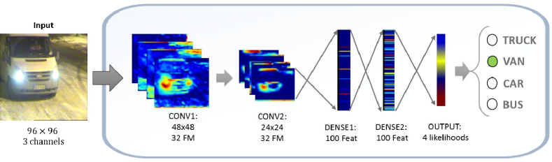
Figure 2: The structure of the proposed network. The network consists of altogether four hidden layers: two convolutional layers followed by two dense layers and an output layer.

II-B Deep Architecture: Deep Neural Networks

This decade has seen a breakthrough in image classification due to the advances in large neural networks. Several factors have contributed to their enormous success, including both the explosion of computational power brought by current Graphics Processing Units (GPU’s), and theoretical advances in neural network community, that have enabled the training of networks with very large number of stacked layers (Deep Neural Networks; DNN’s).

TABLE II: Accuracy of classification for the proposed methods. The experiments are done for two cases: A dataset consisting of pictures from a single camera angle, and a second dataset with pictures from two cameras with difference camera angles.

Classifier	Accuracy	#vehicles
Deep Neural Network (1 camera)	98.06 %	1500
SIFT + SVM (1 camera)	97.35 %	1500
Deep Neural Network (2 cameras)	97.75 %	6555
SIFT + SVM (2 cameras)	96.19 %	6555
Kafai et al. [3]	95.7 %	177
Zhang et al. [4]	95 %	2800
de S. Matos et al. [5]	69 %	100

Among the most significant highlights are achievements such as the large scale image classification record with the ImageNet database [7], the DeepFace face recognition method by Facebook [8] and the deep network learning to play computer games by Google [9]. Over the years, networks have grown in depth, ultimately reaching depths of 20-30 layers; see e.g., the 22-layer GoogLeNet [10] reaching the state-of-the art of the ImageNet Large-Scale Visual Recognition Challenge 2014 (ILSVRC 2014). There are several software platforms, where training and classification of a deep neural network are straightforward engineering tasks: These include Torch7 [11], Keras [12] and Caffe [13]. In our work, we will use the latter platform due to its particular efficiency for image data.

The key benefit of adding layers to the network is that this enables the classifier to learn higher lever structures within the image. For our particular problem, the network might have the ability to learn the appearance of the headlights on the first layer, their relative positions and distance on the second layer, and their relative location with respect to the car license plate on the third convolutional layer. In other words, the key to success is that the network can learn the feature extraction step in an optimal manner and can avoid the need for manual feature engineering; a critically important step in most earlier car type recognition approaches [3, 4, 5].

As a drawback of the deep neural network, there is a need to define the hyperparameters of the network. The choices of the number of layers, number of nodes, sizes of convolutional kernels, etc. all have a crucial importance on the resulting accuracy. For this problem, we follow the approach of Bergstra et al. [14], which randomly searches for a good combination of selected hyperparameters. The authors were able to show that as few as 8 or 16 iterations with random selection of hyperparameters can outperform both manual search and grid search with the same computational budget.

In our case, the hyperparameters randomized in search for the best network topology are summarized in Table I. The first two items define the depth of the network: The structure always consists of 1-4 convolutional layers followed by 0-2 dense layers. The input images are resized to square shape with dimensions within the range 64-160. The image size is closely related to the size of the convolutional kernels. We limit these to be equal in size on all layers within the range 5-17 pixels along both axes. The penultimate parameter of Table I defines the number of convolutional maps (i.e., the number of filters learned at each layer), and can change between 16-48 maps. Finally, a crucial parameter to the performance is the learning rate for the stochastic gradient backpropagation. This parameter is randomly sampled from a geometric distribution between $10^{-5}$ – $10^{-1}$. The rightmost column of Table I tabulates the selected hyperparameters in the experiments of Section III, after training a network with 50 randomly selected hyperparameter combinations.

The corresponding network topology is illustrated in Figure 2. In summary, our car type recognition network consists of five layers; two convolutional layers followed by two dense layers and an output layer. The first convolutional layer maps the three-channel $96\times 96$ input into 32 feature maps which are max-pooled to $48\times 48$ resolution. The second convolutional layer produces another 32 feature maps which are then downsampled to $24\times 24$ with max-pooling. After the convolutional layers, there are two fully connected layers with 100 nodes each. Finally, the output layer maps the 100 features on the last dense layer into four class likelihoods via a softmax operator. Between each layer, there is additionally a combination of a Dropout regularizer and a Rectified Linear Unit (ReLU) nonlinearity.

II-C Shallow Architecture: Support Vector Machine

For comparison, we also employ a conventional shallow method: Dense SIFT [15] and support vector machines (SVM) [16], which is a widely adopted combination in various frameworks for visual recognition such as fine-grained pet classification [17] and large-scale image categorization [18].

We adopt a bag-of-words model [19], whose visual words are generated densely by extracting SIFT descriptors [20] on the grids of images. The hyperparameter setting of dense SIFT follows that of [17], which adopts a stride of 6 pixels and at 4 scales (i.e., the spatial range of bins are 4, 6, 8, and 10 pixels). For incorporating spatial information, we use a spatial pooling method [21], which divides the whole image region into $1\times 1$ and $2\times 2$ cells. For each cell, SIFT descriptors are quantized into a 1000-clusters vocabulary by K-means clustering. As a result, we have a 5000-dimensional feature vector, whose histogram bins are normalized by $\ell_{1}$ norm, to represent each image. With the resulting image feature representation and the corresponding car type labels, a multiclass support vector machine using the RBF kernel is applied during training. For an unseen image, the image feature is fed into the trained support vector machines to classify its car type.

III Experiments

In this section we study the accuracy of the two classification methods in Sections II-B and II-C.

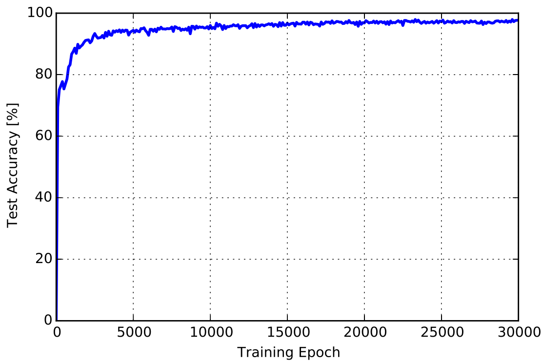
Figure 3: The learning curve of the network.

In order to assess the accuracies, the database described in Section II-A was split into a training set (90 % of all samples) and a test set (10% of all samples) in a stratified manner.

The learning curve of the proposed neural network is shown in Figure 3, which shows the classifier accuracy for the test data. The training is continued for 30,000 epochs without any accuracy related stopping criterion. The curve clearly shows that the dropout regularization and data augmentation are effective in avoiding overlearning. Moreover, a good classification accuracy is reached already at 15,000 iterations. In total, the training takes approximately 20 minutes on a NVidia Tesla K40t GPU.

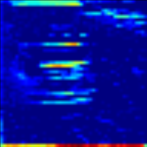
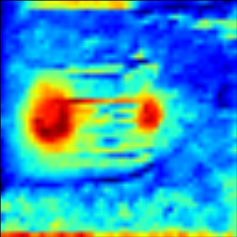
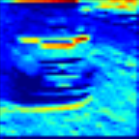
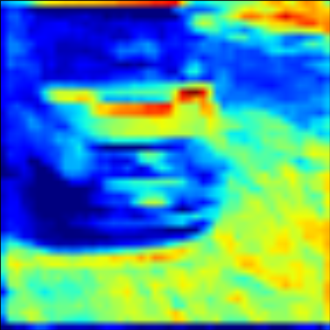
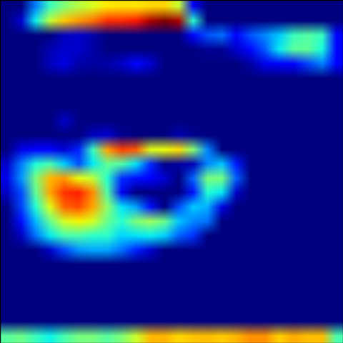
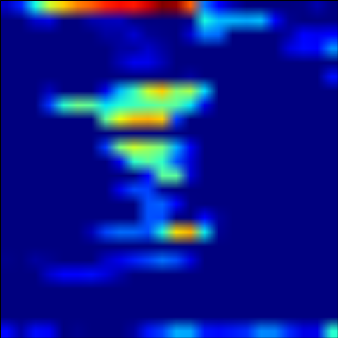
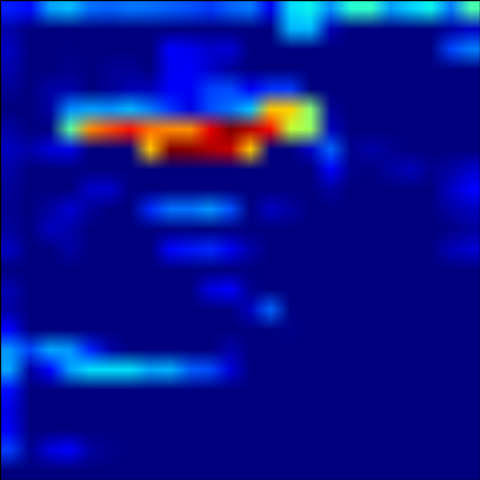
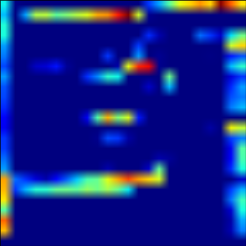
Figure 4: Examples of feature maps of the first (top row) and second (bottom row) convolutional layers computed from image at the right of Figure 1.

The results of the experiments are summarized in Table II. The first four rows describe the test set accuracies of the proposed methods for the single-camera and the two-camera cases. One can clearly see that both proposed approaches are relatively accurate in their recognition. However, in both cases the DNN is superior to the shallow architecture, although the margin is not particularly large. In fact, the results suggest that the car type recognizer uses relatively simple features as a basis of detection. Also the feature maps of the DNN shown in Figure 4 indicate that the convolutional layers learn to highlight image patterns that distinguish car types from each other: grille pattern, grille shape, headlight shape, etc. Possibly the added accuracy of the deep architecture is due to the higher level features, such as the distance of headlights and so on. Note that although the difference in accuracies may appear small, the DNN in fact makes over 40% fewer errors than the SVM in the two-camera case. Moreover, a visual inspection of the erroneous classifications show that the problems arise with vehicles ”between two classes” difficult even for humans to categorize, such as small vans, ambulances, etc.

The proposed methods are also compared to other approaches in Table II. Although the database in each paper is separate, the numbers indicate that the proposed method exceed the state of the art. In particular, the size of the database in our case is larger than that of the other experiments thus increasing our belief that data driven approaches are more reliable than manually engineered feature extraction pipelines [3, 4, 5].

We do acknowledge that the comparison would be more appropriate using the same database for all the methods. However, the datasets are unfortunately not public, and the implementation of the alternative (relatively tailored) methods in exactly the original manner is a non-trivial task. However, as our database is among the largest, we have a strong belief that the proposed data-driven approaches would be successful with the other datasets, as well. To facilitate later comparison in a reproducible manner, we provide the details of our network (topology and pretrained coefficients) at the supplementary site for the paper.

The erroneous recognition results are often related to ambiguous annotation. Three examples of incorrectly classified results are shown in Figure 5. In all cases, the vehicles are categorized as ”normal vehicle” instead of the annotated category ”van”. In fact, they all represent a small van, which has resemblance to both categories and are slightly difficult to categorize unambiguously.

IV Conclusions

In this paper we studied the use of data driven image recognition techniques for car type classification. This separates the work from existing approaches that rely on an elaborate manually engineered feature extraction pipeline, thus simplifying the software architecture substantially. It was shown that both studied methods (Deep neural network and SVM with SIFT features) are able to accurately recognize the car type, and the DNN is superior in accuracy to the SVM.

It was also shown that both proposed methods outperform methods of the earlier studies. However, one should bear in mind that the image databases in these studies were different and not directly comparable with each other. In fact, one our our future plans is to extend our work towards freely available image databases [22, 23]. However, this will require manual annotation of the databases, as the current annotations only include the car make.

An interesting question is how well the trained models generalize to novel situations, such as new traffic lanes with slightly different viewing angle, illumination or direction of traffic. In this paper we have shown that a single model can learn to recognize vehicles on two lanes with highly varying illumination. Thus, there is no reason why the network would not generalize to further installations. However, the study of how many lanes need to be labeled manually in order to generalize to any environment is left for future work on the topic.

Figure 5: Examples of vehicles incorrectly classified by the network. All three are assigned to category van, although they are annotated as normal vehicle.

V Acknowledgements

The authors would like to acknowledge CSC - IT Center for Science Ltd. for computational resources.

References

- [1] E. Hsiao, S. Sinha, K. Ramnath, S. Baker, L. Zitnick, and R. Szeliski, “Car make and model recognition using 3d curve alignment,” in Applications of Computer Vision (WACV), 2014 IEEE Winter Conference on, March 2014, pp. 1–1.
- [2] L. Dlagnekov and S. J. Belongie, Recognizing cars. Department of Computer Science and Engineering, University of California, San Diego, 2005.
- [3] M. Kafai and B. Bhanu, “Dynamic bayesian networks for vehicle classification in video,” Industrial Informatics, IEEE Transactions on, vol. 8, no. 1, pp. 100–109, 2012.
- [4] B. Zhang, Y. Zhou, and H. Pan, “Vehicle classification with confidence by classified vector quantization,” Intelligent Transportation Systems Magazine, IEEE, vol. 5, no. 3, pp. 8–20, 2013.
- [5] F. M. de S. Matos and R. M. C. R. de Souza, “Hierarchical classification of vehicle images using nn with conditional adaptive distance,” in Neural Information Processing, ser. Lecture Notes in Computer Science, M. Lee, A. Hirose, Z.-G. Hou, and R. Kil, Eds. Springer Berlin Heidelberg, 2013, vol. 8227, pp. 745–752.
- [6] D. Tran, L. Bourdev, R. Fergus, L. Torresani, and M. Paluri, “Learning spatiotemporal features with 3d convolutional networks,” in Proceedings of the IEEE International Conference on Computer Vision, 2015, pp. 4489–4497.
- [7] A. Krizhevsky, I. Sutskever, and G. E. Hinton, “Imagenet classification with deep convolutional neural networks,” in Advances in neural information processing systems, 2012, pp. 1097–1105.
- [8] Y. Taigman, M. Yang, M. Ranzato, and L. Wolf, “Deepface: Closing the gap to human-level performance in face verification,” in 2014 IEEE Conference on Computer Vision and Pattern Recognition (CVPR). IEEE, 2014, pp. 1701–1708.
- [9] V. Mnih, K. Kavukcuoglu, D. Silver, A. A. Rusu, J. Veness, M. G. Bellemare, A. Graves, M. Riedmiller, A. K. Fidjeland, G. Ostrovski et al., “Human-level control through deep reinforcement learning,” Nature, vol. 518, no. 7540, pp. 529–533, 2015.
- [10] C. Szegedy, W. Liu, Y. Jia, P. Sermanet, S. Reed, D. Anguelov, D. Erhan, V. Vanhoucke, and A. Rabinovich, “Going deeper with convolutions,” arXiv preprint arXiv:1409.4842, 2014.
- [11] R. Collobert, K. Kavukcuoglu, and C. Farabet, “Torch7: A matlab-like environment for machine learning,” in BigLearn, NIPS Workshop, no. EPFL-CONF-192376, 2011.
- [12] F. Chollet, “Keras deep learning library,” https://github.com/fchollet/keras, 2016.
- [13] Y. Jia, E. Shelhamer, J. Donahue, S. Karayev, J. Long, R. Girshick, S. Guadarrama, and T. Darrell, “Caffe: Convolutional architecture for fast feature embedding,” in Proceedings of the ACM International Conference on Multimedia. ACM, 2014, pp. 675–678.
- [14] J. Bergstra and Y. Bengio, “Random search for hyper-parameter optimization,” The Journal of Machine Learning Research, vol. 13, no. 1, pp. 281–305, 2012.
- [15] A. Vedaldi and B. Fulkerson, “VLFeat: An open and portable library of computer vision algorithms,” http://www.vlfeat.org/, 2008.
- [16] C. Cortes and V. Vapnik, “Support-vector networks,” Machine learning, vol. 20, no. 3, pp. 273–297, 1995.
- [17] O. M. Parkhi, A. Vedaldi, A. Zisserman, and C. V. Jawahar, “Cats and dogs,” in IEEE Conference on Computer Vision and Pattern Recognition, 2012.
- [18] K. Chatfield, V. Lempitsky, A. Vedaldi, and A. Zisserman, “The devil is in the details: an evaluation of recent feature encoding methods,” in British Machine Vision Conference, 2011.
- [19] G. Csurka, C. Dance, L. Fan, J. Willamowski, and C. Bray, “Visual categorization with bags of keypoints,” in Workshop on statistical learning in computer vision, ECCV, vol. 1, no. 1-22. Prague, 2004, pp. 1–2.
- [20] D. G. Lowe, “Object recognition from local scale-invariant features,” in Computer vision, 1999. The proceedings of the seventh IEEE international conference on, vol. 2. Ieee, 1999, pp. 1150–1157.
- [21] S. Lazebnik, C. Schmid, and J. Ponce, “Beyond bags of features: Spatial pyramid matching for recognizing natural scene categories,” in Computer Vision and Pattern Recognition, 2006 IEEE Computer Society Conference on, vol. 2. IEEE, 2006, pp. 2169–2178.
- [22] L. Yang, P. Luo, C. C. Loy, and X. Tang, “A large-scale car dataset for fine-grained categorization and verification,” in Proceedings of the IEEE Conference on Computer Vision and Pattern Recognition, 2015, pp. 3973–3981.
- [23] J. Krause, M. Stark, J. Deng, and L. Fei-Fei, “3d object representations for fine-grained categorization,” in Computer Vision Workshops (ICCVW), 2013 IEEE International Conference on. IEEE, 2013, pp. 554–561.