Spontaneous Spin Textures in Multiorbital Mott Systems

Abstract

Spin textures in $\mathbf{k}$-space arising from spin-orbit coupling in non-centrosymmetric crystals find numerous applications in spintronics. We present a mechanism that leads to appearance of $\mathbf{k}$-space spin texture due to spontaneous symmetry breaking driven by electronic correlations. Using dynamical mean-field theory we show that doping a spin-triplet excitonic insulator provides a means of creating new thermodynamic phases with unique properties. The numerical results are interpreted using analytic calculations within a generalized double-exchange framework.

Manipulation of spin polarization by controlling charge currents and vice versa has attracted considerable attention due to applications in spintronic devices. A major role is played by spin-orbit (SO) coupling in non-centrosymmetric systems. As originally realized by Dresselhaus Dresselhaus (1955) and Rashba Rashba (1960), SO coupling in a non-centrosymmetric crystal lifts the degeneracy of the Bloch states at a given $\mathbf{k}$-point and locks their momenta and spin polarizations together giving rise to a spin texture in reciprocal space. This leads to a number of phenomena Manchon et al. (2015) such as spin-torques in ferro- Manchon and Zhang (2008); Li et al. (2015) and anti-ferromagnets Železný et al. (2014); Wadley et al. (2016), topological states of matter, or spin textures in the reciprocal space that are the basis of the spin galvanic effect. Wunderlich et al. (2009) Electronic correlations alone can provide coupling between spin polarization and charge currents, e.g., via effective magnetic fields acting on electrons moving through a non-coplanar spin background. Nagaosa et al. (2012); Jonietz et al. (2010) Wu and Zhang Wu and Zhang (2004) proposed that SO coupling can be generated dynamically in analogy to the breaking of relative spin-orbit symmetry in ³He Vollhardt and Wölfle (2013). Subsequently, an effective field theory of spin-triplet Fermi surface instabilities with high orbital partial wave was developed in Ref. Wu et al., 2007.

Here, we present a spontaneous formation of a $\mathbf{k}$-space spin texture, similar to the effect of Rashba-Dresselhaus SO coupling, in centrosymmetric bulk systems with no intrinsic SO coupling. The spin texture is a manifestation of excitonic magnetism that has been proposed to take place in some strongly correlated materials. Khaliullin (2013); Kuneš and Augustinský (2014a) The basic ingredient is a crystal built of atoms with quasi-degenerate singlet/triplet ground states. Under suitable conditions a spin-triplet exciton condensate Halperin and Rice (1968); Balents (2000) is formed, which may adopt a variety of thermodynamic phases with diverse properties Kuneš (2015). Several experimental realizations of excitonic magnetism have already been discussed in the literature. Kuneš and Augustinský (2014b); Cao et al. (2014); Jain et al. ; Dey et al. (2016); Pajskr et al. (2016)

Model. We use the dynamical mean-field theory (DMFT) to study the minimal model of an excitonic magnet – the two-orbital Hubbard Hamiltonian at half-filling

$$\begin{split}&H=\sum_{\langle ij\rangle}H_{t}^{(ij)}+\frac{\Delta}{2}\sum_{i\sigma}\left(n^{a}_{i\sigma}-n^{b}_{i\sigma}\right)+\sum_{i}H^{(i)}_{\text{int}}\\ &H^{(i)}_{\text{int}}=U\left(n^{a}_{i\uparrow}n^{a}_{i\downarrow}+n^{b}_{i\uparrow}n^{b}_{i\downarrow}\right)+U^{\prime}\sum_{\sigma\sigma^{\prime}}n^{a}_{i\sigma}n^{b}_{i\sigma^{\prime}}\\ &-J\sum_{\sigma}\left(n^{a}_{i\sigma}n^{b}_{i\sigma}+\gamma a_{i\sigma}^{\dagger}a_{i-\sigma}^{\phantom{\dagger}}b_{i-\sigma}^{\dagger}b_{i\sigma}^{\phantom{\dagger}}\right).\end{split}$$ (1)

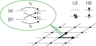
Figure 1: The hopping processes with corresponding amplitudes on the square lattice. The parameters used in the calculations: $t_{a}=0.4118$, $t_{b}=-0.1882$, $V_{1}=\pm V_{2}=0.05$, $\Delta=3.4$, $U=4$, $U^{\prime}=2$, and $J=1$ in the units of eV.

The local part of the Hamiltonian contains the crystal-field splitting $\Delta$ between the orbitals labeled $a$ and $b$ and the Coulomb interaction with ferromagnetic Hund’s exchange $J$. The kinetic part $H_{t}$ describes the nearest-neighbor hopping on the square lattice between the same orbital flavors $t_{a},t_{b}$ as well as cross-hopping between the different orbital flavors $V_{1},V_{2}$, see Fig. 1. The parameters $\Delta$ and $J$ are balanced such that the energy difference between the atomic low-spin (LS) and high-spin (HS) states is smaller or comparable to the kinetic energy gain due to the electron delocalization. The numerical simulations using continuous-time quantum Monte-Carlo impurity solver Werner et al. (2006); Albuquerque et al. (2007) were performed with the density-density approximation for the interaction ($\gamma=0$), which effectively introduces a magnetic easy axis in the present model. Analytic mean-field calculations as well as preliminary DMFT computations performed with SU(2) symmetric model Kuneš (2015) show only quantitative differences (e.g. reduction of the transition temperature). The spectral functions were obtained using the maximum entropy method. Gubernatis et al. (1991) Technical details can be found in the Supplemental Material (SM).

Studies Kuneš and Augustinský (2014a, b); Kuneš (2014); Kaneko and Ohta (2014); Kaneko et al. (2015); Hoshino and Werner performed without cross-hopping $V_{1,2}=0$ revealed formation of the exciton condensate below a critical temperature, which decreases with doping away from integer filling. In the strong-coupling limit the ground state wave function of a uniform condensate can be approximated by a product of local functions $\Pi_{i}|C_{i}\rangle$ with each ${|C\rangle=sb_{\uparrow}^{\dagger}b_{\downarrow}^{\dagger}+\xi_{1}a_{\uparrow}^{\dagger}b_{\uparrow}^{\dagger}+\tfrac{\xi_{0}}{\sqrt{2}}(a_{\uparrow}^{\dagger}b^{\dagger}_{\downarrow}+a_{\downarrow}^{\dagger}b^{\dagger}_{\uparrow})+\xi_{-1}a_{\downarrow}^{\dagger}b_{\downarrow}^{\dagger}|\text{v}\rangle}$ , describing a local hybrid between LS and HS states with amplitudes $s$, $\xi_{1}$, $\xi_{0}$, and $\xi_{-1}$, which provides a useful analytic reference for interpretation of the numerical results. In the DMFT calculations we characterise the thermodynamic phases by the order parameter ${\bm{\phi}^{(i)}=\sum_{\alpha\beta}\bm{\sigma}_{\alpha\beta}\langle a_{i\alpha}^{\dagger}b_{i\beta}^{\phantom{\dagger}}\rangle}$, with Pauli matrices $\bm{\sigma}$. In addition, we evaluate the spin moment per atom $\mathbf{M}$ as well as the spin density in the direct space $\mathbf{m}(\mathbf{r})$  and in the reciprocal space ${\mathbf{m}_{\mathbf{k}}=\sum_{\alpha\beta}\bm{\sigma}_{\alpha\beta}\langle a_{\mathbf{k}\alpha}^{\dagger}a_{\mathbf{k}\beta}^{\phantom{\dagger}}+b_{\mathbf{k}\alpha}^{\dagger}b_{\mathbf{k}\beta}^{\phantom{\dagger}}\rangle}$.

In Fig. 2 we show the phase diagrams of (1) as functions of temperature $T$ and hole doping $n_{h}$ away from $n=2$. We choose the hopping parameters so that $t_{a}t_{b}<0$ which leads to a uniform $\bm{\phi}$-order. Note that on a bipartite lattice the $t_{a}t_{b}>0$ case with a staggered $\bm{\phi}$-order can be mapped on the $t_{a}t_{b}<0$ by the gauge transformation $a_{i}\rightarrow(-1)^{i}a_{i}$. Kuneš (2015) We consider two cross-hopping patterns at this point: $V_{1}=V_{2}$ (even) and $V_{1}=-V_{2}$ (odd). The two corresponding phase diagrams share the general features inherited from the ’parent’ system with no cross-hopping studied in Kuneš, 2014. These include the polar state with no ordered moments at low doping levels and a doping-induced transition to a different excitonic phase. The thermodynamic phase can be distinguished by several criteria. The ferromagnetic condensate (FMEC) has the oder parameter of the form $\bm{\phi}=\mathbf{x}+i\mathbf{x}^{\prime}$ (with non-collinear real vectors $\mathbf{x}$ and $\mathbf{x}^{\prime}$), which generates a finite uniform polarization $M_{\perp}$ perpendicular to $\bm{\phi}$. The order parameter in polar condensates can be written as $\bm{\phi}=e^{i\varphi}\mathbf{x}$ (real vector $\mathbf{x}$ times an arbitrary scalar phase $\varphi$). The polar condensates can be further distinguished by their time-reversal (TR) symmetry into the spin-density-wave (SDW; real $\bm{\phi}$; breaks TR) and spin-current-density-wave (SCDW; imaginary $\bm{\phi}$; preserves TR) types, introduced by Halperin and Rice, Halperin and Rice (1968). The SDW order gives rise to a finite intra-atomic spin polarization $\mathbf{m}(\mathbf{r})$ –higher magnetic multipole– while the SCDW order gives rise to intra-atomic spin current with $\mathbf{m}(\mathbf{r})=0$.  The preference of the undoped system for SDW or SCDW ordering on a given bond is controlled by the sign of $t_{a}t_{b}V_{1}V_{2}$ and follows the rules given in Ref. Kuneš and Augustinský, 2014a. Finally, we distinguish the polar phases into the primed and unprimed ones. The spin(current)-polarization in the unprimed phases is purely local, reflected by $\mathbf{m}_{\mathbf{k}}=0$. The primed phase are characterized by appearance of $\mathbf{k}$-space spin textures, $\mathbf{m}_{\mathbf{k}}\neq 0$, which in case of SCDW’ phase represents global spin currents. The characteristics for the different phases are summarized in Table 1.

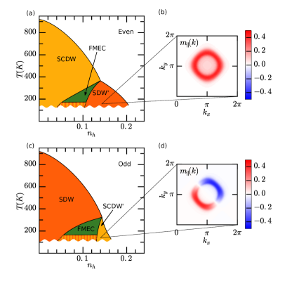
Figure 2: (a) and (c): Phase diagrams in the doping-temperature plane for even and odd cross-hopping, respectively. Full lines mark continuous transitions, dotted lines mark the boundaries of phase coexistence regions. (b) and (d): The spin textures at the indicated points of the phase diagrams in the units of $\mu_{B}(\frac{a_{0}}{2\pi})^{2}$ obtained for $n_{h}$=0.14 at $T$=193 K.

Table 1: The characteristics of different condensate phases: $M_{\perp}$ and $M_{\parallel}$ is magnetic moment per atom perpendicular and parallel to the order parameter $\bm{\phi}$, respectively; $\mathbf{m}(\mathbf{r})$ and $\mathbf{m}_{\mathbf{k}}$ are the spin densities in direct and reciprocal space, respectively. By ✓/0 we indicate that both cases may be realized (see the text).

Condensate state	$M_{\perp}$	$M_{\parallel}$	$\mathbf{m}(\mathbf{r})$	$\mathbf{m}_{\mathbf{k}}$	$\operatorname{Re}\bm{\phi}$	$\operatorname{Im}\bm{\phi}$
FMEC	✓	✓/0	✓	✓	✓	✓
SDW	0	0	✓	0	✓	0
SCDW	0	0	0	0	0	✓
SDW’	0	✓/0	✓	✓	✓	0
SCDW’	0	0	0	✓	0	✓

Double-exchange mechanism. Observation of the spontaneous spin textures in the primed phases is our central result. It can be understood by invoking the generalized double-exchange mechanism, recently used by Chaloupka and Khaliullin to study ruthenates. Chaloupka and Khaliullin (2016) Analogous to the well-known Zener double-exchange Zener (1951) in manganites, the exciton condensate acts as a filter for propagation of doped carriers. The stable phase is determined by the competition between the kinetic energy of doped carriers and the energy difference between possible condensates. In the strong coupling limit, propagation of a single electron through the condensate with order parameter $\bm{\phi}^{(i)}$ is described by an effective Hamiltonian (see SM for the derivation)

$$\begin{split}H_{\text{eff}}=&\sum_{\langle ij\rangle}\left(t_{s}\delta_{\alpha\beta}+\frac{1}{2}\mathbf{B}^{(ij)}\cdot\bm{\sigma}_{\alpha\beta}\right)\tilde{b}^{\dagger}_{i\alpha}\tilde{b}^{\phantom{\dagger}}_{j\beta}+\text{h.c.}\\ \text{with}\\ \mathbf{B}^{(ij)}=&\frac{it_{a}}{2s^{2}}\left(\bm{\phi}^{(j)}\wedge{\bm{\phi}^{(i)}}^{*}\right)+V_{1}^{(ji)}\bm{\phi}^{(j)}+V_{2}^{(ji)}{\bm{\phi}^{(i)}}^{*}\end{split}$$ (2)

and $t_{s}=-t_{b}s^{2}-t_{a}\left(1-s^{2}\right)$. Here, $\bm{\sigma}$ are the Pauli matrices and $s^{2}$ is the LS fraction in the condensate. In general, the $\mathbf{B}$-fields depend in the site indices as indicated in the brackets - in the studied ’odd’ and ’even’ models the site indices are obsolete.

The $\phi$-quadratic term in (2) describes the standard double-exchange interaction of the doped particle with the uniform background with spin polarization $\mathbf{M}_{\perp}=-i\left(\bm{\phi}^{*}\wedge\bm{\phi}\right)/s^{2}$.  At low doping the anti-ferromagnetic interactions between the HS states dominate, rendering the system a polar condensate with spin-independent hopping in (2). For some critical doping, however, the gain in the kinetic energy of doped carriers in FMEC outweighs the cost in the HS-HS exchange energy and the system adopts the FMEC state.

The $\phi$-linear term in (2), which dominates at least close to the normal-phase boundary, appears only with finite cross-hopping in the condensate phase. The strong coupling calculations Kuneš and Augustinský (2014a) (see SM) show that the $V_{1}$ and $V_{2}$ contributions in (2) cancel out, $V_{1}\bm{\phi}+V_{2}\bm{\phi}^{*}=0$, for $\bm{\phi}$ that minimizes the bond energy. On a bipartite lattice, where all bonds can be satisfied simultaneously, the $\phi$-linear term vanishes globally allowing the SDW and SCDW phases at finite doping.

When kinetic energy gain of the doped particles overcomes the interactions selecting the condensate type in the undoped system, the $\phi$-linear term in (2) becomes finite. It has a form of an exchange field acting on bonds or equivalently acting locally in the reciprocal space, which for the two hopping patterns considered so far reads

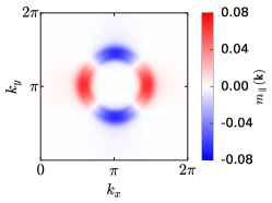
Figure 3: The $d$-wave spin texture in the SDW’ phase of a model with even cross-hopping of opposite signs along the $x$ and $y$ axes. The result shown here were obtained for $n_{h}=0.16$ at $T$=193 K.

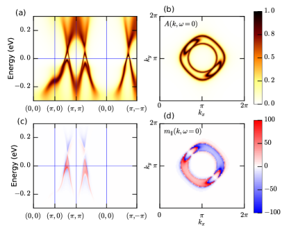
Figure 4: One-particle spectral density in SCDW’ phase for the same parameters as Fig. 2d: (a) total spectral density $A(\mathbf{k},\omega)$ along high-symmetry lines in the Brillouin zone, (b) the Fermi surface ${A(\mathbf{k},\omega=0)}$, (c) in-plane magnetization spectral density $m_{\parallel}(\mathbf{k},\omega)$ along the same lines as in panel (a), (d) in-plane magnetization density at the Fermi level ${m_{\parallel}(\mathbf{k},\omega=0)}$ in the units of $\mu_{B}.$eV${}^{-1}(\frac{a_{0}}{2\pi})^{2}$.

$$\mathbf{B}_{\mathbf{k}}=4V_{1}\bm{\phi}\begin{cases}\cos k_{x}+\cos k_{y}&\text{SDW'}\\ i(\sin k_{x}+\sin k_{y})&\text{SCDW'}\end{cases}\\$$ (3)

More generally, the $\mathbf{B}_{\mathbf{k}}$ reflects the symmetry of the cross-hopping pattern. The $s$-wave symmetry of our even cross-hopping therefore leads to an $s$-wave texture, Fig. 2, with a finite $M_{\parallel}$. Apart from strong radial localization, the $\mathbf{m}_{\mathbf{k}}$ is not qualitatively different from an approximately constant $\mathbf{m}_{\mathbf{k}}$ of normal local moment ferromagnet. However, a $d$-wave cross-hopping, with $V$’s along the $x$ and $y$ directions having opposite sings, produces a $d$-wave texture, shown in Fig. 3, and $M_{\parallel}=0$. We point out that without doping the $s$- and $d$-wave systems are identical, in the strong-coupling limit, since the cross-hopping enters as a product $V_{1}V_{2}$ on each bond. Kuneš and Augustinský (2014a)

The SCDW’ phase is characterized by purely imaginary $\bm{\phi}$ which gives rise to $\mathbf{k}$-odd exchange field in (3). The odd cross-hopping pattern can be thought of as having $p_{x}+p_{y}$ symmetry, which is imprinted in the spin texture, shown in Fig. 2b. There is not only no net polarization $\mathbf{M}=0$, but the polarization is zero in every point $\mathbf{m}(\mathbf{r})=0$ reflecting the TR invariance of the SCDW’ state. In Fig. 4 we analyze spin texture in the SCDW’ state in detail. The frequency-resolved contributions to $\mathbf{m}_{\mathbf{k}}$ in Figs. 4c,d reveal that the spin polarization comes from a narrow energy range around the Fermi level. Spectral functions exhibit rather sharp quasi-particle bands around the Fermi level resembling a band structure of non-interacting system. The spin density, on the other hand, is quite different from that of non-interacting system. It cannot be associated with particular quasi-particle bands but rather lives on their tails in sharply defined regions of the Brillouin zone.

The shape of the spin texture in the SCDW’ state is determined by the model parameters. Its collinear polarization, similar to equal combination of Rashba and Dresselhaus SO coupling Manchon et al. (2015), is picked randomly at the transition. The Weiss field in the SCDW and SCDW’ phases, which generates local intra-atomic spin currents, can be viewed as spontaneously generated SO coupling. The corresponding ’SO’ splitting is approximately $(U-2J)|\phi|$ thus can be as large as lower units of eV. Only in the SCDW’ phase the spontaneous SO coupling is taken to the inter-atomic scale. The equivalent of Rashba/Dresselhaus SO coupling is found in (3) with the largest amplitude, in the (1,1) direction, of $4V_{1}|\phi|a_{0}$. With $|\phi|\sim 0.2-0.4$ (maximum theoretical value is $1/\sqrt{2}$), the present cross-hopping of 50 meV, and the lattice constant $a_{0}$ of a few $\AA$ the effective Rashba/Dresselhaus SO constant is of the order $1\times 10^{-11}$ eV m.

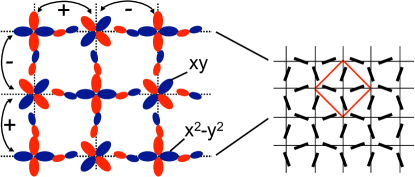
Figure 5: A cartoon view of the orbital pattern (left) that gives rise to $t_{a},t_{b}>0$ and$V_{1}=V_{2}$ on each bond with alternating signs between bonds (only half of the orbitals is shown for sake of clarity). Zoomed out view of the texture on the ligand sublattice (right). Red square marks the crystallographic unit cell. The model can be transformed to the ’odd’ cross-hopping case with a single-atom unit cell by sublattice transformation $a_{i}\rightarrow(-1)^{i}a_{i}$.

Realization. To support the SDW’ or SCDW’ states a material: (i) must exhibit spin-triplet polar exciton condensation, (ii) the local SDW or SCDW must give rise to spin-dependent hopping in Eq. 3, and (iii) the spin-dependent hopping must generate a global pattern spin polarization or spin currents.

Transition metal perovskites are the most discussed candidates for excitonic magnetism. Khaliullin (2013); Kuneš and Augustinský (2014b); Jain et al. The singlet-triplet quasi-degeneracy favorable for (i) is typically realized in $d^{6}$ configuration in octahedral geometry (Fe²⁺, Co³⁺, Ni⁴⁺), $d^{8}$ configuration in square planar geometry (Ni²⁺), or $d^{4}$ configuration in octahedral geometry with strong spin-orbit coupling (Ru⁴⁺, Os⁴⁺, Rh⁵⁺, Ir⁵⁺). Therefore we focus on models built of $d$-orbitals.

It is quite straightforward to construct the ’even’ (or $d$-wave) model and thus the SDW’ state from orbitals of the same parity. We focus on the more difficult ’odd’ model and the SCDW’ state. Here we have two options. First, we use the fact that only the in-plane parity is relevant. We can start with lattice of $3z^{2}-r^{2}$ (or $x^{2}-y^{2}$) and $z(x+y)$ orbitals. Breaking of the $z\leftrightarrow-z$ symmetry, e.g., by a substrate leads to the desired ’odd’ cross-hopping pattern.

Second option is a model built of $x^{2}-y^{2}$ and $xy$ orbitals with more than one atom in the unit cell. In this case, the conditions (ii) and (iii) become distinct. For example, one can obtain $V_{1}V_{2}<0$ on each bond by tilting the orbitals (oxygen octahedral in real perovskite). However, the corresponding pattern of $\mathbf{B}^{(ij)}$ has alternating signs and does not give rise to a finite $\mathbf{m}_{\mathbf{k}}$. In order, to create the desired cross-hopping pattern the inversion centered at the atomic site has to be removed. In Fig. 5 we show an example of such hopping pattern in Emery-like model. The diagonal hopping amplitudes $t_{a}$ and $t_{b}$ are both negative. The cross-hopping $(V_{1},V_{2})$ , via tilted oxygen orbitals (induced for example by a substrate with appropriate texture), follows the $(++),(--),(++),...$ pattern along both $x$ and $y$ directions. These suggestions are obviously not the only ways to realize hopping patterns favoring the SCDW’ phase.

The most advanced experimental realization of the triplet-excitonic condensation is perhaps the Ca₂RuO₄ Jain et al. described by the model of Khaliullin Khaliullin (2013), which is equivalent to the strong coupling limit of the present model for a special choice of parameters. While the double-exchange mechanism is active also in ruthenates Chaloupka and Khaliullin (2016), static spin textures were not reported. Since the equivalents of cross- and diagonal hopping in ruthenates originate from the same $t_{2g}\rightarrow t_{2g}$ process, their ratio is fixed and close to one. This is quite different from the present parameters with small cross-hopping.

Finally, we point out that $\mathbf{k}$-space spin textures are accessible in cold atoms experiments, where the two-orbital model may be sufficiently simple to realize.

In conclusion, we have presented the doping of exciton condensates in systems of strongly correlated electrons as a way to generate unique states of matter. The generalized double-exchange mechanism in these systems can give rise to exchange fields that act on the itinerant electrons in the reciprocal space. The actual existence of such fields depends on the particular thermodynamic phase and crystal symmetry. In the studied model we found a broken-symmetry state with a $\mathbf{k}$-space spin texture with a symmetry of an equal combination of Rashba and Dresselhaus SO couplings.

I Supplemental Material

I.1 Model and computational method

The model Hamiltonian reads

$$H^{(\mathbf{i},\mathbf{i}+\mathbf{e}_{\nu})}_{\text{t}}= \sum_{\sigma}\left(t_{a}a_{\mathbf{i}+\mathbf{e}_{\nu}\sigma}^{\dagger}a^{\phantom{\dagger}}_{\mathbf{i}\sigma}+t_{b}b_{\mathbf{i}+\mathbf{e}_{\nu}\sigma}^{\dagger}b^{\phantom{\dagger}}_{\mathbf{i}\sigma}\right)+H.c.$$ (4)

$$+ \sum_{\sigma}\left(V_{1}a_{\mathbf{i}+\mathbf{e}_{\nu}\sigma}^{\dagger}b^{\phantom{\dagger}}_{\mathbf{i}\sigma}+V_{2}b_{\mathbf{i}+\mathbf{e}_{\nu}\sigma}^{\dagger}a^{\phantom{\dagger}}_{\mathbf{i}\sigma}\right)+H.c.$$

$$H^{(\mathbf{i})}_{\text{loc}}= \frac{\Delta}{2}\sum_{\sigma}\left(n^{a}_{i\sigma}-n^{b}_{i\sigma}\right)$$

$$+ U\left(n^{a}_{\mathbf{i}\uparrow}n^{a}_{\mathbf{i}\downarrow}+n^{b}_{\mathbf{i}\uparrow}n^{b}_{\mathbf{i}\downarrow}\right)+U^{\prime}\sum_{\sigma\sigma^{\prime}}n^{a}_{\mathbf{i}\sigma}n^{b}_{\mathbf{i}\sigma^{\prime}}$$

$$- J\sum_{\sigma}\left(n^{a}_{\mathbf{i}\sigma}n^{b}_{\mathbf{i}\sigma}+\gamma a_{\mathbf{i}\sigma}^{\dagger}a_{\mathbf{i}-\sigma}^{\phantom{\dagger}}b_{\mathbf{i}-\sigma}^{\dagger}b_{\mathbf{i}\sigma}^{\phantom{\dagger}}\right).$$

where $\mathbf{e}_{\nu}$ stands for the lattice vector of 2D square lattice. The DMFT calculations were performed for the same parameters as in Ref. Kuneš, 2014: $U=4$, $J=1$, $U^{\prime}=U-2J$, $\Delta=3.4$, $t_{a}=0.4118$, $t_{b}=-0.1882$, $V_{1}=\pm V_{2}=0.05$, $\gamma=0$ (density-density approximation). We use eV as the energy units and give temperatures in K.

We used continuous time quantum Monte-Carlo impurity solver Werner et al. (2006) modified to treat real off-diagonal hybridization functions.

The spectra were obtained with maximum entropy analytic continuation Gubernatis et al. (1991) of the self-energy. For the off-diagonal elements, the spectral function of which is not positive definite, we used the ansatz ${S(\omega)=S_{+}({\omega})-S_{-}({\omega})}$, where $S_{+}(\omega)$ and $S_{-}(\omega)$ are positive definite. We checked that $S(\omega)$ obtained this way depends only weakly on the default model (while $S_{+}$ and $S_{-}$ are strongly default model sensitive).

In Fig. 6 we show the $\mathbf{k}$-resolved spectral function from Fig. 4 of the article over the full energy range.

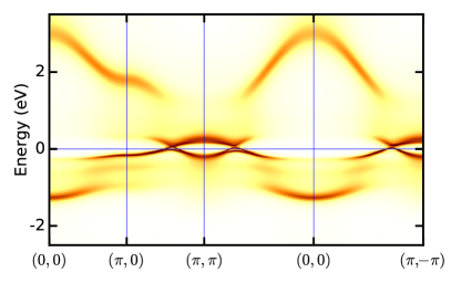
Figure 6: The spectral function over the full relevant energy range for the same parameters at in Fig. 3 of the main text.

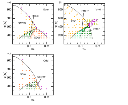
Figure 7: The input data for the Fig. 2 in the main text. The dots indicate the points at which actual calculation was performed.

I.2 Strong coupling limit

In the strong-coupling limit the on-site Hilbert space can be restricted to the states

$$\begin{split}&|\emptyset\rangle=b_{\uparrow}^{\dagger}b^{\dagger}_{\downarrow}|\text{v}\rangle,\\ &|1\rangle=a_{\uparrow}^{\dagger}b^{\dagger}_{\uparrow}|\text{v}\rangle,|0\rangle=\tfrac{1}{\sqrt{2}}(a_{\uparrow}^{\dagger}b^{\dagger}_{\downarrow}+a_{\downarrow}^{\dagger}b^{\dagger}_{\uparrow})|\text{v}\rangle,|-1\rangle=a_{\downarrow}^{\dagger}b^{\dagger}_{\downarrow}|\text{v}\rangle,\\ &|\uparrow\rangle=b_{\uparrow}^{\dagger}|\text{v}\rangle,|\downarrow\rangle=b_{\downarrow}^{\dagger}|\text{v}\rangle,\end{split}$$

where the bottom row corresponds to the doped hole states. The wave function of the uniform condensate can be written approximately as a product of local functions ${\Pi_{i}|C_{i}\rangle}$ with

$$\begin{split}&|C_{i}\rangle=s|\emptyset_{i}\rangle+\xi_{-1}^{(i)}|-1_{i}\rangle+\xi_{0}^{(i)}|0_{i}\rangle+\xi_{1}^{(i)}|1_{i}\rangle,\\ &s^{2}+|\xi_{1}^{(i)}|^{2}+|\xi_{0}^{(i)}|^{2}+|\xi_{-1}^{(i)}|^{2}=1.\end{split}$$ (5)

Because the overall phase of $|C\rangle$ is physically irrelevant we will assume $s$ to be real. Later we will also use Cartesian representation

$$\begin{pmatrix}\xi_{x}\\ \xi_{y}\\ \xi_{z}\end{pmatrix}=\begin{pmatrix}\xi_{-1}-\xi_{1}\\ -i(\xi_{-1}+\xi_{1})\\ \sqrt{2}\xi_{0}\end{pmatrix}.$$ (6)

In case of SU(2) symmetric model, the spin rotations act as SO(3) transformations on the real and imaginary parts of $\bm{\xi}$. It is therefore always possible to make at least one of its Cartesian components zero. The density-density interaction, used in the numerical simulations, introduces an easy axis anisotropy which enforces the vanishing component to be $\xi_{0}$. On the level of mean-field approximation (5), the solution with density-density interaction can be viewed as a solution for SU(2)-symmetric interaction for a particular choice of $\bm{\xi}$. This picture, however, does not extend to fluctuations around state (5). For $\xi_{0}=0$ the relations between the order parameter $\bm{\phi}$ and expansion coefficients in (5) read

$$\begin{split}\phi_{+}^{(i)}&=\langle C_{i}|a_{i\uparrow}^{\dagger}b^{\phantom{\dagger}}_{i\downarrow}|C_{i}\rangle=-s{\xi_{1}^{(i)}}^{*}\\ \phi_{-}^{(i)}&=\langle C_{i}|a_{i\downarrow}^{\dagger}b^{\phantom{\dagger}}_{i\uparrow}|C_{i}\rangle=s{\xi_{-1}^{(i)}}^{*}\\ \phi_{0}^{(i)}&=\langle C_{i}|a_{i\uparrow}^{\dagger}b^{\phantom{\dagger}}_{i\uparrow}-a_{i\downarrow}^{\dagger}b^{\phantom{\dagger}}_{i\downarrow}|C_{i}\rangle=\sqrt{2}s{\xi_{0}^{(i)}}^{*}.\end{split}$$ (7)

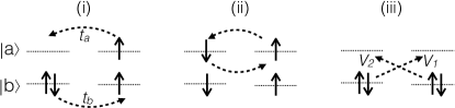
Figure 8: Nearest-neighbor hopping processes in undoped system with marked amplitudes $t_{a}$ and $t_{b}$ and cross-hopping ${V_{1}=\pm V_{2}}$: (i) hopping of HS boson, (ii) super-exchange between HS states, (iii) pair creation/annihilation due to cross-hopping.

Undoped case. The ground state of the undoped system is determined by the second-order processes in hopping. Kuneš (2015) In Fig. 8 we summarize the most important of these processes. The numerical results can be understood by looking at the signs of the different contributions to the variational energy $\langle CC|H|CC\rangle$ on the nearest-neighbor bonds

$$\begin{split}\langle C_{i}C_{j}|H^{(i)}|C_{i}C_{j}\rangle&\sim t_{a}t_{b}s^{2}\operatorname{Re}({\xi_{1}^{(j)}}^{*}\xi_{1}^{(i)}+{\xi_{-1}^{(j)}}^{*}\xi_{-1}^{(i)})\\ \langle C_{i}C_{j}|H^{(ii)}|C_{i}C_{j}\rangle&\sim-(t_{a}^{2}+t_{b}^{2})\left(|\xi_{1}^{(i)}|^{2}|\xi_{-1}^{(j)}|^{2}+|\xi_{-1}^{(i)}|^{2}|\xi_{1}^{(j)}|^{2}\right)\\ \langle C_{i}C_{j}|H^{(iii)}|C_{i}C_{j}\rangle&\sim-V_{1}V_{2}s^{2}\operatorname{Re}\left(\xi_{1}^{(j)}\xi_{-1}^{(i)}+\xi_{-1}^{(j)}\xi_{1}^{(i)}\right).\end{split}$$

The term $H^{(i)}$, which drives the transition and selects the uniform order for $t_{a}t_{b}<0$, does not distinguish between the excitonic phases. The term $H^{(ii)}$, arising from nearest-neighbor anti-ferromagnetic exchange, favors the PEC phase with $|\xi_{1}|=|\xi_{-1}|$. The processes discussed so far do not distinguish the phase of the complex order parameter. The pair-creation term $H^{(iii)}$ does. However, for real $V_{1,2}$ it is sensitive only to the total phase of $\xi_{1}\xi_{-1}$ and depending on the sign of $V_{1}V_{2}$ it selects its value to be either 0 or $\pi$. Both of these states can be realized with purely real $\xi_{1}=\xi_{-1}$ or $\xi_{1}=-\xi_{-1}$. Using real $\xi_{1,-1}$ therefore amounts, at least on the level of product state (5), to selecting a specific direction of $\bm{\xi}$ (which will be shown to translate to the direction of spin polarization) among the possible degenerate choices. For even cross-hopping $V_{1}=V_{2}$, $H^{(iii)}$ selects the SCDW state $\xi_{1}=\xi_{-1}$ ($\phi_{+}=-\phi_{-}$), while for the odd cross-hopping $V_{1}=-V_{2}$ it selects the SDW state $\xi_{1}=-\xi_{-1}$ ($\phi_{+}=\phi_{-}$).

Doped case. When doped the low-energy Hilbert space contains additional states $|\uparrow\rangle$ and $|\downarrow\rangle$ that give rise to additional exchange process between the bosonic and fermionic excitations shown in Figs. 9,10. The simplest way to account for these processes in the low doping regime is to compute the matrix elements describing the propagation of the doped carriers on the condensate background. This approach is well known from the treatment of double-exchange interaction and was recently applied in a context similar to our model. Chaloupka and Khaliullin (2016) For the sake of completeness we evaluate the matrix elements for general $\bm{\xi}$. The contribution from hopping within the $b$-band (iv) reads

$$\langle\sigma_{i}C_{j}|H^{(iv)}|C_{i}\sigma_{j}\rangle=-t_{b}s^{2}.$$ (8)

The contribution from hopping within the $a$-band (v) is spin-dependent and reads

$$\begin{split}\langle\uparrow_{i}C_{j}|H^{(v)}|C_{i}\uparrow_{j}\rangle&=-t_{a}\left({\xi_{1}^{(j)}}^{*}\xi_{1}^{(i)}+\frac{1}{2}{\xi_{0}^{(j)}}^{*}\xi_{0}^{(i)}\right)\\ \langle\downarrow_{i}C_{j}|H^{(v)}|C_{i}\downarrow_{j}\rangle&=-t_{a}\left({\xi_{-1}^{(j)}}^{*}\xi_{-1}^{(i)}+\frac{1}{2}{\xi_{0}^{(j)}}^{*}\xi_{0}^{(i)}\right)\\ \langle\uparrow_{i}C_{j}|H^{(v)}|C_{i}\downarrow_{j}\rangle&=-\frac{t_{a}}{\sqrt{2}}\left({\xi_{-1}^{(j)}}^{*}\xi_{0}^{(i)}+{\xi_{0}^{(j)}}^{*}\xi_{1}^{(i)}\right)\\ \langle\downarrow_{i}C_{j}|H^{(v)}|C_{i}\uparrow_{j}\rangle&=-\frac{t_{a}}{\sqrt{2}}\left({\xi_{1}^{(j)}}^{*}\xi_{0}^{(i)}+{\xi_{0}^{(j)}}^{*}\xi_{-1}^{(i)}\right).\end{split}$$ (9)

The cross-hopping processes, Fig. 10, give rise to

$$\begin{split}\langle\uparrow_{i}C_{j}|H^{(vi)}|C_{i}\uparrow_{j}\rangle&=\frac{V_{1}^{(ji)}}{\sqrt{2}}s{\xi_{0}^{(j)}}^{*}\\ \langle\downarrow_{i}C_{j}|H^{(vi)}|C_{i}\downarrow_{j}\rangle&=-\langle\uparrow C|H^{(vi)}|C\uparrow\rangle\\ \langle\uparrow_{i}C_{j}|H^{(vi)}|C_{i}\downarrow_{j}\rangle&=V_{1}^{(ji)}s{\xi_{-1}^{(j)}}^{*}\\ \langle\downarrow_{i}C_{j}|H^{(vi)}|C_{i}\uparrow_{j}\rangle&=-V_{1}^{(ji)}Ts{\xi_{1}^{(j)}}^{*}\end{split}$$ (10)

and

$$\begin{split}\langle\uparrow_{i}C_{j}|H^{(vii)}|C_{i}\uparrow_{j}\rangle&=\frac{V_{2}^{(ji)}}{\sqrt{2}}s\xi_{0}^{(i)}\\ \langle\downarrow_{i}C_{j}|H^{(vii)}|C_{i}\downarrow_{j}\rangle&=-\langle\uparrow C|H^{(vi)}|C\uparrow\rangle\\ \langle\uparrow_{i}C_{j}|H^{(vii)}|C_{i}\downarrow_{j}\rangle&=-V_{2}^{(ji)}s\xi_{1}^{(i)}\\ \langle\downarrow_{i}C_{j}|H^{(vii)}|C_{i}\uparrow_{j}\rangle&=V_{2}^{(ji)}s\xi_{-1}^{(i)}.\end{split}$$ (11)

The dynamics of the doped hole is thus described by an effective single-band Hamiltonian

$$\begin{split}H_{\text{eff}}=\sum_{ij}h^{(ij)}_{\alpha\beta}\tilde{b}^{\dagger}_{i\alpha}\tilde{b}^{\phantom{\dagger}}_{j\beta},\\ \text{with}\ \ h_{\alpha\beta}^{(ij)}=\langle\alpha_{i}C_{j}|H|C_{i}\beta_{j}\rangle\end{split}$$ (12)

being the effective hopping on bond $ij$. Using Cartesian representation (6) the effective hopping can be expressed in a compact form

$$\begin{split}\bar{h}^{(ij)}=&-\left(t_{b}s^{2}+t_{a}\left(1-s^{2}\right)\right)\bar{I}\\ &+\frac{t_{a}}{4}i\left({\bm{\xi}^{(j)}}^{*}\wedge\bm{\xi}^{(i)}\right)\cdot\bar{\bm{\sigma}}\\ &+\frac{1}{2}\left(V_{1}^{(ji)}s{\bm{\xi}^{(j)}}^{*}+V_{2}^{(ji)}s\bm{\xi}^{(i)}\right)\cdot\bar{\bm{\sigma}},\end{split}$$ (13)

where the bar denotes $2\times 2$ matrices. For density-density interaction, which imposes the constraint $\xi_{0}=0$ the above equation reduces to

$$\bar{h}^{(ij)}=\begin{pmatrix}-t_{b}s^{2}-t_{a}{\xi_{1}^{(j)}}^{*}\xi_{1}^{(i)}&V_{1}^{(ji)}s{\xi_{-1}^{(j)}}^{*}-V_{2}^{(ji)}s\xi_{1}^{(i)}\\ -V_{1}^{(ji)}s{\xi_{1}^{(j)}}^{*}+V_{2}^{(ji)}s\xi_{-1}^{(i)}&-t_{b}s^{2}-t_{a}{\xi_{-1}^{(j)}}^{*}\xi_{-1}^{(i)}\end{pmatrix}$$ (14)

Hamiltonian $H_{\text{eff}}$ contains the usual spin-preserving hopping and two ’magnetic’ terms proportional to $\xi$ and $\xi^{2}$. The ’magnetic’ terms correspond to spin-dependent hopping that can be viewed as ’magnetic’ fields acting on the bonds, which give rise to ’magnetic’ fields acting locally in reciprocal space. With $i\bm{\xi}^{*}\wedge\bm{\xi}$ being the magnetic polarization of the condensate Balents (2000); Kuneš (2015) the $\xi^{2}$-term is analogous to the Zener double-exchange interaction. Zener (1951) The magnetic polarization is perpendicular to the order parameter and is not sensitive to the phase of $\bm{\xi}$.

The $\xi$-linear term appears only for non-zero cross hopping. It gives rise to a polarization parallel to $\bm{\xi}$. Similar to the undoped case we can show that the mean-field ground-state energy can be minimized with real $\xi_{1,2}$. The kinetic energy of the doped carriers (eigenvalues of $H_{\text{eff}}(\mathbf{k})$) depends only on the amplitude of the off-diagonal elements of $H_{\text{eff}}$. This is, for $\xi_{0}=0$, proportional to $V^{2}_{1}|\xi_{-1}|^{2}+V^{2}_{2}|\xi_{1}|^{2}-2V_{1}V_{2}\operatorname{Re}(\xi_{1}\xi_{-1})$.

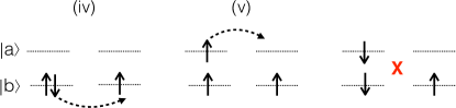
Figure 9: Nearest-neighbor processes allowing the propagation of dopes holes in system without cross-hopping: (iv) spin-independent hole propagation, (v) spin-dependent hole propagation.

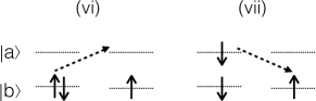
Figure 10: Additional spin-flip hopping of doped holes due to cross-hopping.

I.3 Spin-density distribution

In the following we give an explicit formula for real space spin density $\mathbf{m}(\mathbf{r})$ as a function of the $\mathbf{k}$-dependent one-particle density matrix. As in the main text, we assume that the corresponding orbitals are real functions $\varphi_{\alpha}(\mathbf{r})$. The summation over the spin indices $\sigma$, $\sigma^{\prime}$ is implied.

$$\begin{split}\mathbf{m}(\mathbf{r})&=\bm{\tau}_{\sigma\sigma^{\prime}}\langle\psi^{\dagger}_{\sigma}(\mathbf{r})\psi_{\sigma^{\prime}}(\mathbf{r})\rangle\\ &=\sum_{\mathbf{R},\mathbf{R}^{\prime}}\sum_{\alpha,\beta}\varphi_{\alpha}(\mathbf{r}-\mathbf{R})\varphi_{\beta}(\mathbf{r}-\mathbf{R}^{\prime})\bm{\tau}_{\sigma\sigma^{\prime}}\langle c_{\alpha\sigma}^{\dagger}(\mathbf{R})c_{\beta\sigma^{\prime}}^{\phantom{\dagger}}(\mathbf{R}^{\prime})\rangle\\ &=\sum_{\mathbf{R},\mathbf{R}^{\prime}}\sum_{\alpha}\varphi_{\alpha}(\mathbf{r}-\mathbf{R})\varphi_{\alpha}(\mathbf{r}-\mathbf{R}^{\prime})\sum_{\mathbf{k}}\cos\mathbf{k}(\mathbf{R}-\mathbf{R}^{\prime})\bm{\tau}_{\sigma\sigma^{\prime}}\langle c_{\alpha\sigma}^{\dagger}(\mathbf{k})c_{\alpha\sigma^{\prime}}^{\phantom{\dagger}}(\mathbf{k})\rangle\\ &+\sum_{\mathbf{R},\mathbf{R}^{\prime}}\sum_{\alpha>\beta}\varphi_{\alpha}(\mathbf{r}-\mathbf{R})\varphi_{\beta}(\mathbf{r}-\mathbf{R}^{\prime})\sum_{\mathbf{k}}e^{-i\mathbf{k}\cdot(\mathbf{R}-\mathbf{R}^{\prime})}\bm{\tau}_{\sigma\sigma^{\prime}}\langle c_{\alpha\sigma}^{\dagger}(\mathbf{k})c_{\beta\sigma^{\prime}}^{\phantom{\dagger}}(\mathbf{k})+c_{\beta\sigma}^{\dagger}(-\mathbf{k})c_{\alpha\sigma^{\prime}}^{\phantom{\dagger}}(-\mathbf{k})\rangle\end{split}$$ (15)

References

Dresselhaus (1955)
G. Dresselhaus,
Phys. Rev. 100,
580 (1955).
Rashba (1960)
E. Rashba,
Sov. Phys. Solid State 2,
1109 (1960).
Manchon et al. (2015)
A. Manchon,
H. C. Koo,
J. Nitta,
S. M. Frolov,
and R. A. Duine,
Nature Mater. 14,
871 (2015).
Manchon and Zhang (2008)
A. Manchon and
S. Zhang,
Phys. Rev. B 78,
212405 (2008).
Li et al. (2015)
H. Li,
H. Gao,
L. P. Zârbo,
K. Výborný,
X. Wang,
I. Garate,
F. Doǧan,
A. Čejchan, J. Sinova,
T. Jungwirth,
et al., Phys. Rev. B
91, 134402
(2015).
Železný
et al. (2014)
J. Železný, H. Gao,
K. Výborný,
J. Zemen,
J. Mašek, A. Manchon,
J. Wunderlich,
J. Sinova, and
T. Jungwirth,
Phys. Rev. Lett. 113,
157201 (2014).
Wadley et al. (2016)
P. Wadley,
B. Howells,
J. Železný,
C. Andrews,
V. Hills,
R. P. Campion,
V. Novák,
K. Olejník,
F. Maccherozzi,
S. S. Dhesi,
et al., Science
351,
587 (2016).
Wunderlich et al. (2009)
J. Wunderlich,
A. C. Irvine,
J. Sinova,
B. G. Park,
L. P. Zârbo,
X. L. Xu,
B. Kaestner,
V. Novák, and
T. Jungwirth,
Nature Phys. 5,
675 (2009).
Nagaosa et al. (2012)
N. Nagaosa,
X. Z. Yu, and
Y. Tokura,
Phil. Trans. R. Soc. 370,
5806 (2012).
Jonietz et al. (2010)
F. Jonietz,
S. Mühlbauer,
C. Pfleiderer,
A. Neubauer,
W. Münzer,
A. Bauer,
T. Adams,
R. Georgii,
P. Böni,
R. A. Duine,
et al., Science
330, 1648 (2010).
Wu and Zhang (2004)
C. Wu and
S.-C. Zhang,
Phys. Rev. Lett. 93,
036403 (2004).
Vollhardt and Wölfle (2013)
D. Vollhardt and
P. Wölfle,
The Superfluid Phases of Helium 3
(Dover, New Yourk,
2013), reprint ed.
Wu et al. (2007)
C. Wu,
K. Sun,
E. Fradkin, and
S.-C. Zhang,
Phys. Rev. B 75,
115103 (2007).
Khaliullin (2013)
G. Khaliullin,
Phys. Rev. Lett. 111,
197201 (2013).
Kuneš and
Augustinský (2014a)
J. Kuneš and
P. Augustinský,
Phys. Rev. B 89,
115134 (2014a).
Halperin and Rice (1968)
B. I. Halperin and
T. M. Rice,
Solid State Physics (Academic
Press, New York, 1968),
vol. 21, p. 115.
Balents (2000)
L. Balents,
Phys. Rev. B 62,
2346 (2000).
Kuneš (2015)
J. Kuneš,
J. Phys.: Condens. Matter 27,
333201 (2015).
Kuneš and
Augustinský (2014b)
J. Kuneš and
P. Augustinský,
Phys. Rev. B 90,
235112 (2014b).
Cao et al. (2014)
G. Cao,
T. F. Qi,
L. Li,
J. Terzic,
S. J. Yuan,
L. E. DeLong,
G. Murthy, and
R. K. Kaul,
Phys. Rev. Lett. 112,
056402 (2014).
(21)
A. Jain,
M. Krautloher,
J. Porras,
G. H. Ryu,
D. P. Chen,
D. L. Abernathy,
J. T. Park,
A. Ivanov,
J. Chaloupka,
G. Khaliullin,
et al., arXiv:1510.07011.
Dey et al. (2016)
T. Dey,
A. Maljuk,
D. V. Efremov,
O. Kataeva,
S. Gass,
C. G. F. Blum,
F. Steckel,
D. Gruner,
T. Ritschel,
A. U. B. Wolter,
et al., Phys. Rev. B
93, 014434
(2016).
Pajskr et al. (2016)
K. Pajskr,
P. Novák,
V. Pokorný,
J. Kolorenč, R. Arita,
and
J. Kuneš, Phys. Rev. B 93,
035129 (2016).
Kuneš (2014)
J. Kuneš, Phys. Rev. B 90,
235140 (2014).
Kaneko and Ohta (2014)
T. Kaneko and
Y. Ohta,
Phys. Rev. B 90,
245144 (2014).
Kaneko et al. (2015)
T. Kaneko,
B. Zenker,
H. Fehske, and
Y. Ohta,
Phys. Rev. B 92,
115106 (2015).
(27)
S. Hoshino and
P. Werner,
Phys. Rev. B 93,
155161 (2016).
Chaloupka and Khaliullin (2016)
J. Chaloupka and
G. Khaliullin,
Phys. Rev. Lett. 116,
017203 (2016).
Zener (1951)
C. Zener,
Phys. Rev. 82,
403 (1951).
Werner et al. (2006)
P. Werner,
A. Comanac,
L. de’ Medici,
M. Troyer, and
A. J. Millis,
Phys. Rev. Lett. 97,
076405 (2006).
Albuquerque et al. (2007)
A. Albuquerque,
F. Alet,
P. Corboz,
P. Dayal,
A. Feiguin,
S. Fuchs,
L. Gamper,
E. Gull,
S. Gürtler,
A. Honecker,
et al., Journal of Magnetism and Magnetic
Materials 310, 1187
(2007), ISSN 0304-8853,
proceedings of the 17th International Conference on
MagnetismThe International Conference on Magnetism.
Gubernatis et al. (1991)
J. E. Gubernatis,
M. Jarrell,
R. N. Silver,
and D. S. Sivia,
Phys. Rev. B 44,
6011 (1991).