Direct extraction of nuclear effects in quasielastic scattering on carbon

Abstract

Nuclear effects on neutrino reactions are expected to be a significant complication in current and future neutrino oscillation experiments seeking precision measurements of neutrino flavor transitions. Calculations of these nuclear effects are hampered by a lack of experimental data comparing neutrino reactions on free nucleons to neutrino reactions on nuclei. We present results from a novel technique that compares neutrino and antineutrino charged current quasielastic scattering on hydrocarbons to extract a cross section ratio of antineutrino charged current elastic reactions on free protons to charged current quasielastic reactions on the protons bound in a carbon nucleus. This measurement of nuclear effects is compared to models.

The cross sections for neutrino and antineutrino charged current quasielastic (CCQE) reactions on free nucleons, $\nu_{\ell}n\to\ell^{-}p$ and $\bar{\nu}_{\ell}p\to\ell^{+}n$, can be expressed in terms of nucleon form factors Adler (1963); Marshak et al. (1969); Pais (1971); Llewellyn Smith (1972). This prescription, with form factors constrained by electron nucleon elastic scattering and pion electroproduction data, accurately describes available neutrino interaction data on hydrogen and loosely bound deuterium targets Budd et al. (2003); Kuzmin et al. (2006); Bodek et al. ; Kuzmin et al. (2008); Bodek et al. (2008). On heavier, more tightly bound nuclei, the relativistic Fermi Gas (FG) model Smith and Moniz (1972) modifies this formalism within the context of the impulse approximation to include a simple description of the initial state of bound nucleons within the nucleus, and has been extensively used in neutrino interaction generators. However, experiments with carbon, oxygen and iron targets Aguilar-Arevalo et al. (2010); Gran et al. (2006); Lyubushkin et al. (2009); Dorman (2009); Fiorentini et al. (2013); Fields et al. (2013); Aguilar-Arevalo et al. (2013); Abe et al. (2015a, b) with neutrino energies of a few GeV have measured a significantly different, typically higher, quasielastic cross section than predicted by the FG model. Additionally, recent measurements of the CC-inclusive cross section have shown that nuclear effects are not well understood Rodrigues et al. (2016), and that the ratio of CC-inclusive cross section measurements on different nuclear targets cannot be described by the models available in generators Tice et al. (2014), particularly in the elastic region.

Theoretical work to understand these differences have been focused on three broad areas: a more sophisticated description of the initial state of nucleons within the nucleus Benhar and Fabrocini (2000); Ankowski and Sobczyk (2006); Butkevich (2009); Bodek et al. (2014); Leitner et al. (2009); Maieron et al. (2003); Meucci et al. (2004); Pandey et al. (2015); contributions to the cross section beyond the impulse approximation which involve multiple initial state nucleons (hereafter referred to as multinucleon processes or MNP) Nieves et al. (2011); Martini et al. (2009); and collective effects which modify the cross section, which are generally referred to by the name of the calculation, the Random Phase Approximation (RPA) Nieves et al. (2011); Martini et al. (2009). Despite the flurry of theoretical activity in recent years, a consistent picture has yet to emerge, in part because of significant differences in the predictions of theoretical calculations Formaggio and Zeller (2012); Alvarez-Ruso et al. (2014); Garvey et al. (2015).

Quasielastic interactions are especially important for accelerator neutrino oscillation experiments at GeV energies Aguilar-Arevalo et al. (2009a); Abe et al. (2011a); Ayres et al. (2005); Abe et al. (2011b); Acciarri et al. (2016). In the impulse approximation, the initial state nucleons are independent in the mean field of the nucleus, and therefore the neutrino energy and momentum transfer $Q^{2}$ can be estimated from the polar angle $\theta_{\ell}$ and momentum $p_{\ell}$ of the final state lepton. However, the initial state prescription and multinucleon processes both disrupt this relationship in different ways Martini et al. (2013); Lalakulich and Mosel (2012); Nieves et al. (2012). MNP and collective RPA processes both alter the distribution of $Q^{2}$ which can in turn alter the relative acceptance of near and far detectors. Therefore understanding nuclear modifications is essential for the current and future generations of neutrino oscillation experiments.

Although neutrino–nucleon scattering data would be invaluable for untangling nuclear effects, no new data are expected from any current or planned experiments in the few-GeV energy region. In this analysis, we present a method for extracting a measurement of the suppression and enhancement to the CCQE cross section due to nuclear effects in carbon from neutrino and antineutrino measurements on hydrocarbon targets, which is relatively free of axial form factor and other uncertainties, particularly at low $Q^{2}$. This method is largely model independent when applied to high energy CCQE data, such as that from MINER$\nu$A Fiorentini et al. (2013); Fields et al. (2013), but less so at the lower energies of the MiniBooNE experiment Aguilar-Arevalo et al. (2010, 2013).

The CCQE neutrino–nucleon differential cross section for free nucleons as a function of the negative of the four-momentum transfer squared, $Q^{2}$, can be expressed using the Llewellyn-Smith formula Llewellyn Smith (1972):

$$\frac{d\sigma}{dQ^{2}} {\nu_{l}n\rightarrow l^{-}p\choose\bar{\nu}_{l}p\rightarrow l^{+}n}=\frac{M^{2}G_{\mathrm{F}}^{2}\cos^{2}\vartheta_{C}}{8\pi E_{\nu}^{2}}$$

$$\times\left[A(Q^{2})\pm B^{\prime}(Q^{2})\frac{(s-u)}{M^{4}}+C(Q^{2})\frac{(s-u)^{2}}{M^{4}}\right],$$ (1)

where $M$ is the mass of the struck nucleon, $G_{\mathrm{F}}$ is Fermi’s constant, $\vartheta_{C}$ is the Cabibbo angle, $E_{\nu}$ is the incoming neutrino energy and $s$ and $u$ are the Mandelstam variables. $A(Q^{2})$, $B^{\prime}(Q^{2})$ and $C(Q^{2})$ are functions of the vector form factors: $F_{\mathrm{V}}^{1,\;2}$, constrained by electron nucleon elastic scattering experiments Budd et al. (2003); Bodek et al. ; the axial form factor, $F_{\mathrm{A}}$, constrained by neutrino scattering experiments on hydrogen and deuterium and from pion electroproduction Kuzmin et al. (2006); Bodek et al. ; Kuzmin et al. (2008); Bodek et al. (2008); and the pseudoscalar form factor, $F_{\mathrm{P}}$, which is derived from $F_{\mathrm{A}}$ Llewellyn Smith (1972). Uncertainties from $F_{\mathrm{P}}$ and the assumption that second class currents can be neglected are discussed in Reference Day and McFarland (2012). The term with $B^{\prime}(Q^{2})$ contains the interference between the axial and vector currents, and it is this term which is responsible for the $Q^{2}$ dependent difference between the $\nu_{\ell}+n\rightarrow\ell^{-}+p$ and $\bar{\nu}_{\ell}+p\rightarrow\ell^{+}+n$ cross sections. At $Q^{2}=0$, there is no difference between the CCQE cross sections for neutrinos and antineutrinos. Note that $s-u=4ME_{\nu}-Q^{2}-m_{\ell}^{2}$, where $m_{\ell}$ is the mass of the final state lepton; therefore, the effect of the interference term is largest at small neutrino energies and high $Q^{2}$.

Nuclear models available in the NEUT Hayato (2009); Wilkinson et al. (2016) event generator will be compared to the data. NEUT’s default model is the Smith-Moniz Smith and Moniz (1972) implementation of an FG model with Fermi momentum ($p_{\mathrm{F}}$) and binding energy ($E_{\mathrm{b}}$) on carbon set to $p_{\mathrm{F}}$ = 217 MeV and $E_{\mathrm{b}}$ = 25 MeV based on electron scattering data Moniz et al. (1971). NEUT has implemented the Spectral Function (SF) model of Benhar Benhar and Fabrocini (2000); Furmanski (2015) which describes the initial nucleon’s correlated momentum and removal energy and includes short range nuclear correlations which affect $\sim$20% of the CCQE rate. Nuclear screening due to long-range nucleon correlations is implemented in RPA calculations Nieves et al. (2011). Calculations of MNP use the model of Nieves et al. Nieves et al. (2011); Gran et al. (2013). NEUT also has implementations of two effective models constructed to ensure agreement with electron data, an Effective Spectral Function (ESF) Bodek et al. (2014, 2015); Wilkinson (2015) and the Transverse Enhancement Model (TEM) Bodek et al. (2011); Wilkinson (2015). For all models, we use the BBBA05 vector nucleon form factors Bradford et al. (2006) and a dipole axial form factor with $M_{\textrm{A}}$ = 1.00 GeV, based on fits to bubble chamber data Kuzmin et al. (2006); Bodek et al. ; Kuzmin et al. (2008); Bodek et al. (2008).

In this analysis we use the published flux-averaged neutrino and antineutrino CCQE cross section results on hydrocarbon targets from the MINER$\nu$A Fiorentini et al. (2013); Fields et al. (2013) and MiniBooNE Aguilar-Arevalo et al. (2010, 2013) experiments. The results used are differential in terms of $Q^{2}_{\textrm{QE}}$, derived from lepton kinematics under the quasielastic hypothesis,

$$Q^{2}_{\textrm{QE}}=-m_{\mu}^{2}+2E_{\nu}^{\mbox{\scriptsize{QE,\;FG}}}(E_{\mu}-\sqrt{E_{\mu}^{2}-m_{\mu}^{2}}\cos{\theta_{\mu}}),$$

$$E_{\nu}^{\mbox{\scriptsize{QE,\;FG}}}=\frac{2M^{\prime}_{i}E_{\mu}-(M^{\prime 2}_{i}+m_{\mu}^{2}-M^{2}_{f})}{2(M^{\prime}_{i}-E_{\mu}+\sqrt{E_{\mu}^{2}-m_{\mu}^{2}}\cos{\theta_{\mu}})},$$ (2)

where $E_{\mu}$ is the muon energy, $m_{\mu}$ is the muon mass, $M_{i}$ ($M_{f}$) is the initial (final) nucleon mass, and $M^{\prime}_{i}=M_{i}-V$ where $V$ is the effective binding energy. For both MiniBooNE datasets and for the MINER$\nu$A neutrino dataset, $V=34$ MeV; for the MINER$\nu$A antineutrino dataset, $V=30$ MeV.

There are three differences in the neutrino and antineutrino cross section measurements for CCQE-like processes on hydrocarbon, $CH_{\mathrm{N}}$ targets. Firstly, the neutrino and antineutrino cross sections are fundamentally different for free nucleons (see Equation 1). Secondly, the neutrino and antineutrino fluxes produced in the same beamline may be different Kopp (2005); Aguilar-Arevalo et al. (2009b). Finally, antineutrinos can interact with the free proton from the hydrogen as well as bound protons within the carbon nucleus, whereas neutrinos can only interact with bound neutrons. The central thesis of this work is that a direct measurement of nuclear effects in carbon can be made by

$$\frac{6\sigma^{\bar{\nu}}_{\mathrm{H}}}{\sigma_{\mathrm{C}}^{\bar{\nu}}}=\frac{\left[(6+N)\widetilde{\sigma}^{\bar{\nu}}_{\mathrm{CH_{N}}}-6\lambda(Q^{2})\widetilde{\sigma}^{\nu}_{\mathrm{CH_{N}}}\right]}{N\lambda(Q^{2})\widetilde{\sigma}^{\nu}_{\mathrm{CH_{N}}}},$$ (3)

where $\sigma$ denotes the flux-averaged cross section for interactions between the neutrino species in the superscript and the the target in the subscript; $\widetilde{\sigma}$ denotes a cross section per nucleon; the correction factor $\lambda(Q^{2})=(d\sigma^{\bar{\nu}}_{p}/dQ^{2})/(d\sigma^{\nu}_{n}/dQ^{2})$ corrects for the difference between the neutrino and antineutrino nucleon cross sections and fluxes and is shown in Figure 1.

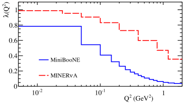
Figure 1: $\lambda(Q^{2})=\sigma^{\bar{\nu}}_{p}(Q^{2})/\sigma^{\nu}_{n}(Q^{2})$ calculated using the free nucleon cross-sections implemented in the GENIE neutrino interaction generator Andreopoulos et al. (2010), averaged over the relevant flux and binned into the $Q^{2}$ binning used by the relevant experiment. The values are given in Appendix III.

The validity of Equation 3 rests on the assumption that the ratio of bound to free cross sections, as a function of $Q^{2}$, is the same for neutrino and antineutrino scattering. The quality of this assumption can be tested directly for a variety of models by looking at the double ratio $R(Q^{2})$,

$$R(Q^{2})=\left.\left(\frac{6\sigma^{\bar{\nu}}_{p}(Q^{2})}{\sigma^{\bar{\nu}}_{C}(Q^{2})}\right)\middle/\left(\frac{6\sigma^{\nu}_{n}(Q^{2})}{\sigma^{\nu}_{C}(Q^{2})}\right)\right.,$$ (4)

where the bound CCQE cross section for neutrino and antineutrino ($\sigma^{\bar{\nu}}_{C}(Q^{2})$ and $\sigma^{\nu}_{C}(Q^{2})$) is calculated for any given nuclear model. Deviations of $R$ from 1 indicate that this assumption is inadequate and will lead to biases in results extracted with Equation 3. Within an FG model, the assumption that $R=1$ is imperfect due to the effects of binding energy and kinematic boundaries, and this point is discussed further in Appendix I. The bias to our extracted results can be seen in the generalization of Equation 3 for the case where $R\neq 1$:

$$\frac{6\sigma^{\bar{\nu}}_{\mathrm{H}}}{\sigma_{\mathrm{C}}^{\bar{\nu}}} = \frac{\left[(6+N)\widetilde{\sigma}^{\bar{\nu}}_{\mathrm{CH_{N}}}-6\lambda(Q^{2})\widetilde{\sigma}^{\nu}_{\mathrm{CH_{N}}}\right]}{N\lambda(Q^{2})\widetilde{\sigma}^{\nu}_{\mathrm{CH_{N}}}},$$ (5)

$$+\left[\frac{6+N}{N\lambda(Q^{2})}\frac{\widetilde{\sigma}^{\bar{\nu}}_{\mathrm{CH_{N}}}}{\widetilde{\sigma}^{\nu}_{\mathrm{CH_{N}}}}(R-1)\right]\rightarrow\mathrm{{\it R}-term}.$$

We determine the size of the $R$-term MINER$\nu$A and MiniBooNE fluxes for the nuclear models discussed above in Figure 2. The $R$-term is relatively flat across the entire $Q^{2}$ range for MINER$\nu$A, with no indication of strong biases, which suggests that our assumption holds well in this case and our results will be unbiased and do not depend strongly on the choice of nuclear model. For MiniBooNE, the assumption does not hold up as well, so we expect biases in results extracted using Equation 3.

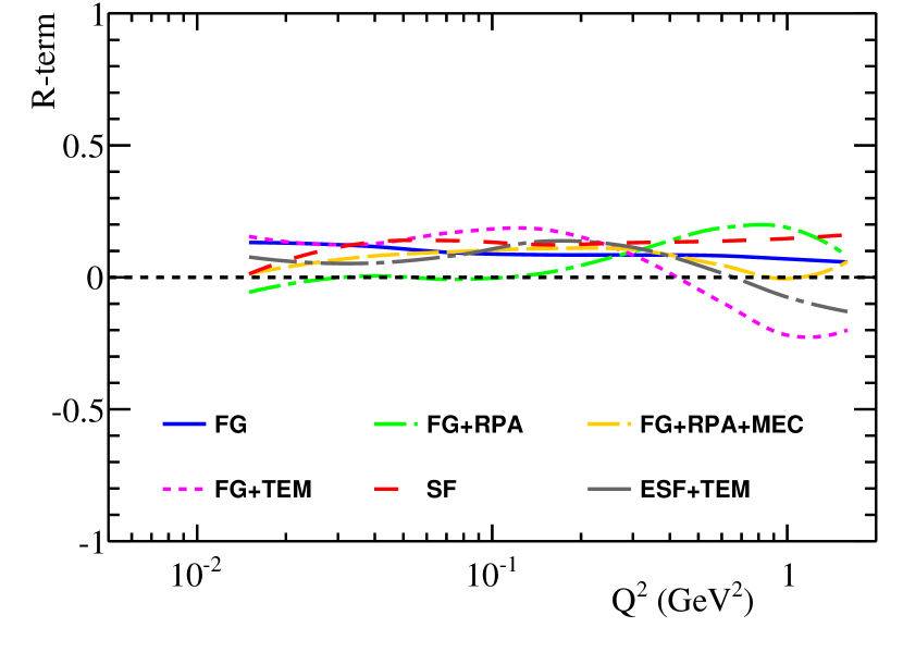
(a) MINER$\nu$A

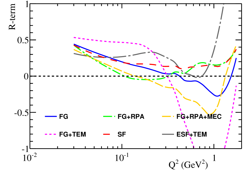
(b) MiniBooNE

Figure 2: The $R$-term, defined in Equation 5, is shown for both MINER$\nu$A and MiniBooNE, for a variety of models. It shows the size of the bias on the value $\frac{6\sigma^{\bar{\nu}}_{\mathrm{H}}}{\sigma_{\mathrm{C}}^{\bar{\nu}}}$, extracted using Equation 3, which is due to our assumption that the neutrino and antineutrino cross section ratio is the same for free nucleons and bound nucleons. A value of 0 indicates no bias. The statistical error from the MC is $\sim$0.05 for all bins and is uncorrelated between all bins and models.

Another complication of this analysis is that experiments measure differential cross-sections in $Q^{2}_{\textrm{QE}}$, as defined in Equation 2, whereas the technique relates differential cross sections in $Q^{2}$. Appendix II shows the relationship between these two in the FG model. The differences are small compared to $Q^{2}$ bin widths for all relevant kinematics in the MINER$\nu$A experiment; however, in MiniBooNE, the smearing becomes comparable to the bin width for $Q^{2}>0.2$ GeV².

The measurement of nuclear effects on carbon is extracted from the public data releases for MINER$\nu$A Fiorentini et al. (2013); Fields et al. (2013) and MiniBooNE Aguilar-Arevalo et al. (2010, 2013) using Equation 3 with standard propagation of error techniques. For MINER$\nu$A, the full covariance matrix, including cross-correlations, of the neutrino and antineutrino datasets is provided. For MiniBooNE, only the diagonals from the shape covariance matrices, and overall normalization factors are provided separately for the neutrino and antineutrino datasets (which we assume to to be uncorrelated in this analysis). The data points and covariance matrices extracted in this work for both MINER$\nu$A and MiniBooNE are available in the supplementary material.

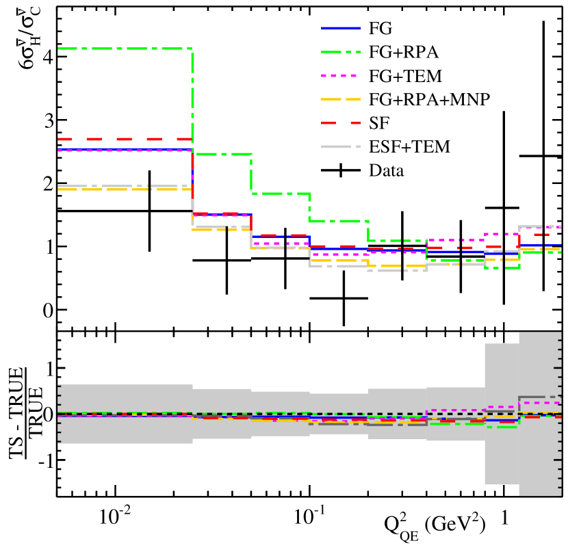
(a) MINER$\nu$A

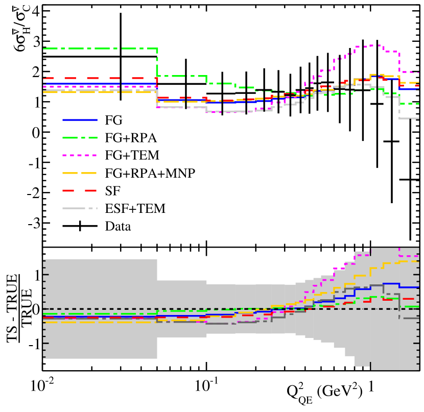
(b) MiniBooNE

Figure 3: The value of $6\sigma^{\bar{\nu}}_{\mathrm{H}}/\sigma_{\mathrm{C}}^{\bar{\nu}}$ calculated using Equation 3 is shown for a variety of NEUT models, as well as for the extracted MINER$\nu$A and MiniBooNE data. The model dependent bias on $6\sigma^{\bar{\nu}}_{\mathrm{H}}/\sigma_{\mathrm{C}}^{\bar{\nu}}$ is quantified by comparing the value obtained with Equation 3 (TS) with the exact value calculated for each model (TRUE). The bias, $\frac{\mathrm{TS}-\mathrm{TRUE}}{\mathrm{TRUE}}$, is compared with the fractional uncertainty on the measurement from data.

In Figure 3, the test statistic of Equation 3 is calculated for the MINER$\nu$A and MiniBooNE data, and compared with the nuclear enhancement or suppression predicted by a variety of CCQE cross section models available in NEUT. The power of our measurement to constrain the choice of nuclear model is shown by the difference between our extracted data points and the ratio predicted by the various models tested. A $\chi^{2}$ value can be calculated for each model

$$\chi^{2}=\left(\nu_{i}^{\mbox{\scriptsize{DATA}}}-\nu_{i}^{\mbox{\scriptsize{MC}}}\right)M^{-1}_{ij}\left(\nu_{j}^{\mbox{\scriptsize{DATA}}}-\nu_{j}^{\mbox{\scriptsize{MC}}}\right),$$ (6)

where the measurement of nuclear effects from data is given by $\nu_{i}^{\mbox{\scriptsize{DATA}}}$, the covariance matrix between the data points is $M_{ij}$ and the NEUT prediction for each model is given with $\nu_{i}^{\mbox{\scriptsize{MC}}}$. The $\chi^{2}$ values for each model are given for both MINER$\nu$A and MiniBooNE in Table 1. The models to which we compare the data span calculational approaches to nuclear models for CCQE in the literature, but are not a complete set. Any other model can be compared to the measurements in this work using information in Appendix III.

Model	$\chi^{2}$/DOF
	MINER$\nu$A	MiniBooNE
FG	14.8/8	6.0/17
FG+RPA	44.3/8	6.0/17
FG+RPA+MNP	13.6/8	6.8/17
FG+TEM	13.4/8	23.4/17
SF	15.9/8	6.1/17
ESF+TEM	12.8/8	6.2/17

Table 1: $\chi^{2}$ values obtained with Equation 6 for the various cross section models shown in Figure 3.

Any model dependent bias in the test statistic due to the free nucleon correction factor $\lambda(Q^{2})$ (see Equation 5 and Figure 2) or $Q^{2}\rightarrow Q^{2}_{\textrm{QE}}$ differences (see Appendix II) can be calculated for each NEUT model by comparing the predicted ratio $6\sigma^{\bar{\nu}}_{\mathrm{H}}(Q^{2}_{\textrm{QE}})/\sigma_{\mathrm{C}}^{\bar{\nu}}(Q^{2}_{\textrm{QE}})$ for each model (labeled TRUE), with the test statistic (TS) calculated using Equation 3. A large deviation between the TS and TRUE values would indicate that Equation 3 breaks down for that model and cannot be meaningfully compared with that model. The bottom panels of Figure 3 shows that this deviation is small compared to fractional uncertainties on the data for MINER$\nu$A, but is large for MiniBooNE. Because the size of the bias for MINER$\nu$A is small, certainly $<$10% of the error on the data even in the highest $Q^{2}_{\textrm{QE}}$ bins, we conclude that our extracted measurement of the enhancement and suppression in the $6\sigma^{\bar{\nu}}_{\mathrm{H}}(Q^{2}_{\textrm{QE}})/\sigma_{\mathrm{C}}^{\bar{\nu}}(Q^{2}_{\textrm{QE}})$ ratio can be used to differentiate between nuclear models.

Figure 3 and Table 1 show that the extracted MINER$\nu$A data have some power to differentiate between nuclear models, and that there is considerable tension between the data and all models tested. However, we have treated the NEUT nuclear models as having no free parameters, and have calculated $\chi^{2}$ values assuming nominal model parameters. This tension may well be reduced by considering changes to the model parameters, and indeed this measurement could be used to tune the parameters of any one model. Many of the models have no well defined theoretical uncertainties which can be varied in NEUT; however, the FG model does have a number of parameters which may be varied to estimate uncertainties within the base FG model, and we may additionally consider uncertainties in the axial form factor. To illustrate the possible reduction in tension due to modified nuclear model parameters, we consider variations in the FG of $M_{\textrm{A}}$ = $1.00\pm 0.02$ GeV Kuzmin et al. (2006); Bodek et al. ; Kuzmin et al. (2008); Bodek et al. (2008), $p_{\mathrm{F}}$ = $217\pm 5$ MeV Moniz et al. (1971), $E_{\mathrm{b}}$ = $25\pm 3$ MeV Moniz et al. (1971) and variations of $3$ MeV in $E_{\mathrm{b}}$ for either neutrino or antineutrino to reflect uncertainty on whether the binding energy is the same for neutrons and protons. Additionally, we consider the 3% uncertainty on $F_{\mathrm{P}}(0)$ recommended in Reference Day and McFarland (2012); and take the difference between the non-dipole $F_{\mathrm{A}}$ from Reference Bodek et al. and the dipole $F_{\mathrm{A}}$ as a 1$\sigma$ uncertainty. The uncertainties are combined in quadrature and compared to the fractional uncertainty on the data in Figure 4.

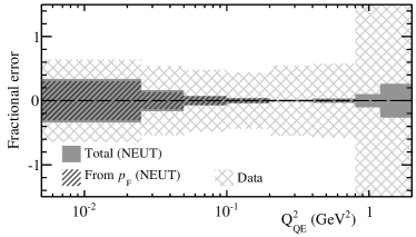
Figure 4: The fractional uncertainty on the value of $6\sigma^{\bar{\nu}}_{\mathrm{H}}/\sigma_{\mathrm{C}}^{\bar{\nu}}$ calculated for the FG model with MINER$\nu$A. The total uncertainty is obtained by combining the 1$\sigma$ uncertainties in quadrature, and the dominant uncertainty, $p_{\mathrm{F}}$ is also shown separately. The fractional uncertainty on the data is shown for comparison.

The FG model uncertainty is most significant at low $Q^{2}$ and is dominated by the uncertainty on the Fermi momentum, $p_{\mathrm{F}}$. As the model bias of our measurement is smallest at low $Q^{2}$, changing $p_{\mathrm{F}}$ may improve the $\chi^{2}$ between our measurement and the predictions of the various FG based models considered in this work. We extend the $\chi^{2}$ calculation from Equation 6 to include a variable $p_{\mathrm{F}}$ parameter with a penalty term based on the $p_{\mathrm{F}}$ uncertainty from electron-scattering data Moniz et al. (1971). The best fit $\chi^{2}$ and $p_{\mathrm{F}}$ result for each of the FG based models is shown in Table 2 for MINER$\nu$A. The fit reduces $p_{\mathrm{F}}$ slightly in order to reduce the value of $6\sigma^{\bar{\nu}}_{\mathrm{H}}/\sigma^{\bar{\nu}}_{\mathrm{C}}$ at low $Q^{2}_{\textrm{QE}}$, but there is no significant improvement in fit quality. As already commented, this study is illustrative only, modifying nuclear model uncertainties may well significantly reduce the tension for other models, but it is interesting that in the case of simple FG-based nuclear models, the tensions cannot be significantly reduced by playing with the model uncertainties.

Model	$\chi^{2}$/DOF		$p_{\mathrm{F}}$ (GeV2)
	Nominal	Fit
FG	14.8	14.1	$213.8\pm 4.0$
FG+RPA	44.3	38.2	$207.6\pm 4.0$
FG+RPA+MNP	13.6	13.5	$214.1\pm 3.9$
FG+TEM	13.4	12.8	$215.8\pm 4.5$

Table 2: Best fit $\chi^{2}$ and $p_{\mathrm{F}}$ results for the fit to FG based models for MINER$\nu$A data. The nominal $\chi^{2}$ with $p_{\mathrm{F}}$ = 217 MeV is included for comparison.

Improving the understanding of nuclear effects in neutrino scattering has become a focus for reducing systematic uncertainties in current and future neutrino oscillation experiments. As there are no current or future experiments which will take neutrino–nucleon scattering data in the few-GeV energy region, the method described here offers a unique opportunity to directly inspect the suppression or enhancement due to nuclear effects. The method exploits the fact that antineutrinos have additional interactions on free protons (from the hydrogen), and corrects for neutrino and antineutrino flux and cross section differences. It was expected to work well at low $Q^{2}$, and be relatively free of axial form factor or other uncertainties, and proves to be relatively unbiased at MINER$\nu$A even at high $Q^{2}$. Model dependent biases were seen for MiniBooNE, which should be borne in mind when applying this technique to other low energy datasets. The extracted measurement of nuclear effects in carbon is the first of its kind, and is easy to interpret for model builders. We conclude that models with nuclear screening due to long-range correlations must be balanced by the addition of multinucleon hard scattering processes, and that the combination of both effects is weakly favored over Fermi Gas models that only include the mean field of the nucleus. We also note that all of the models tested show considerable tension with the MINER$\nu$A data. Constraints from this measurement could be improved using future, higher statistics, MINER$\nu$A CCQE measurements. This method could be applied to cross section measurements in terms of different kinematic variables, although a high-$Q^{2}$ bias will remain.

I Appendix: Equality of the nuclear correction for neutrinos and antineutrinos in the Fermi Gas model

The validity of Equation 3 rests on the assumption that the ratio of bound to free cross sections is the same for neutrino and antineutrino modes. Figure 5 shows the ratio of bound to free CCQE cross sections for both neutrino ($\rho_{\nu}(E_{\nu},Q^{2})=\sigma^{\mathrm{RFG}}_{\nu}(E_{\nu},Q^{2})/\sigma^{\mathrm{free}}_{\nu}(E_{\nu},Q^{2})$) and antineutrinos ($\rho_{\bar{\nu}}(E_{\nu},Q^{2})=\sigma^{\mathrm{RFG}}_{\bar{\nu}}(E_{\nu},Q^{2})/\sigma^{\mathrm{free}}_{\bar{\nu}}(E_{\nu},Q^{2})$) assuming the RFG model in GENIE for bound nucleons as a function of $E_{\nu}$ and $Q^{2}$. The simulated events used to produce Figure 5 are flat in neutrino energy. In Figure 6, the double ratio

$$\xi(E_{\nu},Q^{2})=\frac{\sigma^{\mathrm{RFG}}_{\bar{\nu}}(E_{\nu},Q^{2})/\sigma^{\mathrm{RFG}}_{\nu}(E_{\nu},Q^{2})}{\sigma^{\mathrm{free}}_{\bar{\nu}}(E_{\nu},Q^{2})/\sigma^{\mathrm{free}}_{\nu}(E_{\nu},Q^{2})}$$ (7)

is shown, which is a direct test of this assumption for the case of the RFG model. It can be observed from Figure 5 that at the fringe of the kinematically allowed region, where Fermi motion increases the allowed phase space for the RFG model, the ratio of bound to free cross sections changes rapidly. It is clear from Figure 6 that this change is different for neutrino and antineutrino modes. This implies that there will be a bias in the test statistic defined in Equation 3 for neutrino energies which cannot populate all $Q^{2}$ bins. MINER$\nu$A, where the flux has neutrino energies in the range $1.5\leq E_{\nu}\leq 10$ GeV, will not be affected by the bias. However, MiniBooNE, with neutrino energies of $0\leq E_{\nu}\leq 3$ GeV, will be affected, although the size of this bias on the test statistic is not clear from Figure 6. The biases are shown for both MINER$\nu$A and MiniBooNE in Figure 3.

Note that the $R(Q^{2})$ defined in Equation 4 is the flux integrated $1/\xi(E_{\nu},Q^{2})$ for the case of the RFG model.

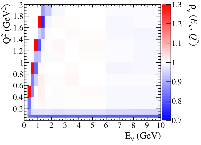
(a) Neutrino

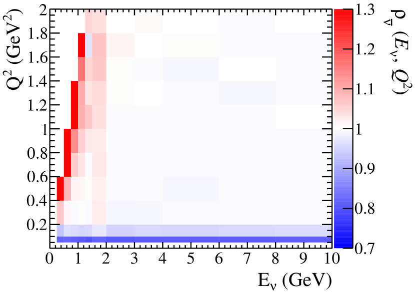
(b) Antineutrino

Figure 5: Ratios of $\sigma(E_{\nu},Q^{2})$ for the RFG and L-S models, for both neutrino and antineutrino modes.

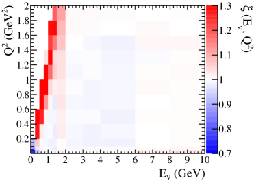
Figure 6: The double ratio $\xi(E_{\nu},Q^{2})$, defined in Equation 7, is shown. Deviations from unity indicates a bias in the technique in that region of $(E_{\nu},Q^{2})$ space.

II Appendix: Relationship between Measured $Q^{2}_{\textrm{QE}}$ and $Q^{2}$

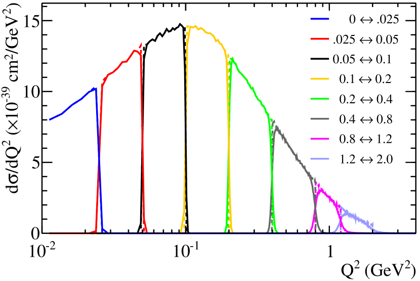
(a) MINER$\nu$A $\nu_{\mu}$–CH

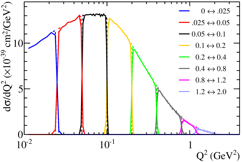
(b) MINER$\nu$A $\bar{\nu}_{\mu}$–CH

Figure 7: The $Q^{2}\rightarrow Q^{2}_{\textrm{QE}}$ smearing is shown for the MINER$\nu$A neutrino and antineutrino samples. The legend gives the $Q^{2}_{\textrm{QE}}$ bin edges used by MINER$\nu$A. The dashed lines give the flux-averaged cross section prediction for the FG model calculated using NEUT as a function of $Q^{2}_{\textrm{QE}}$ (broken down into the MINER$\nu$A binning). The solid lines show the true $Q^{2}$ distribution of events in each $Q^{2}_{\textrm{QE}}$ bin.

The $Q^{2}$ $\rightarrow$ $Q^{2}_{\textrm{QE}}$ effect for the FG model is illustrated in Figure 7 for MINER$\nu$A, and Figure 8 for MiniBooNE. In both figures, the true $Q^{2}$ distribution is shown for events which populate each of the first 8 $Q^{2}_{\textrm{QE}}$ bins of the experiments using events simulated using the FG model in NEUT with default model parameters. The smearing is not very significant for MINER$\nu$A, and is minimal in the lowest $Q^{2}_{\textrm{QE}}$ bins. For MiniBooNE, the smearing becomes significant in the higher $Q^{2}_{\textrm{QE}}$ bins (and this trend continues for the other bins not shown in Figure 8), but is minimal at low $Q^{2}_{\textrm{QE}}$. $Q^{2}_{\textrm{QE}}$ is effectively an additional smearing effect on the $Q^{2}$ distribution measured by the experiments, which is dependent on the nuclear model. As such it is part of the measurement of nuclear effects, but it will smear the bias introduced by correcting for the antineutrino/neutrino cross section difference with the L-S model. This effect is not corrected for, but is included in the bias tests shown on Figure 3. Again, it is reassuring that the $Q^{2}_{\textrm{QE}}$ smearing is minimal at low $Q^{2}$.

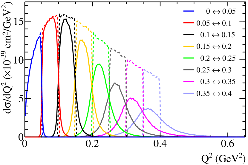
(a) MiniBooNE $\nu_{\mu}$–CH₂

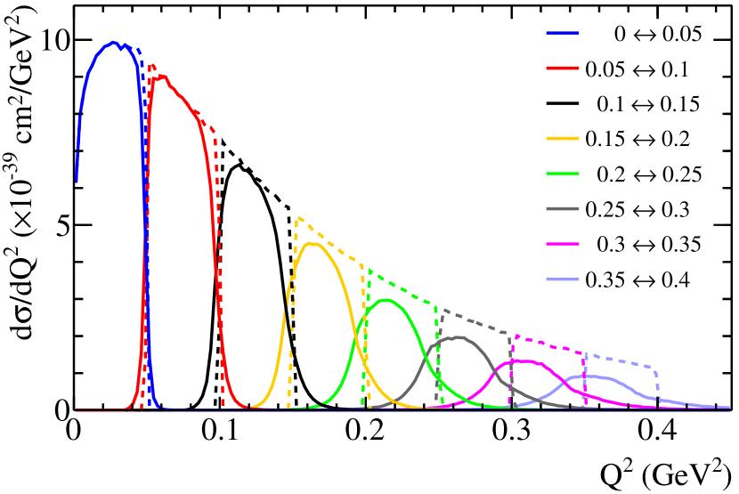
(b) MiniBooNE $\bar{\nu}_{\mu}$–CH₂

Figure 8: The $Q^{2}\rightarrow Q^{2}_{\textrm{QE}}$ smearing is shown for the first 8 bins of the MiniBooNE neutrino and antineutrino samples. The legend gives the $Q^{2}_{\textrm{QE}}$ bin edges used by MiniBooNE. The dashed lines give the flux-averaged cross section prediction for the FG model calculated using NEUT as a function of $Q^{2}_{\textrm{QE}}$ (broken down into the MiniBooNE binning). The solid lines show the true $Q^{2}$ distribution of events in each $Q^{2}_{\textrm{QE}}$ bin.

III Appendix: Applying the method to an arbitrary theoretical model

The extracted central values, $\lambda(Q^{2})=\sigma^{\bar{\nu}}_{p}(Q^{2})/\sigma^{\nu}_{n}(Q^{2})$ correction factors and covariance matrices are given for MINER$\nu$A and MiniBooNE in Tables 3 and 4 respectively. The extracted correlation matrices are also shown for both MINER$\nu$A and MiniBooNE in Figure 9. Note that no covariance matrix between the MiniBooNE bins has been released for either the neutrino or the antineutrino CCQE results; the correlations shown are due to the overall normalization uncertainties given independently for the neutrino (10.7%) and antineutrino (13.0%) data which are fully correlated between bins (but are not correlated with each other).

It is possible to apply the method outlined here to any cross section model using Equation 3, using the $\lambda(Q^{2})$ correction factor. As shown in Figure 3, the bias on the test statistic can be shown for any given model by calculating $6\sigma^{\bar{\nu}}_{\mathrm{H}}/\sigma_{\mathrm{C}}^{\bar{\nu}}$ using the test statistic defined in this work, and exactly using that model.

It is possible to form a $\chi^{2}$ statistic comparing an arbitrary model to the measurements of nuclear effects extracted here as described in Equation 6.

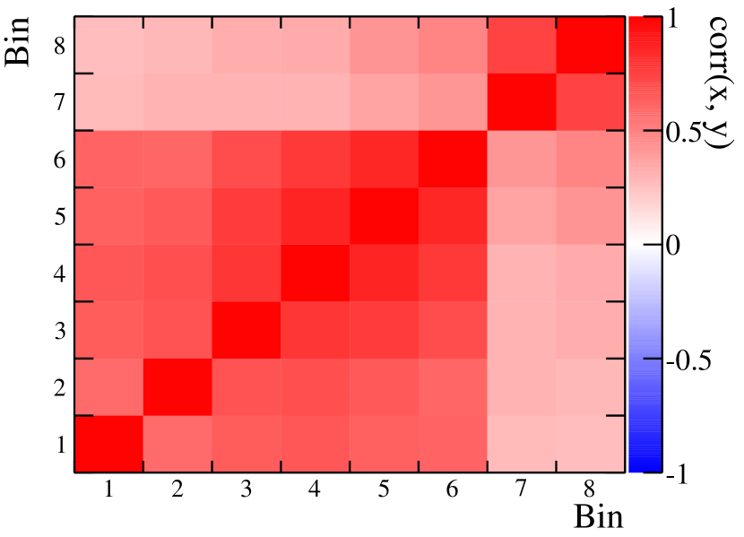
(a) MINER$\nu$A

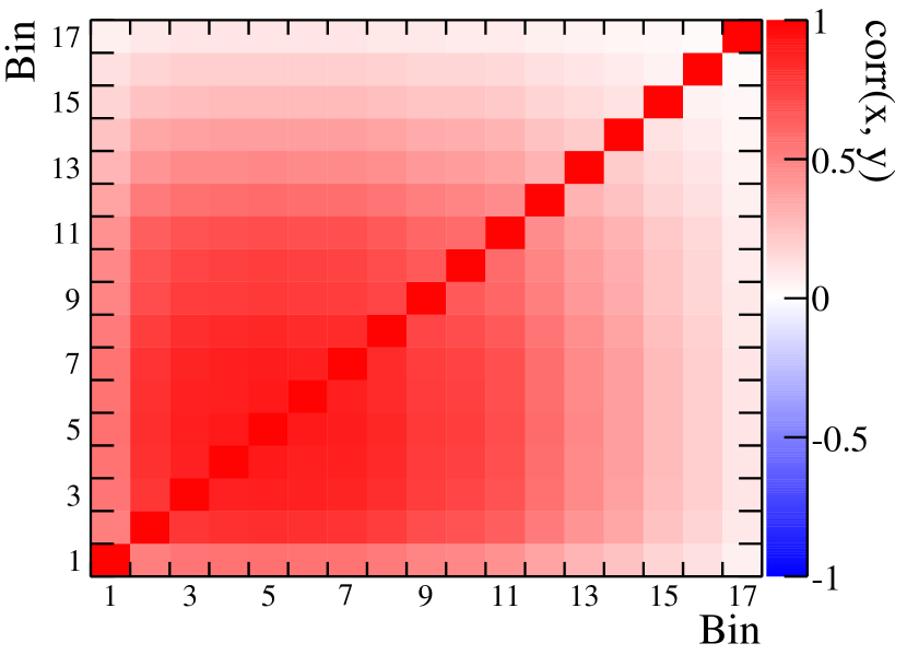
(b) MiniBooNE

Figure 9: Correlation matrices between the measurement of the test statistic extracted from data for both MINER$\nu$A and MiniBooNE. The bins numbers correspond to the increasing $Q^{2}_{\textrm{QE}}$ bins used by the experiments. The covariance matrices are given in Tables 3 and 4 for MINER$\nu$A and MiniBooNE respectively.

$Q^{2}_{\textrm{QE}}$ (GeV2) bins	0 – 0.025	0.025 – 0.05	0.05 – 0.1	0.1 – 0.2	0.2 – 0.4	0.4 – 0.8	0.8 – 1.2	1.2 – 2
Test statistic	1.61	0.83	0.85	0.22	1.06	0.89	1.66	2.49
$\lambda(Q^{2})$	0.988	0.953	0.904	0.831	0.728	0.598	0.470	0.354
0 – 0.025	0.439	0.213	0.212	0.197	0.233	0.254	0.293	0.389
0.025 – 0.05	0.213	0.306	0.186	0.172	0.204	0.210	0.275	0.356
0.05 – 0.1	0.212	0.186	0.244	0.177	0.216	0.217	0.242	0.356
0.1 – 0.2	0.197	0.172	0.177	0.201	0.218	0.219	0.221	0.331
0.2 – 0.4	0.233	0.204	0.216	0.218	0.318	0.302	0.330	0.532
0.4 – 0.8	0.254	0.210	0.217	0.219	0.302	0.388	0.423	0.677
0.8 – 1.2	0.293	0.275	0.242	0.221	0.330	0.423	2.619	2.699
1.2 – 2	0.389	0.356	0.356	0.331	0.532	0.677	2.699	4.947

Table 3: The measurement of nuclear effects on carbon using MINER$\nu$A data on $CH$, calculated using Equation 3, and the covariance matrix between the data points.

$Q^{2}_{\textrm{QE}}$ (GeV2) bins	0 – 0.05	0.05 – 0.1	0.1 – 0.15	0.15 – 0.2	0.2 – 0.25	0.25 – 0.3	0.3 – 0.35	0.35 – 0.4	0.4 – 0.45	0.45 – 0.5	0.5 – 0.6	0.6 – 0.7	0.7 – 0.8	0.8 – 1	1 – 1.2	1.2 – 1.5	1.5 – 2
Test statistic	2.49	1.59	1.27	1.29	1.39	1.33	1.22	1.39	1.45	1.61	1.64	1.42	1.4	1.38	0.93	-0.31	-1.57
$\lambda(Q^{2})$	0.784	0.543	0.408	0.321	0.262	0.217	0.186	0.162	0.141	0.125	0.108	0.090	0.077	0.064	0.052	0.043	0.037
0 – 0.05	2.093	0.609	0.568	0.570	0.583	0.574	0.561	0.583	0.591	0.613	0.616	0.587	0.585	0.582	0.522	0.358	0.190
0.05 – 0.1	0.609	0.688	0.475	0.477	0.487	0.480	0.469	0.487	0.495	0.512	0.515	0.491	0.489	0.486	0.436	0.299	0.158
0.1 – 0.15	0.568	0.475	0.516	0.444	0.454	0.447	0.437	0.454	0.461	0.477	0.480	0.457	0.455	0.453	0.407	0.279	0.148
0.15 – 0.2	0.570	0.477	0.444	0.501	0.456	0.449	0.439	0.456	0.463	0.479	0.482	0.459	0.457	0.455	0.408	0.280	0.148
0.2 – 0.25	0.583	0.487	0.454	0.456	0.511	0.459	0.449	0.466	0.473	0.490	0.493	0.469	0.468	0.465	0.417	0.286	0.152
0.25 – 0.3	0.574	0.480	0.447	0.449	0.459	0.509	0.442	0.459	0.466	0.483	0.486	0.463	0.461	0.458	0.411	0.282	0.149
0.3 – 0.35	0.561	0.469	0.437	0.439	0.449	0.442	0.495	0.449	0.455	0.471	0.474	0.452	0.450	0.448	0.402	0.275	0.146
0.35 – 0.4	0.583	0.487	0.454	0.456	0.466	0.459	0.449	0.588	0.473	0.490	0.493	0.469	0.467	0.465	0.417	0.286	0.152
0.4 – 0.45	0.591	0.495	0.461	0.463	0.473	0.466	0.455	0.473	0.712	0.497	0.500	0.476	0.474	0.472	0.424	0.290	0.154
0.45 – 0.5	0.613	0.512	0.477	0.479	0.490	0.483	0.471	0.490	0.497	0.813	0.518	0.493	0.491	0.489	0.439	0.301	0.159
0.5 – 0.6	0.616	0.515	0.480	0.482	0.493	0.486	0.474	0.493	0.500	0.518	0.952	0.496	0.494	0.492	0.441	0.302	0.160
0.6 – 0.7	0.587	0.491	0.457	0.459	0.469	0.463	0.452	0.469	0.476	0.493	0.496	1.270	0.471	0.468	0.420	0.288	0.153
0.7 – 0.8	0.585	0.489	0.455	0.457	0.468	0.461	0.450	0.467	0.474	0.491	0.494	0.471	1.892	0.466	0.419	0.287	0.152
0.8 – 1	0.582	0.486	0.453	0.455	0.465	0.458	0.448	0.465	0.472	0.489	0.492	0.468	0.466	2.800	0.416	0.285	0.151
1 – 1.2	0.522	0.436	0.407	0.408	0.417	0.411	0.402	0.417	0.424	0.439	0.441	0.420	0.419	0.416	4.462	0.256	0.136
1.2 – 1.5	0.358	0.299	0.279	0.280	0.286	0.282	0.275	0.286	0.290	0.301	0.302	0.288	0.287	0.285	0.256	4.152	0.093
1.5 – 2	0.190	0.158	0.148	0.148	0.152	0.149	0.146	0.152	0.154	0.159	0.160	0.153	0.152	0.151	0.136	0.093	4.036

Table 4: The measurement of nuclear effects on carbon using MiniBooNE data on $CH_{2}$, calculated using Equation 3, and the covariance matrix between the data points.