Distributional Behaviors of Time-averaged Observables in Langevin Equation with Fluctuating Diffusivity: Normal Diffusion but Anomalous Fluctuations

Abstract

We consider Langevin equation with dichotomously fluctuating diffusivity, where the diffusion coefficient changes dichotomously in time, in order to study fluctuations of time-averaged observables in temporary heterogeneous diffusion process. We find that occupation time statistics is a powerful tool for calculating the time-averaged mean square displacement in the model. We show that the time-averaged diffusion coefficients are intrinsically random when the mean sojourn time for one of the states diverges. Our model provides anomalous fluctuations of time-averaged diffusivity, which have relevance to large fluctuations of the diffusion coefficient in single-particle-tracking experiments.

I Introduction

Law of large numbers plays an important role in statistical physics. In stationary stochastic processes $\bm{X}_{t}$, law of large numbers or the central limit theorem tells us that time-averaged observables such as diffusivity and the ratio of occupation time converge to a constant when the measurement time goes to infinity:

$$\int_{0}^{t}O(\bm{X}_{t^{\prime}})dt^{\prime}/t\to\langle O(\bm{X})\rangle~{}{\rm as}~{}t\to\infty,$$ (1)

where the observable $O(\cdot)$ is a function of the stochastic process $\bm{X}_{t}$. In experiments, time-averaged observables are not constant because of finite measurement times. However, in some stochastic processes describing non-equilibrium phenomena, time-averaged observables are intrinsically random because of the breakdown of law of large numbers or the central limit theorem Darling and Kac (1957); Lamperti (1958). In other words, they do not converge to a constant even when the measurement time goes to infinity and the fluctuations never disappear. Such anomalous behavior has been studied by infinite ergodic theory in dynamical systems Aaronson (1997). Infinite ergodic theory states that time-averaged observables converge in distribution, and the distribution function depends on the invariant measure as well as a class of the observation function Aaronson (1981); Thaler (1998); Akimoto (2008); Akimoto et al. (2015).

Continuous-time random walk (CTRW) is a model of anomalous diffusion, where the mean square displacement (MSD) increases sub-linearly with time, and is extensively studied in disorder materials Scher and Montroll (1975) as well as biophysics He et al. (2008); Weigel et al. (2011). In CTRW, a random walker waits for the next jump and the waiting time is a random variable whose probability density function (PDF) $\rho(\tau)$ follows a power-law distribution:

$$\rho(\tau)\sim\frac{c_{0}}{|\Gamma(-\alpha)|}\tau^{-1-\alpha}\quad(\tau\to\infty),$$ (2)

where $c_{0}$ is a scale factor. When $\alpha\leq 1$, the mean waiting time diverges, thereby causing a breakdown of law of large numbers and the central limit theorem. In this case, it was shown that the time-averaged MSD (TMSD) for a fixed lag time $\Delta\ll t$, defined as

$$\overline{\delta^{2}(\Delta;t)}\equiv\frac{1}{t-\Delta}\int_{0}^{t-\Delta}dt^{\prime}\,[\bm{r}(t^{\prime}+\Delta)-\bm{r}(t^{\prime})]^{2},$$ (3)

does not converge to a constant but converges in distribution as $t\to\infty$ Lubelski et al. (2008); He et al. (2008); Akimoto and Miyaguchi (2010). Moreover, the PDF of the normalized TMSD, i.e., $\overline{\delta^{2}(\Delta;t)}/\langle\overline{\delta^{2}(\Delta;t)}\rangle$, follows a universal distribution called the Mittag-Leffler distribution, which is one of distributional limit theorems in infinite ergodic theory Akimoto and Miyaguchi (2010). This distributional property for a time-averaged observable is called distributional ergodicity in stochastic processes Miyaguchi and Akimoto (2011a); Akimoto and Miyaguchi (2013).

Other distributional behaviors have been found in other diffusion processes such as a quenched trap model Miyaguchi and Akimoto (2011b, 2015) and stored-energy-driven Levy flight (SEDLF) Akimoto and Miyaguchi (2013, 2014), where the PDF of the normalized TMSDs (time-averaged diffusion coefficients) follows other distributions depending on the power-law exponent in the waiting time distribution, the spatial dimension as well as parameters controlling jumps of a random walker. It is important to clarify whether fluctuations of time-averaged observables are intrinsic or not, because diffusion coefficients obtained by single-particle-tracking experiments in living cells exhibit large fluctuations Golding and Cox (2006); Jeon et al. (2011); Weigel et al. (2011); Tabei et al. (2013); Manzo et al. (2015). Such large fluctuations will have relevance to distributional behaviors in stochastic models of anomalous diffusion.

II Langevin equation with dichotomously fluctuating Diffusivity

To investigate ergodic properties in heterogeneous diffusion processes, we consider the following Langevin equation with fluctuating diffusivity (LEFD),

$$\frac{d\bm{r}(t)}{dt}=\sqrt{2D(t)}\bm{w}(t),$$ (4)

where $\bm{w}(t)$ is the $n$-dimensional white Gaussian noise with $\left\langle\bm{w}(t)\right\rangle=0$, and $\left\langle w_{i}(t)w_{j}(t^{\prime})\right\rangle=\delta_{ij}\delta(t-t^{\prime})$. On the other hand, the diffusion coefficient $D(t)$ can be a non-Markovian stochastic process. We assume that $D(t)$ and $\bm{w}(t)$ are statistically independent. Because the diffusion coefficient is determined by shape of the particle or surrounding environment, the LEFD can describe the dynamics of a particle with inner degree of freedom. In fact, this model can be utilized in the equation of motion for the center-of-mass of entangled polymer in reptation model Doi and Edwards (1986) and is related to dynamic heterogeneity in supercooled liquids Yamamoto and Onuki (1998a, b); Richert (2002); Helfferich et al. (2014). Moreover, because the stochastic process $D(t)$ is generic, this system includes temporally heterogeneous diffusion models induced by spacial heterogeneity such as the ones studied in Massignan et al. (2014); Chubynsky and Slater (2014); Akimoto and Seki (2015)

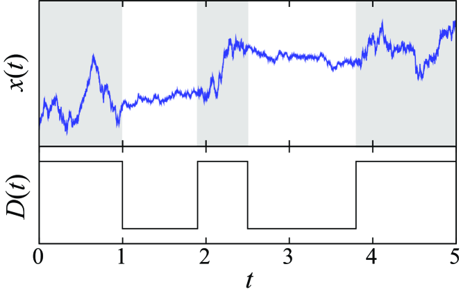
Figure 1: Trajectory of the Langevin equation with dichotomously fluctuating diffusivity. The lower inset represents the underlying diffusion coefficient.

In our previous study Uneyama et al. (2015), we have obtained the relative standard deviation (RSD) of the TMSD as a function of measurement time $t$ in LEFD when the stochastic process $D(t)$ is in equilibrium, where the RSD is defined by

$$\Sigma(t;\Delta)\equiv\frac{\sqrt{\langle[\overline{\delta^{2}(\Delta;t)}-\langle\overline{\delta^{2}(\Delta;t)}\rangle]^{2}\rangle}}{\langle\overline{\delta^{2}(\Delta;t)}\rangle}.$$ (5)

In equilibrium processes, the RSD becomes

$$\Sigma^{2}(t;\Delta)\approx\frac{2}{t^{2}}\int_{0}^{t}ds(t-s)\psi_{1}(s),$$ (6)

where $\psi_{1}(t)$ is the normalized correlation function of diffusion coefficients, i.e., $\psi_{1}(t)\equiv(\langle D(t)D(0)\rangle-\langle D\rangle^{2})/\langle D\rangle^{2}$. Therefore, information on the underlying diffusion coefficient $D(t)$ can be extracted by the RSD analysis Uneyama et al. (2012, 2015). Here, we investigate ergodic properties of LEFD especially in non-equilibrium cases. In particular, we consider two-state models for the stochastic process $D(t)$. When the mean sojourn time of a state in $D(t)$ diverges, the stochastic process becomes non-stationary, which implies that the system is intrinsically in non-equilibrium. We show normal diffusion yet anomalous fluctuations of TMSD.

Here, we consider dichotomous processes for diffusivity $D(t)$ (see Fig. 1), i.e., $D(t)=D_{+}$ if the state is $+$ and $D(t)=D_{-}$ otherwise ($-$ state). Sojourn times for $+$ and $-$ states are random variables following different probability density functions (PDFs), $\rho_{+}(\tau)$ and $\rho_{-}(\tau)$ for $+$ and $-$ states, respectively. We assume that the one of the PDFs $\rho_{+}(\tau)$ follows either a narrow distribution where all moments are finite or a broad distribution of power-law form [Eq. (2)], and that the other PDF follows a power-law distribution, whose Laplace transform is given by $\hat{\rho}_{-}(s)=1-a_{-}s^{\alpha_{-}}+o(s)$ ($\alpha_{-}<1$). In particular, we consider three cases for $\rho_{+}(x)$:

• narrow distribution:       $\hat{\rho}_{+}(s)=\sum_{k=0}^{\infty}\frac{m_{k}}{k!}s^{k}$,
  

• $\alpha_{-}<\alpha_{+}<1$:     $\hat{\rho}_{+}(s)=1-a_{+}s^{\alpha_{+}}+o(s^{\alpha_{+}})$,
  

• $\alpha_{-}=\alpha_{+}$:          $\hat{\rho}_{+}(s)=1-a_{+}s^{\alpha_{+}}+o(s^{\alpha_{+}})$,

where $m_{k}$ is the $k$th moment of sojourn times of the state $+$. In what follows, we set $\alpha_{-}=\alpha$. This kind of power-law behavior is observed in supercooled liquids Helfferich et al. (2014).

III Representation of time-averaged mean square displacement

For $\Delta\ll t$, TMSD is represented by

$$\overline{\delta^{2}(\Delta;t)}\underset{\Delta\ll t}{\approx}\!\frac{\displaystyle\sum_{i=0}^{N_{t}-1}\!\!\int_{t_{i}}^{t_{i+1}}\!\!\!\!\!\!\delta\bm{r}^{2}(\Delta;t^{\prime})dt^{\prime}+\!\int_{t_{N_{t}}}^{t}\!\!\!\!\!\delta\bm{r}^{2}(\Delta;t^{\prime})dt^{\prime}}{t},$$ (7)

where $\delta\bm{r}(\Delta;t^{\prime})\equiv\bm{r}(t^{\prime}+\Delta)-\bm{r}(t^{\prime})$, $t_{i}$ is the $i$th transition time from one state to the other state with $t_{0}=0$, $N_{t}$ is the number of transitions up to time $t$. Since a particle undergoes Brownian motion in each state,

$$\sum_{i=0}^{N_{t}-1} \int_{t_{i}}^{t_{i+1}}\delta\bm{r}^{2}(\Delta;t^{\prime})dt^{\prime}+\int_{t_{N_{t}}}^{t}\delta\bm{r}^{2}(\Delta;t^{\prime})dt^{\prime}$$

$$\underset{\Delta\ll\tau_{0}}{\approx} \int_{0}^{T_{+}(t_{N_{t}})}\!\!\!\delta\bm{r}_{+}^{2}(\Delta;t^{\prime})dt^{\prime}+\!\int_{0}^{T_{-}(t_{N_{t}})}\!\!\!\delta\bm{r}_{-}^{2}(\Delta;t^{\prime})dt^{\prime},$$ (8)

where $\delta\bm{r}_{\pm}(\Delta;t^{\prime})\equiv\int_{t^{\prime}}^{t^{\prime}+\Delta}dt^{\prime\prime}\sqrt{2D_{\pm}}\bm{w}(t^{\prime\prime})$, $T_{\pm}(t)$ is the occupation time of the state $\pm$ up to time $t$ [Thus, $T_{+}(t)+T_{-}(t)=t$], and $\tau_{0}$ is a characteristic time for the transitions of $D(t)$. The condition of $\Delta\ll\tau_{0}$ validates the approximation that the state in $[t_{i},t_{i}+\Delta]$ does not change. We have

$$\overline{\delta^{2}(\Delta;t)} \approx 2n\frac{\overline{D_{+}(t)}\,T_{+}(t)+\overline{D_{-}(t)}\,T_{-}(t)}{t}\Delta,$$ (9)

where we define a time-averaged diffusion coefficient of each state as $\overline{D_{\pm}(t)}\equiv\int_{0}^{T_{\pm}(t)}\delta\bm{r}^{2}_{\pm}(\Delta;t^{\prime})dt^{\prime}/2nT_{\pm}(t).$ Therefore, TMSDs always show normal diffusion and the time-averaged diffusion coefficient defined as $\overline{D(t)}\equiv\overline{\delta^{2}(\Delta;t)}/(2n\Delta)$ is given by

$$\overline{D(t)}\approx\overline{D_{-}(t)}+\left[\overline{D_{+}(t)}-\overline{D_{-}(t)}\right]\frac{T_{+}(t)}{t}.$$ (10)

Using Eqs. (9) and (10), we have the RSD [Eq. (5)]: $\Sigma^{2}(t;\Delta)\approx\langle[\overline{D(t)}-\langle\overline{D(t)}\rangle]^{2}\rangle/\langle\overline{D(t)}\rangle^{2}.$

In Eq. (10), the time-averaged diffusion coefficient $\overline{D(t)}$ is controlled by three stochastic variables, $\overline{D_{\pm}(t)}$, and $T_{+}(t)$. As shown below, the RSD of $T_{+}(t)$ decays slowly $t^{-\beta}$ with $\beta<1/2$ in the limit $t\to\infty$, while those of $\overline{D_{\pm}(t)}$ decay as $t^{-0.5}$. Therefore, in the long time limit, the fluctuations of $T_{+}(t)$ is dominant over those of $\overline{D_{\pm}(t)}$, and thus we can approximate as $\overline{D_{\pm}(t)}\simeq D_{\pm}$. Under this approximation, we have an asymptotic behavior of the RSD:

$$\Sigma^{2}(t;\Delta)\sim\frac{\left\langle T_{+}^{2}(t)\right\rangle-\left\langle T_{+}(t)\right\rangle^{2}}{\frac{D_{-}}{(D_{+}-D_{-})^{2}}t^{2}+\langle T_{+}(t)\rangle^{2}}.$$ (11)

This is another representation of the RSD by the occupation time in LEFD with two-state diffusivity. We confirmed that the asymptotic behavior is the same as the RSD (6) in equilibrium processes. Since we neglect fluctuations of $\overline{D_{\pm}(t)}$, this expression for the RSD is valid only when the right-hand side of Eq. (11) decays slower than $t^{-0.5}$. Otherwise, the asymptotic behavior of the RSD is the same as that in Brownian motion (see Appendix. A):

$$\Sigma^{2}(t;\Delta)\sim\frac{\langle(\overline{D_{-}(t)}-D_{-})^{2}\rangle}{D_{-}^{2}}\sim\frac{4\Delta}{3nt}.$$ (12)

IV Occupation time statics

Here, we consider the occupation time statics for three cases. We define the joint probability distribution, $g^{\pm}_{n}(y;t)$, of the occupation time $T_{+}(t)=y$ and the number of renewal $N_{t}=n$ up to time $t$ under the condition that the initial state is $\pm$, given by

$$g^{\pm}_{n}(y;t)=\left\langle\delta\left(y-T_{+}(t)\right)I\left(t_{n}\leq t<t_{n+1}\right)\right\rangle_{\pm}.$$ (13)

The Laplace transform of $g^{\pm}_{n}(y;t)$ with respect to $y$ and $t$ is given by

$$\hat{g}^{\pm}_{n}(u;s)=\left\langle\int_{t_{n}}^{t_{n+1}}e^{-st}e^{-uT_{+}(t)}dt\right\rangle_{\pm},$$ (14)

where $n=1,2,\dots$. For example, if the initial state is $+$ and $n=2k$ or $2k+1$, it can be represented as

$$\hat{g}^{\pm}_{2k}(u;s) =\left\langle\int_{t_{2k}}^{t_{2k+1}}\!\!\!e^{-st}e^{-u[\tau_{1}+\tau_{3}+\dots+\tau_{2k-1}+(t-t_{2k})]}dt\right\rangle,$$ (15)

$$\hat{g}^{\pm}_{2k+1}(u;s) =\left\langle\int_{t_{2k+1}}^{t_{2k+2}}\!\!\!e^{-st}e^{-u(\tau_{1}+\tau_{3}+\dots+\tau_{2k+1})}dt\right\rangle,$$ (16)

where $\tau_{k}$ is the $k$th sojourn time, and thus $t_{k}=\sum_{i=1}^{k}\tau_{i}$. Integrating the above equations, and using interindependence of $\tau_{k}$ and $\tau_{l}$ ($k\neq l$), we have

$$\hat{g}^{+}_{2k+1}(u;s) =\frac{1-\hat{\rho}_{-}(s)}{s}\hat{\rho}_{-}^{k}(s)\hat{\rho}_{+}^{k+1}(s+u),$$ (17)

$$\hat{g}^{+}_{2k}(u;s) =\frac{1-\hat{\rho}_{+}(s+u)}{s+u}\hat{\rho}_{-}^{k}(s)\hat{\rho}_{+}^{k}(s+u).$$ (18)

The cases in which the system starts from $-$ state can be calculated in the similar way. Then, the the PDF of $T_{+}(t)$ is obtained by summing up $g^{\pm}_{n}(y;t)$ in terms of $n$: ${g}^{\pm}(y;t)=\sum_{n=0}^{\infty}g^{\pm}_{n}(y;t)$, and thus we have

$$\hat{g}^{+}(u;s) =\frac{1-\hat{\rho}_{-}(s)}{s\hat{\rho}(s,u)}\hat{\rho}_{+}(s+u)+\frac{1-\hat{\rho}_{+}(s+u)}{(s+u)\hat{\rho}(s,u)},$$ (19)

$$\hat{g}^{-}(u;s) =\frac{1-\hat{\rho}_{+}(s+u)}{(s+u)\hat{\rho}(s,u)}\hat{\rho}_{-}(s)+\frac{1-\hat{\rho}_{-}(s)}{s\hat{\rho}(s,u)},$$ (20)

where $\rho(s,u)\equiv 1-\hat{\rho}_{+}(s+u)\hat{\rho}_{-}(s)$. In the small $s$ and $u$ limit,

$$\hat{g}^{\pm}(u;s) \sim\frac{1-\hat{\rho}_{-}(s)}{s\hat{\rho}(s,u)}+\frac{1-\hat{\rho}_{+}(s+u)}{(s+u)\hat{\rho}(s,u)}.$$ (21)

V Distributional limit theorems

V.1 Case (1)

From Eq. (21), the Laplace transform of the PDF of $T_{+}(t)$ for the case (1) is given by

$$\hat{g}^{\pm}(u;s)\sim\frac{a_{-}s^{\alpha-1}+\mu_{+}}{a_{-}s^{\alpha}+\mu_{+}(s+u)}.$$ (22)

Using the relation between the moments of $T_{+}(t)$ and $\hat{g}^{\pm}(u;s)$, we have the asymptotic behavior of the $n$th moment of $T_{+}(t)$

$$\left\langle T_{+}^{n}(t)\right\rangle_{\pm} \sim\left(\frac{\mu}{a_{-}}\right)^{\!\!n}\!\!\frac{n!\,t^{n\alpha}}{\Gamma(1+n\alpha)},$$ (23)

where $\mu=m_{1}$. It follows that the ETMSD shows normal diffusion:

$$\langle\overline{\delta^{2}(\Delta;t)}\rangle\sim 2n\left[D_{-}+\frac{\mu(D_{+}-D_{-})}{a_{-}\Gamma(1+\alpha)}\frac{1}{t^{1-\alpha}}\right]\Delta,$$ (24)

where we used $\langle\overline{D_{\pm}(t)}\rangle\sim D_{\pm}$ and Eq. (23). Because TMSD converges to $2nD_{-}\Delta$ as $t\to\infty$, this process seems to be normal diffusion.

In Brownian motion, $\overline{D(t)}$ converges to a constant and the distribution follows Gaussian. Thus, deviation from Gaussian detects anomaly of the process. Since $\overline{D(t)}$ is given by Eq. (10) and $\overline{D(t)}\to D_{-}$, we consider the deviation, i.e., $\delta D_{t}\equiv\overline{D(t)}-D_{-}$. By Eq. (10), we have

$$\frac{\delta D_{t}}{\langle\delta D_{t}\rangle}\cong\frac{(\overline{D_{-}(t)}-D_{-})t}{(D_{+}-D_{-})\langle T_{+}(t)\rangle}+\frac{T_{+}(t)}{\langle T_{+}(t)\rangle}.$$ (25)

Here, the first term in the right-hand side can be neglected if $\langle(\overline{D_{-}(t)}-D_{-})^{2}t^{2}\rangle=o(\langle T_{+}(t)^{2}\rangle-\langle T_{+}(t)\rangle^{2}$). Note that this condition is satisfied when $\alpha>0.5$ [see Eq. (23)]. By Eq. (23), moments of the normalized occupation time defined by $T_{\alpha}(t)\equiv T_{+}(t)/\langle T_{+}(t)\rangle$ becomes

$$\langle T_{\alpha}(t)^{n}\rangle\sim\frac{n!\Gamma(1+\alpha)^{n}}{\Gamma(1+n\alpha)}\quad(t\to\infty).$$ (26)

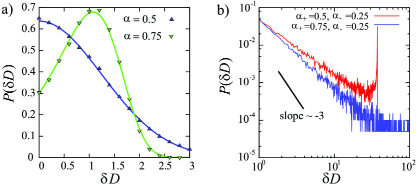
When the PDF of a random variable $M_{\alpha}$ follows the Mittag-Leffler distribution of order $\alpha$, the Laplace transform is given by $\langle e^{-zM_{\alpha}}\rangle=\sum_{k=0}^{\infty}\frac{\Gamma(1+\alpha)^{k}z^{k}}{\Gamma(1+k\alpha)}.$Therefore, the distribution of $\delta D_{t}/\langle\delta D_{t}\rangle$ is not Gaussian but converges to the Mittag-Leffler distribution when $\alpha>0.5$ (see Fig. 2a). For $\alpha<0.5$, the first term in Eq. (25) becomes the leading term and the distribution of $\delta D_{t}/\langle\delta D_{t}\rangle$ becomes Gaussian with the mean 0 and the variance $2\Delta D_{-}^{2}a_{-}^{2}\Gamma(1+\alpha)^{2}t^{1-2\alpha}/\{n(D_{+}-D_{-})^{2}\mu^{2}\}$. For $\alpha>0.5$, using Eq. (11) yields

$$\Sigma^{2}(t;\Delta)\sim\frac{\mu^{2}(D_{+}-D_{-})^{2}A(\alpha)}{a_{-}^{2}D_{-}^{2}\Gamma(1+\alpha)^{2}}t^{-(1-\alpha)},$$ (27)

where $A(\alpha)=\frac{2\Gamma(\alpha+1)^{2}}{\Gamma(2\alpha+1)}-1$. For $D_{-}=0$, the result is exactly the same as that in CTRW He et al. (2008): $\Sigma(t;\Delta)\sim\sqrt{A(\alpha)}.$

V.2 Case (2)

In this case, Eq. (21) yields the Laplace transform of the PDF of $T_{+}(t)$:

$$\hat{g}^{\pm}(u;s)\sim\frac{a_{+}(s+u)^{\alpha_{+}-1}+a_{-}s^{\alpha-1}}{a_{+}(s+u)^{\alpha_{+}}+a_{-}s^{\alpha}}.$$ (28)

The Laplace transform of the first moment $\langle T_{+}(t)\rangle$ is scaled as

$$\langle\hat{T}_{+}(s)\rangle=\left.\frac{\partial\hat{g}^{\pm}(u;s)}{\partial u}\right|_{u=0}\sim-\frac{a_{+}}{a_{-}}\frac{1}{s^{2-\delta-\alpha}},$$ (29)

where $\delta\alpha=\alpha_{+}-\alpha$. Thus, The asymptotic behavior of $\langle T_{+}(t)\rangle$ becomes

$$\langle T_{+}(t)\rangle\sim\frac{a_{+}}{a_{-}\Gamma(2-\delta\alpha)}t^{1-\delta\alpha},$$ (30)

Moreover, the second moment of $T_{+}(t)$ is scaled as

$$\langle T_{+}(t)^{2}\rangle\sim\frac{2a_{+}(1-\alpha_{+})}{a_{-}\Gamma(3-\delta\alpha)}t^{2-\delta\alpha}.$$ (31)

It follows that the second moment of $T_{+}(t)/\langle T_{+}(t)\rangle$ diverges for $t\to\infty$. Using Eqs. (10) and (30) yields the ETMSD:

$$\langle\overline{\delta^{2}(\Delta;t)}\rangle\sim 2n\left[D_{-}+\frac{a_{+}(D_{+}-D_{-})}{a_{-}\Gamma(2-\alpha_{+}+\alpha)}\frac{1}{t^{\alpha_{+}-\alpha}}\right]\Delta.$$ (32)

As in the previous case, TMSD converges to $2nD_{-}\Delta$ as $t\to\infty$. By Eq. (11), the RSD decays as

$$\Sigma^{2}(t;\Delta)\sim\frac{2a_{+}(D_{+}-D_{-})^{2}(1-\alpha_{+})}{a_{-}D_{-}^{2}\Gamma(3-\delta\alpha)}t^{-\delta\alpha}.$$ (33)

Although we do not have the limit distribution of $T_{+}(t)/\langle T_{+}(t)\rangle$, the tail should be a heavy tail (power-law distribution) because the second moment of $T_{+}(t)/\langle T_{+}(t)\rangle$ diverges. By the relation between $\delta D_{t}$ and $T_{+}(t)$, i.e., Eq. (25), we find that the deviations of time-averaged diffusion coefficient, $\delta D_{t}/\langle\delta D_{t}\rangle$, are random and the distribution is a non-trivial distribution characterized by a power law (see Fig. 2b). This is a similar situation for the PDF of time-averaged diffusion coefficients in some parameter region of SEDLF Akimoto and Miyaguchi (2014).

Figure 2: Distribution of deviations of the time-averaged diffusivity, $\delta D\equiv\delta D_{t}/\langle D_{t}\rangle$, in the cases (1) and (2), corresponding to (a) and (b), respectively ($D_{-}=1$, $D_{+}=10$, and $t=10^{4}$). In Fig. (a), the Mittag-Leffler distributions are drawn by solid lines. In Fig. (b), power-law distribution with exponent $-3$ is drawn for reference. Squares with colors are the results of numerical simulations. In numerical simulations, we used the following power-law distribution for sojourn time distribution: $\rho_{\pm}(\tau)=c_{\pm}\tau^{-1-\alpha_{\pm}}$ for $\tau\geq\tau_{0}^{\pm}$ and $0$ for $\tau<\tau_{0}^{\pm}$, where $c_{\pm}$ is the normalization constant. In case (1), we used the exponential distribution for $\rho_{+}(\tau)$.

V.3 Case (3)

Contrary to the previous two cases, TMSDs do not converge to a constant in the case (3), whereas TMSD shows normal diffusion [see Eq. (9)]. Eq. (21) yields the Laplace transform of the PDF of $T_{+}(t)$:

$$\hat{g}^{\pm}(u;s)\sim\frac{a_{+}(s+u)^{\alpha-1}+a_{-}s^{\alpha-1}}{a_{+}(s+u)^{\alpha}+a_{-}s^{\alpha}}.$$ (34)

By Appendix B in Godrèche and Luck (2001), Eq. (34) implies that the limit distribution of $T^{+}(t)/t$ exists:

$$\lim_{t\to\infty}g_{T^{+}/t}(x)=g_{\alpha,\beta}(x),$$ (35)

and the distribution is given by

$$g_{\alpha,\beta}(x)=\frac{(a\sin\pi\alpha/\pi)x^{\alpha-1}(1-x)^{\alpha-1}}{a^{2}x^{2\alpha}+2a\cos\pi\alpha(1-x)^{\alpha}x^{\alpha}+(1-x)^{2\alpha}},$$ (36)

where $g_{T^{+}/t}(x)$ is the PDF of $T_{+}(t)/t$, $a=a_{-}/a_{+}$ and $\beta\equiv 1/(1+a)$. This is the Lamperti’s generalized arcsine law Lamperti (1958), which is observed for time-averaged drift in superdiffusion Akimoto (2012). By Eq. (10), the distribution of the time-averaged diffusion coefficient is given by that of $T_{+}(t)/t$:

$$\Pr\left(\overline{D(t)}\leq x\right) = \Pr\left(\frac{T_{+}(t)}{t}\leq\frac{x-D_{-}}{D_{+}-D_{-}}\right).$$ (37)

Because the PDF of $T_{+}(t)/t$ follows the Lamperti’s generalized arcsine law, Eq. (36), the PDF of $\overline{D(t)}$ is given by $P_{D}(x)=g_{\alpha,\beta}\left(\frac{x-D_{-}}{D_{d}}\right)/D_{d},$ where $D_{d}=D_{+}-D_{-}$. Because the mean and second moment of $T_{+}(t)/t$ are given by $\langle T_{+}(t)/t\rangle=\beta$ and $\langle(T_{+}/t)^{2}\rangle=m(\alpha,\beta)\equiv\beta(\alpha\beta+1-\alpha)$, respectively Godrèche and Luck (2001), we have the RSD

$$\Sigma(t;\Delta)\sim\sqrt{\frac{D_{-}^{2}+2D_{-}D_{d}\beta+D_{d}^{2}m(\alpha,\beta)}{(D_{-}+D_{d}\beta)^{2}}-1}.$$ (38)

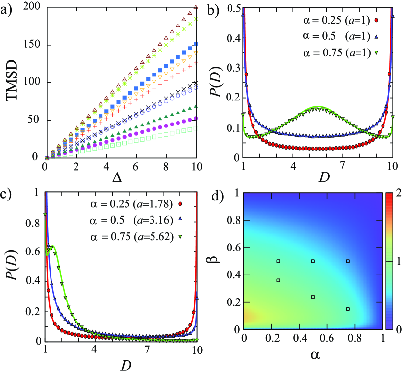
As shown in Fig. 3, theory is in good agreement with numerical results.

Figure 3: Anomalous fluctuations of time-averaged diffusivity in the case 3 ($D_{-}=1$ and $D_{+}=10$). (a) TMSDs for 10 different realizations ($\alpha=0.5$ and $t=10^{4}$). (b) and (c) Distribution of time-averaged diffusion coefficients ($t=10^{3}$). Symbols are the results of numerical simulations and solid curves are the theoretical ones. (d) RSD as a function of $\alpha$ and $\beta$ ($t=10^{5}$). Squares with colors are the results of numerical simulations. In numerical simulations, we used the same power-law distribution as in Fig. 2.

VI Conclusion

We have shown three distributional limit theorems for time-averaged observables related to diffusivity in the Langevin equation with dichotomously fluctuating diffusivity. When one of the states is zero ($D_{-}=0$) in the case (1), statistical properties of TMSD are exactly the same as those in CTRW. Therefore, this model is a generalization of CTRW. When both diffusion coefficients are not zero, the TMSD asymptotically show normal diffusion in all cases, whereas fluctuations of TMSD (deviations of time-averaged diffusion coefficients) are intrinsically random. Especially in case (3), time-averaged diffusion coefficients are intrinsically random and the distribution follows the generalized arcsine law. As a result, we have found anomalous fluctuations in apparently normal diffusion processes.

Appendix A Derivation of Eq. (12)

Here, we derive the RSD in Brownian motion with the diffusion coefficient $D_{-}$. Since this process is described by Brownian motion, displacement $\delta\bm{r}(\Delta;t)\equiv\bm{r}(\Delta+t)-\bm{r}(t)$ follows a Gaussian distribution with the mean 0 and the variance $2nD_{-}\Delta$. The mean TMSD is straightforwardly calculated as $\langle\{\overline{\delta^{2}(\Delta;t)}\}\rangle=2nD_{-}\Delta$. The second moment of TMSD can be calculated as follows:

$$\langle\{\overline{\delta^{2}(\Delta;t)}\}^{2}\rangle \sim\frac{2}{t^{2}}\int_{0}^{t}dt^{\prime}\int_{t^{\prime}}^{t}dt^{\prime\prime}\langle\delta\bm{r}^{2}(\Delta;t^{\prime})\delta\bm{r}^{2}(\Delta;t^{\prime\prime})\rangle$$ (39)

$$=\frac{2}{t^{2}}\int_{0}^{t}dt^{\prime}\int_{t^{\prime}}^{t^{\prime}+\Delta}dt^{\prime\prime}\langle\delta\bm{r}^{2}(\Delta;t^{\prime})\delta\bm{r}^{2}(\Delta;t^{\prime\prime})\rangle+\frac{2}{t^{2}}\int_{0}^{t}dt^{\prime}\int_{t^{\prime}+\Delta}^{t}dt^{\prime\prime}\langle\delta\bm{r}^{2}(\Delta;t^{\prime})\rangle\langle\delta\bm{r}^{2}(\Delta;t^{\prime\prime})\rangle$$ (40)

$$=\frac{2}{t^{2}}\int_{0}^{t}dt^{\prime}\int_{t^{\prime}}^{t^{\prime}+\Delta}dt^{\prime\prime}\left\{\langle\delta\bm{r}^{2}(t^{\prime\prime}-t^{\prime};t^{\prime})\rangle\langle\delta\bm{r}^{2}(\Delta;t^{\prime\prime})\rangle+\langle\delta\bm{r}^{4}(t^{\prime}+\Delta-t^{\prime\prime};t^{\prime\prime})\rangle\right.$$ (41)

$$+\langle\delta\bm{r}^{2}(t^{\prime}+\Delta-t^{\prime\prime};t^{\prime\prime})\rangle\langle\delta\bm{r}^{2}(t^{\prime\prime}-t^{\prime};t^{\prime}+\Delta)\rangle\}+\frac{2}{t^{2}}\int_{0}^{t}dt^{\prime}(t-t^{\prime}-\Delta)(2nD\Delta)^{2}$$ (42)

$$=(2nD\Delta)^{2}\left(1+\frac{4\Delta}{3nt}\right).$$ (43)

It follows that the RSD decays as

$$\Sigma^{2}(t;\Delta)\sim\frac{4\Delta}{3nt}\quad(t\to\infty).$$ (44)

References

• Darling and Kac (1957) D. A. Darling and M. Kac, Trans. Am. Math. Soc. 84, 444 (1957).
• Lamperti (1958) J. Lamperti, Trans. Am. Math. Soc. 88, 380 (1958).
• Aaronson (1997) J. Aaronson, An Introduction to Infinite Ergodic Theory (American Mathematical Society, Providence, 1997).
• Aaronson (1981) J. Aaronson, J. D’Analyse Math. 39, 203 (1981).
• Thaler (1998) M. Thaler, Trans. Am. Math. Soc. 350, 4593 (1998).
• Akimoto (2008) T. Akimoto, J. Stat. Phys. 132, 171 (2008).
• Akimoto et al. (2015) T. Akimoto, S. Shinkai,  and Y. Aizawa, J. Stat. Phys. 158, 476 (2015).
• Scher and Montroll (1975) H. Scher and E. W. Montroll, Phys. Rev. B 12, 2455 (1975).
• He et al. (2008) Y. He, S. Burov, R. Metzler,  and E. Barkai, Phys. Rev. Lett. 101, 058101 (2008).
• Weigel et al. (2011) A. Weigel, B. Simon, M. Tamkun,  and D. Krapf, Proc. Natl. Acad. Sci. USA 108, 6438 (2011).
• Lubelski et al. (2008) A. Lubelski, I. M. Sokolov,  and J. Klafter, Phys. Rev. Lett. 100, 250602 (2008).
• Akimoto and Miyaguchi (2010) T. Akimoto and T. Miyaguchi, Phys. Rev. E 82, 030102(R) (2010).
• Miyaguchi and Akimoto (2011a) T. Miyaguchi and T. Akimoto, Phys. Rev. E 83, 062101 (2011a).
• Akimoto and Miyaguchi (2013) T. Akimoto and T. Miyaguchi, Phys. Rev. E 87, 062134 (2013).
• Miyaguchi and Akimoto (2011b) T. Miyaguchi and T. Akimoto, Phys. Rev. E 83, 031926 (2011b).
• Miyaguchi and Akimoto (2015) T. Miyaguchi and T. Akimoto, Phys. Rev. E 91, 010102 (2015).
• Akimoto and Miyaguchi (2014) T. Akimoto and T. Miyaguchi, J. Stat. Phys. 157, 515 (2014).
• Golding and Cox (2006) I. Golding and E. C. Cox, Phys. Rev. Lett. 96, 098102 (2006).
• Jeon et al. (2011) J.-H. Jeon, V. Tejedor, S. Burov, E. Barkai, C. Selhuber-Unkel, K. Berg-Sørensen, L. Oddershede,  and R. Metzler, Phys. Rev. Lett. 106, 048103 (2011).
• Tabei et al. (2013) S. A. Tabei, S. Burov, H. Y. Kim, A. Kuznetsov, T. Huynh, J. Jureller, L. H. Philipson, A. R. Dinner,  and N. F. Scherer, Proc. Natl. Acad. Sci. USA 110, 4911 (2013).
• Manzo et al. (2015) C. Manzo, J. A. Torreno-Pina, P. Massignan, G. J. Lapeyre Jr, M. Lewenstein,  and M. F. G. Parajo, Phys. Rev. X 5, 011021 (2015).
• Doi and Edwards (1986) M. Doi and S. F. Edwards, The Theory of Polymer Dynamics (Oxford University Press, Oxford, 1986).
• Yamamoto and Onuki (1998a) R. Yamamoto and A. Onuki, Phys. Rev. Lett. 81, 4915 (1998a).
• Yamamoto and Onuki (1998b) R. Yamamoto and A. Onuki, Phys. Rev. E 58, 3515 (1998b).
• Richert (2002) R. Richert, J. Phys. Cond. Matt. 14, R703 (2002).
• Helfferich et al. (2014) J. Helfferich, F. Ziebert, S. Frey, H. Meyer, J. Farago, A. Blumen,  and J. Baschnagel, Phys. Rev. E 89, 042603 (2014).
• Massignan et al. (2014) P. Massignan, C. Manzo, J. A. Torreno-Pina, M. F. García-Parajo, M. Lewenstein,  and J. G. J. Lapeyre, Phys. Rev. Lett. 112, 150603 (2014).
• Chubynsky and Slater (2014) M. V. Chubynsky and G. W. Slater, Phys. Rev. Lett. 113, 098302 (2014).
• Akimoto and Seki (2015) T. Akimoto and K. Seki, Phys. Rev. E 92, 022114 (2015).
• Uneyama et al. (2015) T. Uneyama, T. Miyaguchi,  and T. Akimoto, Phys. Rev. E 92, 032140 (2015).
• Uneyama et al. (2012) T. Uneyama, T. Akimoto,  and T. Miyaguchi, J. Chem. Phys. 137, 114903 (2012).
• Godrèche and Luck (2001) C. Godrèche and J. M. Luck, J. Stat. Phys. 104, 489 (2001).
• Akimoto (2012) T. Akimoto, Phys. Rev. Lett. 108, 164101 (2012).