Vector and axial vector mesons
in a nonlocal chiral quark model

Abstract

Basic features of nonstrange vector and axial vector mesons are analyzed in the framework of a chiral quark model that includes nonlocal four-fermion couplings. Unknown model parameters are determined from some input values of masses and decay constants, while nonlocal form factors are taken from a fit to lattice QCD results for effective quark propagators. Numerical results show a good agreement with the observed meson phenomenology.

I Introduction

Given the nonperturbative character of quantum chromodynamics (QCD) in the low-energy regime, the analysis of hadron phenomenology starting from first principles is still a challenge for theoretical physics. Although substantial progress has been achieved in this sense through lattice QCD (LQCD) calculations, this approach shows significant difficulties, e.g. when dealing with small quark masses or with hadronic systems at nonzero chemical potentials. Thus it is important to study the consistency between the results obtained through lattice calculations and those arising from effective models for strongly interacting particles. For two light flavors it is believed that QCD supports an approximate SU(2) chiral symmetry that is dynamically broken at low energies, where pions play the role of the corresponding Goldstone bosons. The well-known Nambu$-$Jona-Lasinio (NJL) model njl ; njlrev , in which light mesons are described as fermion-antifermion composite states, is a simple effective approach that shows these features. In the NJL model quarks interact through a local four-fermion coupling, leading to relatively simple Schwinger-Dyson and Bethe-Salpeter equations. Now, as a step toward a more realistic approach to low-energy QCD, it is worth it to consider extensions of the NJL model that include nonlocal interactions ripka . In particular, this is supported by lattice calculations, which lead to a given momentum dependence of both the mass and the wave function renormalization (WFR) in the effective quark propagators Parappilly:2005ei ; Furui:2006ks . It is also seen that nonlocal extensions of the NJL model do not exhibit some problems that are present in the local theory. For example, nonlocal interactions regularize the model in such a way that the effective interaction is finite to all orders in the loop expansion, thus model predictions are less dependent on the parameterizations, and there is no need to introduce extra cutoffs Blaschke:1995gr .

Previous works on nonlocal NJL-like (nlNJL) models, focused on different aspects of strong interaction physics, can be found in the literature. These include the study of vacuum hadronic properties considering either two Schmidt:1994di ; BB95 ; Plant:1997jr ; Golli:1998rf ; Noguera:2005ej ; GomezDumm:2006vz ; Noguera:2008 ; Costa:2010pp or three Scarpettini:2003fj active quark flavors, and various nonlocal form factor shapes. In addition, this framework has been used to describe the chiral restoration transition for hadronic systems at finite temperature and/or chemical potential (see e.g. Refs. GomezDumm:2001fz ; Hell:2008cc ; Radzhabov:2010dd ; Contrera:2010kz ; Hell:2011ic ; Carlomagno:2013ona ). In this work, following the proposal in Refs. Noguera:2005ej ; Noguera:2008 , we consider a model in which nonlocal form factors lead to a momentum dependence of the mass and WFR in the quark propagator, hence the actual shape of these form factors can be taken from the data obtained through lattice calculations Noguera:2008 ; Contrera:2010kz . We concentrate here in particular in the incorporation of explicit vector and axial vector interactions. Therefore, besides the previously considered couplings between scalar and pseudoscalar quark-antiquark currents, in our model we include couplings between vector and axial vector nonlocal currents satisfying proper QCD symmetry requirements. In fact, nonlocal models including vector and axial vector currents have been previously considered in Ref. Plant:1997jr . However, those models do not include a momentum-dependent WFR of quark propagators, which is required in order to perform the comparison with lattice QCD results. We dedicate the first part of the paper to work out the formalism in order to derive analytical expressions for some basic vector meson properties, such as masses and decay parameters. Then we present numerical results obtained by taking the nonlocal form factors from a fit to lattice QCD data. It is seen that, after fixing unknown coupling constants so as to reproduce some input meson observables, the model provides an adequate phenomenological description of the considered vector meson properties.

The article is organized as follows. In Sect. 2 we introduce the model and derive the corresponding gap equations at the mean field level. In Sect. 3 we describe the vector meson sector, obtaining analytical results for meson masses and decay amplitudes. The numerical and phenomenological analyses are included in Sect. 4, while in Sect. 5 we present a summary of our work. Finally, in Appendixes A and B we collect some analytical expressions and describe the calculation procedure.

II Model

We consider a two-flavor chiral quark model that includes nonlocal vector and axial vector quark-antiquark currents. Since our aim is to choose form factors that are in agreement with LQCD calculations, it is convenient to work in Euclidean space, where nonlocal interactions are well defined ripka . The corresponding effective action is given by

$$S_{E} = \int d^{4}x\ \left\{\bar{\psi}(x)(-\,i\not{\partial}+\hat{m})\psi(x)-\frac{G_{S}}{2}\Big{[}j_{S}(x)j_{S}(x)+\vec{j}_{P}(x)\cdot\vec{j}_{P}(x)+j_{M}(x)j_{M}(x)\Big{]}\right.$$ (1)

$$\left.-\,\frac{G_{V}}{2}\Big{[}\vec{j}_{V}^{\,\mu}(x)\cdot\vec{j}_{V\mu}(x)+\vec{j}_{A}^{\,\mu}(x)\cdot\vec{j}_{A\,\mu}(x)\Big{]}-\frac{G_{0}}{2}\;j^{\,0\,\mu}_{V}(x)j^{\,0}_{V\mu}(x)-\frac{G_{5}}{2}\;j_{A}^{\,0\,\mu}(x)j^{\,0}_{A\,\mu}(x)\right\}\ ,$$

where $\psi(x)$ is the $N_{f}=2$ quark doublet, $\psi=(u\ d)^{T}$, and $\hat{m}={\rm diag}(m_{u},m_{d})$ is the current quark mass matrix. We will work in the isospin symmetry limit, assuming $m_{u}=m_{d}$, which will be called from now on $m_{c}$. The fermion currents are given by Noguera:2008

$$j_{S}(x) = \int d^{4}z\;g(z)\,\bar{\psi}\left(x+\frac{z}{2}\right)\psi\left(x-\frac{z}{2}\right)\ ,$$

$$j_{P}^{a}(x) = \int d^{4}z\;g(z)\,\bar{\psi}\left(x+\frac{z}{2}\right)i\,\gamma_{5}\,\tau^{a}\psi\left(x-\frac{z}{2}\right)\ ,$$

$$j_{M}(x) = \frac{1}{2\varkappa}\;\int d^{4}z\;f(z)\,\bar{\psi}\left(x+\frac{z}{2}\right)\,i\overleftrightarrow{\not{\partial}}\psi\left(x-\frac{z}{2}\right)\ ,$$

$$j_{V\mu}^{a}(x) = \int d^{4}z\;h(z)\,\bar{\psi}\left(x+\frac{z}{2}\right)\tau^{a}\gamma_{\mu}\psi\left(x-\frac{z}{2}\right)\ ,$$

$$j_{A\,\mu}^{a}(x) = \int d^{4}z\;h(z)\,\bar{\psi}\left(x+\frac{z}{2}\right)\tau^{a}\gamma_{\mu}\gamma_{5}\psi\left(x-\frac{z}{2}\right)\ ,$$

$$j^{\,0}_{V\mu}(x) = \int d^{4}z\;h_{0}(z)\,\bar{\psi}\left(x+\frac{z}{2}\right)\gamma_{\mu}\psi\left(x-\frac{z}{2}\right)\ ,$$

$$j^{\,0}_{A\,\mu}(x) = \int d^{4}z\;h_{5}(z)\,\bar{\psi}\left(x+\frac{z}{2}\right)\gamma_{\mu}\gamma_{5}\psi\left(x-\frac{z}{2}\right)\ ,$$ (2)

where $\tau^{a}$, $a=1,2,3$, are the Pauli matrices, while $u(x^{\prime})\overleftrightarrow{\partial}v(x)\equiv u(x^{\prime})\partial_{x}v(x)-\partial_{x^{\prime}}u(x^{\prime})v(x)$. Eqs. (2) include the usual scalar ($I=0$) and pseudoscalar ($I=1$) quark-antiquark currents Noguera:2005ej ; GomezDumm:2006vz , as well as vector and axial-vector quark-antiquark currents that transform as either isospin singlets or triplets. In addition, we consider a coupling between “momentum” currents $j_{M}(x)$ Noguera:2005ej ; Noguera:2008 , which involve derivatives of the fermion fields. The presence of this interaction is naturally expected as a correction arising from the underlying QCD dynamics. Whereas in a local theory, at the mean field level, it would simply lead to a redefinition of fermion fields, in our nonlocal scheme it leads to a momentum-dependent wave function renormalization of the quark propagator, in consistency with LQCD analyses. For convenience, we have chosen to take a common coupling constant $G_{S}$ for both the scalar/pseudoscalar and momentum quark interaction terms. Notice, however, that the relative strength between these terms is controlled by the mass parameter $\varkappa$ in $j_{M}(x)$. Finally, the functions $f(z)$, $g(z)$, $h(z)$, $h_{0}(z)$ and $h_{5}(z)$ are covariant form factors responsible for the nonlocal character of the interactions. Notice that, in order to guarantee chiral invariance, the form factor $g(z)$ has to be equal for the scalar and pseudoscalar currents $j_{S}(x)$ and $j^{a}_{P}(x)$, and the same applies to the form factor $h(z)$ entering the vector and axial vector currents $j_{V\mu}^{a}(x)$ and $j_{A\mu}^{a}(x)$.

To work with mesonic degrees of freedom, we proceed to perform a bosonization of the fermionic theory ripka . This is done in a standard way by considering the corresponding partition function $\mathcal{Z}=\int\mathcal{D}\,\bar{\psi}\mathcal{D}\psi\,\exp[-S_{E}]$, and introducing auxiliary bosonic fields $\sigma_{1}(x)$, $\sigma_{2}(x)$ [scalar, related respectively to the currents $j_{S}(x)$ and $j_{M}(x)$], $\pi^{a}(x)$ (pseudoscalar), $v^{0}_{\mu}(x)$, $v^{a}_{\mu}(x)$ (vector) and $a^{0}_{\mu}(x)$, $a^{a}_{\mu}(x)$ (axial vector), where indices $a$ run from 1 to 3. After integrating out the fermion fields the partition function can be written as

$$\mathcal{Z} = \int\mathcal{D}\sigma_{1}\,\mathcal{D}\sigma_{2}\,\mathcal{D}\,\vec{\pi}\,\mathcal{D}\,v^{0}_{\mu}\,\mathcal{D}\,a^{0}_{\mu}\,\mathcal{D}\,\vec{v}_{\mu}\,\mathcal{D}\,\vec{a}_{\mu}\;\exp\left[-S_{E}^{\rm bos}\right]\ ,$$ (3)

where $S_{E}^{\rm bos}$ stands for the Euclidean bosonized action. In momentum space, the latter is given by

$$S^{\rm bos}_{E} = -\log\,\det A(p,p^{\prime})+\int\dfrac{d^{4}p}{(2\pi)^{4}}\left\{\dfrac{1}{2G_{S}}\left[\sigma_{1}(p)\sigma_{1}(-p)+\vec{\pi}(p)\cdot\vec{\pi}(-p)+\sigma_{2}(p)\sigma_{2}(-p)\right]\right.$$ (4)

$$+\left.\dfrac{1}{2G_{V}}\left[\vec{v}_{\mu}(p)\cdot\vec{v}^{\,\mu}(-p)+\vec{a}_{\mu}(p)\cdot\vec{a}^{\,\mu}(-p)\right]+\dfrac{1}{2G_{0}}\;v^{0}_{\mu}(p)v^{0\mu}(-p)+\dfrac{1}{2G_{5}}\;a^{0}_{\mu}(p)a^{0\mu}(-p)\right\},$$

where the operator $A(p,p^{\prime})$ reads

$$A(p,p^{\prime}) = (2\pi)^{4}\delta^{(4)}(p-p^{\prime})(-\not{p}+m_{c})+g(\bar{p})\,\bigg{[}\sigma_{1}(p^{\prime}-p)+i\gamma_{5}\vec{\tau}\cdot\vec{\pi}(p^{\prime}-p)\bigg{]}$$ (5)

$$+\ f(\bar{p})\,\dfrac{\not{\bar{p}}}{\varkappa}\,\sigma_{2}(p^{\prime}-p)\ +\ h(\bar{p})\,\gamma^{\mu}\bigg{[}\vec{\tau}\cdot\vec{v}_{\mu}(p^{\prime}-p)+\gamma_{5}\,\vec{\tau}\cdot\vec{a}_{\mu}(p^{\prime}-p)\bigg{]}$$

$$+\ h_{0}(\bar{p})\,\gamma^{\mu}\;v^{0}_{\mu}(p^{\prime}-p)+\ h_{5}(\bar{p})\,\gamma^{\mu}\gamma_{5}\;a^{0}_{\mu}(p^{\prime}-p)\ ,$$

with $\bar{p}\equiv(p+p^{\prime})/2$. Here, the functions $f(p)$, $g(p)$, $h(p)$, $h_{0}(p)$, and $h_{5}(p)$ stand for the Fourier transforms of the form factors entering the nonlocal currents in Eq. (2). Without loss of generality, the coupling constants can be chosen so that the form factors are normalized to $f(0)=g(0)=h(0)=h_{0}(0)=h_{5}(0)=1$.

Let us now consider the mean field approximation (MFA), in which the bosonic fields are expanded around their vacuum expectation values, $\phi(x)=\bar{\phi}+\delta\phi(x)$. On the basis of charge, parity and Lorentz symmetries, we assume that $\sigma_{1}(x)$ and $\sigma_{2}(x)$ have nontrivial translational invariant mean field values $\bar{\sigma}_{1}$ and $\varkappa\,\bar{\sigma}_{2}$, respectively, while the vacuum expectation values of the remaining bosonic fields are zero (notice that $\bar{\sigma}_{2}$ is dimensionless, due to the introduction of the parameter $\varkappa$). Writing the operator $A(p,p^{\prime})$ as $A=A_{0}+\delta A$, within this approximation one can expand the logarithm of the fermionic determinant as

$$\log\det A\ =\ {\rm tr}\,\log A\ =\ {\rm tr}\,\log A_{0}+{\rm tr}\,(A_{0}^{-1}\delta A)-\,\frac{1}{2}\,{\rm tr}\,(A_{0}^{-1}\delta A\,A_{0}^{-1}\delta A)+\dots\ ,$$ (6)

where

$$A_{0}(p,p^{\prime})\ =\ (2\pi)^{4}\delta^{(4)}(p-p^{\prime})\left\{-[1-\bar{\sigma}_{2}\,f(p)]\,\not{p}+m_{c}+\bar{\sigma}_{1}\,g(p)\right\}\ ,$$ (7)

and the trace extends over Dirac, color, flavor and momentum spaces. In the same way, the bosonized effective action in Eq. (4) can be expanded in powers of meson fluctuations as

$$S_{E}^{\rm bos}\ =\ S_{E}^{\,\mbox{\tiny{\rm MFA}}}\;+\;S_{E}^{\rm quad}\;+\;\dots\ ,$$ (8)

where the mean field action per unit volume reads Noguera:2008

$$\dfrac{S_{E}^{\,\mbox{\tiny{\rm MFA}}}}{V^{(4)}}\ =\ -2\,N_{C}\int\dfrac{d^{4}p}{(2\pi)^{4}}\ \mathrm{Tr}\log[\mathcal{D}_{0}^{-1}(p)]\;+\dfrac{1}{2G_{S}}\big{(}\bar{\sigma}_{1}^{2}\;+\varkappa^{2}\bar{\sigma}_{2}^{2}\big{)}\ ,$$ (9)

the trace acting just over Dirac space. From Eq. (7), the mean field effective quark propagator $\mathcal{D}_{0}(p)$ is given by

$$\mathcal{D}_{0}(p)=\dfrac{z(p)}{-\not{p}+m(p)}\ ,$$ (10)

where the functions $m(p)$ and $z(p)$ —momentum-dependent effective mass and WFR— are related to the nonlocal form factors and the vacuum expectation values of the scalar fields by

$$z(p) = \left[1\,-\,\bar{\sigma}_{2}\,f(p)\right]^{-1}\ ,$$

$$m(p) = z(p)\,\left[m_{c}\,+\,\bar{\sigma}_{1}\,g(p)\right]\ .$$ (11)

The mean field values $\bar{\sigma}_{1,2}$ can be found by minimizing the mean field Euclidean action. This leads to the set of coupled gap equations Noguera:2008

$$\bar{\sigma}_{1} = 8\,N_{C}\,G_{S}\int\frac{d^{4}p}{(2\pi)^{4}}\ g(p)\;\frac{z(p)\,m(p)}{D(p)}\ ,$$

$$\bar{\sigma}_{2} = -\,8\,N_{C}\,G_{S}\int\frac{d^{4}p}{(2\pi)^{4}}\ \dfrac{p^{2}}{\varkappa^{2}}\;f(p)\;\frac{z(p)}{D(p)}\ ,$$ (12)

where we have defined $D(p)=p^{2}+m(p)^{2}$. The chiral quark condensates —order parameters of the chiral restoration transition— are given by the vacuum expectation values $\langle\bar{q}q\rangle$, where $q=u,d$. The corresponding expressions can be obtained by differentiating the MFA partition function with respect to the current quark masses. Away from the chiral limit, this leads in general to divergent integrals. Since one is interested in the description of the nontrivial vacuum properties arising from strong interactions, it is usual to regularize these integrals by subtracting the free quark contributions (see e.g. Refs. Plant:1997jr ; Noguera:2005ej ; Hell:2008cc ; Radzhabov:2010dd ). One gets in this way

$$\langle\bar{q}q\rangle\ =\ -\,4\,N_{C}\int\frac{d^{4}p}{(2\pi)^{4}}\left(\frac{z(p)\,m(p)}{D(p)}\;-\;\frac{m_{c}}{p^{2}+m_{c}^{2}}\right)\ .$$ (13)

III Meson masses and decay constants

We are interested in the description of vector meson phenomenology, which requires going beyond the MFA. In this section we derive analytical expressions to be used for the calculation of basic measurable phenomenological quantities, such as meson masses and decay constants. It is important to notice that pion observables, already calculated within this framework in previous works Noguera:2005ej ; Noguera:2008 ; Dumm:2010hh , need to be revisited owing to the mixing between $\vec{\pi}$ and $\vec{a}_{\mu}$ fields.

III.1 Meson masses and mixing

In general, meson masses can be obtained from the terms in the Euclidean action that are quadratic in the bosonic fields. When expanding the bosonized action we obtain

$$S_{E}^{\rm quad} = \dfrac{1}{2}\int\frac{d^{4}p}{(2\pi)^{4}}\ \Big{\{}G_{\sigma}(p^{2})\,\delta\sigma(p)\,\delta\sigma(-p)+G_{\sigma^{\prime}}(p^{2})\,\delta\sigma^{\prime}(p)\,\delta\sigma^{\prime}(-p)$$ (14)

$$+\;G_{\pi}(p^{2})\,\delta\vec{\pi}(p)\cdot\delta\vec{\pi}(-p)+i\,G_{\pi a}(p^{2})\Big{[}p^{\mu}\,\delta\vec{a}_{\mu}(-p)\cdot\delta\vec{\pi}(p)-p^{\mu}\,\delta\vec{a}_{\mu}(p)\cdot\delta\vec{\pi}(-p)\Big{]}$$

$$+\;G_{0}^{\mu\nu}(p^{2})\,\delta v^{0}_{\mu}(p)\,\delta v^{0}_{\nu}(-p)+G_{5}^{\mu\nu}(p^{2})\,\delta a^{0}_{\mu}(p)\,\delta a^{0}_{\nu}(-p)$$

$$+\;G_{v}^{\mu\nu}(p^{2})\,\delta\vec{v}_{\mu}(p)\cdot\delta\vec{v}_{\nu}(-p)+G_{a}^{\mu\nu}(p^{2})\,\delta\vec{a}_{\mu}(p)\cdot\delta\vec{a}_{\nu}(-p)\Big{\}}\ ,$$

where the functions $G_{M}(p^{2})$, $M=\sigma,\sigma^{\prime},\pi,\dots$ are given by one-loop integrals arising from the fermionic determinant in the bosonized action. In the case of the $\sigma_{1},\sigma_{2}$ sector the expression in Eq. (14) is given in terms of the fields $\sigma$ and $\sigma^{\prime}$, which are defined as linear combinations of $\sigma_{1}$ and $\sigma_{2}$,

$$\delta\sigma=\cos\theta\;\delta\sigma_{1}-\sin\theta\;\delta\sigma_{2}\ ,\qquad\ \delta\sigma^{\prime}=\sin\theta^{\prime}\;\delta\sigma_{1}+\cos\theta^{\prime}\;\delta\sigma_{2}\ .$$ (15)

The mixing angles $\theta$ and $\theta^{\prime}$ are fixed in such a way that there is no $\sigma-\sigma^{\prime}$ mixing terms at the level of the quadratic action for $p^{2}=-m_{\sigma^{(\prime)}}^{2}$, where the minus sign is due to the fact that the action is given in Euclidean space. Once cross terms have been eliminated, the functions $G_{M}(p^{2})$ stand for the inverses of the effective meson propagators, thus scalar meson masses are obtained by solving the equations $G_{\sigma^{(\prime)}}(-m_{\sigma^{(\prime)}}^{2})=0$. Explicit expressions for the functions $G_{\sigma^{(\prime)}}(p^{2})$ can be found in Ref. Noguera:2008 .

To analyze the vector meson sector one has to take into account the tensors $G_{v}^{\mu\nu}$, $G_{a}^{\mu\nu}$, $G_{0}^{\mu\nu}$ and $G_{5}^{\mu\nu}$. From the expansion of the fermionic determinant we obtain

$$G_{v}^{\mu\nu}(p^{2}) = G_{\rho}(p^{2})\left(g^{\mu\nu}-\dfrac{p^{\mu}p^{\nu}}{p^{2}}\right)+L_{+}(p^{2})\dfrac{p^{\mu}p^{\nu}}{p^{2}}\ ,$$

$$G_{a}^{\mu\nu}(p^{2}) = G_{{\rm a}_{1}}(p^{2})\left(g^{\mu\nu}-\dfrac{p^{\mu}p^{\nu}}{p^{2}}\right)+L_{-}(p^{2})\dfrac{p^{\mu}p^{\nu}}{p^{2}}\ ,$$ (16)

where

$$G_{\rho\choose{\rm a}_{1}}(p^{2}) = \dfrac{1}{G_{V}}-8N_{C}\,\int\dfrac{d^{4}q}{(2\pi)^{4}}\,h^{2}(q)\,\dfrac{z(q^{+})z(q^{-})}{D(q^{+})D(q^{-})}\,\left[\dfrac{q^{2}}{3}+\dfrac{2(p\cdot q)^{2}}{3p^{2}}-\dfrac{p^{2}}{4}\pm m(q^{-})m(q^{+})\right],$$ (17)

$$L_{\pm}(p^{2}) = \dfrac{1}{G_{V}}-8N_{C}\,\int\dfrac{d^{4}q}{(2\pi)^{4}}\,h^{2}(q)\,\dfrac{z(q^{+})z(q^{-})}{D(q^{+})D(q^{-})}\,\left[q^{2}-\dfrac{2(p\cdot q)^{2}}{p^{2}}+\dfrac{p^{2}}{4}\pm m(q^{-})m(q^{+})\right],$$ (18)

with $q^{\pm}=q\pm p/2$. The functions $G_{\rho,{\rm a}_{1}}(p^{2})$ and $L_{\pm}(p^{2})$ correspond to the transverse and longitudinal projections of the vector and axial vector fields, describing meson states with spin 1 and 0, respectively. Thus the masses of the physical $\rho^{0}$ and $\rho^{\pm}$ vector mesons (which are degenerate in the isospin limit) can be obtained by solving the equation

$$G_{\rho}(-m_{\rho}^{2})\ =\ 0\ .$$ (19)

In addition, in order to obtain the physical states, the vector meson fields have to be normalized through

$$\delta v^{a}_{\mu}(p)=Z_{\rho}^{1/2}\;{\tilde{v}}^{a}_{\mu}(p)\ ,$$ (20)

where

$$Z_{\rho}^{-1}=g_{\rho qq}^{-2}=\frac{dG_{\rho}(p^{2})}{dp^{2}}\bigg{|}_{p^{2}=-m_{\rho}^{2}}\ .$$ (21)

Here $g_{\rho qq}$ can be viewed as an effective $\rho$ meson-quark effective coupling constant. Regarding the isospin zero channels, it is easy to see that the expressions for $G_{0}^{\mu\nu}(p^{2})$ can be obtained from those for $G_{v}^{\mu\nu}(p^{2})$, just replacing $G_{V}\to G_{0}$ and $h(q)\to h_{0}(q)$. In this way, one can define for the $\omega$ vector meson a function $G_{\omega}(p^{2})$, obtaining the $\omega$ mass and wave function renormalization as in Eqs. (19) and (21). Similar relations apply to the axial vector sector, where $G_{5}^{\mu\nu}(p^{2})$ can be obtained from $G_{a}^{\mu\nu}(p^{2})$ by replacing $G_{V}\to G_{5}$ and $h(q)\to h_{5}(q)$. The lightest physical state associated to this sector (quantum numbers $I=0$, $J^{P}=1^{+}$) is the $f_{1}$ axial vector meson, hence we denote by $G_{f_{1}}(p^{2})$ the form factor corresponding to the transverse part of $G_{5}^{\mu\nu}(p^{2})$.

In the case of the pseudoscalar sector, from Eq. (14) it is seen that there is a mixing between the pion fields and the longitudinal part of the axial vector fields Ebert:1985kz ; Bernard:1993rz . The mixing term includes a loop function $G_{\pi a}(p^{2})$, while the term quadratic in $\delta\pi$ is proportional to the loop function $G_{\pi}(p^{2})$. These functions are given by

$$G_{\pi}(p^{2}) = \dfrac{1}{G_{S}}\,-\,8N_{C}\int\dfrac{d^{4}q}{(2\pi)^{4}}\;g(q)^{2}\,\dfrac{z(q^{+})z(q^{-})}{D(q^{+})D(q^{-})}\,\left[(q^{+}\cdot q^{-})\,+\,m(q^{+})\,m(q^{-})\right]\ ,$$

$$G_{\pi a}(p^{2}) = \dfrac{8N_{C}}{p^{2}}\,\int\dfrac{d^{4}q}{(2\pi)^{4}}\,g(q)\,h(q)\,\dfrac{z(q^{+})z(q^{-})}{D(q^{+})D(q^{-})}\,\left[(q^{+}\cdot p)\,m(q^{-})-(q^{-}\cdot p)\,m(q^{+})\right]\ ,$$ (22)

where once again we have used the definitions $q^{\pm}=q\pm p/2$. The physical states $\tilde{\vec{a}}_{\mu}$ and $\tilde{\vec{\pi}}$ can be now obtained through the relations Ebert:1985kz ; Bernard:1993rz

$$\delta\pi^{b}(p) = Z^{1/2}_{\pi}\;{\tilde{\pi}}^{b}(p)\ ,$$

$$\delta a^{b}_{\mu}(p) = Z^{1/2}_{a}\;{\tilde{a}}^{b}_{\mu}(p)-i\,\lambda(p^{2})\,p_{\mu}\,Z^{1/2}_{\pi}\;{\tilde{\pi}}^{b}(p)\ ,$$ (23)

where the mixing function $\lambda(p^{2})$, defined in such a way that the cross terms in the quadratic expansion vanish, is given by

$$\lambda(p^{2})=\dfrac{G_{\pi a}(p^{2})}{L_{-}(p^{2})}\ .$$ (24)

The pion mass can be then calculated from $G_{\tilde{\pi}}(-m_{\pi}^{2})=0$, where

$$G_{\tilde{\pi}}(p^{2})=G_{\pi}(p^{2})-\dfrac{G_{\pi a}^{2}(p^{2})}{L_{-}(p^{2})}\,p^{2}\ ,$$ (25)

while the pion WFR can be obtained from

$$Z_{\pi}^{-1}=g_{\pi qq}^{-2}=\frac{dG_{\tilde{\pi}}(p^{2})}{dp^{2}}\bigg{|}_{p^{2}=-m_{\pi}^{2}}\ .$$ (26)

In the case of the ${\rm a}_{1}$ axial vector mesons ($I=1$ triplet), since the transverse parts of the $a_{\mu}^{b}$ fields do not mix with the pions, the corresponding mass and WFR can be calculated using relations analogous to those quoted for the vector meson sector, namely Eqs. (19) and (21), with $G_{{\rm a}_{1}}(p^{2})$ given by Eq. (17).

III.2 Pion weak decay

By definition the pion weak decay constant $f_{\pi}$ is given by the matrix elements of axial currents between the vacuum and the physical one-pion states,

$$\langle 0|{\cal J}_{A\mu}^{a}(x)|\tilde{\pi}^{b}(p)\rangle=i\,e^{-ip\cdot x}\,\delta^{ab}\,f_{\pi}(p^{2})\;p_{\mu}\ ,$$ (27)

evaluated at the pion pole. To determine the axial currents, we “gauge” the effective action $S_{E}$, introducing external gauge fields. In general, for a local theory, this is carried out just by replacing

$$\partial_{\mu}\longrightarrow\partial_{\mu}+i\,{\cal G}_{\mu}\ ,$$ (28)

where ${\cal G_{\mu}}$ is the corresponding gauge field. In our model, due to the nonlocality of the interactions, the gauging procedure requires the introduction of gauge fields not only through the covariant derivative in Eq. (28) but also through a parallel transport of the fermion fields in the nonlocal currents (see e.g. Refs. ripka ; BB95 ; GomezDumm:2006vz ):

$$\psi(x-z/2) \to W_{G}(x,x-z/2)\;\psi(x-z/2)\ ,$$

$$\psi^{\dagger}(x+z/2) \to \psi^{\dagger}(x+z/2)\;W_{G}(x+z/2,x)\ .$$ (29)

Here $x$ and $z$ are the variables in the definitions of the nonlocal currents in Eq. (2), while the function $W_{G}(x,y)$ is defined by

$$W_{G}(x,y)\ =\ P\;\exp\left[i\,\int_{x}^{y}ds^{\mu}\;{\mathcal{G}}_{\mu}(s)\right]\ ,$$ (30)

where $s$ runs over an arbitrary path connecting $x$ with $y$. In the case of the axial current we introduce the axial gauge fields ${\mathcal{W}}_{\mu}^{\,a}(x)$, taking

$${\cal G}_{\mu}\ =\dfrac{1}{2}\ \gamma_{5}\ \vec{\tau}\cdot\vec{\mathcal{W}}_{\mu}\ .$$ (31)

In addition, notice that if the action is written in terms of the original states $\pi^{b}$ and $a_{\mu}^{b}$, in order to calculate the matrix element in Eq. (27) one has to take into account the mixing described in the previous subsection. Once the gauged effective action is built, the matrix elements can be obtained by taking derivatives with respect to the gauge and the physical pion fields,

$$\langle 0|{\cal J}_{A\mu}^{a}(x)|\tilde{\pi}^{b}(p)\rangle\ =\ \frac{\delta^{2}S_{E}^{\rm bos}}{\delta\mathcal{W}_{\mu}^{a}(x)\,\delta\tilde{\pi}^{b}(p)}\bigg{|}_{\mathcal{W}_{\mu}^{a}=\tilde{\pi}^{b}=0}\ .$$ (32)

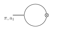
(a)

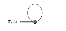
(b)

Figure 1: Diagrammatic representation of the contributions to the pion decay constant. The cross represents the axial current vertex.

The resulting one-loop contributions are diagrammatically schematized in Fig. 1. Tadpole-like diagrams, which are not present in the local NJL model, arise from the occurrence of gauge fields in Eqs. (29). We finally obtain

$$f_{\pi}=\dfrac{m_{c}\,g_{\pi q\bar{q}}}{m_{\pi}^{2}}\left[F_{0}(-m_{\pi}^{2})+\lambda(p^{2})\,F_{1}(-m_{\pi}^{2})\right]\ ,$$ (33)

where

$$F_{0}(p^{2}) = 8N_{c}\,\int\dfrac{d^{4}q}{(2\pi)^{4}}\,g(q)\,\dfrac{z(q^{+})z(q^{-})}{D(q^{+})D(q^{-})}\left[(q^{+}\cdot q^{-})+m(q^{+})\,m(q^{-})\right]\ ,$$

$$F_{1}(p^{2}) = 8N_{c}\,\int\dfrac{d^{4}q}{(2\pi)^{4}}\,h(q)\,\dfrac{z(q^{+})z(q^{-})}{D(q^{+})D(q^{-})}\left[(q^{+}\cdot p)\,m(q^{-})-(q^{-}\cdot p)\,m(q^{+})\right]\ .$$ (34)

It is important to notice that the result for $f_{\pi}$ does not depend on the path chosen for the transport function in Eq. (30) [see the comment after Eq. (42) below]. In the absence of vector meson fields, the mixing term in Eq. (33) vanishes and our expression reduces to that previously quoted in Ref. Noguera:2008 .

III.3 $\rho$ meson-photon vertex and $\rho$ electromagnetic decay constant

Another important quantity to be studied is the $\rho$-photon vertex. In our nonlocal model, meson-photon couplings receive in general contributions from the parallel transport in Eq. (29), therefore we find it important to check that the conservation of the vector current is satisfied. In addition, from this vertex we can obtain a prediction for the electromagnetic $\rho\to e^{+}e^{-}$ decay amplitude.

The $\rho$-photon vertex is given by the matrix element of the electromagnetic current between a vector meson state and the vacuum,

$$\langle 0|{\cal J}_{{\rm em}\,\mu}(x)|\tilde{v}_{\nu}^{a}(p)\rangle\ =\ i\,e^{-ip\cdot x}\,\Pi_{\mu\nu}^{a}(p)\ .$$ (35)

To calculate this matrix element one can follow the procedure discussed in the previous subsection, taking now

$${\cal G}_{\mu}\ =\ e\,Q\,{\mathcal{A}}_{\mu}\ ,$$ (36)

where $e$ is the proton charge and $Q={\rm diag}(2/3\;,\;-1/3)$.

Once again it is possible to distinguish two contributions to $\Pi_{\mu\nu}^{a}$, namely $\Pi_{\mu\nu}^{{\rm(I)}\,a}$ and $\Pi_{\mu\nu}^{{\rm(II)}\,a}$, arising from a two-vertex and a tadpole-like diagram, respectively (see Fig. 2). We obtain

$$\Pi_{\mu\nu}^{{\rm(I)}\,a}(p) = 4N_{C}\,\delta_{a3}\,e\,Z_{\rho}^{1/2}\int\dfrac{d^{4}q}{(2\pi)^{4}}\,\dfrac{z(q^{+})z(q^{-})}{D(q^{+})D(q^{-})}\;h(q)\;$$ (37)

$$\times\Bigg{\{}\frac{1}{2}\Big{[}\dfrac{1}{z(q^{+})}+\dfrac{1}{z(q^{-})}\Big{]}\Big{[}q^{+}_{\mu}\,q^{-}_{\nu}+q^{+}_{\nu}\,q^{-}_{\mu}-(q^{+}\cdot q^{-})\,\delta_{\mu\nu}-m(q^{+})m(q^{-})\,\delta_{\mu\nu}\Big{]}$$

$$+\;\bar{\sigma}_{1}\Big{[}m(q^{+})\,q^{-}_{\nu}+m(q^{-})\,q^{+}_{\nu}\Big{]}\;\alpha_{g\,\mu}(q,p)$$

$$+\;\bar{\sigma}_{2}\Big{[}-\frac{(q^{-})^{2}}{2}\,q_{\nu}^{+}-\frac{(q^{+})^{2}}{2}\,q_{\nu}^{-}+m(q^{+})m(q^{-})\,q_{\nu}\Big{]}\alpha_{f\,\mu}(q,p)\Bigg{\}}\ ,$$

$$\Pi_{\mu\nu}^{{\rm(II)}\,a}(p) = -\,4N_{C}\,\delta_{a3}\,e\,Z_{\rho}^{1/2}\int\dfrac{d^{4}q}{(2\pi)^{4}}\,\dfrac{z(q)}{D(q)}\ q_{\nu}\,\alpha_{h\,\mu}(q,p)\ .$$ (38)

Here we have defined, for a given function $f(p)$,

$$\alpha_{f\,\mu}(q,p)\ =\ \int\dfrac{d^{4}\ell}{(2\pi)^{4}}\;\Big{[}f(q+\ell/2)\,F_{\mu}(p-\ell,\ell)+f(q-\ell/2)\,F_{\mu}(\ell,p-\ell)\Big{]}\ ,$$ (39)

with

$$F_{\mu}(k,k^{\prime})\ =\ -\,i\int d^{4}z\;e^{ik^{\prime}z}\int_{0}^{z}ds_{\mu}\;e^{-i(k+k^{\prime})s}\ ,$$ (40)

where $s$ runs over a path connecting the origin with a point located at $z$.

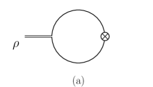
(a)

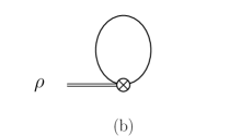
(b)

Figure 2: Diagrams contributing to the $\rho$ meson-photon vertex.

It can be seen that the tensors $\Pi_{\mu\nu}^{{\rm(I)}\,a}$ and $\Pi_{\mu\nu}^{{\rm(II)}\,a}$ are in general not transverse. However, the sum of both contributions satisfies $p^{\mu}\,\Pi_{\mu\nu}^{a}=0$, as required from the conservation of the electromagnetic current. This can be verified by noting that

$$(k+k^{\prime})^{\mu}F_{\mu}(k,k^{\prime})\ =\ -\,i\int d^{4}z\;e^{ik^{\prime}z}\int_{0}^{z(k+k^{\prime})}d\omega\;e^{-i\omega}\ =\ (2\pi)^{4}\Big{[}\delta^{(4)}(k)-\delta^{(4)}(k^{\prime})\Big{]}\ ,$$ (41)

which leads to

$$p^{\mu}\alpha_{f\,\mu}(q,p)\ =\ f(q^{+})-f(q^{-})\ .$$ (42)

It is also worth noticing that the integral in Eq. (41) becomes trivial, therefore the result in Eq. (42) does not depend on the integration path in Eq. (40) [a similar mechanism leads to the path independence of the functions in Eqs. (34)]. Using the relation in Eq. (42), after an adequate change of variables one obtains

$$p^{\mu}\Big{(}\Pi_{\mu\nu}^{{\rm(I)}\,a}+\Pi_{\mu\nu}^{{\rm(II)}\,a}\Big{)}\ =\ 0\ .$$ (43)

A similar cancellation has been found in Ref. Plant:1997jr , where a nlNJL model that includes vector mesons without quark WFR is considered.

Let us now concentrate on the $\rho$ electromagnetic decay constant $f_{v}$, which can be defined from $\rho^{0}\to e^{+}e^{-}$ decay:

$$\Gamma(\rho^{0}\to e^{+}e^{-})\ =\ \frac{4\pi}{3}\,\alpha^{2}\,m_{\rho}\,f_{v}^{2}\ ,$$ (44)

where $\alpha=e^{2}/(4\pi)$ is the electromagnetic fine structure constant. It can be seen that $f_{v}$ is related to the trace of $\Pi_{\mu\nu}^{3}(p)$ through

$$3\,m_{\rho}^{2}\,e\,f_{v}\ =\ g_{\mu\nu}\,\Pi_{\mu\nu}^{3}(p)\Big{|}_{p^{2}=-m_{\rho}^{2}}\ .$$ (45)

To evaluate the transverse part of the tensor $\Pi_{\mu\nu}^{3}$ we take a straight line path for the integral over $s_{\mu}$ in Eq. (30). This leads to

$$\alpha_{f\,\mu}(q,p)\ =\ \int^{1}_{-1}d\lambda\ \left(q_{\mu}+\lambda\dfrac{p_{\mu}}{2}\right)f^{\prime}\left(q+\lambda\dfrac{p}{2}\right)\ ,$$ (46)

where $f^{\prime}(p)$ denotes the derivative of $f$ with respect to $p^{2}$. After some algebra, we obtain

$$f_{v}\ =\ \dfrac{Z_{\rho}^{1/2}}{3\,m_{\rho}^{2}}\,\left[J^{\rm(I)}(-m_{\rho}^{2})+J^{\rm(II)}(-m_{\rho}^{2})\right]\ ,$$ (47)

where

$$J^{\rm(I)}(p^{2}) = -\,4N_{c}\,\int\dfrac{d^{4}q}{(2\pi)^{4}}\,h(q)\,\Bigg{\{}\dfrac{3}{2}\,\dfrac{[z(q^{+})+z(q^{-})]}{D(q^{+})D(q^{-})}\Big{[}(q^{+}\cdot q^{-})+m(q^{+})\,m(q^{-})\Big{]}$$

$$+\;\dfrac{1}{2}\,\dfrac{z(q^{+})}{D(q^{+})}\,+\,\dfrac{1}{2}\,\dfrac{z(q^{-})}{D(q^{-})}\,+\,\dfrac{q^{2}}{(q\cdot p)}\left[\dfrac{z(q^{+})}{D(q^{+})}-\dfrac{z(q^{-})}{D(q^{-})}\right]$$

$$+\,\dfrac{z(q^{+})z(q^{-})}{D(q^{+})D(q^{-})}\,\left[(q\cdot p)-\dfrac{q^{2}\,p^{2}}{(q\cdot p)}\right]\,\bigg{[}-\,\bar{\sigma}_{1}\,\big{[}m(q^{+})+m(q^{-})\big{]}\,\alpha^{+}_{g}(q,p)$$

$$+\;\bar{\sigma}_{2}\,\big{[}q^{2}+\dfrac{p^{2}}{4}-m(q^{+})\,m(q^{-})\big{]}\,\alpha^{+}_{f}(q,p)\,\bigg{]}\Bigg{\}}\ ,$$

$$J^{\rm(II)}(p^{2}) = -\,4N_{c}\int\dfrac{d^{4}q}{(2\pi)^{4}}\,\dfrac{z(q)}{D(q)}\left\{\dfrac{q^{2}}{(q\cdot p)}\Big{[}h(q^{+})-h(q^{-})\Big{]}+\left[(q\cdot p)-\dfrac{q^{2}\,p^{2}}{(q\cdot p)}\right]\alpha^{+}_{h}(q,p)\right\}.$$ (48)

Superindices (I) and (II) correspond to the contributions from the diagrams in Figs. 2a and 2b, respectively, while the functions $\alpha^{+}_{f}(q,p)$ have been defined as

$$\alpha^{\pm}_{f}(q,p)\ =\ \int_{-1}^{1}d\lambda\,\dfrac{\lambda}{2}\,f^{\prime}\left(q-\lambda\dfrac{p}{2}\right)\ .$$ (49)

III.4 $\pi^{0}\rightarrow\gamma\gamma$ decay

Let us analyze in the context of our model the anomalous decay $\pi^{0}\to\gamma\gamma$. As it is well known, in the NJL model this decay is problematic: in order to reproduce the experimentally observed result it is necessary to perform quark loop momentum integrations up to infinity instead of following the cutoff prescription of the model Blin:1987hw . In our framework, taking into account the discussion of gauge interactions in the previous subsections, the decay amplitude can be calculated from the matrix element

$$\langle 0|{\cal J}_{{\rm em}\,\mu}(x){\cal J}_{{\rm em}\,\nu}(0)|\tilde{\pi}^{3}(p)\rangle\ =\frac{\delta^{3}S_{E}^{\rm bos}}{\delta\mathcal{A}_{\mu}(x)\,\delta\mathcal{A}_{\nu}(0)\,\delta\tilde{\pi}^{3}(p)}\bigg{|}_{\mathcal{A}_{\mu,\nu}=\tilde{\pi}^{3}=0}\ .$$ (50)

In principle there are several diagrams that contribute to the amplitude at the level of one loop. As in the case of the pion decay constant $f_{\pi}$, since the physical $\pi^{0}$ state $\tilde{\pi}^{3}(p)$ is a combination of $\pi$ and $a_{\mu}$ fields, one has to consider the linear expansion of the bosonized action in $\pi$ and in $a_{\mu}$. The diagrams leading to nonzero contributions are those depicted in Fig. 3. If the outgoing photons are assumed to be in states of four-momenta $k_{1}$ and $k_{2}$ with polarization vectors $\varepsilon_{\mu}^{(\lambda_{1})}(k_{1})$ and $\varepsilon_{\nu}^{(\lambda_{2})}(k_{2})$, respectively, the decay amplitude can be written as

$${\cal M}(\pi^{0}\to\gamma\gamma)\ =\ i\,4\pi\alpha\,\tilde{F}(k_{1},k_{2})\,\epsilon^{\mu\nu\alpha\beta}\,\varepsilon_{\mu}^{(\lambda_{1})}(k_{1})^{\ast}\varepsilon_{\nu}^{(\lambda_{2})}(k_{2})^{\ast}k_{1\alpha}\,k_{2\beta}\ ,$$ (51)

where the form factor $\tilde{F}(k_{1},k_{2})$ is given by the sum of $\pi$ and $a_{\mu}$ contributions to the $\tilde{\pi}^{3}$ state,

$$\tilde{F}(k_{1},k_{2})\ =\ Z_{\pi}^{1/2}\,[F_{\pi}(k_{1},k_{2})\,+\,\lambda(p^{2})\,F_{a}(k_{1},k_{2})]\ ,$$ (52)

with $p=k_{1}+k_{2}$.

The first term in the brackets, corresponding to the diagram in Fig. 3a, has been calculated (apart from an isospin factor) in Ref. Dumm:2010hh . One has

$$F_{\pi}(k_{1},k_{2})\ =\ \frac{2N_{c}}{3}\,\int\dfrac{d^{4}q}{(2\pi)^{4}}\,h\bigg{(}q+\frac{k_{2}}{2}-\frac{k_{1}}{2}\bigg{)}\,\dfrac{z(q)z(q-k_{1})z(q+k_{2})}{D(q)D(q-k_{1})D(q+k_{2})}\,A(q,k_{1},k_{2})\ ,$$ (53)

where

$$A(q,k_{1},k_{2}) = \bigg{(}\frac{1}{z(q)}\,+\,\frac{1}{z(q-k_{1})}\bigg{)}\bigg{(}\frac{1}{z(q)}\,+\,\frac{1}{z(q+k_{2})}\bigg{)}\,\bigg{\{}m(q)\,-\,\frac{q^{2}}{2}\times$$ (54)

$$\left[\frac{m(q+k_{2})-m(q)}{(q\cdot k_{2})}\,-\,\frac{m(q-k_{1})-m(q)}{(q\cdot k_{1})}\right]\bigg{\}}\ .$$

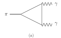
(a)

(b)

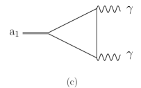
(c)

Figure 3: Diagrams contributing to $\pi^{0}\rightarrow\gamma\gamma$ decay.

On the other hand, the form factor $F_{a}(k_{1},k_{2})$ arises from the sum of the contributions corresponding to the diagrams in Figs. 3b and 3c. Although these turn out to be separately divergent, it is seen that divergent pieces cancel out and the sum is finite. We obtain

$$F_{a}(k_{1},k_{2}) = -\,\frac{2N_{c}}{3}\,\int\dfrac{d^{4}q}{(2\pi)^{4}}\;\Bigg{\{}h\big{(}q+k_{2}/2-k_{1}/2\big{)}\,\dfrac{z(q)z(q-k_{1})z(q+k_{2})}{D(q)D(q-k_{1})D(q+k_{2})}\times$$ (55)

$$\bigg{[}\Big{(}m(q-k_{1})+m(q+k_{2})\Big{)}\,A(q,k_{1},k_{2})\,+$$

$$\frac{q^{2}}{2}\bigg{(}\frac{B(q,q-k_{1},q+k_{2})}{(q\cdot k_{2})}\,-\,\frac{B(q,q+k_{2},q-k_{1})}{(q\cdot k_{1})}\bigg{)}\bigg{]}\,+$$

$$q^{2}\,\bigg{[}\frac{h(q+k_{2}/2)}{(q\cdot k_{2})}\,C(q,k_{1})\,+\,\frac{h(q+k_{1}/2)}{(q\cdot k_{1})}\,C(q,k_{2})\bigg{]}\Bigg{\}}\ ,$$

where

$$B(q,r,s) = \bigg{(}\frac{1}{z(q)}\,+\,\frac{1}{z(r)}\bigg{)}\bigg{(}\frac{1}{z(q)}\,-\,\frac{1}{z(s)}\bigg{)}\,D(s)\ ,$$

$$C(q,k) = \bigg{(}\frac{1}{z(q+k/2)}\,+\,\frac{1}{z(q-k/2)}\bigg{)}\,\frac{z(q+k/2)z(q-k/2)}{D(q+k/2)D(q-k/2)}\ .$$ (56)

Finally, after phase space integration and sum over outgoing photon polarizations, the $\pi^{0}\to\gamma\gamma$ decay amplitude is given by

$$\Gamma(\pi^{0}\to\gamma\gamma)\ =\ \frac{\pi}{4}\,\alpha^{2}\,m_{\pi}^{3}\,\tilde{F}(k_{1},k_{2})^{2}\ .$$ (57)

Since photons are on-shell, from Lorentz invariance it is seen that $\tilde{F}(k_{1},k_{2})$ can only be function of the scalar product $(k_{1}\cdot k_{2})=-m_{\pi}^{2}/2$.

III.5 $\rho\rightarrow\pi\pi$ decay

In general, various transition amplitudes can be calculated by expanding the bosonized action to higher orders in meson fluctuations. In this subsection we concentrate in the processes $\rho^{0}\to\pi^{+}\pi^{-}$ and $\rho^{\pm}\to\pi^{\pm}\pi^{0}$, which are responsible for more than 99% of $\rho$ meson decays. The decay amplitudes ${\mathcal{M}}(v^{a}(p)\to\pi^{b}(q_{1})\pi^{c}(q_{2}))$ are obtained by calculating the corresponding functional derivatives of the effective action, which can be written in terms of two form factors $\tilde{F}_{\rho\pi\pi}(p^{2},q_{1}^{2},q_{2}^{2})$ and $\tilde{G}_{\rho\pi\pi}(p^{2},q_{1}^{2},q_{2}^{2})$:

$$\frac{\delta^{3}S_{E}^{\rm bos}}{\delta\tilde{v}_{\mu}^{a}(p)\delta\tilde{\pi}^{b}(q_{1})\delta\tilde{\pi}^{c}(q_{2})}\bigg{|}_{\delta v_{\mu}=\delta\pi=0} = (2\pi)^{4}\ \delta^{(4)}(p+q_{1}+q_{2})\ \epsilon_{abc}\left[\tilde{F}_{\rho\pi\pi}(p^{2},q_{1}^{2},q_{2}^{2})\;\frac{(q_{1\mu}+q_{2\mu})}{2}\right.$$ (58)

$$\;+\;\left.\tilde{G}_{\rho\pi\pi}(p^{2},q_{1}^{2},q_{2}^{2})\;\frac{(q_{1\mu}-q_{2\mu})}{2}\right]\ .$$

Only the transverse piece, driven by the form factor $\tilde{G}_{\rho\pi\pi}(p^{2},q_{1}^{2},q_{2}^{2})$, contributes to $\rho\to\pi\pi$ decay widths. Indeed, in the isospin limit, one has

$$\Gamma_{\rho^{0}\to\pi^{+}\pi^{-}}\ =\ \Gamma_{\rho^{\pm}\to\pi^{\pm}\pi^{0}}\ =\ \frac{1}{48\pi}\;m_{\rho}\;g_{\rho\pi\pi}^{2}\left(1-\frac{4m_{\pi}^{2}}{m_{\rho}^{2}}\right)^{3/2}\ ,$$ (59)

where $g_{\rho\pi\pi}\equiv\tilde{G}_{\rho\pi\pi}(-m_{\rho}^{2},-m_{\pi}^{2},-m_{\pi}^{2})$.

The form factor $\tilde{G}_{\rho\pi\pi}(p^{2},q_{1}^{2},q_{2}^{2})$ arises from the effective vertex $\tilde{\rho}\tilde{\pi}\tilde{\pi}$, where $\tilde{\rho}$ and $\tilde{\pi}$ are renormalized states. Since we expand the effective action in Eq. (4) in powers of the unrenormalized fields, it is convenient to write the effective vertex in terms of the original fields $\rho$, $\pi$ and $a_{\mu}$ [the latter has to be taken into account due to the $\pi-a$ mixing given by Eq. (23), as mentioned in previous subsections]. In this way, the form factor receives contributions from the diagrams sketched in Fig. 4. One has

$$\tilde{G}_{\rho\pi\pi}(p^{2},q_{1}^{2},q_{2}^{2}) = Z_{\rho}^{1/2}\,Z_{\pi}\,\bigg{[}G_{\rho\pi\pi}(p^{2},q_{1}^{2},q_{2}^{2})+$$ (60)

$$\lambda(p^{2})\ G_{\rho\pi a}(p^{2},q_{1}^{2},q_{2}^{2})+\lambda(p^{2})^{2}\ G_{\rho aa}(p^{2},q_{1}^{2},q_{2}^{2})\bigg{]}\ ,$$

where $G_{\rho\pi\pi}(p^{2},q_{1}^{2},q_{2}^{2})$, $G_{\rho\pi a}(p^{2},q_{1}^{2},q_{2}^{2})$ and $G_{\rho aa}(p^{2},q_{1}^{2},q_{2}^{2})$ are one-loop functions that arise from the expansion of the effective action. The explicit forms of these functions, which can be obtained after a rather lengthy calculation, can be found in Appendix A.

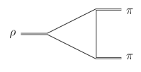
(a)

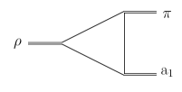
(b)

(c)

Figure 4: Diagrams contributing to $\rho\rightarrow\pi\pi$ decays.

IV Numerical results

IV.1 Model parameters and form factors

To fully define the model it is necessary to provide the values of the unknown parameters and to specify the shape of the form factors entering the nonlocal fermion currents. There are six parameters, namely, the current quark mass $m_{c}$ and the dimensionful coupling constants $G_{S}$, $G_{V}$, $G_{0}$, $G_{5}$ and $\varkappa$. Regarding the form factors, as stated in the Introduction, we will take into account the results obtained in lattice QCD for the momentum dependence of the mass and WFR in the quark propagator. Therefore, following Ref. Bowman:2002bm , we write the effective mass $m(p)$ as

$$m(p)\ =\ m_{c}\,+\,\alpha_{m}\,f_{m}(p^{2})\ ,$$ (61)

where $\alpha_{m}$ is a mass parameter defined by the normalization condition $f_{m}(0)=1$. Since LQCD calculations involve various current quark masses, we have chosen to take as input the shape of the (normalized) function $f_{m}(p^{2})$, taking LQCD results in the limit of low $m_{c}$ and smallest lattice spacing. Considering the LQCD analysis in Ref. Bowman:2002bm , we parameterize this function by

$$f_{m}(p^{2})\ =\ \frac{1}{1+(p^{2}/\Lambda_{0}^{2})^{\alpha}}\ ,$$ (62)

with $\alpha=3/2$. On the other hand, for the wave function renormalization we use the parametrization Noguera:2005ej ; Noguera:2008

$$z(p)\ =\ 1\,-\,\alpha_{z}\,f_{z}(p^{2})\ ,$$ (63)

where

$$f_{z}(p^{2})\ =\ \frac{1}{\left(1+p^{2}/\Lambda_{1}^{2}\right)^{\beta}}\ .$$ (64)

It is found that LQCD results favor a relatively low value for the exponent $\beta$, therefore we take here $\beta=5/2$, which is the smallest exponent compatible with the ultraviolet convergence of the gap equations (12). As required by dimensional analysis and Lorentz invariance, the functions $f_{m}(p^{2})$ and $f_{z}(p^{2})$ carry dimensionful parameters $\Lambda_{0}$ and $\Lambda_{1}$, which represent effective cutoff momenta in the corresponding channels. Thus, we will use here the above functional forms for the form factors, taking $\Lambda_{0}$ and $\Lambda_{1}$ as two further free parameters of the model. Regarding the parameters $\alpha_{m}$ and $\alpha_{z}$ introduced in Eqs. (61) and (63), from Eqs. (11) it is seen that they are related to the mean field values of the scalar fields by

$$m(0) = m_{c}+\alpha_{m}\ =\ \frac{m_{c}+\bar{\sigma}_{1}}{1-\bar{\sigma}_{2}}\ ,$$ (65)

$$z(0) = 1-\alpha_{z}\ =\ \frac{1}{1-\bar{\sigma}_{2}}\ ,$$ (66)

hence, for a given set of model parameters, they can be obtained by solving the gap equations (12).

The model also includes the form factors $h(p)$, $h_{0}(p)$ and $h_{5}(p)$, introduced through the vector and axial vector current-current interactions. For definiteness and simplicity we will assume the effective behavior of quark interactions to be similar in the $J=0$ and $J=1$ channels, therefore we will take for $h(p)$ the same form as $g(p)$. Regarding the vector-isoscalar sector, as it is usually done we assume approximate degeneracy with the vector-isovector part, hence we take $h(p)\simeq h_{0}(p)$. The axial vector-isoscalar sector can be studied separately, since it decouples from the rest of the Lagrangian. Here we will just take $h_{5}(p)=h(p)$ in order to get an estimation for the constant $G_{5}$ from phenomenology.

Given the form factor shapes, in order to study the phenomenology we have to determine the values of the model parameters (current quark mass, coupling constants and effective cutoff momenta). To do this, we first carry out a fit to lattice results for the functions $f_{m}(p^{2})$ and $z(p)$, from which we obtain the values of the cutoffs $\Lambda_{0}$ and $\Lambda_{1}$, as well as the parameter $\alpha_{z}$. The latter will be used, together with five phenomenological quantities, as input to determine the remaining six free model parameters. From the LQCD results quoted in Ref. Parappilly:2005ei we obtain

$$\Lambda_{0}=917\,\pm\,14\,{\rm\ MeV}\ ,\qquad\Lambda_{1}=1775\,\pm\,53\,{\rm\ MeV}\ ,\qquad\alpha_{z}=0.244\,\pm\,0.010\,\ ,$$ (67)

with $\chi^{2}/{\rm dof}=1.17$ and $\chi^{2}/{\rm dof}=0.25$ for the fits to $f_{m}(p^{2})$ and $z(p)$ data, respectively. The fits have been carried out considering lattice values up to 2.5 GeV. Both the data and the fitting curves for $f_{m}(p^{2})$ and $z(p)$ are shown in Fig. 5. In the case of $z(p)$, it is seen that the fit leads to somewhat large values of $z(p)$ at low momenta in comparison with lattice points. We notice, however, that errors in this region are relatively large, and in addition these points are the most sensitive to changes in lattice spacing and/or sea quark masses Parappilly:2005ei .

Figure 5: Fit to lattice data for the functions $f_{m}(p^{2})$ and $z(p)$.

Once the form factor shapes have been fixed, one can set the model parameters so as to reproduce the empirical values of some selected observables. As stated, we take from the fit the values of $\Lambda_{0}$ and $\Lambda_{1}$ and then we determine the values of the parameters $m_{c}$, $G_{V}$, $G_{S}$, $G_{0}$, $G_{5}$ and $\varkappa$ from six input quantities. These have been chosen to be the fitted value of $\alpha_{z}$ together with the empirical values of the pion weak decay constant $f_{\pi}$ and the masses of the $\pi$, $\rho$, $\omega$ and $f_{1}$ mesons. From our numerical analysis we find that there is a set of parameters that allows us to properly reproduce these empirical values. The corresponding results are quoted in Table I.

Model parameters	Inputs	Model parameters		Inputs
$\Lambda_{0}$ [MeV]	LQCD results	$m_{c}$ [MeV]	1.59	$\alpha_{z}$	LQCD results
$\Lambda_{1}$ [MeV]	LQCD results	$G_{S}\Lambda_{0}^{2}$	19.0	$m_{\pi}$ [MeV]	139
		$\varkappa/\Lambda_{0}$	11.2	$f_{\pi}$ [MeV]	92.2
		$G_{V}\Lambda_{0}^{2}$	13.0	$m_{\rho}$ [MeV]	775
		$G_{0}\Lambda_{0}^{2}$	12.8	$m_{f_{1}}$ [MeV]	1280
		$G_{5}\Lambda_{0}^{2}$	$\sim 14$	$m_{\omega}$ [MeV]	783

Table 1: Model parameters. The values of $\Lambda_{0}$, $\Lambda_{1}$ and $\alpha_{z}$ have been obtained from a fit to lattice QCD calculations for the effective quark propagator, see Eq. (67). The model parameters $m_{c}$, $G_{S}$, $\varkappa$, $G_{V}$, $G_{0}$ and $G_{5}$ are fitted against the phenomenological values of five hadronic observables, plus the value of $\alpha_{z}$ given by the fit to LQCD data.

The numerical analysis requires solving a system of coupled equations that includes the gap Eqs. (12), equations $G_{M}(-m_{M}^{2})=0$ for $M=\pi,\rho,\omega$ and $f_{1}$ to determine meson masses, and Eq. (33) for $f_{\pi}$. This involves the calculation of one-loop integrals introduced in Secs. III.A and III.B, which in general is not a trivial task due to the fact that the form factor $f_{m}(p^{2})$, as function of the fourth component $p_{4}$ of the momentum, has cuts when $p_{4}$ is extended to the complex plane. Depending on the value of the three-momentum $\vec{p}$ these cuts can occasionally cross the real axis, and have to be taken into account through a proper deformation of the integration path. Details of the calculations are given in Appendix B.

From Table I we find a ratio $G_{S}/G_{V}\sim 1.5$, which is in agreement with standard NJL model parametrizations njlrev . Concerning the value of $G_{0}$, it is necessary to take into account that we are working within a two-flavor model, therefore effects of strange quark bound states are not explicitly considered. Our determination of $G_{0}$ would be valid only in the case of “ideal mixing” between SU(3)_f singlet and octet $I=0$ states, which means taking the $\omega$ as an approximate SU(3)_f octet state, and the $\phi$ meson as an approximately pure $\bar{s}s$ state. In the case of the $f_{1}$ axial vector meson there is an additional problem, which is common to various quark models. Indeed, models that do not include an explicit mechanism of confinement usually have difficulties for describing meson resonances, since there is a threshold above which the meson mass becomes large enough to allow the decay of the meson into two quarks. This threshold is typically of the order of $2m(0)$, therefore models that lead to constituent masses larger than about 400 MeV (as occurs in our case) can avoid this problem for low mass resonances like the $\rho$ meson He:1997gn . Other possible approaches are e.g. the extension of $G_{M}(-s)$ functions to the complex plane Zhuang:1994dw or the search for a peak in the meson spectral function Hansen:2006ee . Mathematically, in our model the onset of the unphysical $q\bar{q}$ channel corresponds to the fact that in the integrals of the form of e.g. Eq. (17) there is a “pinch point” at which both functions $D(q^{+})$ and $D(q^{-})$ in the integrand are equal to zero (i.e. both constituent quarks are simultaneously on shell). For the parameters in Table I, the threshold is found to be at 1264 MeV, i.e. below the empirical value $m_{f_{1}}=1280$ MeV, and the free parameter to be adjusted to get the phenomenological value of the $f_{1}$ mass is the coupling constant $G_{5}$. To obtain an approximate value for this constant, we have solved the equation $G_{f_{1}}(-m^{2})=0$ varying $G_{5}\Lambda_{0}^{2}$ from large values of $G_{5}$ up to $G_{5}\Lambda_{0}^{2}\simeq 22$, which leads to $m\simeq 1$ GeV, and then we have extrapolated to the region above the threshold to obtain $m_{f_{1}}\simeq 1280$ MeV for $G_{5}\Lambda_{0}^{2}\sim 14$.

IV.2 Numerical results for phenomenological quantities

Using the parameters and nonlocal form factors quoted in the previous subsection, we can calculate the predictions of the model for the phenomenological quantities analyzed in Secs. II and III.

Our numerical results for various observables are summarized in Table II (we have not included here the quantities taken as phenomenological inputs, namely $m_{\pi}$, $f_{\pi}$, $m_{\rho}$, $m_{\omega}$ and $m_{f_{1}}$). From the table it is seen that the predictions of the model for the $\pi^{0}\to\gamma\gamma$, $\rho\to e^{+}e^{-}$ and $\rho\to\pi\pi$ decay rates are in good agreement with experiments, being compatible with the empirical values pdg within an accuracy of less than 10%. We can also obtain a prediction for the width $\Gamma(\omega\to e^{+}e^{-})$, which is found to be about 0.8 keV, somewhat larger than the experimental value $0.60\pm 0.02$ keV pdg . However, as discussed above, our result might become modified after the inclusion of strangeness degrees of freedom owing to the $\omega-\phi$ mixing. Regarding the $\sigma-\sigma^{\prime}$ sector, we obtain a physical state with a mass of about 680 MeV, which can be identified with the observed $\sigma$ meson resonance (the mass of which is rather uncertain), while for the state $\sigma^{\prime}$ we find that the function $G_{\sigma^{\prime}}(-s)$ grows monotonically with $s$, indicating that this state does not represent a physical meson (a more detailed discussion on the $\sigma^{\prime}$ state in this type of models can be found in Ref. Noguera:2008 ). In the case of the a₁ vector mesons we find that the function $G_{{\rm a}_{1}}(-s)$ decreases with $s$ until it reaches a minimum at $\sqrt{s}\simeq 1250$ MeV, very close to the threshold of on-shell quark pair production, or pinch point, found at 1264 MeV. Recalling the discussion in the previous subsection, in order to estimate the value of the ${{\rm a}_{1}}$ mass it is possible either to take the minimum of $G_{{\rm a}_{1}}(-s)$ or to make an extrapolation based on the behavior of $G_{{\rm a}_{1}}(-s)$ up to say $s\sim(1\ {\rm GeV})^{2}$. Both approaches lead to $m_{{\rm a}_{1}}\sim 1200-1250$ MeV, which is in good agreement with experimental expectations. We have also analyzed the dependence of our results on the value of $\alpha_{z}$ within the error given by the fit to LQCD data [see Eq. (67)], obtaining that the model predictions do not vary significantly.

		Model	Empirical
	$\Gamma(\pi^{0}\to\gamma\gamma)$ [MeV]	$7.82\times 10^{-6}$	$(7.63\pm 0.16)\times 10^{-6}$
	$\Gamma(\rho\to e^{+}e^{-})$ [MeV]	$6.71\times 10^{-3}$	$(7.04\pm 0.06)\times 10^{-3}$
	$\Gamma(\rho\to\pi\pi)$ [MeV]	137	$149.1\pm 0.8$
	$m_{\sigma}$ [MeV]	683	400 - 550
	$m_{{\rm a}_{1}}$ [MeV]	1200 - 1250	1190 - 1270

Table 2: Model predictions and empirical values pdg for various observables.

Finally, in Table III we quote our results for mean field values of scalar fields, chiral quark condensates and effective quark-meson couplings. It is seen that the model leads to a zero-momentum effective quark mass $m(0)=(m_{c}+\bar{\sigma}_{1})/(1-\bar{\sigma}_{2})\simeq 400$ MeV, somewhat larger than the value of 311 MeV obtained in Ref. Noguera:2008 for a nlNJL model without vector meson degrees of freedom. For comparison, notice that standard NJL model parametrizations lead to values of constituent (momentum-independent) quark masses around 350 MeV njlrev . Concerning the chiral quark condensates, our results are relatively large in comparison with usual phenomenological estimations and lattice calculations, which lead to condensates in the range of $(-240\ \rm{MeV})^{3}$ to $(-320\ \rm{MeV})^{3}$ McNeile:2005pd . In addition, when determining the model parameters we have found a relatively low value for the current quark mass, namely $m_{c}=1.59$ MeV, in comparison with lattice estimates that lead to $m_{c}\simeq 3.4\pm 0.25$ MeV in the isospin limit pdg . The results for these quantities in nlNJL models are in fact strongly dependent on the form factor shapes, as it is found in Refs. Noguera:2008 ; Carlomagno:2013ona ; Hell:2011ic , where two- and three-flavor nonlocal models (which do not include the vector meson sector) are considered. As discussed in those articles, one has to take into account that both $m_{c}$ and $\langle\bar{q}q\rangle$ are scale-dependent quantities, and our fit has been carried out using lattice data that correspond to a renormalization scale $\mu=3$ GeV, somewhat larger than the usual scale of 2 GeV. To get rid of the scale dependence one can look at the product $-\langle\bar{q}q\rangle m_{c}$, for which we get, within our parametrization, a result of about $8.12\times 10^{-5}$ GeV⁴. This is in good agreement with the value arising from the Gell-Mann-Oakes-Renner relation at the leading order in the chiral expansion, namely $-\langle\bar{q}q\rangle m_{c}=f^{2}_{\pi}m_{\pi}^{2}/2\simeq 8.21\times 10^{-5}$ GeV⁴. Finally, for completeness we include in Table III the values obtained for the effective quark-meson couplings $g_{\pi q\bar{q}}$ and $g_{\rho q\bar{q}}$.

		Model
	$\bar{\sigma}_{1}$ [MeV]	524
	$\bar{\sigma}_{2}$	-0.322
	$-\langle\bar{q}q\rangle^{1/3}$ [MeV]	371
	$g_{\pi q\bar{q}}$	5.69
	$g_{\rho q\bar{q}}$	2.94

Table 3: Numerical results for various phenomenological quantities.

V Summary & outlook

In this work we have introduced a two-flavor chiral quark model that includes nonlocal four-fermion interactions. Besides the usual scalar and pseudoscalar couplings already present in the standard (local) NJL model, we consider the couplings between vector and axial-vector quark-antiquark currents as well as a current-current interaction that leads to WFR of the quarks fields. The model leads to a dressed quark propagator in which the effective mass and WFR are functions of the momentum through nonlocal form factors, and these can be fitted to the results obtained in lattice QCD calculations.

We have concentrated on vacuum properties related with the presence of vector and axial-vector mesons, which have not been taken into account in this context in previous works. For this analysis we have evaluated various one-loop diagrams contributing to vector and axial-vector mass terms and decay amplitudes. It is seen that, owing to the nonlocal character of the interactions, the model leads to tadpole diagrams contributing to the $\rho-$photon vertex, in addition to the usual quark loop contributions. The longitudinal components of both contributions are found to be separately nonvanishing, while their sum is transverse, as requested by electromagnetic current conservation. It is worth mentioning that analytical expressions for the pion mass and decay constants obtained in previous works have been revisited in order to take into account $\pi-$a₁ mixing.

On the phenomenological side, the fit of nonlocal form factors to lattice QCD results for effective quark propagators provides a more natural and realistic way to regularize the model in comparison with the standard NJL approach. The remaining unknown parameters, namely the current quark mass and the current-current coupling constants, can be determined from some input observables. Here we have chosen to take as inputs the measured values of the pion decay constant and a set of meson masses. From the numerical evaluation of the analytical expressions we find that the model is able to properly reproduce the empirical values of these observables, and leads to phenomenologically acceptable values for other scalar and vector meson masses and decay widths.

To conclude, let us state that the inclusion of the axial and vector meson sector offers a more complete picture of hadron phenomenology in the framework of nonlocal quark models, and its effects can be important for the analysis of hadronic observables such as the pion electromagnetic form factor and the vector and axial vector form factors for pion radiative decays. It is also worth it to extend the study of $\rho$ meson properties to finite-temperature systems, given its importance for the study of heavy ion collisions. In addition, for the case of hadronic systems at finite chemical potential it is expected that vector interactions lead to a nonzero condensate in the $J=1$, $I=0$ channel, which can be important for the study of the QCD phase diagram Hell:2012da and the physics of compact objects Blaschke:2007ri . We expect to report on these issues in forthcoming articles.

Appendix A: Analytical expressions for the form factors in $\rho\to\pi\pi$ decays

Here we quote the analytical expressions for the functions $G_{\rho\pi\pi}(p^{2},q_{1}^{2},q_{2}^{2})$, $G_{\rho\pi a}(p^{2},q_{1}^{2},q_{2}^{2})$ and $G_{\rho aa}(p^{2},q_{1}^{2},q_{2}^{2})$ contributing to the form factor $\tilde{G}_{\rho\pi\pi}(p^{2},q_{1}^{2},q_{2}^{2})$, see Eq. (60). To calculate the $\rho\to\pi\pi$ decay amplitude, we have to evaluate these functions at $q_{1}^{2}=q_{2}^{2}=(p-q_{1})^{2}=-m_{\pi}^{2}$, $p^{2}=-m_{\rho}^{2}$. We find it convenient to introduce the momentum $v=q_{1}-p/2$, which satisfies $p\cdot v=0$, $v^{2}=m_{\rho}^{2}/4-m_{\pi}^{2}$. Then the functions $G_{\rho xy}(p^{2},q_{1}^{2},q_{2}^{2})$, where subindices $x$ and $y$ stand for either $\pi$ or $a$, can be written as

$$G_{\rho xy}(p^{2},q_{1}^{2},q_{2}^{2}) = 16N_{c}\,\int\dfrac{d^{4}q}{(2\pi)^{4}}\,h(q)\,g\left(q+v/2+p/4\right)\,g\left(q+v/2-p/4\right)$$ (68)

$$\times\ \dfrac{z(q^{+})z(q^{-})z(q+v)}{D(q^{+})D(q^{-})D(q+v)}\;f_{xy}(q,p,v)\ ,$$

where we have defined $q^{\pm}=q\pm p/2$. After a rather lengthy calculation we find for $f_{xy}(q,p,v)$ the expressions

$$f_{\pi\pi} = \bigg{[}(q^{+}\cdot q^{-})+m(q^{+})\,m(q^{-})\bigg{]}\,\bigg{[}1+\dfrac{(q\cdot v)}{v^{2}}\bigg{]}$$

$$-\,\dfrac{(q\cdot v)}{v^{2}}\bigg{\{}2\,\Big{[}\,q\cdot(q+v)\Big{]}\,+\,m(q+v)\,\Big{[}m(q^{+})+\,m(q^{-})\Big{]}\bigg{\}}\ ,$$

$$f_{\pi a} = -2\,m(q+v)\left[(q^{+}\cdot q^{-})\,-\,2\,\dfrac{(q\cdot v)^{2}}{v^{2}}\,+\,m(q^{+})m(q^{-})\right]$$

$$+\,\bigg{[}1+\dfrac{(q\cdot v)}{v^{2}}\bigg{]}\,\bigg{\{}(q^{+}\cdot p)\,m(q^{-})-(q^{-}\cdot p)\,m(q^{+})\,-\,2(q\cdot v)\Big{[}m(q^{+})+m(q^{-})\Big{]}\bigg{\}}\ ,$$

$$f_{aa} = \bigg{[}1+\dfrac{(q\cdot v)}{v^{2}}\bigg{]}\bigg{[}q^{+2}\,q^{-2}\,-\,(q^{+}\cdot q^{-})\,(q+v)^{2}\,-\,\Big{(}v^{2}+\dfrac{p^{2}}{4}\Big{)}m(q^{+})m(q^{-})\bigg{]}$$ (69)

$$+\;m(q+v)\bigg{\{}m(q^{+})\,(q^{-}\cdot p)\,-\,m(q^{-})\,(q^{+}\cdot p)\,+\,\dfrac{(q\cdot v)}{v^{2}}\bigg{(}v^{2}-\dfrac{p^{2}}{4}\bigg{)}\,\Big{[}m(q^{+})\,+\,m(q^{-})\Big{]}\bigg{\}}$$

$$+\;2\,\dfrac{(q\cdot v)}{v^{2}}\,(q+v)^{2}\bigg{[}(q\cdot v)-\dfrac{p^{2}}{4}\bigg{]}\ .$$

Appendix B: Loop integrals and branch cuts in the form factors

As described in Sec. IV, we have considered a parametrization of the nlNJL model that allows us to reproduce LQCD results for the momentum dependence of effective quark propagators. From the comparison with LQCD data, the form factors $g(p)$ and $f(p)$ have been written in terms of the functions $f_{m}(p^{2})$ and $f_{z}(p^{2})$ given by Eqs. (62) and (64). In this appendix we discuss the numerical evaluation of loop integrals, which have to be treated with some care given the particular form of $f_{m}(p^{2})$.

Let us consider loop integrals that involve an external momentum $p$, such as those in the functions $G_{M}(p^{2})$, $F_{0,1}(p^{2})$ and $J^{({\rm I},{\rm II})}(p^{2})$, defined in Sec. III. The integrals can be generically written as

$$I(p^{2})\ =\ \int\dfrac{d^{4}q}{(2\pi)^{4}}\;F(q^{+},q^{-},p)\ ,$$ (70)

where $q^{\pm}=q\pm p/2$, and $F(q^{+},q^{-},p)$ is a function that includes the form factors either explicitly or through the quark effective masses and/or wave function renormalizations. More precisely, it is seen that in general $F(q^{+},q^{-},p)$ may include the form factors $f_{m}(s)$ evaluated at $s=(q^{+})^{2}$, $(q^{-})^{2}$ and/or $q^{2}$. We are interested in this form factor since its explicit form $f_{m}(s)=1/[1+(s/\Lambda_{0}^{2})^{3/2}]$ implies the existence of a branch cut in the complex plane $s$, namely at Re$(s)<0$, Im$(s)=0$. It is worth noticing that in all cases the integrals have to be evaluated numerically at $p^{2}=-M^{2}$, where $M$ is some meson mass.

To perform the calculations we choose, as usual, the 4th axis in the direction of the external momentum. Thus one has $p^{\mu}=(iM,\vec{0})$, and $I(p^{2})$ can be reduced to a double integral in $q_{4}$ and $|\vec{q}|$. Since the functions $F(q^{+},q^{-},p)$ are symmetric under the exchange $q^{+}\leftrightarrow q^{-}$, it is easy to see that $F(q^{+},q^{-},p)=F({q^{+}}^{\ast},{q^{-}}^{\ast},p)$, which ensures the reality of $I(q^{2})$. Now let us take $|\vec{q}|$ fixed, and consider the analytical structure of the integrand in the complex $q_{4}$ plane. It is immediately seen that we will find a pair of branch cuts in this plane arising from the function $f_{m}(q^{2})$, and other pairs of cuts will appear from the occurrences of $f_{m}[(q^{+})^{2}]$ and $f_{m}[(q^{-})^{2}]$, respectively. In the case of $f_{m}(q^{2})=f_{m}(q_{4}^{2}+|\vec{q}|^{2})$, the cuts are given by Re$(q_{4})=0$, $|{\rm Im}(q_{4})|>|\vec{q}|$, hence they never cross the real $q_{4}$ axis, along which the integral is to be performed. On the other hand, for $f_{m}[(q^{\pm})^{2}]$ the cuts are located at Re$(q_{4})=0$, $|{\rm Im}(q_{4})\pm M/2|>|\vec{q}|$, therefore if $|\vec{q}|<M/2$, both $f_{m}[(q^{+})^{2}]$ and $f_{m}[(q^{-})^{2}]$ have cuts that cross the real $q_{4}$ axis.

The treatment of these cuts is a matter of prescription. In fact, after taking the form factors from LQCD calculations in Euclidean space, one could turn back to Minkowski space through a Wick rotation. Then one would find that the cuts are located along the integration axis, and to evaluate the integrals they have to be moved away according to some recipe. Here we will adopt the prescription of translating the arguments of $f_{m}(s)$ according to

$$f_{m}[(q^{+})^{2}] \rightarrow f_{m}[(q^{+})^{2}-i\varepsilon]\ ,$$ (71)

$$f_{m}[(q^{-})^{2}] \rightarrow f_{m}[(q^{-})^{2}+i\varepsilon]\ ,$$ (72)

while $f_{m}(q^{2})$ is kept unchanged. In this way, branch cuts do not overlap and the property $F(q^{+},q^{-},p)=F({q^{+}}^{\ast},{q^{-}}^{\ast},p)$ remains valid. From Eqs. (71) and (72) the cuts associated to the functions $f_{m}[(q^{\pm})^{2}]$ are given by

$$\left\{\begin{array}[]{rcl}{\rm Re}(q_{4})-\dfrac{\varepsilon}{M\pm 2\,{\rm Im}(q_{4})}&=&0\ \ ,\\ \hskip 14.22636pt\rule{0.0pt}{19.91684pt}|{\rm Im}(q_{4})\pm M/2|-|\vec{q}|&>&0\ \ .\end{array}\right.$$ (73)

The corresponding curves in the complex plane $q_{4}$ are sketched in Fig. 6, where we have distinguished two situations in which $|\vec{q}|>M/2$ (Fig. 6a) and $|\vec{q}|<M/2$ (Fig. 6b). Branch cuts corresponding to the functions $f_{m}[(q^{+})^{2}]$, $f_{m}[(q^{-})^{2}]$ and $f_{m}(q^{2})$ have been represented with dashed, dotted and dashed-dotted lines, respectively. If $|\vec{q}|>M/2$, as it is shown in Fig. 6a, the cuts do not cross the integration axis, thus there is no extra contribution to the loop integral. On the contrary, for $|\vec{q}|<M/2$ two branch cuts cross from one half-plane to the other one, passing through the real $q_{4}$ axis. Since the integral over $q_{4}$ has to be ultimately equivalent to an integral over the Minkowski momentum $q_{0}$, obtained through the corresponding Wick rotation, the integration contour along $q_{4}$ should be deformed in order to subtract the contribution of the crossing pieces, which are represented with solid lines in Fig. 6b. A similar procedure has to be followed when poles of the integrand cross the integration axis at some value of $|\vec{q}|$; in that case the contributions resulting from the deformation of the $q_{4}$ integration contour can be obtained by calculating the residues of the poles, according to Cauchy’s theorem. The need to add cut or pole contributions to the loop integrals becomes evident by looking at relatively simple integrals as those appearing in the gap equations (12): if one carries out a translation of the loop momentum $p\to p\,^{\prime}=p+r$, with $r^{2}=-M^{2}$, for fixed $|\vec{p}\,^{\prime}|$ there will be branch cuts in the complex plane $p\,^{\prime}_{4}$ that cross from the upper half-plane to the lower one (or vice versa). In addition, in general the integrand will have poles that for large enough values of $M$ cross the real $p\,^{\prime}_{4}$ axis at some value of $|\vec{p}\,^{\prime}|$. From Cauchy’s theorem it is easy to see that the corresponding contributions have to be subtracted if one requires the loop integral to be invariant under the translation.

(a)

Figure 6: Branch cuts of the functions $F(q^{+},q^{-},p)$ in the complex plane $q_{4}$, according to the prescription in Eqs. (71) and (72). The curves in graphs (a) and (b) correspond to $|\vec{q}|>M/2$ and $|\vec{q}|<M/2$, respectively.

In practice the contributions from the cuts can be obtained by carrying out integrations in the $q_{4}$ plane along adequate contours that enclose the crossing pieces, letting then $\varepsilon\to 0$. Owing to the symmetry of the functions $F(q^{+},q^{-},p)$ imaginary parts from the integrations in the upper and lower half-planes cancel out, leading to a real total contribution. Then the result has to be integrated over the three-momentum variable $|\vec{q}|$. Notice that —according to the conditions in Eq. (73)— this integration goes from $|\vec{q}|=0$ to $|\vec{q}|=M/2$, therefore the contribution can be neglected if the meson mass $M$ is relatively small, which is in general the case when $M=m_{\pi}$. Finally, in the case of the $\rho\to\pi\pi$ form factor the situation is more complicated since the relevant loop integral, given by Eq. (68), involves two independent external momenta $p$ and $v$. It can be seen that the integrand has two additional branch cuts in the $q_{4}$ complex plane, arising from the functions $f_{m}(s)$ evaluated at $s=(q+v/2\pm p/4)^{2}$. To deal with these new cuts we have used the prescription $f_{m}[(q+v/2\pm p/4)^{2}]\rightarrow f_{m}[(q+v/2\pm p/4)^{2}\pm i\varepsilon^{\prime}]$, choosing an integration path that encloses the pieces of the cuts that cross the real $p_{4}$ axis as explained above.

References

- (1) Y. Nambu and G. Jona-Lasinio, Phys. Rev. 122, 345 (1961); 124 246 (1961).
- (2) U. Vogl and W. Weise, Prog. Part. Nucl. Phys. 27 195 (1991); S.P. Klevansky, Rev. Mod. Phys. 64 649 (1992); T. Hatsuda and T. Kunihiro, Phys. Rept. 247 221 (1994).
- (3) G. Ripka, Quarks Bound by Chiral Fields, (Oxford University, New York, 1997).
- (4) M. B. Parappilly, P. O. Bowman, U. M. Heller, D. B. Leinweber, A. G. Williams and J. B. Zhang, Phys. Rev. D 73, 054504 (2006).
- (5) S. Furui and H. Nakajima, Phys. Rev. D 73, 074503 (2006).
- (6) D. Blaschke, Y. L. Kalinovsky, G. Ropke, S. M. Schmidt and M. K. Volkov, Phys. Rev. C 53, 2394 (1996).
- (7) S.M. Schmidt, D. Blaschke and Y.L. Kalinovsky, Phys. Rev. C 50, 435 (1994).
- (8) R. D. Bowler and M. C. Birse, Nucl. Phys. A 582, 655 (1995).
- (9) R. S. Plant and M. C. Birse, Nucl. Phys. A 628, 607 (1998).
- (10) B. Golli, W. Broniowski and G. Ripka, Phys. Lett. B 437, 24 (1998); W. Broniowski, B. Golli and G. Ripka, Nucl. Phys. A 703, 667 (2002).
- (11) S. Noguera, Int. J. Mod. Phys. E 16, 97 (2007).
- (12) D. Gomez Dumm, A. G. Grunfeld and N. N. Scoccola, Phys. Rev. D 74, 054026 (2006).
- (13) S. Noguera and N. N. Scoccola, Phys. Rev. D 78, 114002 (2008).
- (14) P. Costa, O. Oliveira and P. J. Silva, Phys. Lett. B 695, 454 (2011).
- (15) A. Scarpettini, D. Gomez Dumm and N. N. Scoccola, Phys. Rev. D 69, 114018 (2004).
- (16) D. Gomez Dumm and N. N. Scoccola, Phys. Rev. D 65, 074021 (2002); Phys. Rev. C 72, 014909 (2005).
- (17) T. Hell, S. Rossner, M. Cristoforetti and W. Weise, Phys. Rev. D 79, 014022 (2009); Phys. Rev. D 81, 074034 (2010).
- (18) A. E. Radzhabov, D. Blaschke, M. Buballa and M. K. Volkov, Phys. Rev. D 83, 116004 (2011).
- (19) G. A. Contrera, M. Orsaria and N. N. Scoccola, Phys. Rev. D 82, 054026 (2010).
- (20) T. Hell, K. Kashiwa and W. Weise, Phys. Rev. D 83, 114008 (2011).
- (21) J. P. Carlomagno, D. Gomez Dumm and N. N. Scoccola, Phys. Rev. D 88, 074034 (2013).
- (22) D. Gomez Dumm, S. Noguera and N. N. Scoccola, Phys. Lett. B 698, 236 (2011).
- (23) D. Ebert and H. Reinhardt, Nucl. Phys. B 271, 188 (1986).
- (24) V. Bernard, U. G. Meissner and A. A. Osipov, Phys. Lett. B 324, 201 (1994); V. Bernard, A. H. Blin, B. Hiller, Y. P. Ivanov, A. A. Osipov and U. G. Meissner, Ann. Phys. 249, 499 (1996).
- (25) A. H. Blin, B. Hiller and M. Schaden, Z. Phys. A 331, 75 (1988).
- (26) P. O. Bowman, U. M. Heller and A. G. Williams, Phys. Rev. D 66, 014505 (2002); P. O. Bowman, U. M. Heller, D. B. Leinweber and A. G. Williams, Nucl. Phys. B (Proc. Suppl.) 119, 323 (2003).
- (27) Y. B. He, J. Hufner, S. P. Klevansky and P. Rehberg, Nucl. Phys. A 630, 719 (1998).
- (28) P. Zhuang, J. Hufner and S. P. Klevansky, Nucl. Phys. A 576, 525 (1994).
- (29) H. Hansen, W. M. Alberico, A. Beraudo, A. Molinari, M. Nardi and C. Ratti, Phys. Rev. D 75, 065004 (2007).
- (30) K.A. Olive et al. (Particle Data Group), Chin. Phys. C 38, 090001 (2014).
- (31) See e.g. C. McNeile, Phys. Lett. B 619, 124 (2005), and references therein.
- (32) T. Hell, K. Kashiwa and W. Weise, J. Mod. Phys. 4, 644 (2013).
- (33) D. B. Blaschke, D. Gomez Dumm, A. G. Grunfeld, T. Klahn and N. N. Scoccola, Phys. Rev. C 75, 065804 (2007); M. Orsaria, H. Rodrigues, F. Weber and G. A. Contrera, Phys. Rev. D 87, 023001 (2013).