Improving Wireless Physical Layer Security via Exploiting Co-Channel Interference

Abstract

This paper considers a scenario in which a source-destination pair needs to establish a confidential connection against an external eavesdropper, aided by the interference generated by another source-destination pair that exchanges public messages. The goal is to compute the maximum achievable secrecy degrees of freedom (S.D.o.F) region of a MIMO two-user wiretap network. First, a cooperative secrecy transmission scheme is proposed, whose feasible set is shown to achieve all S.D.o.F. pairs on the S.D.o.F. region boundary. In this way, the determination of the S.D.o.F. region is reduced to a problem of maximizing the S.D.o.F. pair over the proposed transmission scheme. The maximum achievable S.D.o.F. region boundary points are obtained in closed form, and the construction of the precoding matrices achieving the maximum S.D.o.F. region boundary is provided. The obtained analytical expressions clearly show the relation between the maximum achievable S.D.o.F. region and the number of antennas at each terminal.

I Introduction

The area of physical (PHY) layer security has been pioneered by Wyner [1], who introduced the wiretap channel and and the notion of secrecy capacity, i.e., the rate at which the legitimate receiver can correctly decode the source message, while an unauthorized user, often referred to as eavesdropper, obtains no useful information about the source signal. For the classical source-destination-eavesdropper Gaussian wiretap channel, the secrecy capacity is zero when the quality of the legitimate channel is worse than the eavesdropping channel [2]. One way to achieve non-zero secrecy rates in the latter case is to introduce one [3, 4, 5, 6, 7, 8] or more [9, 10, 11, 12, 13, 14, 15] external helpers, who transmit artificial noise, thus acting as jammers to the eavesdropper. More complex $K$-user interference channels (IFC) are considered in [16, 17, 18, 19], where each user secures its communication from the remaining $K-1$ users by transmitting jamming signals along with its message signal.

From a system design perspective, introducing non-message carrying artificial noise into a network is power inefficient and lowers the overall network throughput. In dense multiuser networks there is ubiquitous co-channel interference (CCI), which, in a cooperative scenario could be designed to effectively act as noise and degrade the eavesdropping channel. Indeed, there are recent results [19, 20, 21, 22, 23, 24] on exploiting CCI to enhance secrecy. [19, 20, 21, 22] consider the scenario of a $K$-user IFC in which the users wish to establish secure communication against an eavesdropper. Specifically, [19, 20, 21] consider the single-antenna case and examine the achievable secrecy degrees of freedom by applying interference alignment techniques. The work of [22] considers the multi-antenna case and proposes interference-alignment-based algorithms for the sake of maximizing the achievable secrecy sum rate. In [23, 24], a two-user wiretap interference network is considered, in which only one user needs to establish a confidential connection against an external eavesdropper, and the secrecy rate is increased by exploiting CCI due to the nonconfidential connection. [23, 24] maximize the secrecy transmission rate of the confidential connection subject to a quality of service constraint for the non-confidential connection.

In this paper, we consider a two-user wiretap interference network as in [23, 24], except that, unlike [23, 24], which assume the single input single-output (SISO) case or multiple-input single-output (MISO) case, we address the most general multiple-input multiple-output (MIMO) case, i.e., the case in which each terminal is equipped with multiple antennas. Out network comprises a source destination pair exchanging confidential messages, another pair exchanging public messages, and a passive eavesdropper. Our goal is to exploit the interference generated by the second source destination pair, in order to enhance the secrecy rate performance of the network. We should note that, although the eavesdropper is not interested in the messages of the second pair, for uniformity, we will still refer to the rate of the second pair as secrecy rate. Since determining the exact maximum achievable secrecy rate of a helper-assisted wiretap channel, or of an interference channel is a very difficult problem [3, 4, 5, 6, 7, 8, 9, 10, 11, 12, 13, 14, 15, 16, 17], we consider the high signal to noise ratio (SNR) behavior of the achievable secrecy rate, i.e., the secrecy degrees of freedom (S.D.o.F.) as an alternative. A similar alternative has also been considered in [19, 20, 21, 25, 26, 27]. Our main contributions are summarized below.

1. We propose a cooperative secrecy transmission scheme, in which the message and interference signals lie in different subspaces at the destination of the confidential connection, but are aligned along the same subspace at the eavesdropper. We show that the proposed scheme can achieve all the boundary points of the S.D.o.F. region (see Proposition 3). In this way, we reduce the determination of each S.D.o.F. region boundary point to an S.D.o.F. pair maximization problem over our proposed transmission scheme.

2. We determine in closed form the Single-User points, SU1 and SU2 (see eq. (40) and (41), respectively) corresponding to when only one user communicates information, the strict S.D.o.F. region boundary (see eq. (48)), and the ending points of the strict S.D.o.F. region boundary, E1 and E2 (see eq. (49) and (60), respectively). Our analytical results fully describe the dependence of the S.D.o.F. region of a MIMO two-user wiretap interference channel on the number of antennas.

3. We derive in closed form the general term formulas for the feasible precoding vector pairs corresponding to the proposed transmission scheme, based on which we construct precoding matrices achieving S.D.o.F. pairs on the S.D.o.F. region boundary (see Table III).

The corner point of our S.D.o.F. region corresponding to zero S.D.o.F for the nonconfidential connection has also been studied in [25, 26, 27], wherein the maximum achievable S.D.o.F. of a MIMO wiretap channel with a multi-antenna cooperative jammer has been studied. Our corner point result is more general because, unlike [25, 26, 27] it applies to any number of antennas. It is interesting to note that although we derive the achievable S.D.o.F. from a signal processing point of view, our corner point result matches the S.D.o.F. result of [25, 26, 27], which is derived from an information theoretic point of view.

The idea of signal subspace alignment is also used in [28, 29, 30, 31] in the derivation of the D.o.F. of the $X$ channel and the $K$-user interference channel. Due to the difference in signal models, the motivation and use of subspace alignment is different. In [28, 29, 30, 31], the authors jointly design the precoding matrices at the sources, which align multiple interference signals into a small subspace at each receiver so that the sum dimension of the interference-free subspaces remaining for the desired signals can be maximized. In our work, we apply subspace alignment for the sake of degrading the eavesdropping channel and our goal is to maximize the dimension difference of the interference-free subspaces that the legitimate receiver and the eavesdropper can see.

The rest of this paper is organized as follows. In Section II, we introduce a mathematical background, i.e., generalized singular value decomposition (GSVD), that provides the basis for the derivations to follow. In Section III, we describe the system model for the MIMO two-user wiretap interference channel and formulate the S.D.o.F. maximization problem. In Section IV, we propose a secrecy cooperative transmission scheme, and prove that its feasible set is sufficient to achieve all S.D.o.F. pairs on the S.D.o.F. region boundary. In Section V, we determine the maximum achievable S.D.o.F. region boundary, and uncover its connection to the number of antennas. In Section VI, we construct the precoding matrices which achieve the S.D.o.F. pair on the boundary. Numerical results are given in Section VII and conclusions are drawn in Section VIII.

Notation: $x\sim\mathcal{CN}(0,\Sigma)$ means $x$ is a random variable following a complex circular Gaussian distribution with mean zero and covariance $\Sigma$; $(a)^{+}\triangleq\max(a,0)$; $\lfloor a\rfloor$ denotes the biggest integer which is less or equal to $a$; $|a|$ is the absolute value of $a$; ${\bf I}$ represents an identity matrix with appropriate size; $\mathbb{C}^{N\times M}$ indicates a ${N\times M}$ complex matrix set; ${\bf{A}}^{T}$, ${\bf{A}}^{H}$, $\rm{tr}\{\bf{A}\}$, $\rm{rank}\{\bf{A}\}$, and $|{\bf{A}}|$ stand for the transpose, hermitian transpose, trace, rank and determinant of the matrix $\bf{A}$, respectively; ${\bf A}(:,j)$ indicates the $j$-th column of $\bf A$ while and ${\bf A}(:,i:j)$ denotes the columns from $i$ to $j$ of $\bf A$; ${\rm{span}}({\bf A})$ and ${\rm{span}}({\bf A})^{\perp}$ are the subspace spanned by the columns of $\bf A$ and its orthogonal complement, respectively; ${\rm{null}}({\bf A})$ denotes the null space of ${\bf A}$; ${\rm{span}}({\bf A})/{\rm{span}}({\bf B})\triangleq\{{{\bf{x}}|{\bf{x}}\in{\rm{span}}({\bf A}),{\bf{x}}\notin{\rm{span}}({\bf B})}\}$; ${\rm{span}}({\bf A})\cap{\rm{span}}({\bf B})={\bf 0}$ means that ${\rm{span}}({\bf A})$ and ${\rm{span}}({\bf B})$ have no intersections; ${\rm{dim}}\{{\rm{span}}(\bf A)\}$ represents the number of dimension of the subspace spanned by the columns of $\bf A$; ${\bf\Gamma}({\bf A})$ denotes the orthonormal basis of ${\rm{null}}({\bf A})$; ${\bf A}^{\perp}$ denotes the orthonormal basis of ${\rm{null}}({\bf A}^{H})$.

II Mathematical Background

Given two full rank matrices ${\bf A}\in{{\mathbb{C}}^{N\times M}}$ and ${\bf B}\in{{\mathbb{C}}^{N\times K}}$. The GSVD of $({\bf A},{\bf B})$ [32] returns unitary matrices ${\bf\Psi}_{1}\in{{\mathbb{C}}^{M\times M}}$, ${\bf\Psi}_{2}\in{{\mathbb{C}}^{K\times K}}$ and ${\bf\Psi}_{0}\in{{\mathbb{C}}^{N\times N}}$, non-negative diagonal matrices ${\bf D}_{1}\in{{\mathbb{C}}^{M\times k}}$ and ${\bf D}_{2}\in{{\mathbb{C}}^{K\times k}}$, and a matrix ${\bf\Omega}\in{{\mathbb{C}}^{k\times k}}$ with ${\rm{rank}}\{{\bf\Omega}\}=k$, such that

$${\bf A}^{H}={\bf\Psi}_{1}{\bf D}_{1}\left[{\begin{array}[]{*{20}{c}}{\bf\Omega}^{-1}&{{{\bf{0}}}}\end{array}}\right]{\bf\Psi}_{0}^{H},$$ (1b)

$${\bf B}^{H}={\bf\Psi}_{2}{\bf D}_{2}\left[{\begin{array}[]{*{20}{c}}{\bf\Omega}^{-1}&{{{\bf{0}}}}\end{array}}\right]{\bf\Psi}_{0}^{H},$$ (1d)

with ${{\bf{D}}_{1}}=\left[{\begin{array}[]{*{20}{c}}{{{\bf{I}}_{r}}}&{\bf{0}}&{\bf{0}}\\ {\bf{0}}&{{{\bf{\Lambda}}_{1}}}&{\bf{0}}\\ {\bf{0}}&{\bf{0}}&{{{\bf{0}}}}\end{array}}\right]$, ${{\bf{D}}_{2}}=\left[{\begin{array}[]{*{20}{c}}{{{\bf{0}}}}&{\bf{0}}&{\bf{0}}\\ {\bf{0}}&{{{\bf{\Lambda}}_{2}}}&{\bf{0}}\\ {\bf{0}}&{\bf{0}}&{{{\bf{I}}_{p}}}\end{array}}\right]$, where the diagonal entries of ${\bf\Lambda}_{1}\in\mathbb{R}^{s\times s}$ and ${\bf\Lambda}_{2}\in\mathbb{R}^{s\times s}$ are greater than 0, and ${\bf{D}}_{1}^{H}{{\bf{D}}_{1}}+{\bf{D}}_{2}^{H}{{\bf{D}}_{2}}={\bf{I}}$. It holds that

$$k\triangleq {\rm{rank}}\{[({\bf A}^{H})^{T},({\bf B}^{H})^{T}]^{T}\}=\min\{M+K,N\},$$ (2a)

$$p\triangleq {\rm{dim}}\{{\rm{span}}({\bf A})^{\perp}\cap{\rm{span}}({\bf B})\}=k-\min\{M,N\},$$ (2b)

$$r\triangleq {\rm{dim}}\{{\rm{span}}({\bf A})\cap{\rm{span}}({\bf B})^{\perp}\}=k-\min\{K,N\},$$ (2c)

$$s\triangleq {\rm{dim}}\{{\rm{span}}({\bf A})\cap{\rm{span}}({\bf B})\}=k-p-r$$

$$=(\min\{M,N\}+\min\{K,N\}-N)^{+}\textrm{.}$$ (2d)

Let ${\bf X}={\bf\Psi}_{0}\left[{\begin{array}[]{*{20}{c}}{\bf\Omega}^{-1}&{{{\bf{0}}}}\end{array}}\right]^{H}$ and substitute it into (1b) and (1d). Then, (1b) and (1d) can be respectively rewritten as,

$${\bf A}{\bf\Psi}_{1}={\bf X}{\bf D}_{1}^{H},$$ (3a)

$${\bf B}{\bf\Psi}_{2}={\bf X}{\bf D}_{2}^{H}\textrm{.}$$ (3b)

Let ${\bf\Psi}_{11}$, ${\bf\Psi}_{12}$ and ${\bf\Psi}_{13}$ be the collection of columns $1:r$, $r+1:r+s$, $r+s+1:M$ of ${\bf\Psi}_{1}$, respectively, and let ${\bf\Psi}_{21}$, ${\bf\Psi}_{22}$ and ${\bf\Psi}_{23}$ be the collection of columns $1:K-s-p$, $K-s-p+1:K-p$, $K-p+1:K$ of ${\bf\Psi}_{2}$, respectively. In addition, let ${\bf X}_{1}$, ${\bf X}_{2}$ and ${\bf X}_{3}$ be the collection of columns $1:r$, $r+1:r+s$, $r+s+1:k$ of ${\bf X}$, respectively. We can rewrite (3a) and (3b) as ${\bf A}{\bf\Psi}_{11}={\bf X}_{1}$, ${\bf A}{\bf\Psi}_{12}={\bf X}_{2}{\bf\Lambda}_{1}$, ${\bf A}{\bf\Psi}_{13}={\bf 0}$; ${\bf B}{\bf\Psi}_{21}={\bf 0}$, ${\bf B}{\bf\Psi}_{22}={\bf X}_{2}{\bf\Lambda}_{2}$, ${\bf B}{\bf\Psi}_{23}={\bf X}_{3}$.

In the rest of the paper we will denote the GSVD decomposition in (3a) and (3b) as

$${\rm{GSVD}}({\bf A},{\bf B};N,M,K)=({\bf\Psi}_{1},{\bf\Psi}_{2},{\bf\Lambda}_{1},{\bf\Lambda}_{2},{\bf X},k,r,s,p).$$

With the GSVD decomposition, one can decompose the union of ${\rm{span}}({\bf A})$ and ${\rm{span}}({\bf B})$ into three subspaces, i.e., (i) ${\rm{span}}({\bf A})\cap{\rm{span}}({\bf B})^{\perp}$, which is also the same as ${\rm{span}}({\bf X}_{1})$ and has $r$ independent vectors, (ii) ${\rm{span}}({\bf A})\cap{\rm{span}}({\bf B})$, which is also the same as ${\rm{span}}({\bf X}_{2})$ and has $s$ independent vectors, and (iii) ${\rm{span}}({\bf A})^{\perp}\cap{\rm{span}}({\bf B})$, which is also the same as ${\rm{span}}({\bf X}_{3})$ and has $p$ independent vectors.

Proposition 1

Consider two full rank matrices ${\bf A}\in{{\mathbb{C}}^{N\times M}}$ and ${\bf B}\in{{\mathbb{C}}^{N\times K}}$, and the ${\rm{GSVD}}({\bf A},{\bf B};N,M,K)=({\bf\Psi}_{1},{\bf\Psi}_{2},{\bf\Lambda}_{1},{\bf\Lambda}_{2},{\bf X},k,r,s,p)$.

(i) ${\bf{A}}{\bf{v}}={\bf{B}}{\bf{w}}\neq{\bf 0}$ holds true if and only if

$${\bf v}={\bf\Phi}_{1}{\bf y}_{s1}=\left[{\begin{array}[]{*{20}{c}}{\bf\Psi}_{12}{\bf\Lambda}_{1}^{-1}&{\bf\Gamma}({\bf A})\end{array}}\right]\left[{\begin{array}[]{*{20}{c}}{\bf{y}}_{s}\\ {\bf{y}}_{1}\end{array}}\right],$$ (4d)

$${\bf w}={\bf\Phi}_{2}{\bf y}_{s2}=\left[{\begin{array}[]{*{20}{c}}{\bf\Psi}_{22}{\bf\Lambda}_{2}^{-1}&{\bf\Gamma}({\bf B})\end{array}}\right]\left[{\begin{array}[]{*{20}{c}}{\bf{y}}_{s}\\ {\bf{y}}_{2}\end{array}}\right],$$ (4h)

with ${\bf{y}}_{s}$ being any nonzero vectors, ${\bf{y}}_{s1}$, ${\bf{y}}_{s2}$, ${\bf{y}}_{1}$ and ${\bf{y}}_{2}$ being any vectors, with appropriate length.

(ii) The number of linearly independent vectors $\bf v$ satisfying ${\bf{A}}{\bf{v}}={\bf{B}}{\bf{w}}\neq{\bf 0}$ is $s+{\rm{dim}}\{{\rm{null}}({\bf{A}})\}$.

Proof:

See Appendix A. ∎

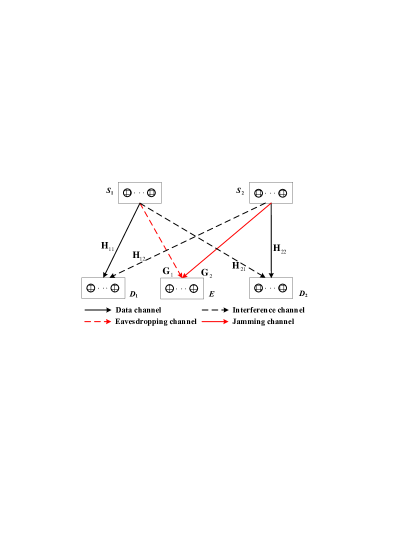
Figure 1: A MIMO two-user wiretap interference channel

III System Model and Problem Statement

We consider a MIMO interference network which consists of a wiretap channel S₁-D₁-E and a point-to-point channel S₂-D₂ (see Fig. 1). In a real setting, the former channel would correspond to a source-destination pair that needs to maintain secret communications, while the latter would correspond to a public communication system. While communicating with its intended destination, S₂ acts as a jammer to the external passive eavesdropper E. S₁ and S₂ are equipped with $N_{s}^{1}$, $N_{s}^{2}$ antennas, respectively; D₁, D₂ and E are equipped with $N_{d}^{1}$, $N_{d}^{2}$ and $N_{e}$ antennas, respectively. Let ${\bf s}_{1}\sim\mathcal{CN}(\bf{0},\bf{I})$ and ${\bf s}_{2}\sim\mathcal{CN}(\bf{0},\bf{I})$ be the messages transmitted from S₁ and S₂, respectively. Each message is precoded by a matrix before transmission. The signals received at the legitimate receiver D_i can be expressed as

$${{\bf y}_{d}^{i}}={\bf{H}}_{i1}{\bf V}{\bf s}_{1}+{{\bf{H}}_{i2}}{{\bf{W}}{\bf s}_{2}}+{{\bf{n}}_{d}^{i}},i=1,2,$$ (5)

while the signal received at the eavesdropper E can be expressed as

$${{\bf{y}}_{e}}={{\bf{G}}_{1}}{\bf V}{\bf s}_{1}+{{\bf{G}}_{2}}{{\bf{W}}{\bf s}_{2}}+{{\bf{n}}_{e}}\textrm{.}$$ (6)

Here, ${\bf{V}}\in\mathbb{C}^{N_{s}^{1}\times K_{v}}$ and ${\bf{W}}\in\mathbb{C}^{N_{s}^{2}\times K_{w}}$ are the precoding matrices at S₁ and S₂, respectively; ${{\bf{n}}_{d}^{i}}\sim\mathcal{CN}(\bf{0},\bf{I})$ and ${{\bf{n}}_{e}}\sim\mathcal{CN}(\bf{0},\bf{I})$ represent noise at the $i$th destination D_i and the eavesdropper E, respectively; ${\bf{H}}_{ij}\in\mathbb{C}^{N_{d}^{i}\times N_{s}^{j}}$, $i,j\in\{1,2\}$, denotes the channel matrix from S_j to D_i; ${\bf{G}}_{j}\in\mathbb{C}^{N_{e}\times N_{s}^{j}}$, $j\in\{1,2\}$, represents the channel matrix from S_j to E.

In this paper, we make the following assumptions:

1. The messages ${\bf s}_{1}$ and ${\bf s}_{2}$ are independent of each other, and independent of the noise vectors ${\bf n}_{d}^{i}$ and ${\bf n}_{e}$.

2. CCI is treated as noise at each receiver. We assume Gaussian signaling for S₂. Thus the MIMO wiretap channel S₁-D₁-E is Gaussian. For this case, a Gaussian input signal at S₁ is the optimal choice [33, 34].

3. All channel matrices are full rank. Global channel state information (CSI) is available, including the CSI for the eavesdropper. This is possible in situations in which the eavesdropper is an active member of the network, and thus its whereabouts and behavior can be monitored.

The achievable secrecy rate for transmitting the message ${\bf s}_{1}$ and ${\bf s}_{2}$ are respectively given as [35]

$$R_{s}^{1} =(R_{d}^{1}-R_{e})^{+},$$ (7)

$$R_{s}^{2} =R_{d}^{2}\textrm{.}$$ (8)

where

$$R_{d}^{1}={\rm{log}}|{\bf I}+({\bf I}+{\bf H}_{12}{\bf Q}_{w}{\bf H}_{12}^{H})^{-1}{\bf H}_{11}{\bf Q}_{v}{\bf H}_{11}^{H}|,$$ (9a)

$$R_{d}^{2}={\rm{log}}|{\bf I}+({\bf I}+{\bf H}_{21}{\bf Q}_{v}{\bf H}_{21}^{H})^{-1}{\bf H}_{22}{\bf Q}_{w}{\bf H}_{22}^{H}|,$$ (9b)

$$R_{e}={\rm{log}}|{\bf I}+({\bf I}+{\bf G}_{2}{\bf Q}_{w}{\bf G}_{2}^{H})^{-1}{\bf G}_{1}{\bf Q}_{v}{\bf G}_{1}^{H}|,$$ (9c)

with ${\bf Q}_{v}\triangleq{\bf{VV}}^{H}$ and ${\bf Q}_{w}\triangleq{\bf{WW}}^{H}$ denoting the transmit covariance matrices of S₁ and S₂, respectively.

The achievable secrecy rate region is the set of all secrecy rate pairs, i.e., $\mathcal{R}\buildrel\Delta\over{=}\mathop{\cup}\limits_{({\bf V},{\bf W})\in{\mathcal{I}}}(R_{s}^{1},R_{s}^{2})$, where ${\mathcal{I}}\triangleq\{({\bf V},{\bf W})|{\rm{tr}}\{{\bf{VV}}^{H}\}=P,{\rm{tr}}\{{\bf{WW}}^{H}\}=P\}$, with $P$ denoting the transmit power budget. Generally, the determination of the outer boundary of $\mathcal{R}$ is a non-convex problem. Next, we study a simpler problem, namely the achievable secrecy degrees of freedom region, defined as

$$\mathcal{D}\buildrel\Delta\over{=}\mathop{\cup}\limits_{({\bf V},{\bf W})\in{\mathcal{I}}}(d_{s}^{1},d_{s}^{2}),$$ (10)

where $d_{s}^{i}$ denotes the high SNR behavior of the achievable secrecy rate, i.e.,

$$d_{s}^{i}\triangleq\mathop{\lim}\limits_{P\to\infty}\dfrac{R_{s}^{i}}{{\rm log}\ P},i\in\{1,2\}.$$ (11)

As shown in Fig. 2, the outer boundary of $\mathcal{D}$ consists of the strict S.D.o.F. region boundary (the part between E1 and E2 in the graph) and the non-strict S.D.o.F. region boundary (the vertical part below E1 and the horizontal part up to E2 of the graph). The points marked by SU1 and SU2 correspond to single user S.D.o.F., i.e., when only one user communicates. For an arbitrary point on the strict S.D.o.F. region boundary, it is impossible to improve one S.D.o.F., without decreasing the other. On the other hand, for a point on the non-strict S.D.o.F. region boundary, one S.D.o.F. can be further improved while the other S.D.o.F. remains at the maximum value.

In the following, we will determine the outer boundary of $\mathcal{D}$, and find its connection to the number of antennas. Towards that goal, we first introduce a cooperative transmission scheme. Then, by studying that scheme we determine in closed form the outer boundary of $\mathcal{D}$ and also we construct the precoding matrices which achieve the outer boundary of $\mathcal{D}$.

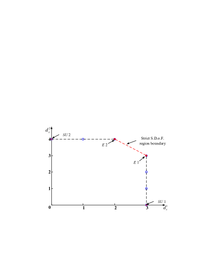
Figure 2: Achievable S.D.o.F. region boundary

IV Cooperative Secrecy Transmission Scheme

Proposition 2

For the precoding matrix pair $({\bf V},{\bf W})$, the achieved S.D.o.F. equals

$$d_{s}^{1}({\bf V},{\bf W})={\rm{rank}}\{{\bf{H}}_{11}{\bf V}\}-m({\bf V},{\bf W})-n({\bf V},{\bf W}),$$ (12a)

$$d_{s}^{2}({\bf V},{\bf W})={\rm{dim}}\{{\rm{span}}({\bf{H}}_{22}{\bf{W}})/{\rm{span}}({\bf{H}}_{21}{\bf{V}})\},$$ (12b)

in which $m({\bf V},{\bf W})\triangleq{\rm{dim}}\{{\rm{span}}({\bf{G}}_{1}{\bf{V}})/{\rm{span}}({\bf{G}}_{2}{\bf{W}})\}$ and $n({\bf V},{\bf W})\triangleq{\rm{dim}}\{{\rm{span(}}{{\bf{H}}_{12}}{\bf{W}}{\rm{)}}\cap{\rm{span}}({{\bf{H}}_{11}}{\bf{V}})\}$.

Proof:

See Appendix B. ∎

According to Proposition 2, the achievable S.D.o.F. of S₁-D₁ depends only on the dimension difference of the interference-free subspaces which D₁ and E can see. Motivated by this observation, we propose a transmission scheme in which the subspace spanned by the message signal has no intersection with the subspace spanned by the interference signal at D₁, and belongs to the subspace spanned by the interference signal at E. In this way, D₁ can see an interference-free message signal, such that $R_{d}^{1}$ scales with ${\rm{log}}(P)$, while E can only see a distorted version of the message signal, such that $R_{e}$ converges to a constant as $P$ approaches to infinity. In other words, the precoding matrix pairs belongs to the set $\bar{\mathcal{I}}$, which is defined as follows:

$$\bar{\mathcal{I}}\triangleq\{({\bf V},{\bf W})|({\bf V},{\bf W})\in\bar{\mathcal{I}}_{1}\cap\bar{\mathcal{I}}_{2}\cap{\mathcal{I}}\},$$

where

$$\bar{\mathcal{I}}_{1}\triangleq\{({\bf V},{\bf W})|{\rm{span}}({\bf{G}}_{1}{\bf{V}})\subset{\rm{span}}({\bf{G}}_{2}{\bf{W}})\},$$ (13a)

$$\bar{\mathcal{I}}_{2}\triangleq\{({\bf V},{\bf W})|{\rm{span}}({\bf{H}}_{11}{\bf{V}})\cap{\rm{span}}({\bf{H}}_{12}{\bf{W}})={\bf 0}\}.$$ (13b)

Next, we show that the proposed scheme can achieve all the boundary points of the S.D.o.F. region.

Proposition 3

Let

$$\bar{\mathcal{D}}\buildrel\Delta\over{=}\mathop{\cup}\limits_{({\bf V},{\bf W})\in\bar{\mathcal{I}}}(d_{s}^{1},d_{s}^{2})\textrm{.}$$ (14)

Then, the outer boundary of $\bar{\mathcal{D}}$ is the same as that of ${\mathcal{D}}$.

Proof:

See Appendix C. ∎

By restricting $({\bf V},{\bf W})$ to lie in $\bar{\cal I}$, we exclude a large number of precoding matrix pairs in $\cal I$, which have no contribution to the outer boundary, and thus reduce the number of precoding matrices we need to investigate in determining the outer boundary of the S.D.o.F. region. It turns out that we can reduce the set even further without changing the achievable S.D.o.F. region; this is discussed in the following corollary, where we introduce a new set $\hat{\cal I}$, which is a subset of $\bar{\cal I}$.

Corollary 1

Let

$$\hat{\mathcal{D}}\buildrel\Delta\over{=}\mathop{\cup}\limits_{({\bf V},{\bf W})\in\hat{\mathcal{I}}}(d_{s}^{1},d_{s}^{2})\textrm{,}$$ (15)

where the set of $\hat{\mathcal{I}}$ is defined as follows,

$$\hat{\mathcal{I}}\triangleq\{({\bf V},{\bf W})|{\bf{G}}_{1}{\bf{V}}={\bf{G}}_{2}{\bf{W}}(:,1:K_{v}),({\bf V},{\bf W})\in\bar{\mathcal{I}}\}.$$ (16)

Then, $\hat{\mathcal{D}}=\bar{\mathcal{D}}$.

Proof:

See Appendix D. ∎

Corollary 2

For any given precoding matrix pair $({\bf V},{\bf W})\in\bar{\mathcal{I}}$, the achieved S.D.o.F. over the wiretap channel S₁-D₁-E is $d_{s}^{1}={\rm rank}({\bf H}_{11}{\bf V})$.

Proof:

Since $({\bf V},{\bf W})\in\bar{\mathcal{I}}$, it holds that ${\rm{span}}({\bf{G}}_{1}{\bf{V}})\subset{\rm{span}}({\bf{G}}_{2}{\bf{W}})$, which indicates $\mathop{\lim}\limits_{P\to\infty}\dfrac{R_{e}}{{\rm{log}}(P)}=0$. In addition, ${\rm{span}}({\bf{H}}_{11}{\bf{V}})\cap{\rm{span}}({\bf{H}}_{12}{\bf{W}})={\bf 0}$, thus $\mathop{\lim}\limits_{P\to\infty}\dfrac{R_{d}^{1}}{{\rm{log}}(P)}={\rm rank}({\bf H}_{11}{\bf V})$. So,

$$d_{s}^{1}=\mathop{\lim}\limits_{P\to\infty}\dfrac{R_{d}^{1}}{{\rm{log}}(P)}-\mathop{\lim}\limits_{P\to\infty}\dfrac{R_{e}}{{\rm{log}}(P)}={\rm rank}({\bf H}_{11}{\bf V}).$$

This completes the proof. ∎

V Computation of the S.D.o.F. Boundary

The key idea for computing the S.D.o.F. boundary is to maximize the value of $d_{s}^{2}$ for a fixed value of $d_{s}^{1}$, say $d_{s}^{1}=\hat{d}_{s}^{1}$. Based on Corollary 1, in order to determine the outer boundary of ${\mathcal{D}}$, we only need to focus on the set $\hat{\mathcal{I}}$ (see eq. (16)). Further, Corollary 2 shows that for $({\bf V},{\bf W})\in\hat{\mathcal{I}}$ the achieved S.D.o.F. is $d_{s}^{1}={\rm{rank}}\{{\bf H}_{11}{\bf V}\}$. The problem of interest now is to construct precoding matrices which satisfy $({\bf V},{\bf W})\in\hat{\mathcal{I}}$, $K_{v}=\hat{d}_{s}^{1}$, and also leave a maximum dimension interference-free subspace for D₂.

For ease of exposition, let $({\bf v},{\bf w})$ denote the precoding vector pair. Some observations are in order. First, one can see that when the source message sent by S₁ lies in the null space of the eavesdropping channel, even if the pair S₂-D₂ communicates, their interference cannot degrade any further the eavesdropping channel because the eavesdropper already receives nothing; in those cases we may take ${\bf w}={\bf 0}$. Second, according to Corollary 2, for any precoding matrix pairs $({\bf V},{\bf W})\in\hat{\mathcal{I}}$, the achieved S.D.o.F. $d_{s}^{1}={\rm{rank}}\{{\bf H}_{11}{\bf V}\}$. Thus, a greater value of $d_{s}^{1}$ can be achieved by including more linear independent precoding vector pairs in $({\bf V},{\bf W})$. Third, the maximum number of linear precoding vector pairs is determined by (13b), which requires that

$${\rm{dim}}\{{\rm{span}}({\bf{H}}_{11}{\bf{V}})\}+{\rm{dim}}\{{\rm{span}}({\bf{H}}_{12}{\bf{W}})\}\leq N_{d}^{1}.$$ (17)

Fourth, the maximum dimension of the interference-free subspace at D₂ depends on whether D₂ experiences interference from S₁. So, in the following subsections, we will divide the set satisfying ${\bf{G}}_{1}{\bf v}={\bf{G}}_{2}{\bf w}$ into six subsets, according to whether the source message from S₁ lies in the null space of the eavesdropping channel, whether the source message from S₂ has interference on D₁, and whether the source message from S₁ has interference on D₂. Accordingly, we characterize the precoding vector pairs in each subset with the signal dimension triplet $(a,b,c)$, where $a$ and $b$ denote the number of signal dimensions we respectively need at D₁ and S₂, and $c$ denotes the signal dimension penalty at D₂, for obtaining one S.D.o.F. over the wiretap channel S₁-D₁-E. In particular, $a\triangleq{\rm{rank}}\{{\bf{H}}_{11}{\bf{v}}\}+{\rm{rank}}\{{\bf{H}}_{12}{\bf{w}}\}$; $b\triangleq{\rm{rank}}\{\bf w\}$; $c\triangleq{\rm{rank}}\{{\bf{H}}_{21}{\bf{v}}\}$. Then,

1. if the message signal sent by S₁ spreads within the null space of the eavesdropping channel, the message signal sent from S₁ is secure even without the help of S₂, thus $b=0$, $a=1$; otherwise, $b=1$.

2. if the message signal sent by S₂ interferes with D₁, we need at least two signal dimensions at D₁ in order to tell the message signal sent by S₁ apart from that sent by S₂, which means that $a=2$; otherwise, $a=1$.

3. if the message signal sent by S₁ interferes with D₂, the signal dimension penalty at D₂ is one, thus $c=1$; otherwise, $c=0$.

Please refer to Table I for the triplet $(a,b,c)$ of the precoding vector pair from each subset. Based on this triplet $(a,b,c)$, in this section, we will analyze the Single-User points SU1 and SU2, the strict S.D.o.F. region boundary, and the ending points of strict S.D.o.F. region boundary E1 and E2.

V-A Aligned signal subspace decomposition

In this subsection, we divide the set satisfying ${\bf{G}}_{1}{\bf v}={\bf{G}}_{2}{\bf w}$ into six subsets, i.e., $Sub_{\rm I}$,…, $Sub_{\rm VI}$, and determine the number of linear independent precoding vector pairs that should be considered in each subset, i.e., $d_{\rm I}$,…,$d_{\rm VI}$, respectively.

TABLE I: The triplet $(a,b,c)$ corresponding to the precoding vector pair from each subset and the number of linear independent precoding vector pairs that should be considered in each subset

subsets	(a,b,c)	maximum number of linear independent precoding vector pairs $({\bf v},{\bf w})$
$Sub_{\rm I}$	$(1,0,0)$	$d_{\rm I}=(N_{s}^{1}-N_{e}-N_{d}^{2})^{+}$
$Sub_{\rm II}$	$(1,0,1)$	$d_{\rm II}=\min\{N_{d}^{2},(N_{s}^{1}-N_{e})^{+}\}$
$Sub_{\rm III}$	$(1,1,0)$	$d_{\rm III}=(\min\{(N_{s}^{1}-N_{d}^{2})^{+},N_{e}\}+\min\{(N_{s}^{2}-N_{d}^{1})^{+},N_{e}\}-N_{e})^{+}$
$Sub_{\rm IV}$	$(1,1,1)$	$d_{\rm IV}=(\min\{N_{s}^{1},N_{e}\}+\min\{(N_{s}^{2}-N_{d}^{1})^{+},N_{e}\}-N_{e})^{+}-d_{\rm III}$
$Sub_{\rm V}$	$(2,1,0)$	$d_{\rm V}=(\min\{(N_{s}^{1}-N_{d}^{2})^{+},N_{e}\}+\min\{N_{s}^{2},N_{e}\}-N_{e})^{+}-d_{\rm III}$
$Sub_{\rm VI}$	$(2,1,1)$	$d_{\rm VI}=(\min\{N_{s}^{1},N_{e}\}+\min\{N_{s}^{2},N_{e}\}-N_{e})^{+}-(d_{\rm III}+d_{\rm IV}+d_{\rm V})$

I) The message signal sent by S₁ spreads within the null space of the eavesdropping channel, and does not interfere with D₂. That is, the precoding vector pairs in $Sub_{\rm I}$ should satisfy

$${\bf{G}}_{1}{\bf v}={\bf 0},$$ (18a)

$${\bf{H}}_{21}{\bf v}={\bf 0}.$$ (18b)

Further, it holds that ${\bf{G}}_{2}{\bf w}={\bf{G}}_{1}{\bf v}={\bf 0}$. The case where ${\bf{G}}_{1}{\bf v}={\bf{G}}_{2}{\bf w}=0$ and ${\bf w}\neq 0$ is not considered here, because even if the pair S₂-D₂ communicates, their interference cannot degrade any further the eavesdropping channel. So we will consider ${\bf w}={\bf 0}$ for simplicity. Substituting ${\bf v}={\bf\Gamma}({\bf G}_{1}){\bf x}$ into (18b), with $\bf x$ being any vectors with appropriate length, we arrive at ${\bf{H}}_{21}{\bf\Gamma}({\bf G}_{1}){\bf x}={\bf 0}$, which is equivalent to ${\bf x}={\bf\Gamma}({\bf{H}}_{21}{\bf\Gamma}({\bf G}_{1})){\bf y}$, with $\bf y$ being any vectors with appropriate length. Therefore, the formula of $\bf v$ in $Sub_{\rm I}$ is

$${\bf v}={\bf\Gamma}({\bf G}_{1}){\bf\Gamma}({\bf{H}}_{21}{\bf\Gamma}({\bf G}_{1})){\bf z},$$ (19)

with $\bf z$ being any nonzero vectors with appropriate length. In addition, since all the channel matrices are assumed to be full rank, it holds that

$$d_{\rm I}\leq{\rm{dim}}\{{\rm{null}}({{\bf H}_{21}{\bf\Gamma}}({\bf{G}}_{1}))\}=(N_{s}^{1}-N_{e}-N_{d}^{2})^{+}.$$ (20)

II) The message signal sent by S₁ spreads within the null space of the eavesdropping channel, but does interfere with D₂. That is, the vectors in $Sub_{\rm II}$ should satisfy

$${\bf{G}}_{1}{\bf v}={\bf 0},$$ (21a)

$${\bf{H}}_{21}{\bf v}\neq{\bf 0}.$$ (21b)

Here again, we will consider ${\bf w}={\bf 0}$ for simplicity. On combining (18a)-(18b) with (21a)-(21b), it holds that

$$Sub_{\rm I}\cup Sub_{\rm II}=\{({\bf v},{\bf w})|{\bf{G}}_{1}{\bf v}={\bf 0},{\bf w}={\bf 0}\}.$$ (22)

So, the linear independent vectors we can choose from $Sub_{\rm I}$ and $Sub_{\rm II}$ should be no greater than ${\rm{dim}}\{{\rm{null}}({\bf{G}}_{1})\}$. That is,

$$d_{\rm II}+d_{\rm I}\leq(N_{s}^{1}-N_{e})^{+}.$$ (23)

III) The message signal sent by S₁ does not spread within the null space of the eavesdropping channel. The message signals sent by S₁ and S₂ do not interfere with D₂ and D₁, respectively. That is, the precoding vector pairs in $Sub_{\rm III}$ should satisfy

$${\bf{H}}_{12}{\bf w}={\bf 0},$$ (24a)

$${\bf{H}}_{21}{\bf v}={\bf 0},$$ (24b)

$${\bf{G}}_{1}{\bf v}={\bf{G}}_{2}{\bf w}\neq{\bf 0}.$$ (24c)

Substituting ${\bf v}={\bf\Gamma}({\bf H}_{21}){\bf x}$ and ${\bf w}={\bf\Gamma}({\bf H}_{12}){\bf y}$ into (24c), we arrive at

$${\bf{G}}_{1}{\bf\Gamma}({\bf H}_{21}){\bf x}={\bf{G}}_{2}{\bf\Gamma}({\bf H}_{12}){\bf y}\neq{\bf 0}.$$ (25)

Consider the decomposition

$${\rm{GSVD}}({\bf{G}}_{1}{\bf\Gamma}({\bf H}_{21}),{\bf{G}}_{2}{\bf\Gamma}({\bf H}_{12});N_{e},\hat{N}_{s}^{1},\hat{N}_{s}^{2})$$

$$\quad\quad=(\hat{\bf\Psi}_{1},\hat{\bf\Psi}_{2},\hat{\bf\Lambda}_{1},\hat{\bf\Lambda}_{2},\hat{\bf X},\hat{k},\hat{r},\hat{s},\hat{p}),$$

where $\hat{N}_{s}^{1}\triangleq(N_{s}^{1}-N_{d}^{2})^{+}$ and $\hat{N}_{s}^{2}\triangleq(N_{s}^{2}-N_{d}^{1})^{+}$. Applying Proposition 1, we can obtain the number of linearly independent vectors $\bf v$ satisfying (25), i.e.,

$$\hat{d}_{\rm III}\triangleq\hat{s}+{\rm{dim}}\{{\rm{null}}({\bf{G}}_{1}{\bf\Gamma}({\bf H}_{21}))\}.$$

Since ${\rm{null}}({\bf{G}}_{1}{\bf\Gamma}({\bf H}_{21}))={\rm{null}}({{\bf H}_{21}{\bf\Gamma}}({\bf{G}}_{1}))$, the basis of ${\rm{null}}({\bf{G}}_{1}{\bf\Gamma}({\bf H}_{21}))$ also spans the solution space of $\bf v$ in $Sub_{\rm I}$. Thus,

$$d_{\rm III}+d_{\rm I}\leq\hat{d}_{\rm III}=\hat{s}+(N_{s}^{1}-N_{e}-N_{d}^{2})^{+},$$ (26)

IV) The message signal sent by S₁ does not spread within the null space of the eavesdropping channel. The message signal sent by S₂ does not interfere with D₁, but the message signal sent by S₁ interferes with D₂. That is, the precoding vector pairs in $Sub_{\rm IV}$ should satisfy

$${\bf{H}}_{12}{\bf w}={\bf 0},$$ (27a)

$${\bf{H}}_{21}{\bf v}\neq{\bf 0},$$ (27b)

$${\bf{G}}_{1}{\bf v}={\bf{G}}_{2}{\bf w}\neq{\bf 0}.$$ (27c)

Substituting ${\bf w}={\bf\Gamma}({\bf{H}}_{12}){\bf y}$ into (27c), we get

$${\bf{G}}_{1}{\bf v}={\bf{G}}_{2}{\bf\Gamma}({\bf{H}}_{12}){\bf y}\neq{\bf 0}.$$ (28)

Consider the decomposition

$${\rm{GSVD}}({\bf{G}}_{1},{\bf{G}}_{2}{\bf\Gamma}({\bf H}_{12});N_{e},N_{s}^{1},\hat{N}_{s}^{2})$$

$$\quad\quad=(\bar{\bf\Psi}_{1},\bar{\bf\Psi}_{2},\bar{\bf\Lambda}_{1},\bar{\bf\Lambda}_{2},\bar{\bf X},\bar{k},\bar{r},\bar{s},\bar{p}).$$

Applying Proposition 1 we can obtain the number of linearly independent vectors $\bf v$ satisfying (28), i.e.,

$$\hat{d}_{\rm IV}\triangleq\bar{s}+{\rm{dim}}\{{\rm{null}}({\bf{G}}_{1})\}.$$

On combining (24a)-(24c) with (27a)-(27c), it holds that

$$Sub_{\rm III}\cup Sub_{\rm IV}=\{({\bf v},{\bf w})|{\bf{H}}_{12}{\bf w}={\bf 0},{\bf{G}}_{1}{\bf v}={\bf{G}}_{2}{\bf w}\neq{\bf 0}\}$$

In addition, the basis of ${\rm{null}}({\bf{G}}_{1})$ also spans the solution space of $\bf v$ in $Sub_{\rm I}\cup Sub_{\rm II}$. Therefore,

$$d_{\rm IV}+d_{\rm III}+d_{\rm II}+d_{\rm I}\leq\hat{d}_{\rm IV}=\bar{s}+(N_{s}^{1}-N_{e})^{+}.$$ (29)

V) The message signal sent by S₁ does not spread within the null space of the eavesdropping channel. The message signal sent by S₂ interferes with D₁, but the message signal sent by S₁ does not interfere with D₂. That is, the precoding vector pairs in $Sub_{\rm V}$ should satisfy

$${\bf{H}}_{12}{\bf w}\neq{\bf 0},$$ (30a)

$${\bf{H}}_{21}{\bf v}={\bf 0},$$ (30b)

$${\bf{G}}_{1}{\bf v}={\bf{G}}_{2}{\bf w}\neq{\bf 0}.$$ (30c)

Substituting ${\bf v}={\bf\Gamma}({\bf{H}}_{21}){\bf x}$ into (30c), we obtain

$${\bf{G}}_{1}{\bf\Gamma}({\bf{H}}_{21}){\bf x}={\bf{G}}_{2}{\bf w}\neq{\bf 0}.$$ (31)

Consider the decomposition

$${\rm{GSVD}}({\bf{G}}_{1}{\bf\Gamma}({\bf H}_{21}),{\bf{G}}_{2};N_{e},\hat{N}_{s}^{1},N_{s}^{2})$$

$$\quad\quad=(\breve{\bf\Psi}_{1},\breve{\bf\Psi}_{2},\breve{\bf\Lambda}_{1},\breve{\bf\Lambda}_{2},\breve{\bf X},\breve{k},\breve{r},\breve{s},\breve{p}).$$

Applying Proposition 1, we can obtain the number of linearly independent vectors $\bf v$ satisfying (31), i.e.,

$$\hat{d}_{\rm V}\triangleq\breve{s}+{\rm{dim}}\{{\rm{null}}({\bf{G}}_{1}{\bf\Gamma}({\bf H}_{21}))\}.$$

On combining (24a)-(24c) with (30a)-(30c), it holds that

$$Sub_{\rm III}\cup Sub_{\rm V}=\{({\bf v},{\bf w})|{\bf{H}}_{21}{\bf v}={\bf 0},{\bf{G}}_{1}{\bf v}={\bf{G}}_{2}{\bf w}\neq{\bf 0}\}$$

In addition, the basis of ${\rm{null}}({\bf{G}}_{1}{\bf\Gamma}({\bf H}_{21}))$ also spans the solution space of $\bf v$ in $Sub_{\rm I}$. Therefore,

$$d_{\rm V}+d_{\rm III}+d_{\rm I}\leq\hat{d}_{\rm V}=\breve{s}+(N_{s}^{1}-N_{e}-N_{d}^{2})^{+}.$$ (32)

VI) The message signal sent by S₁ does not spread within the null space of the eavesdropping channel. The message signals sent by S₂ and S₁ interfere with D₁ and D₂, respectively. That is, the precoding vector pairs in $Sub_{\rm VI}$ should satisfy

$${\bf{H}}_{12}{\bf w}\neq{\bf 0},$$ (33a)

$${\bf{H}}_{21}{\bf v}\neq{\bf 0},$$ (33b)

$${\bf{G}}_{1}{\bf v}={\bf{G}}_{2}{\bf w}\neq{\bf 0}.$$ (33c)

Consider the decomposition

$${\rm{GSVD}}({\bf{G}}_{1},{\bf{G}}_{2};N_{e},N_{s}^{1},N_{s}^{2})=(\tilde{\bf\Psi}_{1},\tilde{\bf\Psi}_{2},\tilde{\bf\Lambda}_{1},\tilde{\bf\Lambda}_{2},\tilde{\bf X},\tilde{k},\tilde{r},\tilde{s},\tilde{p}).$$

According to Proposition 1, we can obtain the number of linearly independent vectors $\bf v$ satisfying (33c), i.e.,

$$d_{s}\triangleq\tilde{s}+{\rm{dim}}\{{\rm{null}}({\bf{G}}_{1})\}.$$

On combining (33a)-(33c) with (24a)-(24c), (27a)-(27c) and (30a)-(30c), it holds that $Sub_{\rm III}\cup Sub_{\rm IV}\cup Sub_{\rm V}\cup Sub_{\rm VI}=\{({\bf v},{\bf w})|{\bf{G}}_{1}{\bf v}={\bf{G}}_{2}{\bf w}\neq{\bf 0}\}$. In addition, the basis of ${\rm{null}}({\bf{G}}_{1})$ also spans the solution space of $\bf v$ in $Sub_{\rm I}\cup Sub_{\rm II}$. Thus,

$$d_{\rm VI}+d_{\rm V}+d_{\rm IV}+d_{\rm III}+d_{\rm II}+d_{\rm I}\leq d_{s}.$$ (34)

We should note that with all three variables smaller than the corresponding variables of other triplets, the precoding vector pair from $Sub_{\rm I}$ has the potential to achieve a greater S.D.o.F. than the others, and so it has the highest priority in the construction of $({\bf V},{\bf W})$. Similarly, the precoding vector pair from $Sub_{\rm IV}$ has lower priority than that one from $Sub_{\rm I}\cup Sub_{\rm II}\cup Sub_{\rm III}$; the precoding vector pair from $Sub_{\rm V}$ has lower priority than that one from $Sub_{\rm I}\cup Sub_{\rm III}$; and the precoding vector pair from $Sub_{\rm VI}$ has the lowest priority. Therefore, all the equalities in (20), (23), (26), (29), (32) and (34) hold true. As a conclusion, the number of linear independent precoding vector pairs that should be considered in each subset is given in Table I.

Correspondingly, in what follows, we give the formulas of $\bf v$ and $\bf w$ we consider in each subset. Combining the formula of $\bf v$ in $Sub_{\rm I}$, i.e., (19), and that one in $Sub_{\rm I}\cup Sub_{\rm II}$, i.e., (22), we obtain the one in $Sub_{\rm II}$, i.e.,

$${\bf v}={\bf\Gamma}({\bf G}_{1}){\bf\Gamma}^{\perp}({\bf{H}}_{21}{\bf\Gamma}({\bf G}_{1})){\bf z}+{\bf\Gamma}({\bf G}_{1}){\bf\Gamma}({\bf{H}}_{21}{\bf\Gamma}({\bf G}_{1})){\bf y}.$$

with $\bf z$ being any nonzero vectors with appropriate length. Since we want linear independent precoding vectors, the beamforming direction already considered in the set with higher priority, e.g., $Sub_{\rm I}$, should not be under consideration in other subsets. Thus, the formula of $\bf v$ in $Sub_{\rm II}$ is

$${\bf v}={\bf\Gamma}({\bf G}_{1}){\bf\Gamma}^{\perp}({\bf{H}}_{21}{\bf\Gamma}({\bf G}_{1})){\bf z}.$$ (35)

Similarly, the formulas of $\bf v$ and $\bf w$ in $Sub_{\rm III}$ are, respectively,

$${\bf v}=\hat{\bf\Psi}_{12}\hat{\bf\Lambda}_{1}^{-1}{\bf z},{\bf w}=\hat{\bf\Psi}_{22}\hat{\bf\Lambda}_{2}^{-1}{\bf z}.$$ (36)

The formulas of $\bf v$ and $\bf w$ in $Sub_{\rm IV}$ are, respectively,

$${\bf v}=\bar{\bf\Psi}_{12}\bar{\bf\Lambda}_{1}^{-1}{\bf z},{\bf w}=\bar{\bf\Psi}_{22}\bar{\bf\Lambda}_{2}^{-1}{\bf z}.$$ (37)

The formulas of $\bf v$ and $\bf w$ in $Sub_{\rm V}$ are, respectively,

$${\bf v}=\breve{\bf\Psi}_{12}\breve{\bf\Lambda}_{1}^{-1}{\bf z},{\bf w}=\breve{\bf\Psi}_{22}\breve{\bf\Lambda}_{2}^{-1}{\bf z}.$$ (38)

And the formulas of $\bf v$ and $\bf w$ in $Sub_{\rm VI}$ are, respectively,

$${\bf v}=\tilde{\bf\Psi}_{12}\tilde{\bf\Lambda}_{1}^{-1}{\bf z},{\bf w}=\tilde{\bf\Psi}_{22}\tilde{\bf\Lambda}_{2}^{-1}{\bf z}.$$ (39)

We should note that since ${\bf H}_{21}$ is independent of the channels ${\bf{G}}_{1}$, ${\bf{G}}_{2}$ and ${\bf H}_{12}$, for precoding vector pairs in (37) ${\bf H}_{21}{\bf v}\neq 0$ holds true with probability one. Similar argument also applies in the derivation of the formulas of $\bf v$ and $\bf w$ in $Sub_{\rm V}$ and $Sub_{\rm VI}$.

V-B Single-User points SU1($\bar{d}_{s}^{1}$, 0) and SU2(0, $\bar{d}_{s}^{2}$)

A single-user point corresponds to a scenario in which only one source-destination communicates. Let $\bar{d}_{s}^{1}$ and $\bar{d}_{s}^{2}$ denote the maximum achievable value of $d_{s}^{1}$ and $d_{s}^{2}$, respectively.

V-B1 The single-user point SU1($\bar{d}_{s}^{1}$, 0)

In this case, the pair S₂-D₂ does not communicate, but S₂ still transmits, acting as a cooperative jammer targeting at degrading the eavesdropping channel. In this case, the system model reduces to a wiretap channel with a cooperative jammer. Based on Corollary 1 and Corollary 2, we see that our problem for maximizing $d_{s}^{1}$ is including as more precoding vector pairs as possible in $({\bf V},{\bf W})$. In Table I, we divide the set which satisfies ${\bf G}_{1}{\bf v}={\bf G}_{2}{\bf w}$ into six subsets. Due to the requirement in (17), it holds that more precoding vector pairs can be included in $({\bf V},{\bf W})$ by choosing precoding vector pairs from the subsets with smaller $a$. For example, $a=1$ for $Sub_{\rm IV}$ while $a=2$ for $Sub_{\rm VI}$. We can select at most $N_{d}^{1}$ precoding vector pairs from $Sub_{\rm IV}$, in which $a=1$, while we can select only $\lfloor N_{d}^{1}/2\rfloor$ precoding vector pairs from $Sub_{\rm VI}$, in which $a=2$. In addition, since the achieved S.D.o.F. is $d_{s}^{1}={\rm{rank}}\{{\bf H}_{11}{\bf V}\}$, a greater value of $d_{s}^{1}$ can be achieved with precoding vector pairs from $Sub_{\rm IV}$. Therefore, in the construction of $({\bf V},{\bf W})$, the precoding vector pairs from the first four subsets have the same priority, and the precoding vector pairs from the last two subsets have the same priority. Moreover, a precoding vector pair from the first four subsets has higher priority than that one from the last two subsets. If $N_{d}^{1}\leq d_{\rm I}+d_{\rm II}+d_{\rm III}+d_{\rm IV}$, we just select $N_{d}^{1}$ precoding vector pairs from $Sub_{\rm I}\cup Sub_{\rm II}\cup Sub_{\rm III}\cup Sub_{\rm IV}$; otherwise, we first select all the precoding vector pairs in $Sub_{\rm I}\cup Sub_{\rm II}\cup Sub_{\rm III}\cup Sub_{\rm IV}$, and then we pick $\lfloor\dfrac{N_{d}^{1}-(d_{\rm I}+d_{\rm II}+d_{\rm III}+d_{\rm IV})}{2}\rfloor$ precoding vector pairs from $Sub_{\rm V}\cup Sub_{\rm VI}$.

Example 1: Consider the case $(N_{s}^{1},N_{d}^{1},N_{e})=(6,3,6)$, $(N_{s}^{2},N_{d}^{2})=(6,6)$. Based on Table I, the maximum number of linear independent precoding vector pairs in each subset is $d_{\rm I}=0$, $d_{\rm II}=0$, $d_{\rm III}=0$, $d_{\rm IV}=3$, $d_{\rm V}=0$, $d_{\rm VI}=3$. Since $N_{d}^{1}=d_{\rm I}+d_{\rm II}+d_{\rm III}+d_{\rm IV}$, we first select three precoding vector pairs in $Sub_{\rm IV}$. We cannot pick any more precoding vector pairs without violating (17) since in that case the the remaining signal dimension at D₁ is $N_{d}^{1}-d_{\rm IV}=0$. Concluding, we can select a total of 3 precoding vector pairs, and based on Corollary 2, $\bar{d}_{s}^{1}=3$.

Example 2: Consider the case $(N_{s}^{1},N_{d}^{1},N_{e})=(6,5,5)$, $(N_{s}^{2},N_{d}^{2})=(6,4)$. Based on Table I we get that $d_{\rm I}=0$, $d_{\rm II}=1$, $d_{\rm III}=0$, $d_{\rm IV}=1$, $d_{\rm V}=2$, $d_{\rm VI}=2$. Since $N_{d}^{1}>d_{\rm I}+d_{\rm II}+d_{\rm III}+d_{\rm IV}$, we first select all the precoding vector pairs in $Sub_{\rm II}$ and $Sub_{\rm IV}$, i.e., $({\bf v}_{1},{\bf w}_{1})$, $({\bf v}_{2},{\bf w}_{2})$, with ${\bf H}_{12}{\bf w}_{1}=0$ and ${\bf H}_{12}{\bf w}_{2}=0$. From the remaining sets $Sub_{\rm V}$ and $Sub_{\rm VI}$, we can at most pick one pair, i.e., $({\bf v}_{3},{\bf w}_{3})$. For either $Sub_{\rm V}$ or $Sub_{\rm VI}$, it holds that ${\bf H}_{12}{\bf w}_{3}\neq 0$. Thus, for ${\bf V}=[{\bf v}_{1}\ {\bf v}_{2}\ {\bf v}_{3}]$ and ${\bf W}=[{\bf w}_{1}\ {\bf w}_{2}\ {\bf w}_{3}]$ it holds that ${\rm dim}\{{\rm span}({\bf H}_{11}{\bf V})\}+{\rm dim}\{{\rm span}({\bf H}_{12}{\bf W})\}=3+1=4$. If we picked another pair, (17) would be violated. Concluding, we can select a total of 3 precoding vector pairs, and based on Corollary 2, $\bar{d}_{s}^{1}=3$.

Summarizing, the maximum achievable value $\bar{d}_{s}^{1}$, i.e.,

$$\bar{d}_{s}^{1}=\min\{d_{a=1}+d_{a=2}^{\star},N_{d}^{1}\},$$ (40)

where $d_{a=1}=d_{\rm I}+d_{\rm II}+d_{\rm III}+d_{\rm IV}$, and

$$d_{a=2}^{\star}=\min\{d_{\rm V}+d_{\rm VI},\lfloor{(N_{d}^{1}-d_{a=1})^{+}}/{2}\rfloor\}\textrm{.}$$

Remark 1: To gain more insight into $\bar{d}_{s}^{1}$, we give Table II which shows the dependence of $\bar{d}_{s}^{1}$ on the number of antennas.

TABLE II: Summary of the closed-form results on $\bar{d}_{s}^{1}$

Inequalities on the number of antennas at terminals	$\bar{d}_{s}^{1}$
$N_{s}^{1}\geq N_{e}+N_{d}^{1}$
$N_{s}^{2}\geq N_{e}+N_{d}^{1}$	$\min\{N_{s}^{1},N_{d}^{1}\}$
$2N_{d}^{1}+N_{e}-N_{s}^{2}\leq N_{s}^{1}<N_{e}+N_{d}^{1}$
$N_{d}^{1}<N_{s}^{2}<N_{e}+N_{d}^{1}$
$N_{d}^{1}+N_{e}-N_{s}^{2}<N_{s}^{1}<2N_{d}^{1}+N_{e}-N_{s}^{2}$	$N_{s}^{1}+N_{s}^{2}-(N_{d}^{1}+N_{e})+\min\{s,\lfloor\frac{2N_{d}^{1}+N_{e}-N_{s}^{1}-N_{s}^{2}}{2}\rfloor\}$
$N_{d}^{1}<N_{s}^{2}<N_{e}+N_{d}^{1}$	$s=\min\{N_{d}^{1}+N_{e}-N_{s}^{2},N_{e}\}+\min\{N_{s}^{2},N_{e}\}-N_{e}$
$N_{e}<N_{s}^{1}<N_{e}+N_{d}^{1}$, $N_{s}^{2}\leq N_{d}^{1}$	$N_{s}^{1}-N_{e}+\min\{s,\lfloor\frac{N_{d}^{1}+N_{e}-N_{s}^{1}}{2}\rfloor\}$, $s=\min\{N_{s}^{2},N_{e}\}$
$N_{s}^{1}\leq N_{d}^{1}+N_{e}-N_{s}^{2}$, $N_{d}^{1}<N_{s}^{2}<N_{e}+N_{d}^{1}$	$\min\{s,\lfloor\frac{N_{d}^{1}}{2}\rfloor\}$
$N_{s}^{1}\leq N_{e}$, $N_{s}^{2}\leq N_{d}^{1}$	$s=\min\{N_{s}^{1},N_{e}\}+\min\{N_{s}^{2},N_{e}\}-\min\{N_{s}^{1}+N_{s}^{2},N_{e}\}$

V-B2 The single-user point of SU2(0, $\bar{d}_{s}^{2}$)

In this case, the wiretap channel S₁-D₁-E does not work. For a point-to-point MIMO user, the maximum achievable degrees of freedom equals $\min\{N_{s}^{2},N_{d}^{2}\}$. That is,

$$\bar{d}_{s}^{2}=\min\{N_{s}^{2},N_{d}^{2}\}.$$ (41)

V-C Computation of the strict S.D.o.F. region boundary

The key idea for computing the strict S.D.o.F. boundary is to maximize the value of $d_{s}^{2}$ for a fixed value of $d_{s}^{1}$.

Assume that ${\bf V}$ consists of $\hat{d}_{s}^{1}$ columns, among which $z$ columns come from a subset for which the message signal sent by S₁ interferes with D₂. Then, D₂ can at most see a $(N_{d}^{2}-z)^{+}$-dimension interference-free subspace. Thus,

$$\hat{d}_{s}^{2}(z)\leq(N_{d}^{2}-z)^{+}.$$ (42)

In addition, it holds that $\hat{d}_{s}^{1}+{\rm{dim}}\{{\rm{span}}({\bf{H}}_{12}{\bf{W}})\}\leq N_{d}^{1}$ due to (17). So,

$${\rm rank}\{{\bf W}\}\leq(\max\{N_{s}^{2},N_{d}^{1}\}-\hat{d}_{s}^{1})^{+}.$$ (43)

Combining (41), (42) and (43), we get the maximum achievable value of $d_{s}^{2}$, i.e.,

$$\hat{d}_{s}^{2}(z)=\min\{N_{s}^{2},(\max\{N_{s}^{2},N_{d}^{1}\}-\hat{d}_{s}^{1})^{+},(N_{d}^{2}-z)^{+}\}.$$ (44)

Thus, in order to maximize the value of $d_{s}^{2}$, we only need to minimize the value of $z$.

According to Table I, the minimum value of $z$ without the constraint $d_{s}^{1}=\hat{d}_{s}^{1}$ equals $(\hat{d}_{s}^{1}-(d_{\rm V}+d_{\rm I}+d_{\rm III}))^{+}$. Due to the constraint $d_{s}^{1}=\hat{d}_{s}^{1}$ and the fact that $a=2$ in $Sub_{\rm V}$, we have limitations on the number of pairs that can be selected from $Sub_{\rm V}$. For example, consider the case $d_{\rm I}+d_{\rm III}=2$, $d_{\rm V}=2$, $N_{d}^{1}=3$ and $\hat{d}_{s}^{1}=3$. The minimum value of $z$ without the constraint $d_{s}^{1}=\hat{d}_{s}^{1}=3$ equals $0$, in which case we need at least choose one pair from $Sub_{\rm V}$. Noting that (17) should be satisfied for $({\bf V},{\bf W})\in\hat{\cal I}$ and $a=2$ in $Sub_{\rm V}$, if we have picked one pair from $Sub_{\rm V}$, we can then at most pick one more pair from the first four subsets. Thus, the maximum achievable value of $d_{s}^{1}$ equals 2, which violates the constraint $d_{s}^{1}=3$. Due to the constraint $d_{s}^{1}=3$ and the fact that $a=2$ in $Sub_{\rm V}$, we cannot select any pairs from $Sub_{\rm V}$, and so the minimum value of $z$ equals to 1.

Let $x$ and $y$ denote the number of columns which come from the first four subsets and the last two subsets, respectively. The maximum allowable value of $y$ under the constraint of $d_{s}^{1}=\hat{d}_{s}^{1}$ is

$$y_{\max}\triangleq \max_{x,y}\quad y$$

$${\rm s.t.}\quad x+y=\hat{d}_{s}^{1},$$ (45a)

$$x+2y\leq N_{d}^{1},$$ (45b)

$$0\leq x\leq d_{\rm I}+d_{\rm II}+d_{\rm III}+d_{\rm IV},$$ (45c)

$$0\leq y\leq d_{\rm V}+d_{\rm VI}.$$ (45d)

Substituting $x=\hat{d}_{s}^{1}-y$ into (45b), we arrive at $y\leq N_{d}^{1}-\hat{d}_{s}^{1}$, which combined with (45c) and (45d) gives

$$y_{\max}=\min\{N_{d}^{1}-\hat{d}_{s}^{1},d_{\rm V}+d_{\rm VI},\hat{d}_{s}^{1}\}.$$ (46)

Thus, we can select at most $\min\{y_{\max},d_{\rm V}\}$ precoding vector pairs from $Sub_{\rm V}$. Therefore, the minimum value of $z$ is,

$$z_{\min}(\hat{d}_{s}^{1})=(\hat{d}_{s}^{1}-(\min\{y_{\max},d_{\rm V}\}+d_{\rm I}+d_{\rm III}))^{+}.$$ (47)

Substituting (47) into (44), we obtain the maximum value of $d_{s}^{2}$, i.e.,

$$\hat{d}_{s}^{2}=\min\{N_{s}^{2},(\max\{N_{s}^{2},N_{d}^{1}\}-\hat{d}_{s}^{1})^{+},(N_{d}^{2}-z_{\min}(\hat{d}_{s}^{1}))^{+}\}.$$ (48)

Remark 2: For any given values of $d_{s}^{1}$, we can derive a maximum achievable value of $d_{s}^{2}$ based on (48). Finally, the strict S.D.o.F. region boundary can be computed based on the following iteration:

1. Initialize $\hat{d}_{s}^{1}=\bar{d}_{s}^{1}$;

2. Compute $\hat{d}_{s}^{2}$ with (48);

3. Compare $\hat{d}_{s}^{2}$ with $\bar{d}_{s}^{2}$. If $\hat{d}_{s}^{2}<\bar{d}_{s}^{2}$, let $\hat{d}_{s}^{1}=\hat{d}_{s}^{1}-1$ and go to 2); otherwise, stop and output all the pairs $(\hat{d}_{s}^{1},\hat{d}_{s}^{2})$.

Example 3: Let us revisit Example 2, for which we obtained $\bar{d}_{s}^{1}=3$ and $\bar{d}_{s}^{2}=4$, respectively. Initialize $\hat{d}_{s}^{1}$ with $\bar{d}_{s}^{1}=3$. Substituting $\hat{d}_{s}^{1}=3$ into (48), we obtain $\hat{d}_{s}^{2}=3$. Since $\hat{d}_{s}^{2}<\bar{d}_{s}^{2}$, we continue the iteration. Letting $\hat{d}_{s}^{1}=2$ and substituting it into (48), we obtain $\hat{d}_{s}^{2}=4$, which equals $\bar{d}_{s}^{2}$. So, we stop the iteration and output all the S.D.o.F. pairs on the strict S.D.o.F. region boundary, i.e., $(\hat{d}_{s}^{1},\hat{d}_{s}^{2})=(3,3)$ and $(\hat{d}_{s}^{1},\hat{d}_{s}^{2})=(2,4)$.

V-D Ending points of strict S.D.o.F. region boundary E1($\bar{d}_{s}^{1}$, $\underline{d}_{s}^{2}$) and E2($\underline{d}_{s}^{1}$, $\bar{d}_{s}^{2}$)

As shown in Fig. 2, E1 and E2 denote the ending points of the strict S.D.o.F. region boundary. In particular, $\underline{d}_{s}^{2}$ denotes the maximum achievable value of ${d}_{s}^{2}$ under the constraint ${d}_{s}^{1}=\bar{d}_{s}^{1}$, and $\underline{d}_{s}^{1}$ denotes the maximum achievable value of ${d}_{s}^{1}$ under the constraint ${d}_{s}^{2}=\bar{d}_{s}^{2}$.

1) The ending point E1($\bar{d}_{s}^{1}$, $\underline{d}_{s}^{2}$). According to (40), we obtain $\bar{d}_{s}^{1}$ which denotes the maximum achievable value of $d_{s}^{1}$. Substituting $\hat{d}_{s}^{1}=\bar{d}_{s}^{1}$ into (46)-(48), we arrive at

$$\underline{d}_{s}^{2}=\min\{N_{s}^{2},(\max\{N_{s}^{2},N_{d}^{1}\}-\bar{d}_{s}^{1})^{+},(N_{d}^{2}-z_{\min}(\bar{d}_{s}^{1}))^{+}\}.$$ (49)

2) The ending point E2($\underline{d}_{s}^{1}$, $\bar{d}_{s}^{2}$). According to the previous analysis on the single-user point of SU2(0, $\bar{d}_{s}^{2}$), we obtain $\bar{d}_{s}^{2}=\min\{N_{s}^{2},N_{d}^{2}\}$, which, combined with (44), gives

$$\min\{N_{s}^{2},N_{d}^{2}\}\leq\max\{N_{s}^{2},N_{d}^{1}\}-\underline{d}_{s}^{1},$$ (50a)

$$\min\{N_{s}^{2},N_{d}^{2}\}\leq N_{d}^{2}-z.$$ (50b)

In the following, we consider two distinct cases.

(i) For the case of $N_{s}^{2}>N_{d}^{2}$, (50a) becomes

$$\underline{d}_{s}^{1}\leq\max\{N_{s}^{2},N_{d}^{1}\}-N_{d}^{2}.$$ (51)

Besides, (50b) indicates that $z=0$, and thus all of the signal steams sent by S₁ should not interfere with D₂. That is, $Sub_{\rm II}$, $Sub_{\rm IV}$ and $Sub_{\rm VI}$ are not under consideration. Applying (40), we obtain

$$\underline{d}_{s}^{1}\leq\min\{d_{\rm I}+d_{\rm III}+\beta^{\star},N_{d}^{1}\},$$ (52)

where$\beta^{\star}=\min\{d_{\rm V},\lfloor{(N_{d}^{1}-d_{\rm I}-d_{\rm III})^{+}}/{2}\rfloor\}$. Combining (51) and (52), we arrive at

$$\underline{d}_{s}^{1}=\min\{d_{\rm I}+d_{\rm III}+\beta^{\star},\max\{N_{s}^{2},N_{d}^{1}\}-N_{d}^{2},N_{d}^{1}\}.$$ (53)

(ii) For the case of $N_{s}^{2}\leq N_{d}^{2}$, (50a) becomes

$$\underline{d}_{s}^{1}\leq\max\{N_{s}^{2},N_{d}^{1}\}-N_{s}^{2},$$ (54)

which indicates that $\underline{d}_{s}^{1}=0$ when $N_{s}^{2}\geq N_{d}^{1}$. So, in the following, we only consider the case of $N_{s}^{2}<N_{d}^{1}$, where it holds that $d_{\rm III}=d_{\rm IV}=0$. In addition, (50b) indicates that $z\leq N_{d}^{2}-N_{s}^{2}.$ Therefore, $\xi=\min\{d_{\rm VI},(N_{d}^{2}-N_{s}^{2}-d_{\rm II})^{+}\}+d_{\rm V}$, where $\xi$ denotes the maximum number of precoding vector pairs that can be chosen from $Sub_{\rm V}$ and $Sub_{\rm VI}$. Applying (40), we get

$$\underline{d}_{s}^{1}\leq\min\{d_{\rm I}+\hat{d}_{\rm II}+\xi^{\star},N_{d}^{1}\},$$ (55)

where $\hat{d}_{\rm II}=\min\{N_{d}^{2}-N_{s}^{2},d_{\rm II}\}$, and

$$\xi^{\star}=\min\{\xi,\lfloor{(N_{d}^{1}-d_{\rm I}-\hat{d}_{\rm II})^{+}}/{2}\rfloor\}\textrm{.}$$

Combining (54) and (55), we arrive at

$$\underline{d}_{s}^{1}=\min\{d_{\rm I}+\hat{d}_{\rm II}+\xi^{\star},\max\{N_{s}^{2},N_{d}^{1}\}-N_{s}^{2}\}.$$ (57)

We should note that this expression also applies to the case of $N_{s}^{2}\geq N_{d}^{1}$, where $\underline{d}_{s}^{1}=0$.

Summarizing the above two cases, we arrive at

$$\underline{d}_{s}^{1}=\left\{{\begin{array}[]{*{20}{c}}{\min\{d_{\rm I}+d_{\rm III}+\beta^{\star},\eta-N_{d}^{2},N_{d}^{1}\}},{\rm{if}}\ {N_{s}^{2}>N_{d}^{2}}\\ \min\{d_{\rm I}+\hat{d}_{\rm II}+\xi^{\star},\eta-N_{s}^{2}\},{\rm{if}}\ {N_{s}^{2}\leq N_{d}^{2}}\end{array}}\right.$$ (60)

where $\eta=\max\{N_{s}^{2},N_{d}^{1}\}$.

VI Construction of Precoding Matrices Which Achieve the Point on the S.D.o.F. Region Boundary

TABLE III: An algorithm for constructing $({\bf V},{\bf W})$ which achieve $(\hat{d}_{s}^{1},\hat{d}_{s}^{2})$ on the S.D.o.F. region boundary

1. Initialize $u=\min\{\hat{d}_{s}^{1},\min\{y_{\max},d_{\rm V}\}+d_{\rm I}+d_{\rm III}\}$, $t=\hat{d}_{s}^{1}-u$;

2. $({\bf V}_{\rm{o}},{\bf W}_{\rm{o}})\leftarrow$ select $u$ precoding vector pairs from $Sub_{\rm{o}}$;

3. $({\bf V}_{\rm{e}},{\bf W}_{\rm{e}})\leftarrow$ select $t$ precoding vector pairs from $Sub_{\rm{e}}$;

4. ${\bf V}\leftarrow[{\bf V}_{\rm{o}}\ {\bf V}_{\rm{e}}]$;

5. ${\bf W}_{1}\leftarrow[{\bf W}_{\rm{o}}\ {\bf W}_{\rm{e}}]$;

6. Let $\breve{d}_{s}^{2}=\hat{d}_{s}^{2}-{\rm{rank}}({\bf W}_{1})$;

7. if $\breve{d}_{s}^{2}>0$

8.  Let $\tilde{d}_{s}^{2}=\min\{\breve{d}_{s}^{2},(N_{s}^{2}-N_{d}^{1})^{+}\}$;

9.  ${\bf W}_{2}\leftarrow{\bf A}(:,1:\tilde{d}_{s}^{2})$, where ${\bf A}={\bf\Gamma}({\bf H}_{12})$;

10.  Do the singular value decomposition (SVD) ${\bf H}_{22}={\bf USR}^{H}$;

11.  ${\bf W}\leftarrow[{\bf W}_{1}\ {\bf W}_{2}\ {\bf R}(:,1:\breve{d}_{s}^{2}-\tilde{d}_{s}^{2})]$;

12. else

13.  ${\bf W}\leftarrow{\bf W}_{1}$;

14. end

15. Output: $({\bf V},{\bf W})$.

According to Section V. C, by carefully choosing $({\bf v},{\bf w})$ we are able to construct precoding matrix pairs $({\bf V},{\bf W})$ which achieve the S.D.o.F. pairs on the S.D.o.F. region boundary. In particular, by selecting $u=\min\{\hat{d}_{s}^{1},\min\{y_{\max},d_{\rm V}\}+d_{\rm I}+d_{\rm III}\}$ pairs from $Sub_{\rm{o}}=Sub_{\rm I}\cup Sub_{\rm III}\cup Sub_{\rm V}$ and $t=\hat{d}_{s}^{1}-u$ pairs from $Sub_{\rm{e}}=Sub_{\rm II}\cup Sub_{\rm IV}\cup Sub_{\rm VI}$, subject to the number of pairs selected from $Sub_{\rm V}\cup Sub_{\rm VI}$ being no greater than $y_{\max}$, we have completed the construction of precoding matrices $({\bf V},{\bf W}(:,1:K_{v}))\in\hat{\mathcal{I}}$. This construction satisfies $d_{s}^{1}=\hat{d}_{s}^{1}$ and also leaves a maximum dimension, i.e., $d_{s}^{2}=\hat{d}_{s}^{2}$ (see eq. (48)), interference-free subspace for D₂. Further, if $\hat{d}_{s}^{2}\leq{\rm{rank}}({\bf W}(:,1:K_{v}))$, S₂ does not need to add any beamforming vectors, and the S.D.o.F. of $\hat{d}_{s}^{2}$ is achieved. In this case, $K_{w}$ equals the number of nonzero columns of ${\bf W}(:,1:K_{v})$. If $\hat{d}_{s}^{2}>{\rm{rank}}({\bf W}(:,1:K_{v}))$, S₂ can add $\breve{d}_{s}^{2}=\hat{d}_{s}^{2}-{\rm{rank}}({\bf W}(:,1:K_{v}))$ columns to its precoding matrix without violating any constraints of $\hat{\cal I}$ and also achieves an S.D.o.F. of $\hat{d}_{s}^{2}$. In particular, by adding the first $\tilde{d}_{s}^{2}=\min\{\breve{d}_{s}^{2},(N_{s}^{2}-N_{d}^{1})^{+}\}$ columns of ${\bf\Gamma}({\bf H}_{12})$ and the first $\breve{d}_{s}^{2}-\tilde{d}_{s}^{2}$ columns of $\bf R$ as the other beamforming vectors at S₂, we complete the construction of the precoding matrices $({\bf V},{\bf W})$. In this case $K_{w}=\hat{d}_{s}^{2}$. Here $\bf R$ is obtained with the singular value decomposition (SVD) ${\bf H}_{22}={\bf USR}^{H}$. By this SVD the channel ${\bf H}_{22}$ is decomposed into several parallel sub-channels, and the first $\breve{d}_{s}^{2}-\tilde{d}_{s}^{2}$ columns of $\bf R$ correspond the ones which are of better channel quality than the others.

Example 4: Let us revisit Example 3, in which we obtained an S.D.o.F. pair $(\hat{d}_{s}^{1},\hat{d}_{s}^{2})=(2,4)$ on the strict S.D.o.F. region boundary. According to Section V. C, at this boundary point, $y_{\max}=2$ and $z_{\min}=0$. Since $u=2$, $d_{\rm I}=d_{\rm III}=0$ and $d_{\rm V}=2$, we first select two precoding vector pairs in $Sub_{\rm V}$, i.e., $({\bf v}_{1},{\bf w}_{1})$ and $({\bf v}_{2},{\bf w}_{2})$, with ${\bf H}_{21}{\bf v}_{1}=0$, ${\bf H}_{21}{\bf v}_{2}=0$, ${\bf H}_{12}{\bf w}_{1}\neq 0$ and ${\bf H}_{12}{\bf w}_{2}\neq 0$. From the remaining sets we do not pick any pairs since $t=0$. So far, we have finished the construction of ${\bf V}$ and ${\bf W}(:,1:K_{v})$, i.e., $[{\bf v}_{1}\ {\bf v}_{2}]$ and $[{\bf w}_{1}\ {\bf w}_{2}]$. Since $\breve{d}_{s}^{2}=\hat{d}_{s}^{2}-{\rm{rank}}({\bf W}(:,1:K_{v}))=2>0$, we further add $\tilde{d}_{s}^{2}=\min\{\breve{d}_{s}^{2},(N_{s}^{2}-N_{d}^{1})^{+}\}=1$ column of ${\bf\Gamma}({\bf H}_{12})$, i.e., ${\bf w}_{3}$, with ${\bf H}_{12}{\bf w}_{3}=0$, and $\breve{d}_{s}^{2}-\tilde{d}_{s}^{2}=1$ column of $\bf R$, i.e., ${\bf w}_{4}$, with ${\bf H}_{22}{\bf w}_{4}\neq 0$, as the other beamforming vectors at S₂. Since ${\bf H}_{11}{\bf v}_{i}\neq 0$, ${\bf H}_{22}{\bf w}_{i}\neq 0$ and ${\bf H}_{12}{\bf w}_{4}\neq 0$ hold true with probability one, for ${\bf V}=[{\bf v}_{1}\ {\bf v}_{2}]$ and ${\bf W}=[{\bf w}_{1}\ {\bf w}_{2}\ {\bf w}_{3}\ {\bf w}_{4}]$ it holds that ${\rm dim}\{{\rm span}({\bf H}_{11}{\bf V})\}+{\rm dim}\{{\rm span}({\bf H}_{12}{\bf W})\}=2+3=5$ and ${\rm dim}\{{\rm span}({\bf H}_{22}{\bf W})\}+{\rm dim}\{{\rm span}({\bf H}_{21}{\bf V})\}=4+0=4$. Therefore, the S.D.o.F. pair $(\hat{d}_{s}^{1},\hat{d}_{s}^{2})=(2,4)$ is achieved.

Concluding, an algorithm for constructing $({\bf V},{\bf W})$ is given in TABLE III. Note that the formulas of ${\bf v}_{i}$ and ${\bf w}_{i}$ in $Sub_{i}$, $i={\rm I},{\rm II},\cdots,{\rm VI}$, are given in (19), (35), (36), (37), (38) and (39), respectively.

Remark 3: In light of (12a) and (12b) derived in Proposition 2, whenever we find a solution $({\bf V},{\bf W})$ achieving the S.D.o.F. pair $(\hat{d}_{s}^{1},\hat{d}_{s}^{2})$ on the S.D.o.F. region boundary, we actually find the solution spaces ${\rm{span}}({\bf V})$ and ${\rm{span}}({\bf W})$, i.e., the precoding matrices $({\bf VA},{\bf WB})$ also achieve the S.D.o.F. pair $(\hat{d}_{s}^{1},\hat{d}_{s}^{2})$ on the S.D.o.F. region boundary as long as $\bf A$ and $\bf B$ are invertible.

VII Numerical Results

In this section, we give numerical results to validate our theoretical findings. For simplicity, we consider a simple semi-symmetric system model, as illustrated in Fig. 3. In particular, the antenna numbers $N_{s}^{1}=N_{d}^{1}=N_{e}\triangleq N_{1}$, and $N_{s}^{2}=N_{d}^{2}\triangleq N_{2}$. We assume that D_i or E is uniformly distributed on a ring of radius $1\leq R\leq 10$ (unit: meters) and center located at S_i. The source-destination distances or the source-eavesdropper distance are no greater than the source-source distance. To highlight the effects of distances, the channel between any transmit-receiver antenna pair is modeled by a simple line-of-sight channel model including the path loss effect and a random phase, i.e., $h_{12}=d_{12}^{-c/2}e^{j\theta}$ where $d_{12}$ denotes the distance between the S₂ and D₁, $c=3.5$ is the path loss exponent, $\theta$ is the random phase uniformly distributed within $[0,2\pi)$. The distances between transmit or receiver antennas at each terminal are assumed to be much smaller than the source-destination distance or the source-eavesdropper distance, so the path losses of different transmit-receiver antenna pairs from the same transmit-receiver link are approximately the same. S₂ is located at a fixed two-dimensional coordinates (0,0) (unit: meters), while S₁ moves from (350,0) to (10,0). The transmitting power of each source is $P=0$dBm. Results are averaged over one hundred thousand independent channel trials.

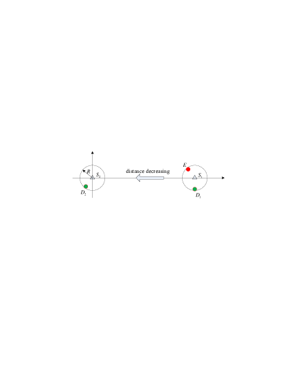
Figure 3: Model used for numerical experiments

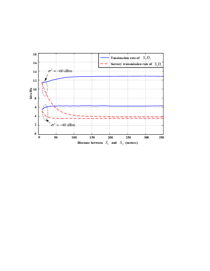
Figure 4: Achievable rates versus $S_{1}$-$S_{2}$ distance

Fig. 4 illustrates the achievable secrecy transmission rate of the user S₁-D₁, and also the achievable transmission rate of the user S₂-D₂ for $N_{1}=4$ and $N_{2}=2$. The noise power $\sigma^{2}=-60$dBm and $\sigma^{2}=-40$dBm are considered, respectively. According to (48), we see that with our proposed cooperative transmission scheme, the S.D.o.F. pair (1,1) can be achieved. We compute the precoding vectors $\bf v$ and $\bf w$ according to TABLE III, and compute the achievable transmission rate of each user according to (7) and (8), respectively. It shows that the achievable secrecy transmission rate of S₁-D₁ increases monotonically as S₁ moves close to S₂. In contrast, the achievable transmission rate of S₂-D₂ decreases with the decreasing of the source-source distance. As compared with the decrease in the transmission rate of S₂-D₂, the increase in the secrecy transmission rate of S₁-D₁ is drastic. Therefore, the network performance benefits when the two users get closer.

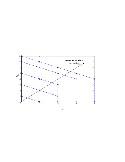
Figure 5: Achievable secrecy degrees of freedom region with an increasing number of antennas at S₂-D₂

Fig. 5 illustrates the achievable secrecy degrees of freedom region versus different values of $N_{2}$. Here, we set $N_{1}=4$ and let $N_{2}$ vary from 1 to 8. We compute the achievable secrecy degrees of freedom region according to (48). As expected, the secrecy degrees of freedom region expands with an increasing $N_{2}$. Note that previous work [36] shows that for the classic wiretap channel with no cooperative helpers the condition to achieve a nonzero S.D.o.F. is $N_{s}^{1}\geq N_{e}+1$. Here although $N_{s}^{1}=N_{e}$, by exploiting the co-channel interference an S.D.o.F. of $N_{s}^{1}$ can be achieved.

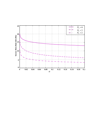
Figure 6: Achievable secrecy rate of S₁-D₁ versus the uncertainty of the eavesdropper’s channels $\alpha$.

In practice, while one may have a good estimate of the position of the eavesdropper, an estimate of the phase of the eavesdropper’s channels is more difficult to obtain. Since the proposed precoding matrix design highly depends on the eavesdropper’s channels, we next examine the secrecy rate performance degradation in the presence of imperfect channel estimate. In Fig. 6, we plot the achievable secrecy rate with imperfect CSI of the eavesdropper’s channels. Here, we set $N_{1}=4$ and let $N_{2}$ vary from 2 to 6. $S_{1}$ and $S_{2}$ are located at (10,0) and (0,0), respectively. The noise power $\sigma^{2}=-60$dBm. The channel from S_i ($i=1,2$) to E is

$${\bf G}_{i}=d_{ei}^{-c/2}\left(\dfrac{1}{\sqrt{1+\alpha}}\bar{\bf G}_{i}+\sqrt{\dfrac{\alpha}{1+\alpha}}\Delta\bar{\bf G}_{i}\right),$$ (61)

where $\alpha$ denotes the channel uncertainty. $\bar{\bf G}_{i}$ represents the estimated channel part at S_i. The entries of $\bar{\bf G}_{i}$ are $e^{j\theta}$ with $\theta$ be a random phase uniformly distributed within $[0,2\pi)$. $\Delta\bar{\bf G}_{i}\sim\mathcal{CN}(\bf{0},\bf{I})$ represents the Gaussian error channel matrices. $d_{ei}$ denotes the distance from S_i. According to (48), we see that the S.D.o.F. pairs (1,1), (2,1) and (3,3) can be achieved for the case of $N_{2}=2$, $N_{2}=3$ and $N_{2}=6$, respectively. For these S.D.o.F. pairs, we construct the precoding matrices $\bf V$ and $\bf W$ according to TABLE III, subject to power being equally allocated between different signal streams. The achievable secrecy transmission rate is computed according to (7). It can be observed that the achievable secrecy rate drops with the increase of channel uncertainties when the channel uncertainty $\alpha$ is small. Fortunately, when the number of antennas $N_{2}$ increases, this secrecy rate performance degradation is smaller. On the other hand, on comparing the secrecy transmission rate of S₁-D₁ for the case $N_{2}=2$ with that in Fig. 4, one can see that the secrecy rate achieved for the case where $\alpha=0.1$ and S₁-S₂ distance of 10 meters, is almost equal to the secrecy rate achieved for the case where $\alpha=0$ and S₁-S₂ distance of 150 meters. This suggests that in wiretap interference networks, the secrecy rate degradation due to CSI estimation error can be counteracted by bringing the two users closer together.

VIII Conclusion

We have examined the maximum achievable secrecy degrees of freedoms (S.D.o.F.) region of a MIMO two-user wiretap interference channel, where one user requires confidential connection against an external passive eavesdropper, while the other uses a public connection. We have addressed analytically the S.D.o.F. pair maximization (component-wise). Specifically, we have proposed a cooperative secrecy transmission scheme and proven that its feasible set is sufficient to achieve all the points on the S.D.o.F. region boundary. For the proposed cooperative secrecy transmission scheme, we have obtained analytically the maximum achievable S.D.o.F. region boundary points. We have also constructed the precoding matrices which achieve the S.D.o.F. region boundary. Our results revealed the connection between the maximum achievable S.D.o.F. region and the number of antennas, thus shedding light on how the secrecy rate region behaves for different number of antennas. Numerical results show that the network performance benefits when the two users get closer. This is interesting. It tells us that in wiretap interference networks, the secrecy rate degradation due to CSI estimation error can be counteracted by bringing the two users closer together.

Appendix A Proof of Proposition 1

In what follows, we prove that ${\bf{A}}{\bf{v}}={\bf{B}}{\bf{w}}$ holds true if and only if $\bf v$ and $\bf w$ are given in (4d) and (4h), with ${\bf{y}}_{s}$, ${\bf{y}}_{s1}$, ${\bf{y}}_{s2}$, ${\bf{y}}_{1}$ and ${\bf{y}}_{2}$ being any vectors with appropriate length. With this result, the first conclusion in Proposition 1 is a natural extension. According to the GSVD decomposition, ${\bf{A}}{\bf\Psi}_{12}{\bf\Lambda}_{1}^{-1}={\bf{B}}{\bf\Psi}_{22}{\bf\Lambda}_{2}^{-1}={\bf X}_{2}$. Thus, ${\bf{A}}{\bf{v}}={\bf{B}}{\bf{w}}$ holds true if ${\bf v}$ and ${\bf w}$ are given by (4d) and (4h), respectively. Next, we prove by contradiction that ${\bf{A}}{\bf{v}}={\bf{B}}{\bf{w}}$ holds true only if ${\bf v}\in{\rm span}({\bf\Phi}_{1})$; the argument for $\bf w$ is similar. Assume that there exists a nonzero vector $\bar{\bf v}\notin{\rm span}({\bf\Phi}_{1})$ satisfying ${\bf{A}}\bar{\bf{v}}={\bf{B}}{\bf{w}}$. Then, ${\bf A}\bar{\bf v}\notin{\rm span}({\bf A}{\bf\Phi}_{1})$; otherwise, it holds that ${\bf A}\bar{\bf v}={\bf A}{\bf\Phi}_{1}{\bf x}$ which implies $\bar{\bf v}-{\bf\Phi}_{1}{\bf x}={\bf\Gamma}({\bf A}){\bf y}_{1}$, and so $\bar{\bf v}\in{\rm span}({\bf\Phi}_{1})$ which contradicts with the assumption. However, ${\bf A}\bar{\bf v}\in{\rm{span}}({\bf X}_{2})$ due to ${\bf{A}}\bar{\bf{v}}={\bf{B}}{\bf{w}}$. In addition, by the GSVD, ${\rm{span}}({\bf X}_{2})={\rm span}({\bf A}{\bf\Phi}_{1})$. Thus, ${\bf A}\bar{\bf v}\in{\rm span}({\bf A}{\bf\Phi}_{1})$ and so ${\bf A}\bar{\bf v}\notin{\rm span}({\bf A}{\bf\Phi}_{1})$ is contradicted. This completes the proof of the first conclusion in Proposition 1.

According to the GSVD, ${\bf{A}}{\bf{\Psi}}_{13}={\bf 0}$. Thus, ${\rm span}({\bf{\Psi}}_{13})\subset{\rm span}({\bf\Gamma}({\bf A}))$. In addition, ${\rm rank}({\bf{\Psi}}_{13})=M-r-s=M-\min\{M,N\}=(M-N)^{+}$, which indicates that the linear independent vectors in ${\rm span}({\bf{\Psi}}_{13})$ is the same as that in ${\rm span}({\bf\Gamma}({\bf A}))$. So, ${\rm span}({\bf{\Psi}}_{13})={\rm span}({\bf\Gamma}({\bf A}))$. Since ${\bf{\Psi}}_{1}$ is an unitary matrix, it holds that ${\rm span}({\bf{\Psi}}_{12})\cap{\rm span}({\bf{\Psi}}_{13})={\bf 0}$. Therefore, ${\rm span}({\bf{\Psi}}_{12})\cap{\rm span}({\bf\Gamma}({\bf A}))={\bf 0}$, which, combined with (4d), indicates that the number of linearly independent vectors $\bf v$ satisfying ${\bf{A}}{\bf{v}}={\bf{B}}{\bf{w}}\neq{\bf 0}$ is $s+{\rm{dim}}\{{\rm{null}}({\bf{A}})\}$. This completes the proof.

Appendix B Proof of Proposition 2

Given an arbitrary point $({\bf V},{\bf W})$, with ${\rm{tr}}\{{\bf Q}_{v}\}=P$ and ${\rm{tr}}\{{\bf Q}_{w}\}=P$. We can respectively rewrite ${\bf Q}_{v}$ and ${\bf Q}_{w}$ as ${\bf Q}_{v}=P\bar{\bf Q}_{v}$ and ${\bf Q}_{w}=P\bar{\bf Q}_{w}$, with ${\rm{tr}}\{\bar{\bf Q}_{v}\}={\rm{tr}}\{{\bar{\bf Q}_{w}}\}=1$. Correspondingly, (9a) can be rewritten as

$$R_{d}^{1}={\rm{log}}|{\bf I}+({\bf I}+P{\bf H}_{12}\bar{\bf Q}_{w}{\bf H}_{12}^{H})^{-1}{\bf H}_{11}\bar{\bf Q}_{v}{\bf H}_{11}^{H}P|.$$ (62)

Let ${\bf\Theta}_{2}={\bf H}_{11}\bar{\bf Q}_{v}{\bf H}_{11}^{H}$. Denoting ${\bf H}_{12}\bar{\bf Q}_{w}{\bf H}_{12}^{H}=\left[{\bf U}_{1}\ {\bf U}_{0}\right]\left[{\begin{array}[]{*{20}{c}}{{{\bf{\Sigma}}_{1}}}&{\bf{0}}\\ {\bf{0}}&{{{\bf{0}}}}\end{array}}\right]\left[{\begin{array}[]{*{20}{c}}{{{\bf{U}}_{1}^{H}}}\\ {{{\bf{U}}_{0}^{H}}}\end{array}}\right]$ as the singular value decomposition (SVD), and substituting it into (62), we obtain

$$R_{d}^{1}= {\rm{log}}|{\bf I}+{\bf U}_{1}({\bf I}+P{\bf\Sigma}_{1})^{-1}{\bf U}_{1}^{H}{\bf\Theta}_{2}P+{\bf U}_{0}{\bf U}_{0}^{H}{\bf\Theta}_{2}P|$$

$$= {\rm{log}}|{\bf I}+{\bf U}_{1}(\frac{\bf I}{P}+{\bf\Sigma}_{1})^{-1}{\bf U}_{1}^{H}{\bf\Theta}_{2}+{\bf U}_{0}{\bf U}_{0}^{H}{\bf\Theta}_{2}P|.$$

Therefore,

$$\lim_{P\to\infty}{R_{d}^{1}}/{{\rm{log}}(P)}$$

$$= \lim_{P\to\infty}\dfrac{{\rm{log}}|{\bf I}+{\bf U}_{1}({\bf\Sigma}_{1})^{-1}{\bf U}_{1}^{H}{\bf\Theta}_{2}+{\bf U}_{0}{\bf U}_{0}^{H}{\bf\Theta}_{2}P|}{{\rm{log}}(P)}$$

$$= \lim_{P\to\infty}\dfrac{{\rm{log}}|{\bf I}+(\frac{1}{P}{\bf U}_{1}({\bf\Sigma}_{1})^{-1}{\bf U}_{1}^{H}+{\bf U}_{0}{\bf U}_{0}^{H}){\bf\Theta}_{2}P|}{{\rm{log}}(P)}$$

$$= \lim_{P\to\infty}\dfrac{{\rm{log}}|{\bf I}+{\bf U}_{0}{\bf U}_{0}^{H}{\bf H}_{11}{\bf V}{\bf V}^{H}{\bf H}_{11}^{H}|}{{\rm{log}}(P)}$$

$$= {\rm{rank}}\{{\bf U}_{0}{\bf U}_{0}^{H}{\bf H}_{11}{\bf V}{\bf V}^{H}{\bf H}_{11}^{H}\}$$ (63)

$$= {\rm{dim}}\{{\rm{span}}({\bf{H}}_{11}{\bf{V}})/{\rm{span}}({\bf{H}}_{12}{\bf{W}})\}$$ (64)

$$= {\rm{rank}}\{{\bf{H}}_{11}{\bf V}\}-{\rm{dim}}\{{\rm{span}}({\bf{H}}_{11}{\bf{V}})\cap{\rm{span}}({\bf{H}}_{12}{\bf{W}})\}.$$ (65)

where (63) comes from the fact that

$$\lim_{P\to\infty}\dfrac{{\rm{log}}|{\bf I}+{\bf A}P|}{{\rm{log}}(P)}=\lim_{P\to\infty}\dfrac{\sum\nolimits_{i=1}^{t}{{\rm{log}}(1+{\lambda_{i}}P)}}{{\rm{log}}(P)}={\rm{rank}}\{\bf A\},$$

with ${\lambda_{i}}$ and $t$ being the nonzero eigenvalue and the rank of ${\bf A}$. (64) comes from the fact that ${\bf U}_{0}{\bf U}_{0}^{H}$ is the projection matrix of the subspace ${\rm{span}}({\bf{H}}_{12}{\bf{W}})^{\perp}$.

Applying similar derivations from (62) to (64) yields

$$\lim_{P\to\infty}\dfrac{R_{d}^{2}}{{\rm{log}}(P)}={\rm{dim}}\{{\rm{span}}({\bf{H}}_{22}{\bf{W}})/{\rm{span}}({\bf{H}}_{21}{\bf{V}})\},$$ (66)

$$\lim_{P\to\infty}\dfrac{R_{e}}{{\rm{log}}(P)}={\rm{dim}}\{{\rm{span}}({\bf{G}}_{1}{\bf{V}})/{\rm{span}}({\bf{G}}_{2}{\bf{W}})\}.$$ (67)

Substituting (65)-(67) into (11), we arrive at (12a) and (12b). This completes the proof.

Appendix C Proof of Proposition 3

By definition, we have $\bar{\mathcal{D}}\subset{\mathcal{D}}$. Thus, the boundary of $\bar{\mathcal{D}}$ is included by that of ${\mathcal{D}}$. In the following, we show that for any given precoding matrices $({\bf V},{\bf W})\in{\mathcal{I}}$, we can always find another precoding matrices $({\bf V}^{\prime},{\bf W}^{\prime})\in\bar{\mathcal{I}}$, which satisfy $d_{s}^{1}({\bf V},{\bf W})\leq d_{s}^{1}({\bf V}^{\prime},{\bf W}^{\prime})$ and $d_{s}^{2}({\bf V},{\bf W})\leq d_{s}^{2}({\bf V}^{\prime},{\bf W}^{\prime})$. So, the boundary of ${\mathcal{D}}$ is included by that of $\bar{\mathcal{D}}$. Concluding, the outer boundary of ${\mathcal{D}}$ is the same as that of $\bar{\mathcal{D}}$.

Before proceeding, we first introduce two critical properties on matrix that will be used in the following analyses. That is, for any given matrices $\bf A$ and $\bf B$, if $\bf B$ is invertible, then

$${\rm{span}}({\bf A})={\rm{span}}({\bf A}{\bf B}),$$ (68)

$${\rm{rank}}\{{\bf A}\}={\rm{rank}}\{{\bf A}{\bf B}\}.$$ (69)

In what follows, based on the GSVD decomposition of $({\bf H}_{12}{\bf W},{\bf H}_{11}{\bf V})$ we first construct a precoding matrix pair $(\hat{\bf V},\hat{\bf W})$, which excludes the intersection subspace of ${\rm{span}}({\bf H}_{12}{\bf W})$ and ${\rm{span}}({\bf H}_{11}{\bf V})$ without decreasing the achieved S.D.o.F. pair. Further, based on the GSVD decomposition of $({\bf G}_{2}\hat{\bf W},{\bf G}_{1}\hat{\bf V})$ we construct a precoding matrix pair $({\bf V}^{\prime},{\bf W}^{\prime})$, which excludes the subspace ${\rm{span}}({\bf G}_{21}\hat{\bf V})/{\rm{span}}({\bf G}_{22}\hat{\bf W})$ without decreasing the achieved S.D.o.F. pair. In this way, we finish the construction of the wanted precoding matrix pair.

Consider the decomposition

$${\rm{GSVD}} ({\bf H}_{12}{\bf W},{\bf H}_{11}{\bf V};N_{d}^{1},K_{w},K_{v})$$

$$=(\hat{\bf\Psi}_{1},\hat{\bf\Psi}_{2},\hat{\bf\Lambda}_{1},\hat{\bf\Lambda}_{2},\hat{\bf X},\hat{k},\hat{r},\hat{s},\hat{p}).$$ (70)

Let $\hat{\bf\Psi}_{2}^{0}=[\hat{\bf\Psi}_{21},\hat{\bf\Psi}_{23}]$. Since $\hat{\bf\Psi}_{1}$ and $\hat{\bf\Psi}_{2}$ are invertible, $\hat{\bf\Psi}_{1}^{\prime}=[\hat{\bf\Psi}_{11},\hat{\bf\Psi}_{13},\hat{\bf\Psi}_{12}]$ and $\hat{\bf\Psi}_{2}^{\prime}=[\hat{\bf\Psi}_{2}^{0},\hat{\bf\Psi}_{22}]$ are also invertible. Applying (68) and (69), we have

$$d_{s}^{1}({\bf V},{\bf W}) =d_{s}^{1}({{\bf V}\hat{\bf\Psi}_{2}^{\prime}},{{\bf W}\hat{\bf\Psi}_{1}^{\prime}})$$ (71a)

$$={\rm{rank}}\{{\bf{H}}_{11}{\bf V}\hat{\bf\Psi}_{2}^{0}\}-m({\bf V}\hat{\bf\Psi}_{2}^{\prime},{\bf W}\hat{\bf\Psi}_{1}^{\prime})$$ (71b)

$$\leq{\rm{rank}}\{{\bf{H}}_{11}{\bf V}\hat{\bf\Psi}_{2}^{0}\}-m({\bf V}\hat{\bf\Psi}_{2}^{0},{\bf W}\hat{\bf\Psi}_{1}^{\prime}),$$ (71c)

in which (71b) can be justified with ${\rm{span(}}{{\bf{H}}_{12}}{\bf{W}}\hat{\bf\Psi}_{1}^{\prime}{\rm{)}}\cap{\rm{span}}({{\bf{H}}_{11}}{\bf{V}}\hat{\bf\Psi}_{2}^{\prime})={\rm{span}}({{\bf{H}}_{11}}{\bf{V}}\hat{\bf\Psi}_{22}$). Besides, (71c) comes from the fact that $m({\bf V}\hat{\bf\Psi}_{2}^{\prime},{\bf W}\hat{\bf\Psi}_{1}^{\prime})\geq m({\bf V}\hat{\bf\Psi}_{2}^{0},{\bf W}\hat{\bf\Psi}_{1}^{\prime})$. Here $({\bf V}\hat{\bf\Psi}_{2}^{0},{\bf W}\hat{\bf\Psi}_{1}^{\prime})$ is the precoding matrix pair $(\hat{\bf V},\hat{\bf W})$ we mentioned in the above text.

Consider the decomposition

$${\rm{GSVD}} ({\bf G}_{2}{\bf W}\hat{\bf\Psi}_{1}^{\prime},{\bf G}_{1}{\bf V}\hat{\bf\Psi}_{2}^{0};N_{e},K_{w},K_{v}-\hat{s})$$

$$=(\breve{\bf\Psi}_{1},\breve{\bf\Psi}_{2},\breve{\bf\Lambda}_{1},\breve{\bf\Lambda}_{2},\breve{\bf X},\breve{k},\breve{r},\breve{s},\breve{p}).$$ (72)

Let $\breve{\bf\Psi}_{2}^{1}=[\breve{\bf\Psi}_{21},\breve{\bf\Psi}_{22}]$. Since $\breve{\bf\Psi}_{1}$ and $\breve{\bf\Psi}_{2}$ are invertible, $\breve{\bf\Psi}_{1}^{\prime}=[\breve{\bf\Psi}_{13},\breve{\bf\Psi}_{11},\breve{\bf\Psi}_{12}]$ and $\breve{\bf\Psi}_{2}^{\prime}=[\breve{\bf\Psi}_{23},\breve{\bf\Psi}_{2}^{1}]$ are also invertible. Applying (68) and (69), we have

$${\rm{rank}}\{{\bf{H}}_{11}{\bf V}\hat{\bf\Psi}_{2}^{0}\}-m({\bf V}\hat{\bf\Psi}_{2}^{0},{\bf W}\hat{\bf\Psi}_{1}^{\prime})$$

$$={\rm{rank}}\{{\bf{H}}_{11}{\bf V}\hat{\bf\Psi}_{2}^{0}\breve{\bf\Psi}_{2}^{\prime}\}-m({\bf V}\hat{\bf\Psi}_{2}^{0}\breve{\bf\Psi}_{2}^{\prime},{\bf W}\hat{\bf\Psi}_{1}^{\prime}\breve{\bf\Psi}_{1}^{\prime})$$ (73a)

$$={\rm{rank}}\{{\bf{H}}_{11}{\bf V}\hat{\bf\Psi}_{2}^{0}\breve{\bf\Psi}_{2}^{\prime}\}-{\rm{rank}}\{\breve{\bf\Psi}_{23}\}$$ (73b)

$$\leq{\rm{rank}}\{{\bf{H}}_{11}{\bf V}\hat{\bf\Psi}_{2}^{0}\breve{\bf\Psi}_{2}^{1}\}.$$ (73c)

Here, since ${\rm{span}}({\bf{G}}_{1}{\bf{V}}\hat{\bf\Psi}_{2}^{0}\breve{\bf\Psi}_{2}^{\prime})/{\rm{span}}({\bf{G}}_{2}{\bf{W}}\hat{\bf\Psi}_{1}^{\prime}\breve{\bf\Psi}_{1}^{\prime})={\rm{span}}({\bf{G}}_{1}{\bf{V}}\hat{\bf\Psi}_{2}^{0}\breve{\bf\Psi}_{23})={\rm{rank}}\{\breve{\bf\Psi}_{23}\}$, we see that (73b) holds true. Since ${\rm{rank}}\{{\bf{H}}_{11}{\bf V}\hat{\bf\Psi}_{2}^{0}\breve{\bf\Psi}_{23}\}\leq{\rm{rank}}\{\breve{\bf\Psi}_{23}\}$ and ${\rm{rank}}\{{\bf{H}}_{11}{\bf V}\hat{\bf\Psi}_{2}^{0}\breve{\bf\Psi}_{2}^{\prime}\}\leq{\rm{rank}}\{{\bf{H}}_{11}{\bf V}\hat{\bf\Psi}_{2}^{0}\breve{\bf\Psi}_{2}^{1}\}+{\rm{rank}}\{{\bf{H}}_{11}{\bf V}\hat{\bf\Psi}_{2}^{0}\breve{\bf\Psi}_{23}\}$, we see that (73c) holds true.

Combining (71a)-(71c) with (73a)-(73c), we arrive at

$$d_{s}^{1}({\bf V},{\bf W})\leq{\rm{rank}}\{{\bf{H}}_{11}{\bf V}\hat{\bf\Psi}_{2}^{0}\breve{\bf\Psi}_{2}^{1}\}.$$ (74)

On the other hand, according to (72), it holds that $m({\bf V}\hat{\bf\Psi}_{2}^{0}\breve{\bf\Psi}_{2}^{1},{\bf W}\hat{\bf\Psi}_{1}^{\prime}\breve{\bf\Psi}_{1}^{\prime})=0$, which indicates

$${\rm{span}}({\bf{G}}_{1}{\bf V}\hat{\bf\Psi}_{2}^{0}\breve{\bf\Psi}_{2}^{1})\subset{\rm{span}}({\bf{G}}_{2}{\bf W}\hat{\bf\Psi}_{1}^{\prime}\breve{\bf\Psi}_{1}^{\prime}).$$ (75)

According to (70), ${\rm{span}}({\bf{H}}_{12}{\bf W}\hat{\bf\Psi}_{1}^{\prime})\cap{\rm{span}}({\bf H}_{11}{\bf V}\hat{\bf\Psi}_{2}^{0})={\bf 0}$, which together with ${\rm{span}}({\bf{H}}_{12}{\bf W}\hat{\bf\Psi}_{1}^{\prime})={\rm{span}}({\bf{H}}_{12}{\bf W}\hat{\bf\Psi}_{1}^{\prime}\breve{\bf\Psi}_{1}^{\prime})$ and ${\rm{span}}({\bf H}_{11}{\bf V}\hat{\bf\Psi}_{2}^{0})\supset{\rm{span}}({\bf H}_{11}{\bf V}\hat{\bf\Psi}_{2}^{0}\breve{\bf\Psi}_{2}^{1})$, implies

$${\rm{span}}({\bf{H}}_{12}{\bf W}\hat{\bf\Psi}_{1}^{\prime}\breve{\bf\Psi}_{1}^{\prime})\cap{\rm{span}}({\bf H}_{11}{\bf V}\hat{\bf\Psi}_{2}^{0}\breve{\bf\Psi}_{2}^{1})={\bf 0}.$$ (76)

Combining (75) and (76), we arrive at

$$({\bf V}\hat{\bf\Psi}_{2}^{0}\breve{\bf\Psi}_{2}^{1},{\bf W}\hat{\bf\Psi}_{1}^{\prime}\breve{\bf\Psi}_{1}^{\prime})\in\bar{\mathcal{I}}.$$ (77)

Let ${\bf V}^{\prime}={\bf V}\hat{\bf\Psi}_{2}^{0}\breve{\bf\Psi}_{2}^{1}$ and ${\bf W}^{\prime}={\bf W}\hat{\bf\Psi}_{1}^{\prime}\breve{\bf\Psi}_{1}^{\prime}$. According to Corollary 2, $d_{s}^{1}({\bf V}^{\prime},{\bf W}^{\prime})={\rm{rank}}\{{\bf{H}}_{11}{\bf V}\hat{\bf\Psi}_{2}^{0}\breve{\bf\Psi}_{2}^{1}\}$, which together with (74), gives $d_{s}^{1}({\bf V},{\bf W})\leq d_{s}^{1}({\bf V}^{\prime},{\bf W}^{\prime})$. Besides, ${\rm{span}}({\bf H}_{21}{\bf V}^{\prime})\subset{\rm{span}}({\bf H}_{21}{\bf V})$ and ${\rm{span}}({\bf H}_{22}{\bf W}^{\prime})={\rm{span}}({\bf H}_{22}{\bf W})$. So $d_{s}^{2}({\bf V},{\bf W})\leq d_{s}^{2}({\bf V}^{\prime},{\bf W}^{\prime})$. This completes the proof.

Appendix D Proof of Corollary 1

Since by definition $\hat{\mathcal{I}}\subset\bar{\mathcal{I}}$, it holds that $\hat{\mathcal{D}}\subset\bar{\mathcal{D}}$. In the sequel, we will show that for any given $({\bf V},{\bf W})\in\bar{\mathcal{I}}$, we can always construct another feasible point $({\bf V}^{\star},{\bf W}^{\star})\in\hat{\mathcal{I}}$, which satisfy $d_{s}^{1}({\bf V}^{\star},{\bf W}^{\star})=d_{s}^{1}({\bf V},{\bf W})$ and $d_{s}^{2}({\bf V}^{\star},{\bf W}^{\star})=d_{s}^{2}({\bf V},{\bf W})$, thus giving the proof of $\hat{\mathcal{D}}\supset\bar{\mathcal{D}}$. Concluding, it holds that $\bar{\mathcal{D}}=\hat{\mathcal{D}}$.

For any given $({\bf V},{\bf W})\in\bar{\mathcal{I}}$, ${\bf V}\in{\mathbb{C}}^{N_{s}^{1}\times K_{v}}$, ${\bf W}\in{\mathbb{C}}^{N_{s}^{2}\times K_{w}}$, we should have $({\bf V},{\bf W})\in\bar{\mathcal{I}}_{1}$ and $({\bf V},{\bf W})\in\bar{\mathcal{I}}_{2}$. Since all channel matrices are assumed to be full rank, it holds that ${\rm{rank}}\{{\bf{G}}_{2}{\bf W}\}=\min\{K_{w},N_{e}\}$.

In the following, we consider two distinct cases.

(i) For the case of $K_{w}\geq N_{e}$, it holds that ${\rm{rank}}\{{\bf{G}}_{2}{\bf W}\}=N_{e}$. Denote ${\bf{G}}_{2}{\bf W}=\left[{\bf U}_{1}\ {\bf U}_{0}\right]\left[{\begin{array}[]{*{20}{c}}{{{\bf{\Sigma}}_{1}}}&{\bf{0}}\\ {\bf{0}}&{{{\bf{0}}}}\end{array}}\right]\left[{\begin{array}[]{*{20}{c}}{{{\bf{T}}_{1}^{H}}}\\ {{{\bf{T}}_{0}^{H}}}\end{array}}\right]$ as the SVD of ${\bf{G}}_{2}{\bf W}$. Then, the matrix ${\bf{G}}_{2}{\bf W}{\bf{T}}_{1}$ is invertible. Let ${\bf B}={\bf{T}}_{1}({\bf{G}}_{2}{\bf{W}}{\bf{T}}_{1})^{-1}{\bf{G}}_{1}{\bf{V}}$. Then,

$${\bf{G}}_{1}{\bf{V}}={\bf{G}}_{2}{\bf{W}}{\bf{T}}_{1}({\bf{G}}_{2}{\bf{W}}{\bf{T}}_{1})^{-1}{\bf{G}}_{1}{\bf{V}}={\bf{G}}_{2}{\bf{W}}{\bf B}.$$ (78)

(ii) For the case of $K_{w}<N_{e}$, ${\bf{G}}_{2}{\bf W}$ is full column rank. Let ${\bf P}$ be the projection matrix of ${\bf{G}}_{2}{\bf{W}}$, i.e.,

$${\bf P}={\bf{G}}_{2}{\bf{W}}(({\bf{G}}_{2}{\bf{W}})^{H}{\bf{G}}_{2}{\bf{W}})^{-1}({\bf{G}}_{2}{\bf{W}})^{H}.$$ (79)

Due to $({\bf V},{\bf W})\in\bar{\mathcal{I}}_{1}$, it holds that

$${\bf{G}}_{1}{\bf{V}} ={\bf P}{\bf{G}}_{1}{\bf{V}}.$$ (80)

Substituting (79) into (80) and letting ${\bf B}=(({\bf{G}}_{2}{\bf{W}})^{H}{\bf{G}}_{2}{\bf{W}})^{-1}({\bf{G}}_{2}{\bf{W}})^{H}{\bf{G}}_{1}{\bf{V}}$, we arrive at

$${\bf{G}}_{1}{\bf{V}}={\bf{G}}_{2}{\bf{W}}{\bf B}.$$ (81)

Let ${\bf V}^{\star}={\bf V}$ and ${\bf W}^{\star}={\bf W}[{\bf B}\ {\bf B}^{\perp}]$. Summarizing the above two cases, for both cases it holds that

$${\bf{G}}_{1}{\bf{V}}^{\star}={\bf{G}}_{2}{\bf{W}}^{\star}(:,1:K_{v}),$$

which, combined with $({\bf V},{\bf W})\in\bar{\mathcal{I}}_{2}$, implies that $({\bf V}^{\star},{\bf W}^{\star})\in\hat{\mathcal{I}}$. On the other hand, since the matrix $[{\bf B}\ {\bf B}^{\perp}]$ is invertible, it holds that $d_{s}^{1}({\bf V}^{\star},{\bf W}^{\star})=d_{s}^{1}({\bf V},{\bf W})$ and $d_{s}^{2}({\bf V}^{\star},{\bf W}^{\star})=d_{s}^{2}({\bf V},{\bf W})$. This completes the proof.

References

- [1] A. D. Wyner, “The wire-tap channel,” Bell Syst. Tech. J., vol. 54, no. 8, pp. 1355–1387, Jan. 1975.
- [2] S. K. Leung-Yan-Cheong and M. E. Hellman, “The Gaussian wire-tap channel,” IEEE Trans. Inf. Theory, vol. 24, no. 4, pp. 451–456, Jul. 1978.
- [3] S. A. A. Fakoorian and A. L. Swindlehurst, “Solutions for the MIMO Gaussian wiretap channel with a cooperative jammer,” IEEE Trans. Signal Process., vol. 59, no. 10, pp. 5013–5022, Oct. 2011.
- [4] L. Li, Z. Chen, and J. Fang, “On secrecy capacity of Gaussian wiretap channel aided by a cooperative jammer,” IEEE Signal Process. Lett., vol. 21, no. 11, pp. 1356–1360, Nov. 2014.
- [5] H.-T. Chiang and J. S. Lehnert, “Optimal cooperative jamming for security,” in Proc. IEEE MILCOM, Baltimore, MD, Nov. 2011, pp. 125–130.
- [6] S. A. A. Fakoorian and A. L. Swindlehurst, “Secrecy capacity of MISO Gaussian wiretap channel with a cooperative jammer,” in Proc. IEEE SPAWC, San Francisco, CA, Jun. 2011, pp. 416–420.
- [7] G. Zheng, I. Krikidis, J. Li, A. P. Petropulu, and B. Ottersten, “Improving physical layer secrecy using full-duplex jamming receivers,” IEEE Trans. Signal Process., vol. 61, no. 20, pp. 4962–4974, Oct. 2013.
- [8] Z. Chu, K. Cumanan, Z. Ding, M. Johnston, and S. Y. Goff, “Secrecy rate optimizations for a MIMO secrecy channel with a cooperative jammer,” IEEE Trans. Veh. Technol., vol. 64, no. 5, pp. 1833–1847, May 2015.
- [9] G. Zheng, L.-C. Choo, and K.-K. Wong, “Optimal cooperative jamming to enhance physical layer security using relays,” IEEE Trans. Signal Process., vol. 59, no. 3, pp. 1317–1322, Mar. 2011.
- [10] J. Li, A. P. Petropulu, and S. Weber, “On cooperative relaying schemes for wireless physical layer security,” IEEE Trans. Signal Process., vol. 59, no. 10, pp. 4985–4997, Oct. 2011.
- [11] L. Dong, Z. Han, A. P. Petropulu, and H. V. Poor, “Improving wireless physical layer security via cooperating relays,” IEEE Trans. Signal Process., vol. 58, no. 3, pp. 1875–1888, Mar. 2010.
- [12] S. Luo, J. Li, and A. P. Petropulu, “Uncoordinated cooperative jamming for secret communications,” IEEE Trans. Inf. Forens. Security, vol. 8, no. 7, pp. 1081–1090, Jul. 2013.
- [13] D. S. Kalogerias, N. Chatzipanagiotis, M. M. Zavlanos, and A. P. Petropulu, “Mobile jammers for secrecy rate maximization in cooperative networks,” in Proc. IEEE ICASSP, Vancouver, Canada, May 2013, pp. 2901–2905.
- [14] J. Wang and A. Swindlehurst, “Cooperative jamming in MIMO ad hoc networks,” in Proc. Asilomar Conf. Signals, Syst. Comput., Pacific Grove, CA, Nov. 2009, pp. 1719–1723.
- [15] J. H. Lee and W. Choi, “Multiuser diversity for secrecy communications using opportunistic jammer selection: secure DoF and jammer scaling law,” IEEE Trans. Signal Process., vol. 62, no. 4, pp. 828–839, Feb. 2014.
- [16] J. Zhu, J. Mo, and M. Tao, “Cooperative secret communication with artificial noise in symmetric interference channel,” vol. 14, no. 10, pp. 885–887, Oct. 2010.
- [17] S. A. A. Fakoorian and A. L. Swindlehurst, “MIMO interference channel with confidential messages: Achievable secrecy rates and precoder design,” IEEE Trans. Inf. Forens. Security, vol. 6, no. 3, pp. 640–649, Sep. 2011.
- [18] O. O. Koyluoglu and H. E. Gamal, “Cooperative encoding for secrecy in interference channels,” IEEE Trans. Inf. Theory, vol. 57, no. 9, pp. 5682–5694, Sep. 2011.
- [19] J. Xie and S. Ulukus, “Secure degrees of freedom of K-User Gaussian interference channels: A unified view,” IEEE Trans. Inf. Theory, vol. 61, no. 5, pp. 2647–2661, May 2015.
- [20] ——, “Secure degrees of freedom region of the Gaussian interference channel with secrecy constraints,” in Proc. IEEE ITW, Hobart, Tasmania, Australia, Nov. 2014, pp. 361–365.
- [21] O. O. Koyluoglu, H. E. Gamal, L. Lai, and H. V. Poor, “Interference alignment for secrecy,” IEEE Trans. Inf. Theory, vol. 57, no. 6, pp. 3323–3332, Jun. 2011.
- [22] T. T. Vu, H. H. Kha, T. Q. Duong, and N.-S. Vo, “On the interference alignment designs for secure multiuser MIMO systems,” [online], Available: http://arxiv.org/abs/1508.00349.
- [23] A. Kalantari, S. Maleki, G. Zheng, S. Chatzinotas, and B. Ottersten, “Joint power control in wiretap interference channels,” IEEE Trans. Wireless Commun., vol. 14, no. 7, pp. 3810–3823, Jul. 2015.
- [24] T. Lv, H. Gao, and S. Yang, “Secrecy transmit beamforming for heterogeneous networks,” IEEE J. Sel. Areas Commun., vol. 33, no. 6, pp. 1154–1170, Jun. 2015.
- [25] M. Nafea and A. Yener, “How many antennas does a cooperative jammer need for achieving the degrees of freedom of multiple antenna Gaussian channels in the presence of an eavesdropper?” in Proc. Allerton Conf., Allerton House, UIUC, Illinois, USA, Oct. 2013, pp. 774–780.
- [26] ——, “Secure degrees of freedom for the MIMO wiretap channel with a multiantenna cooperative jammer,” in Proc. IEEE ITW, Hobart, Australia, Nov. 2014, pp. 626–630.
- [27] ——, “Secure degrees of freedom of -- wiretap channel with a -antenna cooperative jammer,” in Proc. IEEE ICC, London, United Kingdom, Jun. 2015, pp. 4169–4174.
- [28] A. Agustin and J. Vidal, “Improved interference alignment precoding for the MIMO channel,” in Proc. IEEE ICC, Kyoto, Japan, Jun. 2011, pp. 1–5.
- [29] T. Gou and S. A. Jafar, “Degrees of freedom of the -user MIMO interference channel,” IEEE Trans. Inf. Theory, vol. 56, no. 12, pp. 6040–6057, Dec. 2010.
- [30] C. M. Yetis, T. Gou, S. A. Jafar, and A. H. Kayran, “On feasibility of interference alignment in MIMO interference networks,” IEEE Trans. Signal Process., vol. 58, no. 9, pp. 4771–4782, Sep. 2010.
- [31] J. Chen, Q. T. Zhang, and G. Chen, “Joint space decomposition-and-synthesis approach and achievable DoF regions for -user MIMO interference channels,” IEEE Trans. Signal Process., vol. 62, no. 9, pp. 2304–2316, May 2014.
- [32] C. Paige and M. A. Saunders, “Towards a generalized singular value decomposition,” SIAM J. Numer. Anal., vol. 18, no. 3, pp. 398–405, Jun. 1981.
- [33] T. Liu and S. Shamai (Shitz), “A note on the secrecy capacity of the multi-antenna wire-tap channel,” IEEE Trans. Inf. Theory, vol. 55, no. 6, pp. 2547–2553, Jun. 2009.
- [34] R. Liu, T. Liu, H. V. Poor, and S. Shamai (Shitz), “Multiple-input multiple-output Gaussian broadcast channels with confidential messages,” IEEE Trans. Inf. Theory, vol. 56, no. 9, pp. 4215–4227, Sep. 2010.
- [35] F. Oggier and B. Hassibi, “The secrecy capacity of the MIMO wiretap channel,” IEEE Trans. Inf. Theory, vol. 57, no. 8, pp. 4961–4971, Aug. 2011.
- [36] A. Khisti and G. Wornell, “Secure transmission with multiple antennas-II: the MIMOME wiretap channel,” IEEE Trans. Inf. Theory, vol. 56, no. 11, pp. 5515–5532, Nov. 2010.