Generating Realistic Synthetic Population Datasets

Abstract

Modern studies of societal phenomena rely on the availability of large datasets capturing attributes and activities of synthetic, city-level, populations. For instance, in epidemiology, synthetic population datasets are necessary to study disease propagation and intervention measures before implementation. In social science, synthetic population datasets are needed to understand how policy decisions might affect preferences and behaviors of individuals. In public health, synthetic population datasets are necessary to capture diagnostic and procedural characteristics of patient records without violating confidentialities of individuals. To generate such datasets over a large set of categorical variables, we propose the use of the maximum entropy principle to formalize a generative model such that in a statistically well-founded way we can optimally utilize given prior information about the data, and are unbiased otherwise. An efficient inference algorithm is designed to estimate the maximum entropy model, and we demonstrate how our approach is adept at estimating underlying data distributions. We evaluate this approach against both simulated data and on US census datasets, and demonstrate its feasibility using an epidemic simulation application.

1 introduction

Many research areas, e.g., epidemiology, public health, social science, study the behavior of large populations of individuals under natural scenarios as well as under human interventions. A key need across these domains is the ready availability of realistic synthetic datasets that can capture key attributes and activities of large populations.

For instance, in epidemiology, synthetic populations are necessary to study disease propagation and intervention measures before implementation. Information from the US census is typically used to model such synthetic datasets. In social science, synthetic populations are necessary to understand how policy decisions might affect preferences and behaviors of individuals. Finally, in public health, synthetic populations are necessary to capture diagnostic and procedural characteristics of patient records without violating confidentialities of individuals.

Typically, the constraints underlying synthetic population generation are assumptions on the supporting marginal or conditional distributions. Although there exist prior research in estimating probability distributions subject to constraints (e.g., Monte Carlo methods), they are primarily focused on continuous-valued data. Many domains on the other hand, such as those studied here, feature the need for multi-dimensional categorical datasets.

As a case in point, in epidemiology, one important task is to simulate disease spread and potential outbreaks on the city- or nation-level, and provide useful information to public health officials to support policy and decision making. To make such simulations as accurate as possible, synthetic populations that have the same structural and behavioral properties as the real population are needed. In domains like health care, privacy is an additional issue motivating the design of synthetic populations. In these applications, the necessary datasets to be generated can be represented as tuples with categorical data attributes.

Motivated by these emerging needs, we focus our attention on constructing a generative model that captures given characteristics of categorical population attributes, and best estimates the underlying data generation distribution. However, modeling multi-dimensional categorical data and estimating distributions can be quite challenging due to the exponential possibilities of data spaces in terms of the number of dimensions of categorical data tuples. To address these challenges and difficulties, we take the first step here to study this problem. To model categorical data with statistical constraints, we apply the classical and statistically well-founded maximum entropy model. We construct a generative maximum entropy model wherein the probabilities of certain categorical patterns are required to satisfy given constraints. In this way, the maximum entropy model maintains the selected characteristics of the underlying categorical data distribution. By sampling the categorical tuples from the maximum entropy model, synthetic population datasets can be generated.

Figure 1: Process of generating realistic synthetic data with our proposed approach.

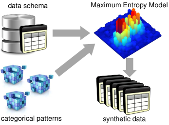
Generally, solving maximum entropy models can be infeasible in practice. In this paper, we show that by leveraging the structure of the categorical data space in our setting, the maximum entropy model could be inferred quite efficiently. We also propose a heuristic together with the Bayesian information criterion (BIC) to select a simple as well as an informative model. To summarize our approach in a nutshell, our contributions are:

1. We formalize the problem of generating synthetic population datasets via a generative maximum entropy model for categorical data, which captures the statistical features of the underlying categorical data distributions.

2. By exploring the structure of the categorical data space, we propose a partition scheme to make the maximum entropy model inference more efficient than the general case. We also present an efficient graph-based model inference algorithm.

3. We propose a BIC-based heuristic to perform model selection wherein the simple and informative maximum entropy model will be chosen.

4. Using results on both synthetic datasets and real US census data, we demonstrate that the proposed maximum entropy model is capable of recovering the underlying categorical data distribution and generating relevant synthetic populations.

2 Preliminaries

Let $\mathcal{A}=\{A_{1},A_{2},\ldots,A_{q}\}$ denote a set of categorical random variables (or attributes), and $\mathcal{R}(A_{i})=\{a_{1}^{(i)},a_{2}^{(i)},\ldots,a_{k_{i}}^{(i)}\}$ represent the set of $k_{i}$ possible values for random variable $A_{i}$. Here, $|\cdot|$, e.g. $|\mathcal{R}(A_{i})|$, is used to represent the cardinality of a set.

By a random categorical tuple, we mean a vector of categorical random variables, e.g. $T=(A_{1},A_{2},\ldots,A_{q})$, which is generated by some unknown probability distribution. The notation of $T(A_{i})$ is used to represent the value of attribute $A_{i}$ in tuple $T$. The space of all the possible categorical tuples is denoted by $\mathcal{S}=\prod_{i=1}^{q}\mathcal{R}(A_{i})$, where $\prod\cdot$ is the series of Cartesian product over the given sets. Given a categorical pattern, which is defined as an ordered set $X=(A_{i}\mid A_{i}\in C,C\subseteq\mathcal{A})$ over a subset of random variables $C\subseteq\mathcal{A}$, let $\mathcal{S}_{X}=\prod_{A_{i}\in C}\mathcal{R}(A_{i})$ represent the space that contains all the possible values of pattern $X$. An instantiation of pattern $X$ is defined as $\boldsymbol{x}=\left(a_{j}^{(i)}\mid a_{j}^{(i)}\in\mathcal{R}(A_{i}),A_{i}\in C,C\subseteq\mathcal{A}\right)$, and $X(A_{i})$ is used to represent the value of attribute $A_{i}$ in the pattern $X$.

For any pattern value $\boldsymbol{x}$ associated with pattern $X$, we use the notation of $T=\boldsymbol{x}$ if the corresponding random variables in $T$ equal to the values in $\boldsymbol{x}$ and $p(T=\boldsymbol{x})$ to denote the probability of $T=\boldsymbol{x}$. Given a categorical dataset $D$, $\tilde{p}(T=\boldsymbol{x}\mid D)$ is used to denote the empirical probability of $T=\boldsymbol{x}$ in the dataset $D$. An indicator function $I_{X}(T=\boldsymbol{x}):\mathcal{S}\rightarrow\{0,1\}$ of pattern $X$, which maps a categorical tuple to a binary value, is defined as:

$$I_{X}(T=\boldsymbol{x})=\left\{\begin{array}[]{l}1,\quad\text{if}~{}T=\boldsymbol{x},\\ 0,\quad\text{otherwise}.\end{array}\right.$$

Given a probability distribution $p$ over the categorical tuple space $\mathcal{S}$, the entropy $H(p)$ with respect to $p$ is defined as:

$$H(p)=-\sum_{T\in{}\mathcal{S}}p(T)\log{p(T)}~{}.$$

The Maximum Entropy principle states that among a set of probability distributions $\mathcal{P}$ that comply with the given prior information about the data, the maximum entropy distribution

$$p^{*}=\operatornamewithlimits{argmax}_{p\in{}\mathcal{P}}H(p)$$

will optimally use the current prior information and best summarize the data. Otherwise, it is fully unbiased.

Problem Statement

Given a set of categorical patterns $\mathcal{X}$ with associated empirical frequencies as the prior information of a dataset, we would like to find a probabilistic model $p$ that best utilizes such prior information and helps to regenerate categorical datasets that conform to the given prior information.

3 Categorical Maximum Entropy model

3.1 Categorical MaxEnt Model Specification

Suppose we have a set categorical patterns $\mathcal{X}=\{X_{i}\mid i=1,2,\ldots,n\}$ and an associated set of empirical probabilities $\tilde{P}=\{\tilde{p}(T=\boldsymbol{x}_{i,j}\mid D)\mid\boldsymbol{x}_{i,j}\in{}\mathcal{S}_{X_{i}},i=1,2,\ldots,n\}$ as prior information about dataset $D$. Here, $\boldsymbol{x}_{i,j}$ denotes the $j^{th}$ value of the pattern $X_{i}$. Notice that it is not necessary that every possible value of pattern $X_{i}$ in $\mathcal{S}_{X_{i}}$ is provided as part of the prior information here. Such prior information identifies a group of probability distributions $\mathcal{P}$ over $\mathcal{S}$ which agree with the empirical probabilities of the given categorical patterns. That is:

$$\mathcal{P} =\{p\}~{}\text{s.t.}~{}p(T=\boldsymbol{x}_{i,j})=\tilde{p}(T=\boldsymbol{x}_{i,j}\mid D),$$ (1)

$$\forall p\in\mathcal{P},X_{i}\in\mathcal{X},~{}\text{and}~{}\tilde{p}(T=\boldsymbol{x}_{i,j}\mid D)\in\tilde{P}$$

Following the Maximum Entropy principle, for all $p\in{}\mathcal{P}$, we are particularly interested in the Maximum Entropy distribution which optimally represents the given prior information. The famous theorem in [5] (Theorem 3.1) shows that the Maximum Entropy distribution has an exponential form. In our categorical scenario, the Maximum Entropy distribution could be written as

$$p^{*}(T)=u_{0}\prod_{X_{i}\in{}\mathcal{X}}\prod_{\boldsymbol{x}_{i,j}\in\mathcal{S}_{X_{i}}}{\left(u_{i,j}\right)}^{I_{X_{i}}(T=\boldsymbol{x}_{i,j})}~{},$$ (2)

where $u_{i,j}\in\mathbb{R}$ are the model parameters associated with each model constraint specified in Equation (1), and $u_{0}$ is the normalizing constant.

3.2 Incorporating Individual Attribute Frequ-encies

The frequencies of individual attributes play an important role in the pattern analysis and discovery. Such frequencies characterize the attribute marginal distributions which convey basic information about the data currently under investigation, and yet are relatively easy to calculate from the data. Incorporating such individual attribute frequencies will enrich the categorical Maximum Entropy model, and make it more informative.

Although such individual attribute frequencies can be trea-ted as part of the categorical pattern set $\mathcal{X}$, considering the computation efficiency which will be explained in detail in the next section, the categorical Maximum Entropy model treats them separately. Let $v_{i,j}$ denote the model parameters corresponding to the individual attribute model constraints, then, the Maximum Entropy distribution can be factorized as:

$$p^{*}(T)=u_{0}\prod_{X_{i}\in{}\mathcal{X}}\prod_{\boldsymbol{x}_{i,j}\in\mathcal{S}_{X_{i}}}{\left(u_{i,j}\right)}^{I_{X_{i}}(T=\boldsymbol{x}_{i,j})}\times\prod_{A_{i}\in{}\mathcal{A}}\prod_{a_{j}\in{}\mathcal{R}(A_{i})}{\left(v_{i,j}\right)}^{I_{A_{i}}(T=a_{j})}~{}.$$ (3)

Notice that the second component involved with $v_{i,j}$ also follows the exponential form described in Equation (2). By introducing a normalizing constant $v_{0}$, an independent Maximum Entropy distribution $p_{\mathcal{A}}(T)$ that only involves individual attribute constraints could be defined as:

$$p_{\mathcal{A}}(T)=v_{0}\prod_{A_{i}\in{}\mathcal{A}}\prod_{a_{j}\in{}\mathcal{R}(A_{i})}{\left(v_{i,j}\right)}^{I_{A_{i}}(T=a_{j})}~{}.$$ (4)

Combining Equation (3) and (4), the Maximum Entropy distribution that incorporates individual attribute frequencies would be specified as:

$$p^{*}(T)=p_{\mathcal{A}}(T)\frac{u_{0}}{v_{0}}\prod_{X_{i}\in{}\mathcal{X}} \prod_{\boldsymbol{x}_{i,j}\in\mathcal{S}_{X_{i}}}{\left(u_{i,j}\right)}^{I_{X_{i}}(T=\boldsymbol{x}_{i,j})}~{}.$$ (5)

4 Model Inference

In this section, we develop an efficient algorithm to infer the categorical Maximum Entropy model. Our algorithm is built on the well-known Iterative Scaling [6] framework. The general idea of the algorithm is that starting from the uniform distribution, it iteratively updates each model parameter to make the distribution satisfy the corresponding constraint until it converges to the Maximum Entropy distribution.

4.1 Efficient Model Inference

The main challenge in the Iterative Scaling framework is how to efficiently query the Maximum Entropy model during the iterative updates of the model parameters. In order to achieve that, we need to explore the particular structure of the tuple space $\mathcal{S}$ determined by the given pattern set $\mathcal{X}$. After examining the exponential form of the Maximum Entropy distribution in Equation (2), we observe that for any two categorical tuples $T_{1}$ and $T_{2}$ in $\mathcal{S}$, if they contain the same subset of categorical patterns in $\mathcal{X}$, they will have the same probability under the Maximum Entropy distribution inferred $\mathcal{X}$. In another word, $\forall T_{1},T_{2}\in\mathcal{S}$, if $I_{X_{i}}(T_{1}=\boldsymbol{x}_{i,j})=I_{X_{i}}(T_{2}=\boldsymbol{x}_{i,j})$ holds true for all $X_{i}\in\mathcal{X}$ and $\tilde{p}(T=\boldsymbol{x}_{i,j}\mid D)\in\tilde{P}$, then $p^{*}(T_{1})=p^{*}(T_{2})$. Based on such observation, we have the following definition of tuple block.

Definition 1.

A tuple block $B$ is a set categorical tuples such that $\forall T_{1},T_{2}\in B$, $I_{X_{i}}(T_{1}=\boldsymbol{x}_{i,j})=I_{X_{i}}(T_{2}=\boldsymbol{x}_{i,j})$ holds true for all $X_{i}\in\mathcal{X}$, $\boldsymbol{x}_{i,j}\in\mathcal{S}_{X_{i}},and~{}\tilde{p}(T=\boldsymbol{x}_{i,j}\mid D)\in\tilde{P}$.

With the definition of tuple block, we could partition the entire categorical tuple space into several tuple blocks. When $|\mathcal{X}|\ll|\mathcal{A}|$, the partition scheme introduced here could greatly reduce the dimensionality of the space we are working on. Here, we use $\mathcal{B}_{\mathcal{X}}$ to denote the tuple block space generated based on pattern set $\mathcal{X}$. Also, the definition of tuple block let us extend the indicator function defined over tuple space to the domain of tuple block, which is defined as:

$$I_{X_{i}}(B\mid\boldsymbol{x}_{i,j})=I_{X_{i}}(T=\boldsymbol{x}_{i,j}),\quad\forall X_{i}\in\mathcal{X},T\in B.$$

1

input : A set of categorical patterns $\mathcal{X}$, and associated empirical probabilities $\tilde{P}$.

output : tuple block graph $G$.

2

3Let $G\leftarrow\{\varnothing\}$;

4 foreach $X_{i}\in\mathcal{X},\boldsymbol{x}_{i,j}\in\mathcal{S}_{X_{i}}~{}s.t.~{}\tilde{p}(T=\boldsymbol{x}_{i,j})\in\tilde{P}$ do

5       foreach $B_{k}\in G$ do

6             $B_{\mathit{new}}\leftarrow$ createBlock($B_{k},X_{i}$);

7             if $B_{\mathit{new}}\neq\mathit{Null}$ then

8                   findPosition($\varnothing$, Null, $B_{\mathit{new}}$);

9                  

10             end if

11            

12       end foreach

13      

14 end foreach

15return $G$;

Algorithm 1 Constructing tuple Block Graph

1

input : Current block $B_{\mathit{curr}}$, last visited block $B_{\mathit{last}}$, new block $B_{\mathit{new}}$.

output : Success or Fail.

2

3if $B_{\mathit{new}}$ and $B_{\mathit{curr}}$ are the same then

4       return Success;

5      

6 else if $B_{\mathit{new}}\subseteq B_{\mathit{\mathit{curr}}}$ then

7       $\mathit{child}(B_{\mathit{last}})\leftarrow\mathit{child}(B_{\mathit{last}})\setminus\{B_{\mathit{curr}}\}$;

8       $\mathit{child}(B_{\mathit{new}})\leftarrow\mathit{child}(B_{\mathit{new}})\cup\{B_{\mathit{curr}}\}$;

9       $\mathit{child}(B_{\mathit{last}})\leftarrow\mathit{child}(B_{\mathit{last}})\cup\{B_{\mathit{new}}\}$;

10       return Success;

11      

12 else if $B_{\mathit{curr}}\subseteq B_{\mathit{new}}$ then

13       if $\mathit{child}(B_{\mathit{curr}})=\emptyset$ then

14             $\mathit{child}(B_{\mathit{curr}})\leftarrow\mathit{child}(B_{\mathit{curr}})\cup\{B_{\mathit{new}}\}$;

15             return Success;

16            

17      else

18             $\mathit{failBlock}\leftarrow$ InsertDescendant($B_{\mathit{new}}$, $B_{\mathit{curr}}$);

19             checkDescendant($\mathit{failBlock}$, $B_{\mathit{new}}$);

20             return Success;

21            

22      

23 return Fail;

24 Procedure InsertDescendant($B_{\mathit{new}}$, $B_{\mathit{curr}}$):

25       $\mathit{failBlock}\leftarrow\emptyset$, $\mathit{accu}\leftarrow$ Fail;

26       foreach $B_{k}\in\mathit{child}(B_{\mathit{curr}})$ do

27             $r\leftarrow$ findPosition($B_{k}$, $B_{\mathit{curr}}$, $B_{\mathit{new}}$);

28             if $r=$ Success then

29                   $\mathit{accu}\leftarrow$ Success;

30                  

31            else

32                   $\mathit{failBlock}\leftarrow\mathit{failBlock}\cup\{B_{k}\}$;

33                  

34            

35       end foreach

36      if $\mathit{accu}=$ Fail then

37             $\mathit{child}(B_{\mathit{curr}})\leftarrow\mathit{child}(B_{\mathit{curr}})\cup\{B_{\mathit{new}}\}$;

38            

39       return $\mathit{failBlock}$;

40      

41

42

Algorithm 2 findPosition procedure

By introducing tuple blocks, we transfer the problem of computing categorical pattern probability $p(T=\boldsymbol{x}_{i,j})$ on tuple space to the block space, which makes it possible to calculate $p(T=\boldsymbol{x}_{i,j})$ in a reasonable time. In the context of tuple blocks, the pattern probability $p(T=\boldsymbol{x}_{i,j})$ in would be

$$p(T=\boldsymbol{x}_{i,j})=\sum_{\begin{subarray}{c}B\in\mathcal{B}_{\mathcal{X}},\\ I_{X_{i}}(B\mid\boldsymbol{x}_{i,j})=1\end{subarray}}p(B)~{},$$

where $p(B)$ is the probability for tuple block $B$. Since the probabilities for the categorical tuples within the same block are all the same, the probability for the tuple block $B$ is defined as:

$$p(B)=\sum_{T\in B}p(T)=|B|\times u_{0}\prod_{X_{i}\in\mathcal{X}}\prod_{\boldsymbol{x}_{i,j}\in\mathcal{S}_{X_{i}}}(u_{i,j})^{I_{X_{i}}(B\mid\boldsymbol{x}_{i,j})}~{}.$$

Now, our problem comes down to how to organize the tuple block space $\mathcal{B}_{\mathcal{X}}$ and efficiently compute the number of categorical tuples in each block, or in other words, the size $|B|$ of each tuple block $B$. In order to achieve that, we introduce a partial order on $\mathcal{B}_{\mathcal{X}}$. Let

$$\mathit{attr}(B)=\bigcup_{\begin{subarray}{c}X_{i}\in\mathcal{X},\\ I_{X_{i}}(B\mid\boldsymbol{x}_{i,j})=1\end{subarray}}X_{i}~{},$$

which represents the set of attributes involved by tuple block $B$. Then, we have the definition about the partial order over $\mathcal{B}_{\mathcal{X}}$ as described below.

Definition 2.

Given any tuple blocks $B_{1},B_{2}\in\mathcal{B}_{\mathcal{X}}$, $B_{1}\subseteq B_{2}$ if and only if the following conditions hold true:

1. $\mathit{attr}(B_{1})\subseteq\mathit{attr}(B_{2})$;

2. $B_{1}(A_{k})=B_{2}(A_{k}),~{}\forall A_{k}\in\mathit{attr}(B_{1})\cap\mathit{attr}(B_{2})$.

Here, $B(A_{k})$ denotes the value of attribute $A_{k}$ in the tuple block $B$. It is easy to verify that Definition 2 satisfies the property of reflexivity, antisymmetry and transitivity.

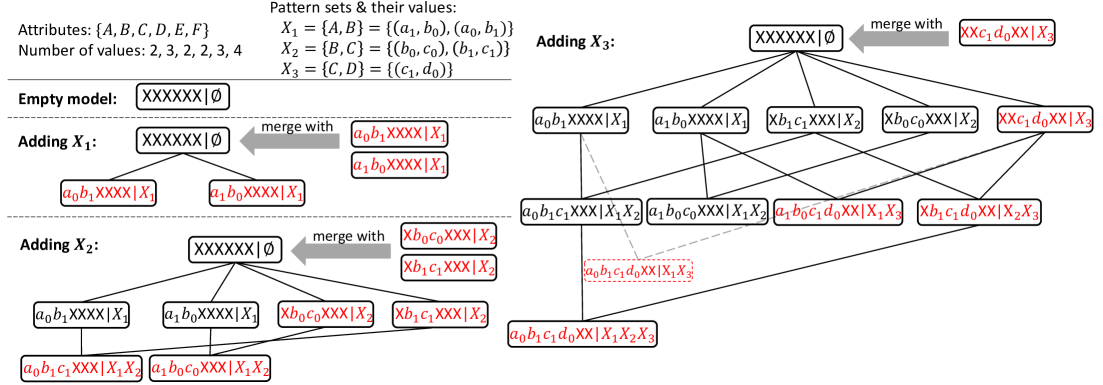
With the partial order $\subseteq$ defined on $\mathcal{B}_{\mathcal{X}}$ here, it is natural to organize the tuple blocks into a hierarchical graph structure. That is, if tuple block $B_{k}\subseteq B_{l}$, block $B_{l}$ is organized as the child of block $B_{k}$. Algorithm 1 illustrates how such block graph is constructed and maintained. The algorithm starts with the graph that has only one block represented by $\varnothing$ indicating that none of the categorical patterns is involved in this block (line 1). We will refer this block as root block in the rest of this section. Then, for each of the pattern set $X_{i}\in\mathcal{X}$ and its possible value $\boldsymbol{x}_{i,j}$, we attempt to create a new tuple block by merging it with every existing block $B_{k}$ from root level to leaf level (without child blocks) in the current block graph $G$ if they are compatible (line 1). A categorical pattern $X_{i}$ is not compatible with tuple block $B_{k}$ if $\mathit{attr}(B_{k})\cap X_{i}\neq\emptyset$, and $\exists A_{i}\in\mathit{attr}(B_{k})\cap X_{i}$ such that $B_{k}(A_{i})\neq X_{i}(A_{i})$. If a new tuple block $B_{\mathit{new}}$ is created, it is obvious that for all $X_{l}\in\mathcal{X},I_{X_{l}}(B_{k}\mid\boldsymbol{x}_{l,j})=1$, we have $I_{X_{l}}(B_{\mathit{new}}\mid\boldsymbol{x}_{l,j})=1$ and also $I_{X_{i}}(B_{\mathit{new}}\mid\boldsymbol{x}_{i,j})=1$. Finally, the new tuple block $B_{\mathit{new}}$ will be added into the current block graph $G$ based on the partial order described in Definition 2 (line 1).

To be more specific, Algorithm 2 illustrates how the procedure findPosition inserts a new tuple block into the block graph $G$ in a recursive manner. Depending on the relationship between the current block $B_{\mathit{curr}}$ we are visiting and the new block $B_{\mathit{new}}$, the insertion operation could be classified into four scenarios.

Figure 2: Example of constructing tuple block graph on toy dataset with 6 attributes and 3 categorical patterns. The blocks marked with red denote the new tuple blocks created in each iteration by adding new categorical patterns.

Case 1: $B_{\mathit{new}}$ and $B_{\mathit{curr}}$ are the same tuple block. Two tuple block $B_{k}$ and $B_{l}$ are considered to be the same if they cover the same set of categorical patterns, e.g. $\forall X_{i}\in\mathcal{X},\boldsymbol{x}_{i,j}\in\mathcal{S}_{X_{i}}~{}s.t.~{}\tilde{p}(T=\boldsymbol{x}_{i,j})\in\tilde{P}$, we have $I_{X_{i}}(B_{k}\mid\boldsymbol{x}_{i,j})=I_{X_{i}}(B_{l}\mid\boldsymbol{x}_{i,j})$. Since block $B_{\mathit{new}}$ and $B_{\mathit{curr}}$ are the same and $B_{\mathit{curr}}$ is already part of the block graph, inserting $B_{\mathit{new}}$ into block graph is not necessary any more. Thus, we simply return Success in this scenario (line 2 – 2).

Case 2: $B_{\mathit{new}}\subseteq B_{\mathit{curr}}$. In this case, the new tuple block $B_{\mathit{new}}$ should be inserted between block $B_{\mathit{last}}$ and $B_{\mathit{curr}}$. To achieve this, block $B_{\mathit{curr}}$ is first removed from the child block set of $B_{\mathit{last}}$, and added as the child block of $B_{\mathit{new}}$. Finally, the new block $B_{\mathit{new}}$ is inserted as the child block of $B_{\mathit{last}}$, and Success is returned (line 2 – 2).

Case 3: $B_{\mathit{curr}}\subseteq B_{\mathit{new}}$. In this scenario, the new tuple block $B_{\mathit{new}}$ should be inserted as a descendant of the current block $B_{\mathit{curr}}$. Depending on whether the block $B_{\mathit{curr}}$ has any child blocks, the insertion operation can be further divided into two sub-cases:

• Case 3.1: block $B_{\mathit{curr}}$ has no child block. In this scenario, the new block $B_{\mathit{new}}$ is directly inserted as the new child of $B_{\mathit{curr}}$ (line 2 – 2);

• Case 3.2: block $B_{\mathit{curr}}$ has child blocks. Then, for each child block of $B_{\mathit{curr}}$, the findPosition procedure is recursively performed to find the correct position to insert block $B_{\mathit{new}}$ (line 2 – 2). If none of these operations succeeds, block $B_{\mathit{new}}$ will be inserted as a new child block of $B_{\mathit{curr}}$ (line 2 – 2). At last, the descendants of the child blocks of $B_{\mathit{curr}}$ on which the findPosition procedure failed to insert the block $B_{\mathit{new}}$ are further examined to see whether any of them would satisfy the partial order with block $B_{\mathit{new}}$ and be added as the child block of $B_{\mathit{new}}$ (line 2).

Case 4: $B_{\mathit{new}}$ does not have any particular relationship with $B_{\mathit{curr}}$. In this case, nothing needs to done with the tuple blocks $B_{\mathit{curr}}$ and $B_{\mathit{new}}$, and Fail is simply returned to indicate that the attempt to insert block $B_{\mathit{new}}$ is failed.

Figure 2 shows an example of constructing such hierarchical block graph on a small toy dataset with 6 attributes and 3 categorical patterns. With the block graph $G$, the size of the tuple block could be easily calculated using the set inclusion-exclusion principle. We first define the cumulative size of a tuple block $B$, which is given by

$$\mathit{cum}(B)=\prod_{A_{i}\in\mathcal{A}\setminus\mathit{attr}(B)}|\mathcal{R}(A_{i})|~{}.$$

Then the actual block size for block $B$ could be computed as

$$|B|=\mathit{cum}(B)-\sum_{B_{k}\in\mathcal{B}_{\mathcal{X}},B\subseteq B_{k}}|B_{k}|~{}.$$

In the block graph $G$, the tuple blocks that satisfy $B_{k}\in\mathcal{B}_{\mathcal{X}},B\subseteq B_{k}$ are simply those descendant blocks of $B$. Algorithm 3 describes the procedure of computing block size for each tuple block in $\mathcal{B}_{\mathcal{X}}$ with the block graph $G$, where $\mathit{desc}(B)$ represents the set of descendant blocks of $B$ in the graph $G$.

1

input : tuple block graph $G$, current visited block $B_{\mathit{curr}}$.

output : Block size for each $B\in\mathcal{B}_{\mathcal{X}}$.

2

3$\mathit{cum}(B_{\mathit{curr}})\leftarrow\prod\limits_{A_{i}\in\mathcal{A}\setminus\mathit{attr}(B_{\mathit{curr}})}|\mathcal{R}(A_{i})|$;

4 if $\mathit{child}(B_{\mathit{curr}})=\emptyset$ then

5       $|B_{\mathit{curr}}|\leftarrow\mathit{cum}(B_{\mathit{curr}})$;

6       return ;

7      

8 end if

9foreach $B_{k}\in\mathit{child}(B_{\mathit{curr}})$ do

10       computeBlockSize($G$, $B_{k}$);

11      

12 end foreach

13$|B_{\mathit{curr}}|\leftarrow\mathit{cum}(B_{\mathit{curr}})-\sum\limits_{B_{k}\in\mathit{desc}(B_{\mathit{curr}})}|B_{k}|$;

14 return ;

15

Algorithm 3 computeBlockSize procedure

When individual attribute constraints are taken into account, the problem become a little more complicated. However, it is obviously not feasible to combine the individual attribute constraints with the categorical pattern constraints together and construct the tuple block graph. This will make the tuple block space blow up. Instead, as we mentioned previously in Section 3.2, the individual attribute constraints are modeled with a separate Maximum Entropy distribution $p_{\mathcal{A}}$, defined in Equation (4), which only considers these constraints. The block graph $G$ is still constructed based on the categorical patterns in $\mathcal{X}$, which will exactly have the same structure as before. In this case, following the same logic, the probability for tuple block $B$ becomes

$$p(B)=p_{\mathcal{A}}(B)\cdot\frac{u_{0}}{v_{0}}\cdot\prod_{X_{i}\in\mathcal{X}}\prod_{\boldsymbol{x}_{i,j}\in\mathcal{S}_{X_{i}}}(u_{i,j})^{I_{X_{i}}(B\mid\boldsymbol{x}_{i,j})}~{},$$

where $p_{\mathcal{A}}(B)=\sum_{T\in B}p_{\mathcal{A}}(T)$ denotes the probability of tuple block $B$ under the separate Maximum Entropy distribution $p_{\mathcal{A}}$. Thus, the problem of computing the probability $p(T=\boldsymbol{x}_{i,j})$ in becomes calculating probabilities of tuple blocks $p_{\mathcal{A}}(B)$ for each $B\in\mathcal{B}_{\mathcal{X}}$. Since $p_{\mathcal{A}}$ only takes the individual attribute constraints into account, every attribute is independent of each other under the Maximum Entropy distribution $p_{\mathcal{A}}$. Similar to the cumulative size of a tuple block, we define the cumulative probability of a tuple block under $p_{\mathcal{A}}$ as

$$p_{\mathcal{A}}^{(c)}(B)=\prod_{A_{i}\in\mathit{attr}(B)}p_{\mathcal{A}}\left(T=a^{(i)}_{j}\right)~{},$$

where $a_{j}^{(i)}$ is the value of attribute $A_{i}$ associated with tuple block $B$. With the exponential form described in Equation (4), it is not difficult to verify that the probability of $T=a_{j}^{(i)}$ under Maximum Entropy distribution $p_{\mathcal{A}}$ is:

$$p_{\mathcal{A}}\left(T=a_{j}^{(i)}\right)=\frac{v_{i,j}}{\sum_{l=1}^{k_{i}}v_{i,l}}~{}.$$

Again, to compute $p_{\mathcal{A}}(B)$ for all $B\in\mathcal{B}_{\mathcal{X}}$ with the set inclusion-exclusion principle, we could directly apply the computeBlockSize procedure with $|B|$ and $\mathit{cum}(B)$ replaced by $p_{\mathcal{A}}(B)$ and $p_{\mathcal{A}}^{(c)}(B)$ respectively.

Notice that the model parameters $v_{i,j}$ also need to be updated in the Iterative Scaling framework. However, the block graph $G$ is constructed without considering individual attribute patterns, which makes it difficult to compute the probabilities of these individual attribute patterns under the Maximum Entropy model directly from the block graph $G$. In order to get these probabilities, we treat these individual attribute patterns as arbitrary categorical patterns and query their probabilities from the Maximum Entropy model. The detail of querying the Maximum Entropy model will be described in the following section.

Finally, the model inference algorithm could be further optimized in the following way. Suppose the categorical patterns in $\mathcal{X}$ could be divided into two disjoint groups, e.g. $\mathcal{X}_{1},\mathcal{X}_{2}\subset\mathcal{X}$ and $\mathcal{X}_{1}\cup\mathcal{X}_{2}=\mathcal{X}$ such that $\forall X_{1}\in\mathcal{X}_{1},\forall X_{2}\in\mathcal{X}_{2}$ we have $X_{1}\cap X_{2}=\emptyset$. In this case, the Maximum Entropy model $p^{*}_{\mathcal{X}}$ over $\mathcal{X}$ could be factorized into two independent components $p^{*}_{\mathcal{X}_{1}}$ and $p^{*}_{\mathcal{X}_{2}}$ such that $p^{*}_{\mathcal{X}}=p^{*}_{\mathcal{X}_{1}}\cdot p^{*}_{\mathcal{X}_{2}}$. Furthermore, $p^{*}_{\mathcal{X}_{1}}$ and $p^{*}_{\mathcal{X}_{2}}$ only rely on pattern set $\mathcal{X}_{1}$ and $\mathcal{X}_{2}$, respectively. Such decomposition greatly reduces the sizes of tuple block spaces $\mathcal{B}_{\mathcal{X}_{1}}$ and $\mathcal{B}_{\mathcal{X}_{2}}$ compared to the original $\mathcal{B}_{\mathcal{X}}$, and could also be extended to the scenario when there are multiple such disjoint pattern groups. Due to the independence between these Maximum Entropy components, they can also be inferred parallelly to further speed up the model inference process.

4.2 Querying the Model

Given an arbitrary categorical pattern $X^{\prime}\notin\mathcal{X}$ with associated value $\boldsymbol{x}^{\prime}$, to query the probability under the Maximum Entropy distribution $p^{*}$, we perform the following operations. Let $\mathcal{X}^{\prime}=\mathcal{X}\cup\{X^{\prime}\}$, and a temporary tuple block graph $G^{\prime}$ is constructed by applying the procedure described in Algorithm 1 over categorical pattern set $\mathcal{X}^{\prime}$. Then the size of each tuple block in graph $G^{\prime}$ is computed by calling computeBlockSize procedure, and the probability of categorical pattern $X^{\prime}$ is given by

$$p^{*}(T=\boldsymbol{x}^{\prime})=\sum_{\begin{subarray}{c}B\in\mathcal{B}_{\mathcal{X}^{\prime}}\\ I_{X^{\prime}}(B\mid\boldsymbol{x}^{\prime})=1\end{subarray}}p^{*}(B)~{}.$$

5 Model Selection

1

input : A set of categorical patterns $\mathcal{X}$, and associated empirical probabilities $\tilde{P}$.

output : A set of most informative patterns $\mathcal{X}^{\prime}$.

2

3$\mathcal{X}^{\prime}\leftarrow\varnothing$;

4 $p^{*}\leftarrow$ Iterative_Scaling($\mathcal{X}^{\prime}$);

5 while $\mathit{BIC}_{\mathcal{X}^{\prime}}$ decreases do

6       $X^{\prime}\leftarrow\operatornamewithlimits{argmax}\limits_{X\in\mathcal{X}}h\big{(}p^{*}(T=\boldsymbol{x}),\tilde{p}(T=\boldsymbol{x}\mid D)\big{)}$;

7       $\mathcal{X}^{\prime}\leftarrow\mathcal{X}^{\prime}\cup\{X^{\prime}\}$;

8       $p^{*}\leftarrow\textnormal{{Iterative\_Scaling(}}\textnormal{\emph{$\mathcal{X}^{\prime}$}}\textnormal{{)}}$;

9      

10 end while

11return $\mathcal{X}^{\prime}$;

12

Algorithm 4 Heuristic search procedure for most informative prior patterns

In order to discover the most informative prior information from pattern set $\mathcal{X}$, we adopt the Bayesian Information Criterion (BIC), defined as:

$$\mathit{BIC}_{\mathcal{X}}=-2\log\mathcal{L}_{\mathcal{X}}+N\cdot\log|D|~{},$$

where $\mathcal{L}_{\mathcal{X}}$ denotes the log-likelihood of the Maximum Entropy model inferred over pattern set $\mathcal{X}$, $N$ represents the number of model parameters, and $|D|$ is the number categorical tuples in the dataset $D$. With the exponential form of the Maximum Entropy distribution specified in Equation (2), its log-likelihood given dataset $D$ is equal to

$$\mathcal{L}_{\mathcal{X}}=\sum_{T\in D}\log p^{*}(T)=|D|\bigg{(}\log u_{0}+\sum_{X_{i}\in\mathcal{X}}\sum_{\boldsymbol{x}_{i,j}\in\mathcal{S}_{X_{i}}}\tilde{p}(T=\boldsymbol{x}_{i,j}\mid D)\cdot\log u_{i,j}\bigg{)}~{}.$$

The ideal approach to select the most informative categorical patterns from pattern set $\mathcal{X}$ would be finding a subset of $\mathcal{X}$ that minimizes the BIC score of the model. However, notice that this approach involves a number of model inference operations which is proportional to the number of subsets of $\mathcal{X}$. Considering the computation required for the model inference, this method may be infeasible in practice. Hence, we resort to heuristics. Basically, what we desire are the patterns whose empirical frequencies diverge most from their probabilities under current Maximum Entropy model. In this case, they will contain the most new information compared to what the model already knows. Thus, we borrow idea from Kullback-Leibler (KL) divergence, where we make the probability of the categorical pattern $X$ under consideration as one term and the rest of the probability mass as the other term. To be more specific, the heuristic we use is defined as

$$h(\alpha,\beta)=\alpha\log\frac{\alpha}{\beta}+(1-\alpha)\log\frac{1-\alpha}{1-\beta}~{}.$$

Instead of directly searching in the space of power set of $\mathcal{X}$, we adopt an iterative search strategy. Starting from the empty model without any prior information, in each iteration, we choose the pattern $X\in\mathcal{X}$ that maximizes the heuristic $h(p^{*}(T=\boldsymbol{x}),\tilde{p}(T=\boldsymbol{x}\mid D))$ to update the current Maximum Entropy model. Here, $p^{*}(T=\boldsymbol{x})$ and $\tilde{p}(T=\boldsymbol{x}\mid D)$ denote the probability of pattern $X$ under current Maximum Entropy model and its empirical frequency in the given dataset $D$, respectively. As the model incorporates more and more patterns in $\mathcal{X}$, it becomes more certain about the data, and the negative log-likelihood decreases. However, the model becomes more complicated at the same time, and the penalty term in BIC becomes large. This procedure continues until the BIC score of the model does not decrease any more. Algorithm 4 describes the details of this heuristic search approach.

6 Experimental Results

Figure 3: The gain of the log-likelihood of the full model and heuristic model compared to the based line model. The blue line and orange line are so close that they overlap with each other in some iterations. Also notice that orange line for heuristic model stop early due to the model selection with BIC.

6.1 Synthetic Data Generation

To evaluate the proposed Maximum Entropy model against the true generating distribution of categorical data, we generate synthetic datasets. Usually when the entire categorical data space is large, it is infeasible to specify an exact generating distribution for categorical data. Thus, we generate the synthetic data $D$ with the following approach.

A set of categorical attributes $\mathcal{A}$ is first generated, and the number of possible values for each attribute $A_{i}\in\mathcal{A}$ is randomly sampled from a given range. Each categorical attribute $A_{i}$ is associated with a random generated probability distribution (marginal distribution) that specifies the probability of each possible value of $A_{i}$. In order the enforce the dependency between attributes, a set of categorical patterns $\mathcal{X}$ is generated and each of these pattern is associated with a probability. To generate a categorical tuple in the synthetic dataset, we sample from a Bernoulli distribution parameterized by the pattern frequency of each $X\in\mathcal{X}$ to determine whether this tuple should contain this pattern or not. For the rest of the attributes that are not covered by any of these patterns in $\mathcal{X}$, their values in the generated categorical tuple are sampled independently from their corresponding marginal distributions respectively. Such process is repeated to obtain the desired number of categorical tuples in the synthetic dataset. In our experiments, we set $|\mathcal{A}|=100$, number of patterns $|\mathcal{X}|=50$, and the number categorical tuples in synthetic dataset $|D|=10,000$. All the experiments were conducted on a 80-core Xeon 2.4 GHz machine with 1 TB memory, and the results were averaged across 10 independent runs.

Figure 4: Model preparation time of each iteration as we iteratively choose the most informative patterns. Y-axis is in log scale.

Figure 5: Model inference time of each iteration as we iteratively choose the most informative patterns.

6.2 Results on Synthetic Data

Table 1: Comparison of approximate KL-divergence measures between full model, heuristic model and baseline model.

	full model	heuristic	baseline
$\mathit{\hat{KL}}(p^{*},p^{\prime})$	$\mathbf{9.410\times 10^{-5}}$	$8.566\times 10^{-4}$	1.8881
$\mathit{\hat{KL}}(\tilde{p}~{},p^{\prime})$	0.1695	0.1836	2.0664

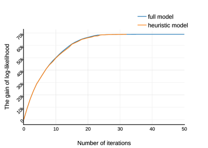
We first verify that the heuristic function $h(\alpha,\beta)$ proposed in Section 5 could discover the most informative patterns from $\mathcal{X}$ based on the current knowledge the model already knows. We refer the Maximum Entropy model inferred with entire pattern set $\mathcal{X}$ and all the individual attribute frequencies as full model, and the Maximum Entropy model selected by heuristic and BIC as heuristic model. Notice that in the heuristic model, individual attribute frequencies are also taken into account. In this experiment, we iteratively updated the model with the patterns in $\mathcal{X}$, and measured the log-likelihood in each iteration. However, using BIC to select the model may result different number of patterns incorporated over different synthetic datasets. Thus, we report the results over a single synthetic dataset here. For the full model, the pattern in $\mathcal{X}$ that maximized the log-likelihood in each iteration were selected and added to the model.

Table 2: Comparison of model preparation time ($t_{\mathit{pre}}$), model inference time ($t_{\mathit{infer}}$) and data sampling time ($t_{\mathit{sample}}$) between full model and heuristic model (in seconds).

	$t_{\mathit{pre}}$	$t_{\mathit{infer}}$	$t_{\mathit{sample}}$
full model	4438.785	27.266	1.678
heuristic model	17.981	8.950	0.461

Figure 3 illustrates the gain of the log-likelihood as the model incorporates more and more patterns in $\mathcal{X}$. As expected, the gain of the log-likelihood of the full model is larger in some iterations since it identifies the optimal pattern in each iteration with respect to the likelihood. We also observe that although not optimal, the log-likelihood of the heuristic model approximates that of the full model quite well, which demonstrates that the proposed heuristic successfully identifies the relatively informative patterns in each iteration. In the last few iterations, the gain of log-likelihood of the full model barely changes. This indicates that the patterns selected in these iterations are less informative or even redundant.

To assess the quality of the reconstruction, we aim to apply KL divergence measures. However, in practice, it is very difficult to compute the KL divergence between the entire Maximum Entropy distribution and data generating distribution for the categorical data due to the large categorical tuple space. As a trade off, we use the probabilities of patterns in pattern set $\mathcal{Y}$ to characterize the probability distributions for categorical data in both scenarios, and define the following approximate KL-divergence measure:

$$\mathit{\hat{KL}}(p^{*},p^{\prime})=\sum_{X\in\mathcal{Y}}\bigg{[}p^{*}(X)\log\frac{p^{*}(X)}{p^{\prime}(X)}+(1-p^{*}(X))\log\frac{1-p^{*}(X)}{1-p^{\prime}(X)}\bigg{]}~{}.$$

Here, $p^{*}$ and $p^{\prime}$ denote the Maximum Entropy distribution and data generating distribution respectively, and pattern set $\mathcal{Y}$ could be only categorical pattern set $\mathcal{X}$ or $\mathcal{X}\cup\mathcal{A}$ if individual attribute frequencies are considered. We also compute the $\mathit{\hat{KL}}(\tilde{p},p^{\prime})$ to compare the empirical probability distribution, say $\tilde{p}$, in the samples generated by the categorical Maximum Entropy model with the true data generating distribution. In this experiment, we computed $\mathit{\hat{KL}}(p^{*},p^{\prime})$ and $\mathit{\hat{KL}}(\tilde{p},p^{\prime})$ for both full model and heuristic model. For comparison purpose, we used independent attribute model $p_{\mathcal{A}}$ where each categorical attribute is independent of each other as the baseline model. For each of these models under consideration, 1000 categorical data samples were generated to compute empirical probability distribution $\tilde{p}$.

Figure 6: Comparison of two-attribute marginal distributions between true statistics in Virginia ACS summary data and samples generated by categorical Maximum Entropy model for categorical patterns {sex, age} (left), {sex, income} (middle), and {sex, marital status} (right). For pattern {sex, marital status}, the pattern values whose marital status is Others under 15 years old is not displayed here since for those individuals, their marital statuses are unavailable.

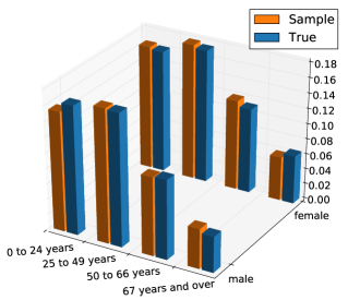
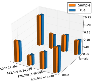
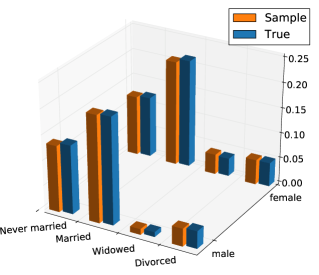
Table 1 compares these approximate KL-divergence measures. In Table 1, the small approximate KL-divergence values for full model and heuristic model indicate that the categorical Maximum Entropy distributions converge to the underlying data generation distribution. Moreover, the samples generated by these two models also successfully maintain the properties of the data generation distribution. This demonstrates that our model is capable of recovering the true categorical data distribution. When compared to the baseline model, our model outperforms several magnitudes in term of estimation accuracy.

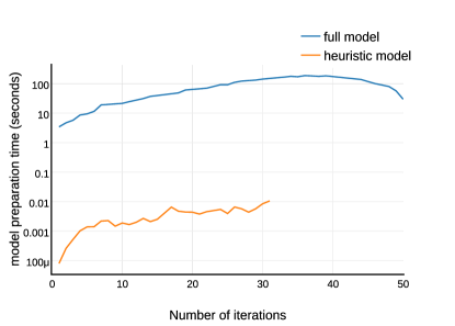
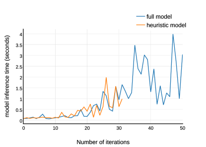
We also measure the time required to prepare the pattern set that serves as prior information of the model $t_{\mathit{pre}}$, the time to infer the Maximum Entropy model $t_{\mathit{infer}}$, and the time to sample a single categorical tuple from the model $t_{\mathit{sample}}$. Here, for the full model, $t_{\mathit{pre}}$ refers to the time required to arrange the pattern set $\mathcal{X}$ into the same order used in the iterative model update procedure in the first experiment where the categorical pattern that maximizes the log-likelihood is chosen in each iteration. Table 2 compares the runtime performance between the full model and the heuristic model, and Figure 5 and 5 show the $t_{\mathit{pre}}$ and $t_{\mathit{infer}}$ of every iteration in the iterative procedure used to verify the heuristic function $h(\alpha,\beta)$ in our first experiment. With the informative as well as simple model selected by the heuristic function $h(\alpha,\beta)$ and BIC, the heuristic model requires much less time to infer the Maximum Entropy distribution and sample categorical tuples from the model.

Figure 7: The gain of the negative log-likelihood of the model compared to the baseline model (model at iteration 0) over the Virginia ACS summary data. The data point marked with cross denotes the negative log-likelihood of the full model where all the categorical patterns in Virginia ACS summary data are considered.

6.3 Results on Real Data

To evaluate the performance of the proposed categorical Maximum Entropy model on the real data, we studied the problem of generating synthetic populations with US census data. Specifically, we use the 2012 American Community Survey (ACS) 1-year summary data [20], which contains aggregated statistics about age, sex, race, income, and many other features. Some of these features, e.g. sex and race, are perfect categorical attributes for the proposed Maximum Entropy model. While although some other features, e.g. age and income, are numerical, they are binned into several ranges based on their values, and treated here as categorical attributes.

Table 3: Top categorical patterns selected by heuristic model in Virginia ACS summary data.

patterns	number of possible values	number of selected values
{means of transportation to work, occupation}	49	34
{sex, income}	8	2
{sex, marital status}	10	2
{sex, age}	8	1

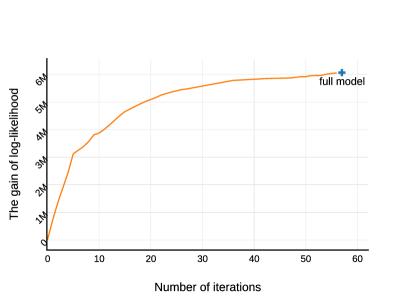
In our experiments, we chose the state of Virginia as our study case. Among all the features in the ACS summary data, we selected sex, age, race, income, occupation, marital status, means of transportation to work, education level, and health insurance coverage as the set of categorical attributes. We converted the corresponding aggregated statistics in ACS summary data into categorical patterns, and inferred the heuristic model over these patterns. Figure 7 describes the gain of the log-likelihood of the heuristic model, and the approximate KL-divergence measure between the inferred Maximum Entropy distribution and the empirical data distribution in Virginia ACS summary data is $0.0001975$. Table 3 also shows some most informative patterns selected by the proposed heuristic. Notice that in Figure 7, the last data point marked with cross indicates the gain of the log-likelihood of the full model where all the categorical patterns in the Virginia ACS summary data are taken into account.

We also generated a sample of $3,000$ synthetic individuals with the inferred heuristic model for Virginia, and calculated the marginal distributions for all individual attributes and some selected two-attribute categorical patterns. Notice that for attributes Marital status, Means of transportation to work, Occupation and Education level, the population considered in the ACS summary data is not the entire population of Virginia state. Thus, we add an additional value for these attributes, e.g. the value Others under 15 years old for the attribute Marital status, to denote the proportion of the entire population that are not taken into account in the ACS summary data. Fig. 6 show some of these marginal distributions and compares them with Virginia ACS summary data. We can see that the empirical distributions calculated from the synthetic individuals are very close to those in the Virginia ACS summary data. Such results demonstrate that our categorical Maximum Entropy model well maintains the statistical characteristics of the real world datasets, and is capable of generating synthetic data for real applications.

6.4 Application: Epidemic Simulation

Figure 8: The simulated weekly flu new infection counts compared to the estimated weekly new infection counts from Google Flu Trends. The simulation results are averaged across 10 independent runs.

In this section, we apply our proposed categorical Maximum Entropy model to generate synthetic population for the city of Portland OR in the United States, and use this model for an epidemiological simulation. We first take a publicly available synthetic contact network dataset of Portland [16], which contains both individual demographic and contact information of the residents in the city of Portland. The demographic information in this dataset contains gender, age and household income. We first group the values of age and household income into several ranges and change them into categorical features, similar to our ACS dataset analysis in Section 6.3. Then we compute the statistics, e.g. frequencies, of the single and pairwise demographic features, convert them into categorical patterns, and infer the categorical Maximum Entropy model over these patterns. The Portland dataset contains $1,575,861$ connected individuals, where each individual performs at least one activity with others. To generate our synthetic population for the Portland dataset, we draw $1,575,861$ samples from the inferred categorical Maximum Entropy model.

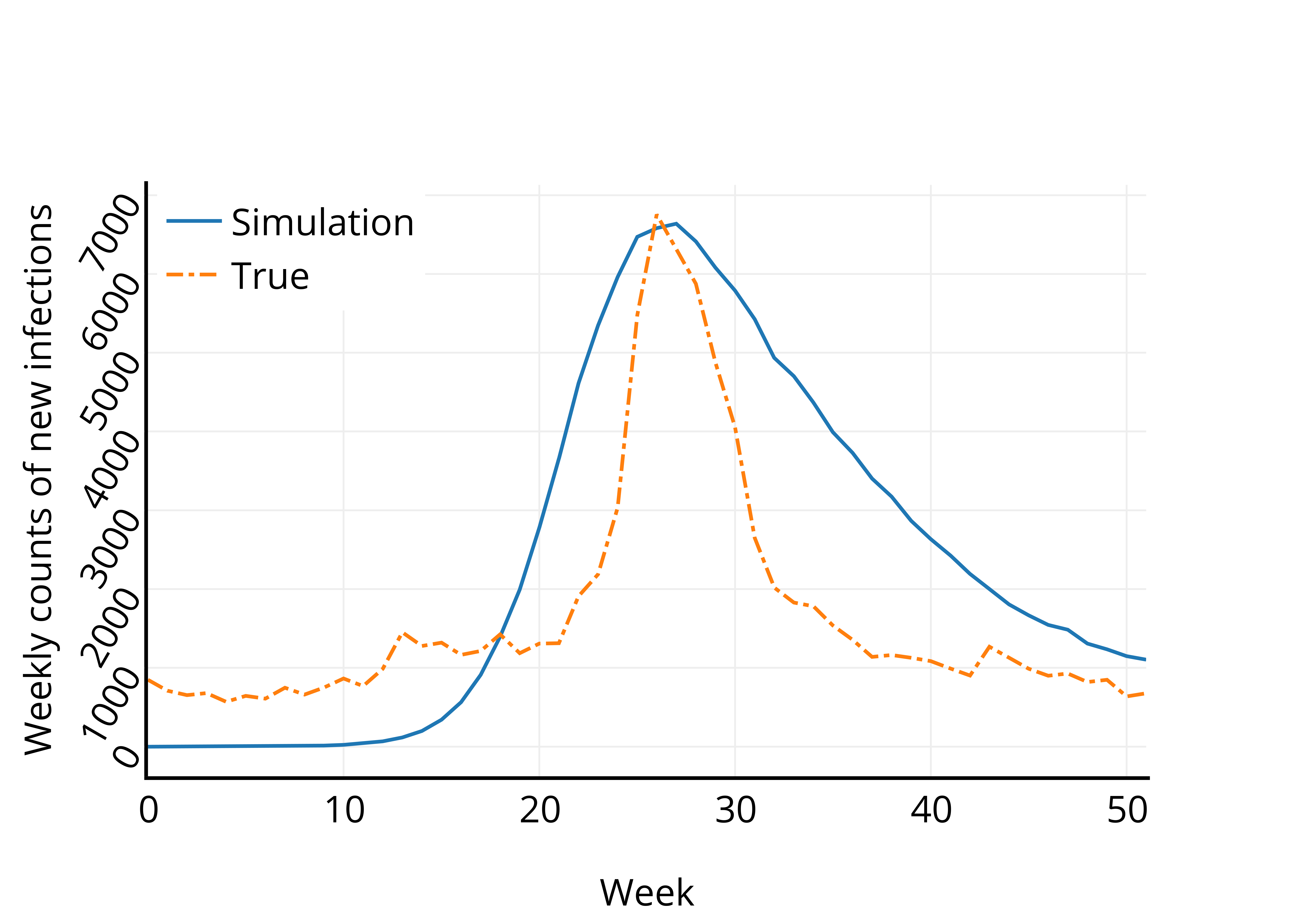
To construct the contact network for the synthetic population, we first match the generated synthetic individuals to the real ones involved in the contact activities described in the Portland dataset based on their demographical feature values. Then the contact network can be naturally created by connecting the synthetic individuals according to the contact activities they involves in. In this application, we choose to study the flu season in the city of Portland during the period from June 2013 to June 2014. We retrieve the estimated weekly counts of flu new infections for the city of Portland from Google Flu Trends [7], and apply the Susceptible-Infectious (SI) epidemic model over the contact network to fit the curve of weekly flu new infection counts. Figure 8 illustrates the fitted curve using the SI epidemic model. As the figure shows, the simulation results of the SI model over the synthetic population capture the trend and the peak of the weekly flu new infections in the city of Portland. These results demonstrate that the synthetic population generated by the categorical Maximum Entropy model is a useful model of population-level activity in cities.

7 Related Work

The problem of generating synthetic data that maintain the structures and dependencies in actual data has been studied by the researchers from various realms, ranging from network analysis to privacy preservation. The work in [2] studied and analyzed large synthetic social contact networks where the synthetic population was generated by applying iterative proportion fitting (IPF) techniques over census data. Variants of IPF, e.g. hierarchical IPF [13] and two-stage IPF [21], were also developed for generating synthetic population data for various research purposes such as land use and transportation microsimulation. Compared to the IPF-based approach, Ma and Srinivasan [11] proposed a fitness-based synthesis method to directly generate synthetic population, and Barthelemy and Toint [3] introduced a sample-free synthetic population generator by using the data at the most disaggregated level to define the joint distribution. Besides generating synthetic population with the combinational optimization based technique, Namazi-Rad et al. [14] also projected dynamics over the synthetic population using a dynamic micro-simulation model. The Network Dynamics and Simulation Science Laboratory at Virginia Tech released synthetic datasets of population in the city of Portland [16] and ad-hoc vehicular radio network in Washington D.C. [15], which are generated by the high-performance, agent-based simulation system Simfrastructure. Recently, Park et al. [17] proposed a non-parametric data synthesizing algorithm, particularly a perturbed Gibbs sampler, to generate large-scale privacy-safe synthetic health data. Instead of using patterns to characterize the data, a set of perturbed conditional probability distributions were estimated to represent the data distribution.

In the database community, there exists several research work that generates synthetic relational databases. For a survey, Gray et al. [8] discuss several database generation techniques that generate large scale synthetic datasets, and Bruno and Chaudhuri [4] proposed a Data Generation Language (DGL) that allows individual attribute distribution to be specified. In [9], the authors described a graph model directed database generation tool which could handle complex inter- and intra-table relationships in large database schemas.  Arasu et al. [1] proposed an efficient, linear programming based algorithm to generate synthetic relational databases that satisfy a given set of declarative constraints.

There is also extensive work related to the topic of query optimization that applies the Maximum Entropy principle in the database community. [10] and  [12] estimated the sizes of database queries by modeling complicated database statistics using Maximum Entropy probability distribution. Ré and Suciu [18] studied the problem of cardinality estimation using the Entropy Maximization technique, and proposed to use peak approximation to compute the approximate Maximum Entropy distribution. In [19], the authors described an algorithm called ISOMER which approximated the true data distribution by applying the Maximum Entropy principle over the information gained from database query feedback.

8 conclusion

In this paper, we propose a generative probabilistic model for the categorical data by employing Maximum Entropy principle. By introducing categorical tuple blocks and the corresponding partial order over them, we present an efficient model inference algorithm based on the well-known Iterative Scaling framework. Experiment results on both synthetic data and real US census data show that the proposed model well estimates the underlying categorical data distributions. The application to the problem of synthetic population generation demonstrates the potential of the proposed model to help the researchers in various areas.

References

- Arasu et al. [2011] Arvind Arasu, Raghav Kaushik, and Jian Li. Data generation using declarative constraints. In SIGMOD ’11, pages 685–696. ACM, 2011.
- Barrett et al. [2009] C.L. Barrett, R.J. Beckman, M. Khan, V. Kumar, M.V. Marathe, P.E. Stretz, T. Dutta, and B. Lewis. Generation and analysis of large synthetic social contact networks. In Simulation Conference (WSC), Proceedings of the 2009 Winter, pages 1003–1014, Dec 2009.
- Barthelemy and Toint [2013] Johan Barthelemy and Philippe L Toint. Synthetic population generation without a sample. Transportation Science, 47(2):266–279, 2013.
- Bruno and Chaudhuri [2005] Nicolas Bruno and Surajit Chaudhuri. Flexible database generators. In VLDB ’05, pages 1097–1107. VLDB Endowment, 2005.
- Csiszár [1975] Imre Csiszár. I-divergence geometry of probability distributions and minimization problems. Annals of Probability, 3(1):146–158, 1975.
- Darroch and Ratcliff [1972] J. N. Darroch and D. Ratcliff. Generalized iterative scaling for log-linear models. The Annals of Mathematical Statistics, 43(5):pp. 1470–1480, 1972. ISSN 00034851.
- [7] Google Inc. Data Source: Google Flu Trends. http://www.google.org/flutrends.
- Gray et al. [1994] Jim Gray, Prakash Sundaresan, Susanne Englert, Ken Baclawski, and Peter J. Weinberger. Quickly generating billion-record synthetic databases. In SIGMOD ’94, pages 243–252. ACM, 1994.
- Houkjær et al. [2006] Kenneth Houkjær, Kristian Torp, and Rico Wind. Simple and realistic data generation. In VLDB ’06, pages 1243–1246. VLDB Endowment, 2006.
- Kaushik et al. [2009] Raghav Kaushik, Christopher Ré, and Dan Suciu. General database statistics using entropy maximization. In DBPL ’09, pages 84–99. Springer-Verlag, 2009.
- Ma and Srinivasan [2015] Lu Ma and Sivaramakrishnan Srinivasan. Synthetic population generation with multilevel controls: A fitness-based synthesis approach and validations. Computer-Aided Civil and Infrastructure Engineering, 30(2):135–150, 2015.
- Markl et al. [2005] V. Markl, N. Megiddo, M. Kutsch, T. M. Tran, P. Haas, and U. Srivastava. Consistently estimating the selectivity of conjuncts of predicates. In VLDB ’05, pages 373–384. VLDB Endowment, 2005.
- Mueller and Axhausen [2011] Kirill Mueller and Kay W Axhausen. Hierarchical ipf: Generating a synthetic population for switzerland. In ERSA conference papers. European Regional Science Association, 2011.
- Namazi-Rad et al. [2014] Mohammad-Reza Namazi-Rad, Payam Mokhtarian, and Pascal Perez. Generating a dynamic synthetic population–using an age-structured two-sex model for household dynamics. PloS one, 9(4), 2014.
- [15] Network Dynamics and Simulation Science Laboratory. Synthetic data products for societal infrastructures and proto-populations: Data set 3.0. Technical report, Virginia Polytechnic Institute and State University. NDSSL-TR-07-010.
- [16] Network Dynamics and Simulation Science Laboratory. Synthetic data products for societal infrastructures and proto-populations: Data set 2.0. Technical report, Virginia Polytechnic Institute and State University. NDSSL-TR-07-003.
- Park et al. [2013] Y. Park, J. Ghosh, and M. Shankar. Perturbed gibbs samplers for generating large-scale privacy-safe synthetic health data. In Healthcare Informatics (ICHI), 2013 IEEE International Conference on, pages 493–498, Sept 2013.
- Ré and Suciu [2010] Christopher Ré and Dan Suciu. Understanding cardinality estimation using entropy maximization. In PODS ’10, pages 53–64. ACM, 2010.
- Srivastava et al. [2006] U. Srivastava, P. J. Haas, V. Markl, M. Kutsch, and T. M. Tran. ISOMER: Consistent histogram construction using query feedback. In ICDE ’06. IEEE Computer Society, 2006.
- United States Census Bureau [2012] United States Census Bureau. American community survey, 2012. URL http://www.census.gov/acs/www/.
- Zhu and Ferreira [2014] Yi Zhu and Joseph Ferreira. Synthetic population generation at disaggregated spatial scales for land use and transportation microsimulation. Transportation Research Record: Journal of the Transportation Research Board, 2429(1):168–177, 2014.