Effect of transverse anisotropy on inelastic tunneling spectroscopy of atomic-scale magnetic chains

Abstract

We theoretically investigate the effect of transverse magnetic anisotropy on spin-flip assisted tunneling through atomic spin chains. Using a phenomenological approach and first-order perturbation theory, we analytically calculate the inelastic tunneling current, differential conductance and atomic spin transition rates. We predict the appearance of additional steps in the differential conductance and a pronounced increase in the spin-flip transition rate which at low voltages scale quadratically with the ratio of the transverse anisotropy energy and the sum of the longitudinal anisotropy energy and the exchange energy. Our results provide intuitive qualitative insight in the role played by transverse anisotropy in inelastic tunneling spectroscopy of atomic chains and can be observed under realistic experimental conditions.

I Introduction

The development of small electronic storage devices has been going on for years and the possibility to store information in magnetic nanostructures is an active topic of research. A recent experiment has shown that information can in principle be stored in just a few antiferromagnetically aligned Fe atoms by using exchange coupling between atomic spins loth12 . This experiment involved imaging and manipulation of individual atomic spins by spin-polarized scanning tunneling microscopy (STM), a technique which over the last decade has developed into a powerful tool for studying spin dynamics of engineered atomic structures. In a series of seminal STM experiments inelastic tunneling spectroscopy (IETS) has been used to investigate spin excitation spectra of individual magnetic atoms hein04 , to probe the exchange interaction between spins in chains of Mn atoms and the orientation and strength of their magnetic anisotropy hirj06 ; hirj07 , and to study the effect of this anisotropy on Kondo screening of magnetic atoms otte08 . A few years later, experimental studies of tunneling-induced spin dynamics in atomically assembled magnetic structures were performed: In 2012 Loth et al. measured the voltage-induced switching rate between the two Néel ground states of an antiferromagnetically coupled chain of Fe atoms loth12 and recently spin waves (magnons) have been imaged in chains of ferromagnetically aligned atoms, including the demonstration of switching between the two oppositely aligned ground states and local tuning of spin state mixing by exchange coupling spin14 ; khat13 ; yan15 .
The tunnel-current-induced spin dynamics of single magnetic atoms and engineered atomic chains in these experiments can be well described by a spin Heisenberg Hamiltonian (see section II.1), which contains the magnetic anisotropy and exchange coupling between neighbouring atomic spins as phenomenological parameters. This model has been succesfully used to analyze, among others, the $I(V)$ characteristics of an electron interacting via exchange coupling with a magnetic atom hirj06 ; hirj07 ; otte08 ; fern09 , to explain step heights in inelastic conductance measurements of adsorbed Fe atoms lore09 ; soth10 , to provide a theoretical description based on rate equations of spin dynamics in one-dimensional chains of magnetic atoms delg10 , to analyze magnetic switching in terms of the underlying quantum processes in ferrromagnetic chains gauy13 and to calculate the electron-induced switching rate between Néel states in antiferromagnetic chains of Fe atoms gauy13PRL ; li15 ; tern15 .
In this paper we investigate the effect of single-spin transverse magnetic anisotropy on spin-flip assisted tunneling and spin transition rates in chains of magnetic atoms. Understanding the role played by magnetic anisotropy in tunnelling spectroscopy is of great importance both fundamentally and for being able to engineer magnetic properties of atomic chains and clusters on surfaces, as well as those of molecular magnets gatt06 ; burz15 . Compared with the longitudinal (easy-axis) magnetic anisotropy, the qualitative effect of transverse magnetic anisotropy on tunneling spectroscopy of magnetic chains has so far received little attention. In experiments involving antiferromagnetically coupled atoms transverse anisotropy has often been small (i.e. too small to be observable) to negligible, because the easy-axis anisotropy energy is much larger than the transverse exchange energy hirj06 ; hirj07 ; otte08 ; loth12 . However, such a uni-axial model does not always apply. Transverse anisotropy, together with the parity of the atomic spin, influences the degeneracy of the energy spectrum hirj07 ; delg12 ; jaco15 . Recent studies have demonstrated that the presence of non-zero transverse anisotropy modifies the switching frequency of few-atom magnets when atoms are directly adsorbed on the substrate khat13 . It has also been predicted that finite values of transverse anisotropy lead to the appearance of peaks in the differential conductance when using spin-polarized STM misi13 and a recent experiment has demonstrated that the strength of the magnetocrystalline anisotropy can be controllably enhanced or reduced by manipulating its local strain environment brya13 . In addition, ferromagnetically coupled atomic chains (nanomagnets) usually exhibit non-negligible values of transverse anisotropy spin14 ; khat13 ; yan15 . From an engineering point of view, transverse anisotropy could be used to tune dynamic properties such as spin switching in antiferromagnetic chains, since it breaks the degeneracy of the Néel ground states and transforms them into Néel-like states that contain a larger number of different spin configurations switching_vs_E . Recent experiments have investigated the three-dimensional distribution of the magnetic anisotropy of single Fe atoms and demonstrated the electronic tunability of the relative magnitude of longitudinal and transverse anisotropy yan15_2 . This provides further evidence for the potential importance of tunability of magnetic anisotropy for enhancing or weakening spin tunneling phenomena in magnetic adatoms and molecular magnets ober14 ; burz15 . Given all this, it is interesting and important to obtain direct and intuitive qualitative insight in the effect of transverse anisotropy on inelastic tunneling transport and STM-induced spin transition rates in chains of magnetic atoms. The aim of this paper is to provide a first step in this direction on a phenomenological level.
Using a perturbative approach and including the strength of the transverse anisotropy up to first order, we analytically calculate the inelastic current $I(V)$, differential conductance $dI/dV$ and corresponding IETS spectra $d^{2}I/dV^{2}$ for atomic chains with nearest-neighbour Ising exchange coupling. We also perform numerical simulations of spin transition rates of an antiferromagnetically coupled atomic spin chain. We find that finite transverse anisotropy introduces: 1) additional steps in the differential conductance $dI/dV$ and corresponding sharp peaks in $d^{2}I/dV^{2}$ and 2) a substantial increase of the spin transition rate between atomic levels. We show that both are due to transverse anisotropy-induced coupling between additional atomic spin levels and provide a qualitative explanation of the position and heights of the conductance steps and the dependence of the spin transition rates on the strength of the transverse anisotropy. Our perturbative approach is valid for single-spin transverse anisotropy strengths corresponding to typical experimental values.
The outline of the paper is as follows. In Sec. II A we discuss the phenomenological spin Hamiltonian and its energy spectrum and eigenfunctions with the transverse anisotropy energy included up to first-order perturbation theory. We then derive analytical expressions for the inelastic tunneling current $I(V)$, differential conductance $dI/dV$ and IETS spectra $d^{2}I/dV^{2}$ of an $N$-atomic spin chain (Sec. II B), and for the tunneling-induced transition rates (Sec. II C). Application of these results to chains of antiferromagnetically coupled atoms are presented and analyzed in Secs. III and IV. Sec. V contains conclusions and a discussion of open questions.

II Theory

II.1 Hamiltonian

In this section we first briefly discuss the spin Hamiltonian used to describe the atomic chain and then derive its eigenvalues and eigenfunctions up to first order in the strength of the transverse magnetic anisotropy.
The eigenenergies and spin eigenstates of a chain of $N$ magnetic atoms can be described by a phenomenological Heisenberg spin Hamiltonian, consisting of a single-spin part and nearest-neighbour exchange interaction hirj06 ; spin14 ; fern09 ; delg10 ; gatt06 :

$${\cal H}=\sum_{i=1}^{N}\hat{\cal H}_{i,S}+\sum_{i=1}^{N-1}J\,\hat{\bf S}_{i}\cdot\hat{\bf S}_{i+1}$$ (1)

with

$$\hat{\cal H}_{i,S}=D\hat{S}^{2}_{i,z}+E(\hat{S}^{2}_{i,x}-\hat{S}^{2}_{i,y})-g^{*}{\mu_{B}}{\bf B}\cdot\hat{\bf S}_{i}.$$ (2)

Here $D$ represents the single-spin longitudinal magnetocrystalline anisotropy, $E$ the transverse magnetic anisotropy, $g^{*}$ the Landé g-factor, $\mu_{B}$ the Bohr-magnetron, and ${\bf B}$ the external magnetic field. $J$ denotes the exchange energy between neighbouring atoms, which can be directionally dependent with different energies $J_{x}$, $J_{y}$ and $J_{z}$ for the three spin directions. In principle, $D$, $E$ and $J$ depend on the substrate and can vary from atom to atom. However, since experimentally the atom-to-atom variations are found to be small, see e.g. Refs. loth12 ; spin14 , these coefficients can to a good approximation be assumed to be uniform along the chain. $\hat{S}_{i,x}$, $\hat{S}_{i,y}$ and $\hat{S}_{i,z}$ are, respectively, the $x$-, $y$-, and $z$-components of the spin operator of the atom at site $i$ along the chain. Assuming ${\bf B}=B\hat{z}$, $E=0$ and exchange coupling between the $z$-components of the spin only (Ising coupling, see also the end of this section), the eigenvalues $E_{m_{1},...,m_{N}}$ of the Hamiltonian (1) are given by

$$E_{m_{1},...,m_{N}}=D\sum_{i=1}^{N}m_{i}^{2}+J\sum_{i=1}^{N-1}m_{i}m_{i+1}-E_{Z}\sum_{i=1}^{N}m_{i},$$ (3)

with corresponding eigenstates $|m_{1},..m_{N}\rangle^{(0)}$. Here $m_{i}$ denotes the quantum number labeling the angular momentum in the $z$-direction of the $i^{th}$ atom and $E_{Z}\equiv g^{*}\mu_{B}B$ represents the Zeeman energy. When adding the single-spin transverse anisotropy $E(\hat{S}^{2}_{i,x}-\hat{S}^{2}_{i,y})$ as a perturbation, the corresponding eigenfunctions $\psi_{m_{1},..,m_{N}}$ up to first order in $E$ are given by

$$\psi_{m_{1},\ldots,m_{N}}=|m_{1},..,m_{N}\rangle^{(0)}+|m_{1},..,m_{N}\rangle^{(1)},$$ (4)

with

$$|m_{1},...m_{N}\rangle^{(1)} = \frac{1}{2}E\,\sum_{i=1}^{N}$$

$$\left(\right.A_{m_{i-1},m_{i},m_{i+1}}|m_{1}..m_{i}\!+\!2..m_{N}\rangle^{(0)}\,-$$

$$\left.A_{m_{i-1},m_{i}-2,m_{i+1}}|m_{1}..m_{i}\!-\!2..m_{N}\rangle^{(0)}\right)$$

and

$$A_{m_{i-1},m_{i},m_{i+1}} \equiv$$

$$\left(36-12(m_{i}+1)^{2}\right. + \left.m_{i}(m_{i}+1)^{2}(m_{i}+2)+36\right)^{\frac{1}{2}}/$$

$$\left(-4D(m_{i}+1)\right. - \left.2J(m_{i-1}+m_{i+1})+2E_{Z}\right).$$ (6)

Here $A_{m_{j-1},m_{j},m_{j+1}}=0$ for $j<1$ or $m_{j-1},m_{j},m_{j+1}\notin[-2,..,2]$, $A_{m_{0},m_{1},m_{2}}\equiv A_{0,m_{1},m_{2}}$ and $A_{m_{N-1},m_{N},m_{N+1}}\equiv A_{m_{N-1},m_{N},0}$. Since the first-order correction of the eigenenergies (3) is zero, Eqns. (3) and (4) thus represent the eigenvalues and eigenfunctions of the Hamiltonian (1) (for ${\bf B}=B\hat{z}$ and Ising coupling) up to first order in $E$.
Figure 1 shows the energy spectrum (3) for a chain consisting of four Fe atoms (spin $s=2$) with antiferromagnetic coupling. The ground state of the chain consists of the two degenerate Néel states $|2,-2,2,-2\rangle^{(0)}$ and $|-2,2,-2,2\rangle^{(0)}$ with eigenenergy $16D-12J$.

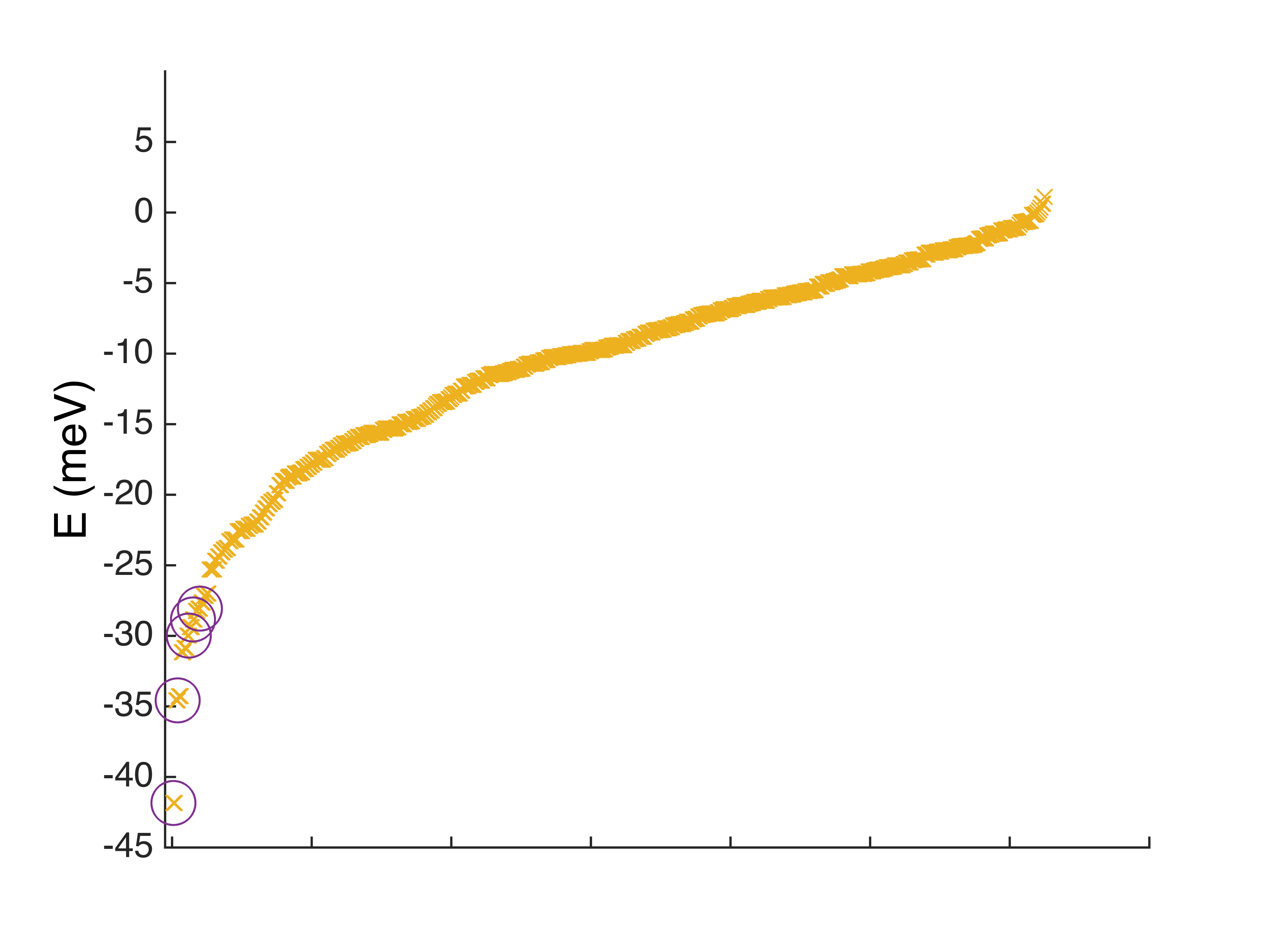
Figure 1: The energy spectrum $E\equiv E_{m_{1},..,m_{N}}$ [Eq. (3)] of an antiferromagnetically coupled chain consisting of four Fe atoms ($s=2$). Each cross represents an eigenstate, plotted in ascending order of energy. The circles mark the five eigenstates that contribute to the current and spin transition rates in Figs. 3-9. Parameters used are $D=-1.3$ meV, $J=1.7$  meV and $B=1$ T.

We end this section with a brief discussion of the assumption of Ising coupling in the Hamiltonian (1). This assumption is in general a good approximation for the description of atomic chains in which the longitudinal anisotropy is at least of the same order of magnitude as the exchange coupling, $|D/J|\gtrsim 1$, such as those studied in Refs. loth12 ; yan15 . When including the transverse anisotropy term in the Hamiltonian, which contains the off-diagonal spin operators $\hat{S}_{x}$ and $\hat{S}_{y}$, the question arises whether these non-Ising magnetic exchange terms pose additional requirements on the validity of the Ising approximation. We expect this approximation to be valid for atomic chains with predominantly longitudinal exchange coupling $|J_{x,y}/J_{z}|<<1$ (where the eigenstates are to a good approximation the eigenstates of the Ising model), and transverse anisotropy strengths $|J_{x,y}/E|\ll 1$ (so that $E$ is the dominant energy scale in the off-diagonal terms).

II.2 Current

A powerful technique to probe the spin dynamics of single magnetic atoms or small atomic chains deposited on a surface (typically a thin insulating layer on top of a metallic surface) is inelastic tunneling spectroscopy (IETS). In IETS, the spin of an electron tunneling from the tip of an STM interacts via exchange with the spin of an atom. When the energy provided by the bias voltage matches the energy of an atomic spin transition, the latter can occur and a new conduction channel opens jakl66 . For a chain consisting of $N$ magnetic atoms with spin $s=2$ (such as Fe or Mn) and the STM tip located above atom $j$ the inelastic current $I(V)$ in an IETS experiment is given by

$$I(V) = G_{S}\,\prod_{i=1}^{N}\,\left(\sum_{\stackrel{{\scriptstyle m_{i},m_{i}^{\prime}=-2}}{{\alpha=x,y,z;s=\pm}}}^{2}\!\right)\,P_{M}(V)\times$$ (7)

$$|\langle m_{1},..,m_{N}|S_{\alpha}^{(j)}|m_{1}^{\prime},..,m_{N}^{\prime}\rangle|^{2}\,F_{M,M^{\prime}\!,s}(V)$$

with

$$F_{M,M^{\prime},s}(V)\equiv\frac{eV-s\Delta_{M^{\prime}\!,M}}{1-e^{-s\beta(eV-s\Delta_{M^{\prime}\!,M})}}.$$ (8)

Eq. (7) is the $N$-atom generalization of the expression for the current given in Ref. fern09 . Here $|m_{1},..,m_{N}\rangle$ and $|m_{1}^{\prime},..,m_{N}^{\prime}\rangle$ denote the eigenstates of the Hamiltonian (1), $M$ represents the set of quantum numbers $(m_{1},..m_{N})$ corresponding to the eigenstate $|m_{1},..,m_{N}\rangle^{(0)}$ of the Hamiltonian (1) for ${\bf B}=B\hat{z}$, $E=0$ and Ising coupling, and $\Delta_{M^{\prime}\!,M}\equiv E_{M^{\prime}}-E_{M}$ with $E_{M}$ given by Eq. (3). $P_{M}(V)$ is the occupation of eigenstate $\psi_{m_{1},..,m_{N}}$ (see also the appendix), $\beta\equiv(k_{B}T)^{-1}$ and $S_{\alpha}^{(j)}$ with $\alpha=x,y,z$ is the local spin operator acting on atom $j$. The conductance quantum $G_{S}\sim\frac{2e^{2}}{h}\rho_{T}\rho_{S}T_{S}^{2}$ with $\rho_{T},\rho_{S}$ the density of states at the Fermi energy of the STM tip and surface electrodes and $T_{S}^{2}$ the tunneling probability between the local atomic spin and the transport electrons delg10 . Eq. (7) has been derived (for a single atomic spin) starting from a microscopic tunneling Hamiltonian that describes the exchange interaction between the spin of the tunneling electron and the atomic spin assuming short-range exchange interaction fern09 (alternative approaches that have been used to study spin-flip assisted transport in chains of magnetic atoms include nonequilibrium Green’s functions fran10 and generalized Anderson models delg11 ). The STM tip then only couples to the atom at site $j$ and the matrix element $|\langle m_{1},...,m_{N}|S_{\alpha}^{(j)}|m_{1}^{\prime},...m_{N}^{\prime}\rangle|^{2}$ describes the exchange spin interaction between the spin of the tunneling electron and this atomic spin: the generalization for coupling to several atoms is $|\langle m_{1},..,m_{N}|\vec{S}_{\alpha}|m_{1}^{\prime},..,m_{N}^{\prime}\rangle|^{2}$ with $\vec{S}_{\alpha}=\sum_{j}\eta(j)S_{\alpha}^{(j)}$ and $\eta(j)$ the tunnel probability through atom $j$, see Ref. fern09 . The function $F_{M^{\prime}\!,M,s}(V)$ on the right-hand side of Eq. (7) is the temperature-dependent activation energy for opening a new conduction channel: at energies where the applied bias voltage $eV$ matches the energy that is required for an atomic spin transition $\Delta_{M^{\prime}\!,M}$ a step-like increase in the differential conductance $dI/dV$ occurs. At these same voltages the second derivative of the current $d^{2}I/dV^{2}$ exhibits a peak (of approximately Gaussian shape). The area under these peaks corresponds to the relative transition intensity and is equal to the corresponding step height of the differential conductance yan15_2 . Analyzing $d^{2}I/dV^{2}$ data, commonly called IETS spectra, thus probes the transition probability between atomic spin levels. spin14 ; yan15

We now calculate the inelastic current (7) for a nonmagnetic STM tip by calculating the spin exchange matrix element for the eigenstates Eq. (4), i.e. using $|m_{1},..,m_{N}\rangle=\psi_{m1,..,m_{N}}$, and the occupation probabilities $P_{M}(V)$ for each eigenstate $|m_{1},..,m_{N}\rangle^{(0)}$. These populations $P_{M}(V)$ are obtained by solving the master equation delg10

$$\frac{dP_{M}(V)}{dt} = \sum_{M^{\prime}}P_{M^{\prime}}(V)W_{M^{\prime}\!,M}(V)\ -$$ (9)

$$P_{M}(V)\sum_{M^{\prime}}W_{M,M^{\prime}}(V),$$

with $W_{M,M^{\prime}}(V)$ the transition rate from atomic spin state $|m_{1},..,m_{N}\rangle^{(0)}$ to $|m_{1}^{\prime},..,m_{N}^{\prime}\rangle^{(0)}$. For small tunneling current, i.e. small tip (electrode)-atom coupling, the atomic chain is approximately in equilibrium and $P_{M}(V)$ can be approximated by the equilibrium population delg10 , which is given by the stationary solution of the master equation (9) (see the derivation in the appendix). Substitution of this solution and Eq. (4) into Eq. (7) yields the current $I(V)$:

$$I(V)=G_{S}\,(I^{(0)}(V)+I^{(1)}(V)).$$ (10)

Here

$$I^{(0)}(V) = \prod_{i=1}^{N}\sum_{\stackrel{{\scriptstyle m_{i}=-2}}{{s=\pm}}}^{2}P_{M}(V)\,\left\{(m_{j})^{2}\,F_{0,0,s}(V)\right.$$ (11)

$$+\frac{C_{m_{j}}}{2}\,F_{1,0,s}(V)$$

$$\left.+\,\frac{C_{m_{j}-1}}{2}\,F_{-1,0,s}(V)\right\}$$

$$I^{(1)}(V) = \frac{1}{8}\,E^{2}\,\prod_{i=1}^{N}\sum_{\stackrel{{\scriptstyle m_{i}=-2}}{{s=\pm}}}^{2}P_{M}(V)$$

$$\left\{8\,(A_{m_{j}}^{2}+A_{m_{j}-2}^{2})\,F_{0,0,s}(V)\right.$$

$$+ C_{m_{j}}\,B_{m_{j},2}^{2}\,F_{1,0,s}(V)$$

$$+ C_{m_{j}-1}\,B_{m_{j},0}^{2}\,F_{-1,0,s}(V)$$

$$+ A_{m_{j}-2}^{2}\left(C_{m_{j}-3}\,F_{-3,-2,s}(V)\right.$$

$$\left.\hskip 34.14322pt+\ C_{m_{j}-2}\,F_{-1,-2,s}(V)\right)$$

$$+ \left.A_{m_{j}}^{2}\left(C_{m_{j}+1}\,F_{1,2,s}(V)+C_{m_{j}+2}\,F_{3,2,s}(V)\right)\right\},$$

with

$$A_{m_{j}+n}^{2} \equiv A_{m_{j-1},m_{j}+n,m_{j+1}}^{2}$$ (13)

$$B_{m_{j},n}^{2} \equiv A_{m_{j-2},m_{j-1},m_{j}}^{2}+A_{m_{j-2},m_{j-1},m_{j}-1+n}^{2}+$$

$$A_{m_{j-2},m_{j-1}-2,m_{j}}^{2}+A_{m_{j-2},m_{j-1}-2,m_{j}-1+n}^{2}+$$

$$A_{m_{j-1},m_{j}-1+n,m_{j+1}}^{2}+A_{m_{j-1},m_{j}-3+n,m_{j+1}}^{2}+$$

$$A_{m_{j},m_{j+1},m_{j+2}}^{2}+A_{m_{j}-1+n,m_{j+1},m_{j+2}}^{2}+$$

$$A_{m_{j},m_{j+1}-2,m_{j+2}}^{2}+A_{m_{j}-1+n,m_{j+1}-2,m_{j+2}}^{2}$$

$$C_{m_{j}} \equiv 6-m_{j}(m_{j}+1)$$ (15)

$$F_{n_{1},n_{2},s} \equiv \frac{eV-s\Delta_{n_{2},n_{1}}}{1-e^{-s\beta(eV-s\Delta_{n_{2},n_{1}})}}$$ (16)

$$\Delta_{n_{2},n_{1}} \equiv E_{m_{1},..,m_{j}+n_{2},..,m_{N}}-E_{m_{1},..,m_{j}+n_{1},..m_{N}}$$ (17)

$$= (n_{2}-n_{1})\,\left((2m_{j}+n_{1}+n_{2})D\ +\right.$$

$$\left.(m_{j-1}+m_{j+1})J-E_{Z}\right).$$

$I^{(0)}(V)$ is the (zeroth-order) tunneling current in the absence of transverse anisotropy (for $E=0$) and $I^{(1)}(V)$ the additional contribution to this current for nonzero $E$ (up to first order in perturbation theory). $P_{M}(V)$ denotes the equilibrium population of state $\psi_{m_{1},..,m_{N}}$ (see also the appendix). The coefficient $A_{m_{j-1},m_{j},m_{j+1}}$ is given by Eq. (6). Fig. 2 schematically illustrates the eigenstates corresponding to the coefficients $A_{m_{j}+n}$ and $B_{m_{j},n}$ ((13) and (LABEL:eq:Bmj2)) for $m_{j}=m_{1}=2$.

Figure 2: Schematic illustration of the eigenstates contributing to the IETS current (10) for a four-atom chain in the ground state. Panel A: The unperturbed ground state $|2,-2,2,-2\rangle^{(0)}$. Panel B: The four unperturbed eigenstates contributing to the new ground state after including the transverse anisotropy energy to first order in perturbation theory. In each of these eigenstates $m_{i}$ differs by $-2$ (for $i=1,3$) or $+2$ (for $i=2,4$) from the unperturbed ground state in panel A (see also Eq. (4)). Panel C: The unperturbed eigenstates contributing to the IETS current if the STM tip is coupled to the first atom. In these eigenstates $m_{1}$ differs by $+1$ (upper row), $-1$ (middle row) or $0$ (lower row) compared to the states in panel B.

II.3 Transition Rates

In this section we derive expressions for the transition rates $W_{m_{1},..,m_{N}^{\prime}}\equiv W_{m_{1},..,m_{N},m_{1}^{\prime},..,m_{N}^{\prime}}$ between eigenstates $|m_{1},..,m_{N}\rangle$ and $|m_{1}^{\prime},..,m_{N}^{\prime}\rangle$ of the atomic spin chain up to first order in the transverse anisotropy energy $E$. These rates are also used to calculate the equilibrium occupation $P_{M}(V)$ of the energy levels, see the appendix. When an electron tunnels from the STM tip to the surface, or vice versa, and interacts with the atomic spin chain six types of spin transitions can occur delg10 , denoted by the rates $W_{m_{1},..m_{N}}^{S\to T}(V)$, $W_{m_{1},..,m_{N}^{\prime}}^{S\to S}$, $W_{m_{1},..,m_{N}^{\prime}}^{S\rightarrow T}(V)$, $W_{m_{1},..m_{N}}^{T\to S}(V)$, $W_{m_{1},..,m_{N}^{\prime}}^{T\to T}$, $W_{m_{1},..,m_{N}^{\prime}}^{T\rightarrow S}(V)$. Because of symmetry, $W_{m_{1},..,m_{N}^{\prime}}^{S\to S}=W_{m_{1},..,m_{N}^{\prime}}^{T\to T}$, and the pairs of rates $W_{m_{1},..m_{N}}^{S\to T}(V)$, $W_{m_{1},..m_{N}}^{T\to S}(V)$ and $W_{m_{1},..,m_{N}^{\prime}}^{S\rightarrow T}(V)$, $W_{m_{1},..,m_{N}^{\prime}}^{T\rightarrow S}(V)$ are identical upon reversal of the bias voltage, i.e. $W_{m_{1},..m_{N}}^{S\to T}(V)=W_{m_{1},..m_{N}}^{T\to S}(-V)$ and $W_{m_{1},..,m_{N}^{\prime}}^{S\rightarrow T}(V)=W_{m_{1},..,m_{N}^{\prime}}^{T\rightarrow S}(-V)$. Below we first discuss the physical process described by the rates $W_{m_{1},..m_{N}}^{S\to T}(V)$, $W_{m_{1},..,m_{N}^{\prime}}^{S\to S}$, and $W_{m_{1},..,m_{N}^{\prime}}^{S\rightarrow T}(V)$ (which also applies to resp. $W_{m_{1},..m_{N}}^{T\to S}(V)$, $W_{m_{1},..,m_{N}^{\prime}}^{T\to T}$, and $W_{m_{1},..,m_{N}^{\prime}}^{T\rightarrow S}(V)$ for reversed bias voltage) and then calculate these rates up to first order in $E$.
1. Elastic tunneling - $W_{m_{1},..m_{N}}^{S\to T}(V)$ denotes the rate for an electron tunneling from surface (S) to tip (T) without interacting with the atomic spin, i.e. without inducing a spin transition. This rate contributes to the elastic tunneling current.
2. Substrate-induced relaxation - $W_{m_{1},..,m_{N}^{\prime}}^{S\to S}$ corresponds to the simultaneous creation of an electron-hole pair in the surface electrode and a flip of the atomic spin from state $|m_{1},..,m_{N}\rangle$ to state $|m_{1}^{\prime},..,m_{N}^{\prime}\rangle$. This rate thus does not contribute to the current but does contribute to the equilibrium population $P_{M}$ at voltages that are sufficiently high for the atomic spin chain to be in an excited state. At low bias voltages $(W_{m_{1},..,m_{N}^{\prime}}^{S\to S})^{-1}$ is a measure for $T_{1}$, the atomic spin relaxation time delg10 .
3. Spin-flip assisted inelastic tunneling - $W_{m_{1},..,m_{N}^{\prime}}^{S\rightarrow T}(V)$ describes the transfer of an electron from surface to tip combined with a transition of the spin chain from spin state $|m_{1},..,m_{N}\rangle$ to state $|m_{1}^{\prime},..,m_{N}^{\prime}\rangle$. This process thus both contributes to the atomic spin dynamics and to the inelastic tunneling current. For an unpolarized STM tip the three rates can be calculated to lowest order in the electrode-chain coupling using Fermi’s golden rule. This results in:

$$W_{m_{1},..m_{N}}^{{\rm S}\,\to\,{\rm T}}(V) = \frac{4\pi}{\hbar}W_{1}\,\frac{eV}{1-e^{-\beta eV}}\times$$ (18)

$$\left|\sum_{\alpha=0}\langle m_{1},..m_{N}|S_{\alpha}^{(j)}|m_{1},..m_{N}\rangle\right|^{2}$$

$$= \frac{4\pi}{\hbar}W_{1}\frac{eV}{1-e^{-\beta eV}}$$

$$W_{m_{1},..m_{N}^{\prime}}^{{\rm S}\,\to\,{\rm S}} = \frac{4\pi}{\hbar}W_{2}\frac{\Delta_{M,M^{\prime}}}{1-e^{-\beta\Delta_{M,M^{\prime}}}}\ \times$$

$$\left|\sum_{\alpha=x,y}\langle m_{1},..m_{N}|S_{\alpha}^{(j)}|m_{1}^{\prime},..m_{N}^{\prime}\rangle\right|^{2}$$

$$W_{m_{1},..,m_{N}^{\prime}}^{{\rm S}\,\to\,{\rm T}}(V) = \frac{4\pi}{\hbar}W_{3}\,\frac{eV+\Delta_{M,M^{\prime}}}{1-e^{-\beta(eV+\Delta_{M,M^{\prime}})}}\,\times$$

$$\left|\sum_{\alpha=x,y,z}\langle m_{1},..m_{N}|S_{\alpha}^{(j)}|m_{1}^{\prime},..m_{N}^{\prime}\rangle\right|^{2},$$

with $W_{1}\equiv\rho_{S}\rho_{T}T_{0}^{2}$, $W_{2}\equiv\rho_{S}^{2}T_{J}^{2}$ and $W_{3}\equiv\rho_{S}\rho_{T}T_{J}^{2}$. $T_{0}$ and $T_{J}$ correspond to the direct (spin-independent) tunnel coupling and the tunneling-induced exchange coupling, respectively delg10 ; zhan13 . Calculating the total spin transition rates $W_{m_{1},..m_{N}}^{{\rm S}\,\to\,{\rm S}}$ $\equiv$ $\prod_{i=1}^{N}\,\left(\sum_{m_{i}^{\prime}=-2}^{2}\right)\,W_{m_{1},..,m_{N}^{\prime}}^{{\rm S}\,\to\,{\rm S}}$ and $W_{m_{1},..,m_{N}}^{{\rm S}\,\to\,{\rm T}}(V)$ $\equiv$ $\prod_{i=1}^{N}\,\left(\sum_{m_{i}^{\prime}=-2}^{2}\right)\,W_{m_{1},..,m_{N}^{\prime}}^{{\rm S}\,\to\,{\rm T}}(V)$ for the eigenstates $\psi_{m_{1},..m_{N}}$ [Eq. (4)] we obtain, up to first order in $E$ and for the STM tip coupled to atom $j$,

$$W_{m_{1}..m_{N}}^{{\rm S}\,\to\,{\rm S}} = \frac{2\pi}{\hbar}W_{2}\,\left\{C_{m_{j}}F_{1,0,+}(0)\,+C_{m_{j}-1}F_{-1,0,+}(0)\right.$$

$$+ \frac{E^{2}}{4}\,\left(C_{m_{j}}B_{m_{j},2}^{2}\,F_{1,0,+}(0)\right.$$

$$+ C_{m_{j}-1}B_{m_{j},0}^{2}\,F_{-1,0,+}(0)$$

$$+ A_{m_{j}-2}^{2}\,(C_{m_{j}-3}F_{-3,-2,+}(0)$$

$$+ C_{m_{j}-2}F_{-1,-2,+}(0))$$

$$+ \left.\left.A_{m_{j}}^{2}\,(C_{m_{j}+1}F_{1,2,+}(0)+C_{m_{j}+2}F_{3,2,+}(0))\right)\right\}$$

$$W_{m_{1}..m_{N}}^{{\rm S}\,\to\,{\rm T}}(V) = \frac{2\pi}{\hbar}W_{3}\,\left\{2m_{j}^{2}F_{0,0,+}(V)+\right.$$

$$C_{m_{j}}F_{1,0,+}(V)\,+\,C_{m_{j}-1}F_{-1,0,+}(V)+$$

$$\frac{E^{2}}{4}\,\left(8\,(A_{m_{j}}^{2}+A_{m_{j}-2}^{2})\,F_{0,0,+}(V)+\right.$$

$$C_{m_{j}}B_{m_{j},2}^{2}\,F_{1,0,+}(V)+$$

$$C_{m_{j}-1}B_{m_{j},0}^{2}\,F_{-1,0,+}(V)+$$

$$A_{m_{j}-2}^{2}\,(C_{m_{j}-3}F_{-3,-2,+}(V)+$$

$$C_{m_{j}-2}F_{-1,-2,+}(V))+$$

$$A_{m_{j}}^{2}\,(C_{m_{j}+1}F_{1,2,+}(V)+$$

$$\left.\left.C_{m_{j}+2}F_{3,2,+}(V))\right)\right\}.$$

Here $A_{m_{j}+n}^{2}$, $B_{m_{j},n}^{2}$, $C_{m_{j}}$ and $F_{n_{1},n_{2},s}$ are given by Eqns. (13)-(16).

III $I(V)$, $dI/dV$ and $d^{2}I/dV^{2}$

We now calculate the inelastic tunneling current [Eq. (10)], the corresponding differential conductance and the IETS spectra for the ground state of a chain consisting of $N$ atoms with antiferromagnetic coupling and analyze the effect of the transverse anisotropy energy $E$. For the (Néel-like) ground state $\psi_{-2,2,..,-2,2}$ [Eq. (4) with $m_{i}=-2$ for $i$ odd and $m_{i}=2$ for $i$ even] and the STM tip located above the first atom we obtain:

$$I_{\text{N\'{e}el}}(V)=G_{S}\,\left(I^{(0)}_{\text{N\'{e}el}}(V)+I^{(1)}_{\text{N\'{e}el}}(V)\right)$$ (23)

with

$$I^{(0)}_{\text{N\'{e}el}}(V) = 2\,\sum_{s=\pm}\left(2\,F_{0,0,s}(V)+F_{1,0,s}(V)\right)$$ (24)

$$I^{(1)}_{\text{N\'{e}el}}(V) = \frac{1}{4}\,E^{2}\,\sum_{s=\pm}\left\{4A_{0,-2,2}^{2}F_{0,0,s}(V)\right.$$ (25)

$$+\ 2\ B_{-2,2}^{2}F_{1,0,s}(V)$$

$$\left.+\,3\,A_{0,-2,2}^{2}(F_{1,2,s}(V)+F_{3,2,s}(V))\right\}.$$

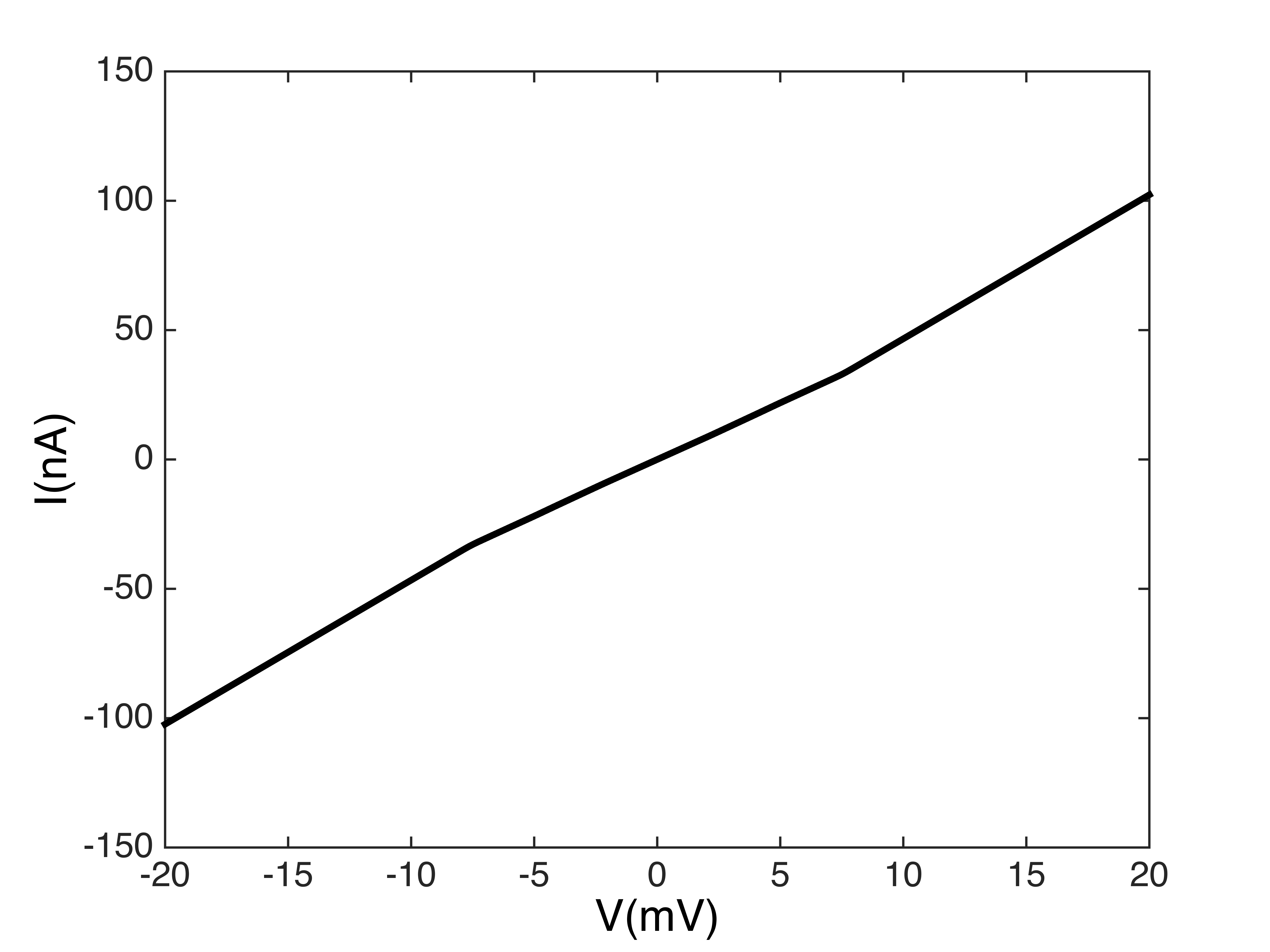
Figure 3: Inelastic tunneling current $I$ [Eq. (10)] normalized to the zero-bias conductance $G_{S}$ for an antiferromagnetic chain consisting of four atoms in the ground state $\psi_{2,-2,2,-2}$ with the STM tip coupled to the first atom. Parameters used are $D=-1.3$ meV, $E=0.3$ meV, $J=1.7$ meV, and $T=1$ K.

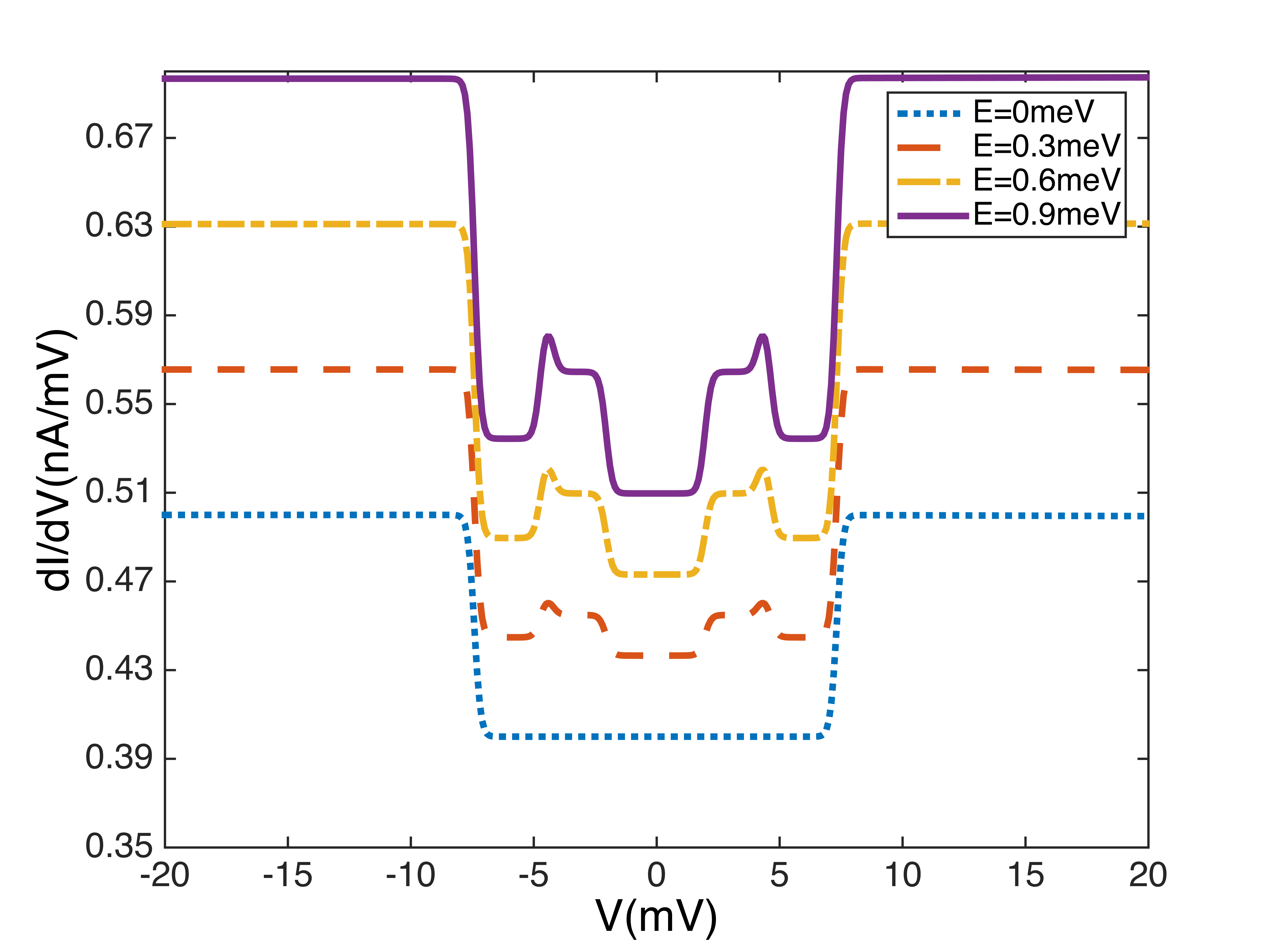
Figure 4: (color online) $dI/dV$ normalized to the zero-bias conductance $G_{S}$ for the chain in Fig. 3. Curves are shifted for clarity.

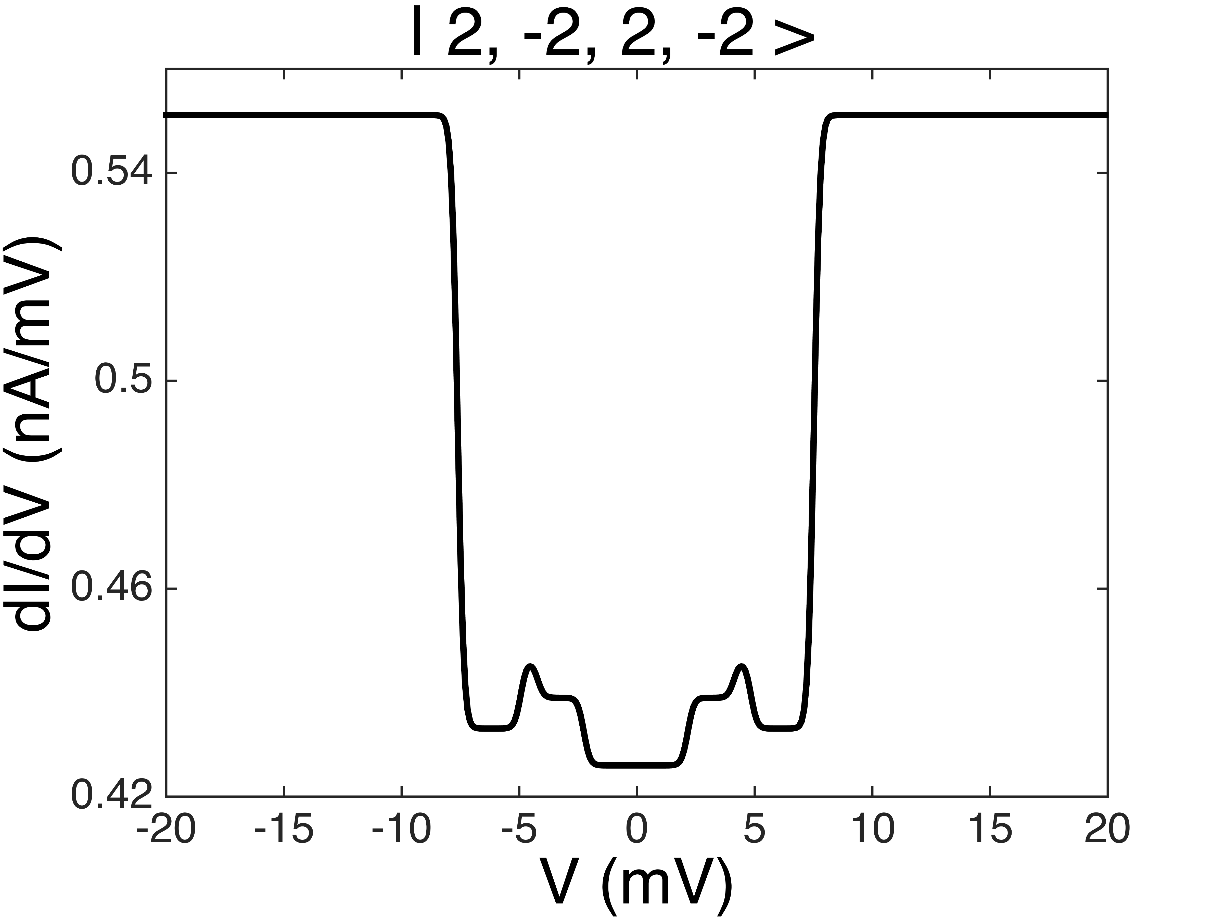
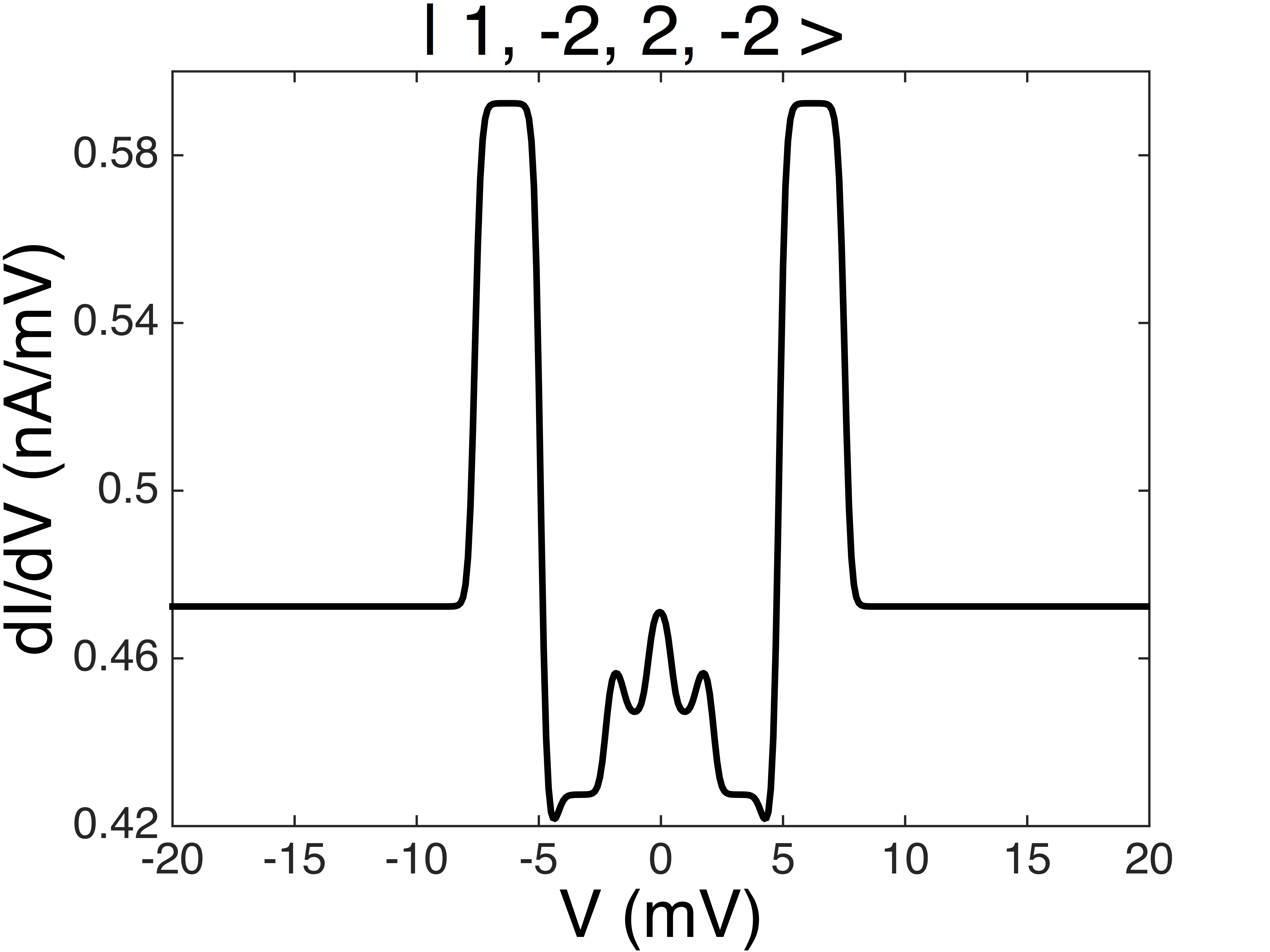
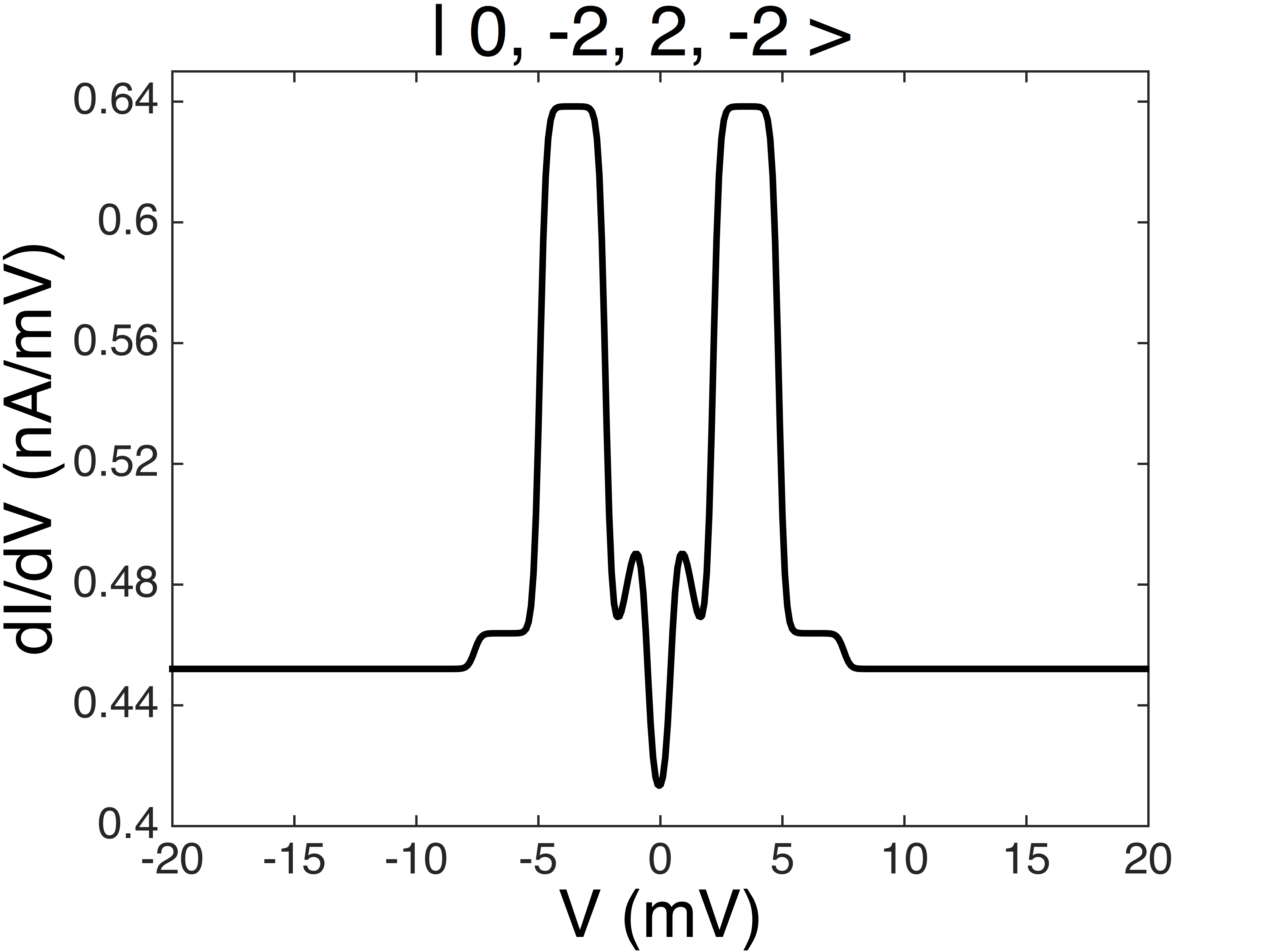
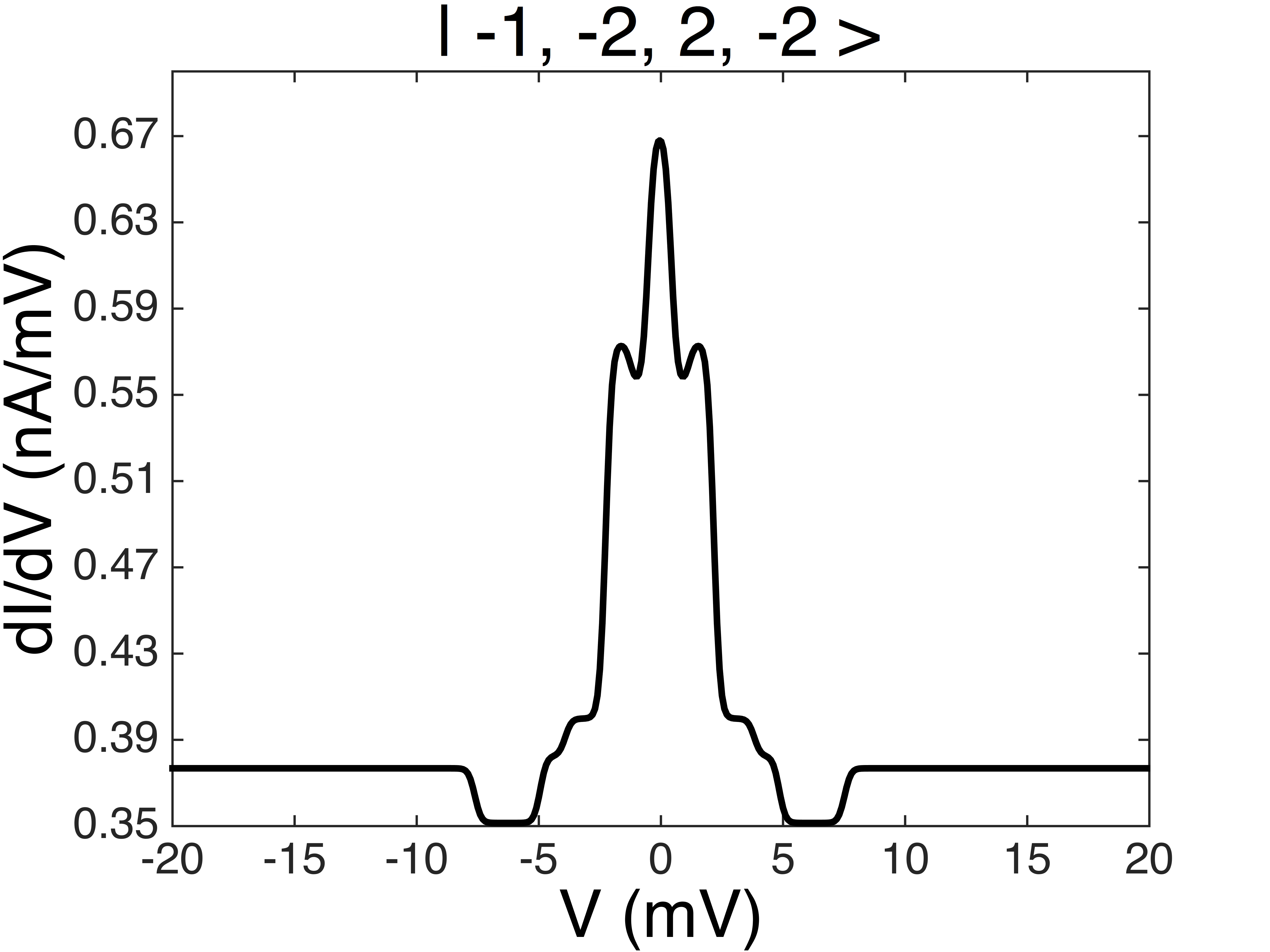
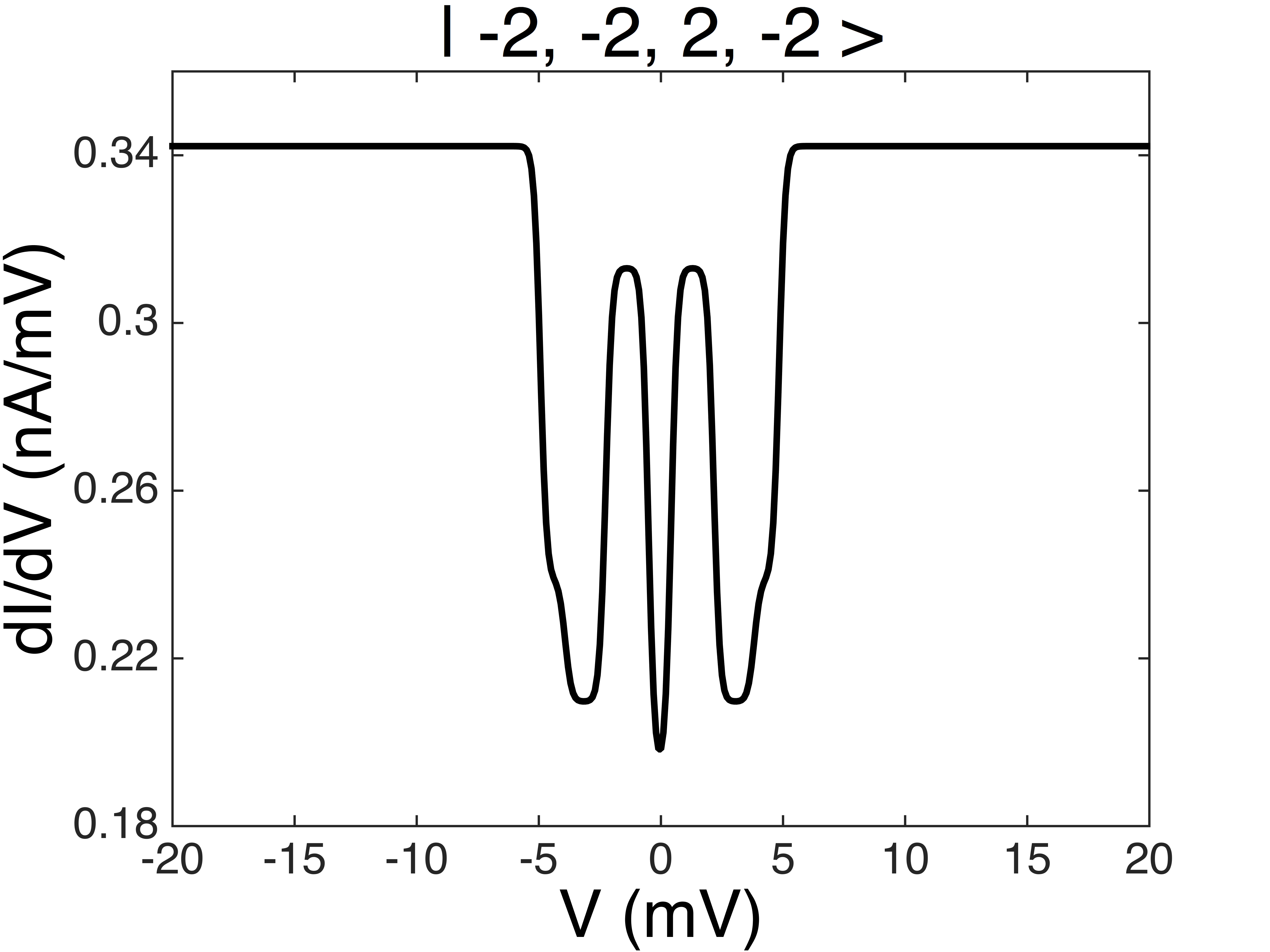
Figure 5: $dI/dV$ (normalized to the zero-bias conductance) of the five separate states $|m_{1},-2,2,-2\rangle$ with $m_{1}\in[2,..,-2]$ in the sums of Eqns. (11) and (LABEL:eq:currentE) for an antiferromagnetic chain in the ground state $\psi_{2,-2,2,-2}$ with the STM tip coupled to the first atom. Parameters used are the same as in Fig. 3.

The tunneling currents (24) and (25) depend on three energy gaps, corresponding to transitions between atomic spin levels with different values of $m_{1}$:

$$\Delta_{1} \equiv \Delta_{0,1}=3D-2J+E_{z}\ \ {\small(m_{1}\!=\!-2\!\rightarrow\!m_{1}\!=\!-1)}$$

$$\Delta_{2} \equiv \Delta_{2,1}=-D+2J-E_{z}\ \ (m_{1}\!=\!0\rightarrow m_{1}=-1)$$

$$\Delta_{3} \equiv \Delta_{2,3}=-D-2J+E_{z}\ \ (m_{1}=0\rightarrow m_{1}=1).$$

For the other Néel-like ground state $\psi_{2,-2,..,2,-2}$ the expressions (23)-(LABEL:eq:Neel2) are equivalent with only the signs of $m_{i}$, $i=1,..,N$, and the sign of $E_{z}$ reversed. Since $E_{z}\ll D,|J|$ the energy gaps (LABEL:eq:Neel2) are practically the same in both cases. In the derivation of Eq. (23) we have taken $P_{M}=1$ for the ground state and zero otherwise, since at low temperatures and voltages ($k_{B}T,eV\ll|\Delta_{1}|$) the equilibrium population of the excited states is negligible (see also Fig. 9 and discussion thereof in the text). The assumption that $P_{M}(V)$ is given by the equilibrium population may not be valid anymore at higher voltages when non-equilibrium effects start to play a role 2delg10 . Experimentally, $P_{|-2,2,..,-2,2\rangle^{(0)}}=1$ corresponds to using e.g. a half-metal tip.
Inspection of Eq. (23) using the requirement $I^{(1)}(V)\ll I^{(0)}(V)$ shows that our perturbative approach is valid for values of transverse anisotropy $E^{2}\ll J^{2},(D-J)^{2}$.
Fig. 3 shows the current $I(V)$ [Eq. (10), including all spin states and equilibrium populations $P_{M}$ for each state $|m_{1},..,m_{N}\rangle^{(0)}$] for typical experimental values khat13 ; spin14 ; yan15 of the transverse anisotropy strength $E$. As expected, the current increases linearly with $V$. It shows a kink (change of slope) at $eV\approx\pm|\Delta_{1}|\approx\pm 7.5$  meV, which corresponds to the energy gap between the ground state $|2,-2,..,2,-2\rangle^{(0)}$ and the first excited state $|1,-2,..,2,-2\rangle^{(0)}$ for $E=0$ of the atomic spin chain (the same argument applies for the other ground state $|-2,2,..,-2,2\rangle^{(0)}$). The increase in slope is to a very good approximation given by the coefficients of the corresponding activation energy terms $F_{1,0,s}(V)$ in Eqns. (24) and (25). The finite transverse anisotropy energy $E$ introduces additional kinks in the voltage region $-|\Delta_{1}|<eV<|\Delta_{1}|$. This can be seen more clearly in Fig. 4, which shows the differential conductance $dI/dV$ for the same chain for several values of the transverse anisotropy energy $E$. The large stepwise increase in $dI/dV$ at $eV\approx\pm|\Delta_{1}|\approx\pm 7.5$ meV in the figure corresponds to the kinks at these energies in Fig. 3. In addition, however, also steps in $dI/dV$ occur at voltages $eV\approx\pm|\Delta_{2}|$ and $eV\approx\pm|\Delta_{3}|$. These correspond to transitions between higher-lying excited states: The step in $dI/dV$ at $eV\approx|\Delta_{3}|\approx 2.3$  meV corresponds to the excitation from spin state $|0,-2,..,2,-2\rangle^{(0)}$ to state $|-\!1,-2,..,2,-2\rangle^{(0)}$. Then, around $eV\approx 4.9$  meV, a second step occurs, corresponding to the excitation from state $|1,-2,..,2,-2\rangle^{(0)}$ to $|0,-2,..,2,-2\rangle^{(0)}$. At this energy the excited state $|1,-2,..,2,-2\rangle^{(0)}$ has become somewhat populated allowing for this transition to occur step . At slightly higher voltage, however, a steplike decrease occurs, corresponding to decay from state $|0,-2,..,2,-2\rangle^{(0)}$ to state $|1,-2,..,2,-2\rangle^{(0)}$. Here the spin chain thus undergoes a transition from a higher-lying to a lower-lying state and an electron tunnels from drain (the STM tip) to source (the surface), thereby lowering the rate of increase of $I(V)$. Decays in differential conductance have been experimentally observed in STM measurements of magnetic atoms (see e.g. Ref. otte08 ; loth10 ) and were explained in terms of the non-equilibrium occupation of different spin levels, i.e. competition between depletion of one spin level in favour of another multiplied by the intensity (determined by the matrix elements) of the corresponding transitions.
Fig. 5 provides a more detailed illustration of the competition between these two processes. This figure shows each of the five terms $m_{1}$ $\in$ $[2,...,-2]$ that contribute to $dI/dV$ in Fig. 4 separately (the current (10) is the sum of these five terms weighed by the equilibrium population $P_{M}$ for each state). When inspecting the figure, we see that in the panels corresponding to $m_{1}=1$ and $m_{1}=0$ a sharp increase of $dI/dV$ occurs at, resp., energies $eV\approx|\Delta_{2}|\approx 4.9$ meV and $eV\approx|\Delta_{3}|\approx 2.3$ meV. Here the chain undergoes a transition to the next higher-lying state (from $m_{1}=1$ to $m_{1}=0$ and from $m_{1}=0$ to $m_{1}=-1$, resp.) In the same two panels the differential conductance subsequently decreases at voltages $eV\approx|\Delta_{1}|\approx 7.5$ meV and $eV\approx|\Delta_{2}|\approx 4.9$ meV, when the spin chain decays to the next lower-lying state. Similar analysis applies for the steps in the other panels.
Note that the position at which steps in $dI/dV$ occur does not depend on the strength of the transverse anisotropy, since the energy gaps $\Delta_{1}-\Delta_{3}$ in Eq. (LABEL:eq:Neel2) are independent of $E$ (up to first order in $E$). The onset of these in-gap steps is affected when $D$ is not constant along the chain, but varies from atom to atom (as e.g. in the experiment described in Ref. yan15 ). Within the parameter range of $D$, $J$ and $E$ that we consider (described in Sec. V) atom-to-atom variations in $D$ lead to small variations in the onset and the heights of the steps. The latter step heights at $eV=\Delta_{n_{1},n_{2}}$ scale with $E^{2}$ and are to a good approximation given by the (sum of the) prefactors $F_{n_{1},n_{2},s}$ in Eq. (23); for example, the step height at $eV\approx\pm|\Delta_{3}|$ is given by $(3/4)E^{2}A_{0,-2,2}^{2}\approx E^{2}/(D-J)^{2}$ (for small Zeeman energy). This step height is a direct measure for the spin excitation transition intensity. Finally, in the limit $|eV|\gg|\Delta_{1}|$, the differential conductance saturates at

$$\frac{dI_{\text{N\'{e}el}}}{dV} \stackrel{{\scriptstyle|eV|\gg|\Delta_{1}|}}{{\rightarrow}} 6eG_{S}\left(1+\frac{E^{2}}{12}\,(5A_{0,-2,2}^{2}+2B_{-2,2}^{2})\right)$$

$$\approx 6eG_{S}\left(1+\frac{E^{2}}{8}\,\left(\frac{5}{(D-J)^{2}}+\frac{3}{J^{2}}\right)\right).$$

The second line in Eq. (LABEL:eq:limitingvalue) is valid when the Zeeman energy is small, $|E_{z}|\ll|J|,|D-J|$. Fig. 6 shows the IETS spectra $d^{2}I/dV^{2}$ corresponding to the differential conductance $dI/dV$ in Fig. 4. The additional peaks and valleys induced by the finite transverse anisotropy strength in the voltage region between -7.5 meV and 7.5 meV can clearly be seen.
Finally, from an experimental point of view Eqns. (LABEL:eq:Neel2) can be used to extract the values of $D$ and $J$ from $dI/dV$ data. The height of measured in-gap steps can subsequently be used to obtain the strength of transverse anisotropy $E$.

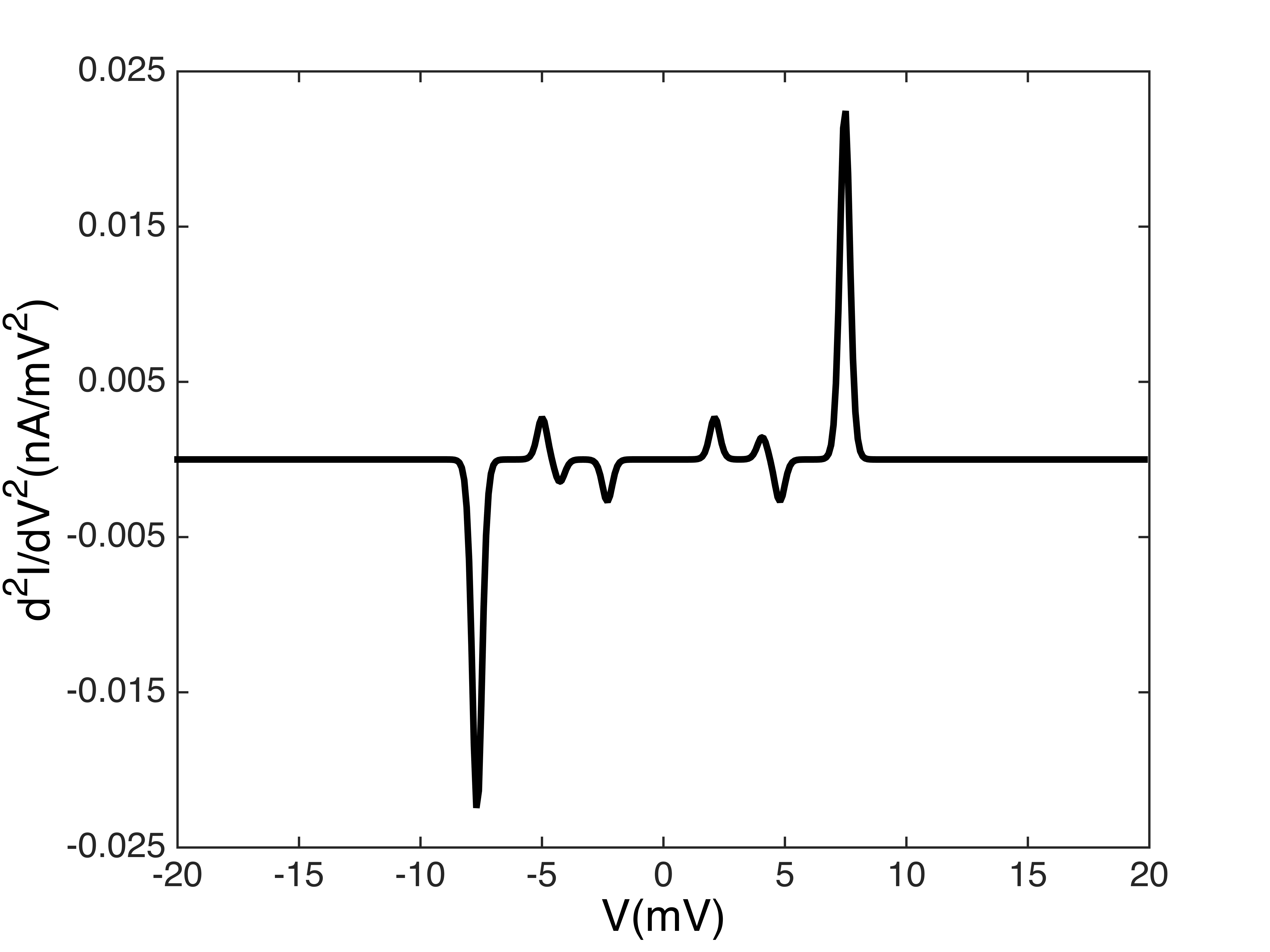
Figure 6: $d^{2}I/dV^{2}$ spectra corresponding to the differential conductance $dI/dV$ shown in Fig. 4 for $E=0.3$  meV.

IV Transition Rates

In this section we analyze the transition rates $W_{m_{1},..,m_{N}}^{S\to S}$ and $W_{m_{1},..,m_{N}}^{S\to T}(V)$ [Eqns. (LABEL:eq:matrixelement6) and (LABEL:eq:matrixelement5)] for the ground state $\psi_{-2,2,..,-2,2}$ of an antiferromagnetic $N$-atomic spin chain. By evaluating the matrix element in Eqns. (LABEL:eq:matrixelement6) and (LABEL:eq:matrixelement5) this results in, for the STM tip coupled to the first atom,

$$W_{\text{N\'{e}el}}^{{\rm S}\,\to\,{\rm S}} = \frac{8\pi}{\hbar}W_{2}\,\left\{F_{1,0,+}(0)+\frac{E^{2}}{8}\left(2B_{-2,2}^{2}\,F_{1,0,+}(0)\right.\right.$$ (28)

$$\left.\left.+\,3A_{0,-2,2}^{2}(F_{1,2,+}(0)+F_{3,2,+}(0)\right)\right\}$$

and

$$W_{\text{N\'{e}el}}^{{\rm S}\,\to\,{\rm T}}(V) = \frac{8\pi}{\hbar}W_{3}\,\left\{2\,F_{0,0,+}(V)\ +F_{1,0,+}(V)\,+\right.$$

$$\frac{E^{2}}{8}\left(4A_{0,-2,2}^{2}F_{0,0,+}(V)\right.$$

$$\ +\ 2B_{-2,2}^{2}\,F_{1,0,+}(V)$$

$$\left.\left.+\ 3A_{0,-2,2}^{2}(F_{1,2,+}(V)+F_{3,2,+}(V))\right)\right\},$$

with $\Delta_{1}$, $\Delta_{2}$ and $\Delta_{3}$ given by Eqns. (LABEL:eq:Neel2).

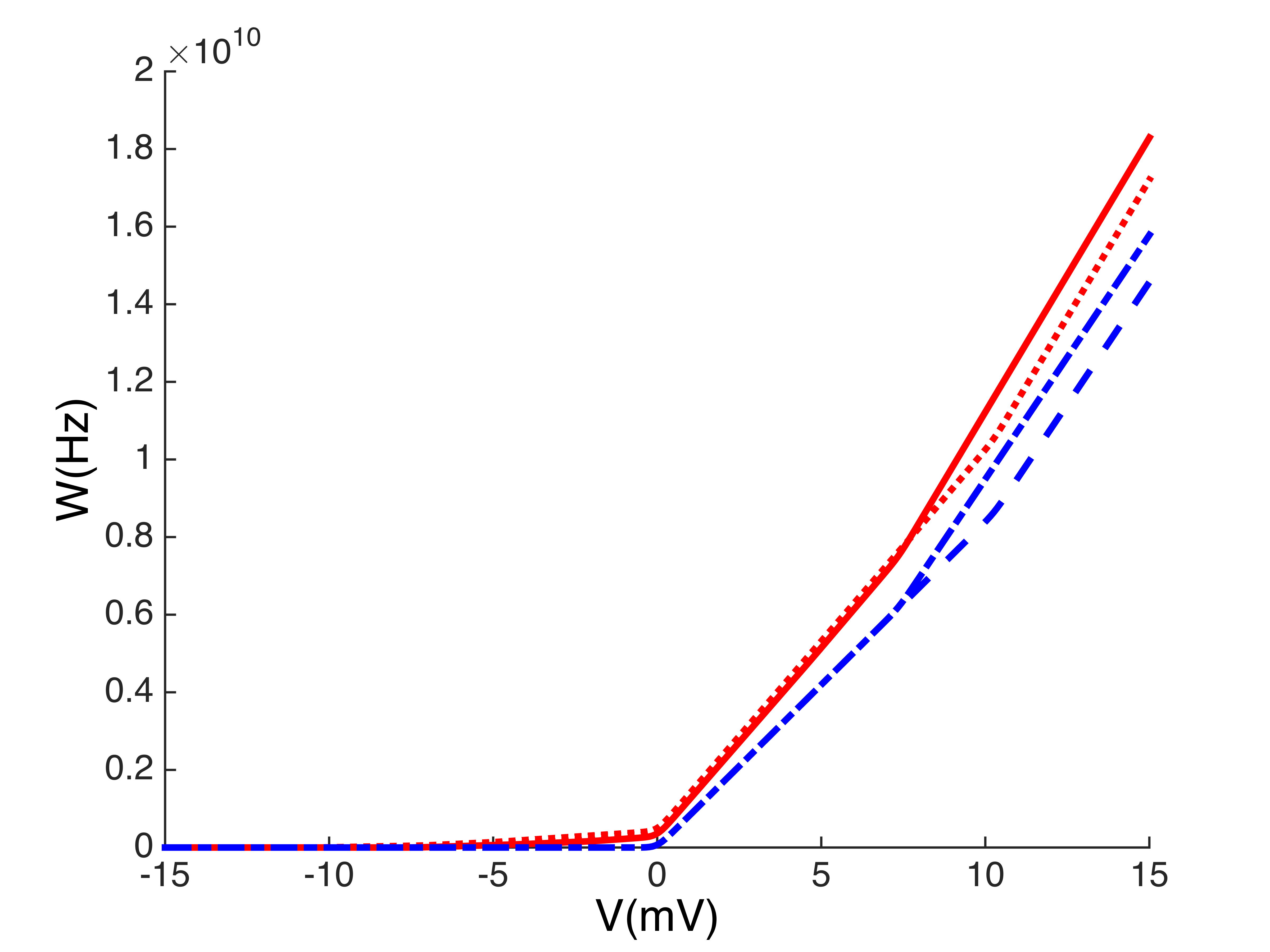
Figure 7: (Color online) The spin transition rate $W\equiv W_{\text{N\'{e}el}}^{S\rightarrow T}(V)$ [Eq. (LABEL:eq:matrixelement5)] for an antiferromagnetic atomic chain in the ground state with the STM tip coupled to the first atom and $E=0.3$ meV or $E=0.6$ meV (blue dot-dashed line and red solid line, respectively) and with the tip coupled to the second atom and $E=0.3$ meV or $E=0.6$ meV (blue dashed line and red dotted line, respectively). Other parameters used are $D=-1.3$  meV, $J=1.7$  meV, $B=1$  T and $W_{3}=1.1\times 10^{-5}$ (the latter value is taken from the experiment in Ref. spin14 ).

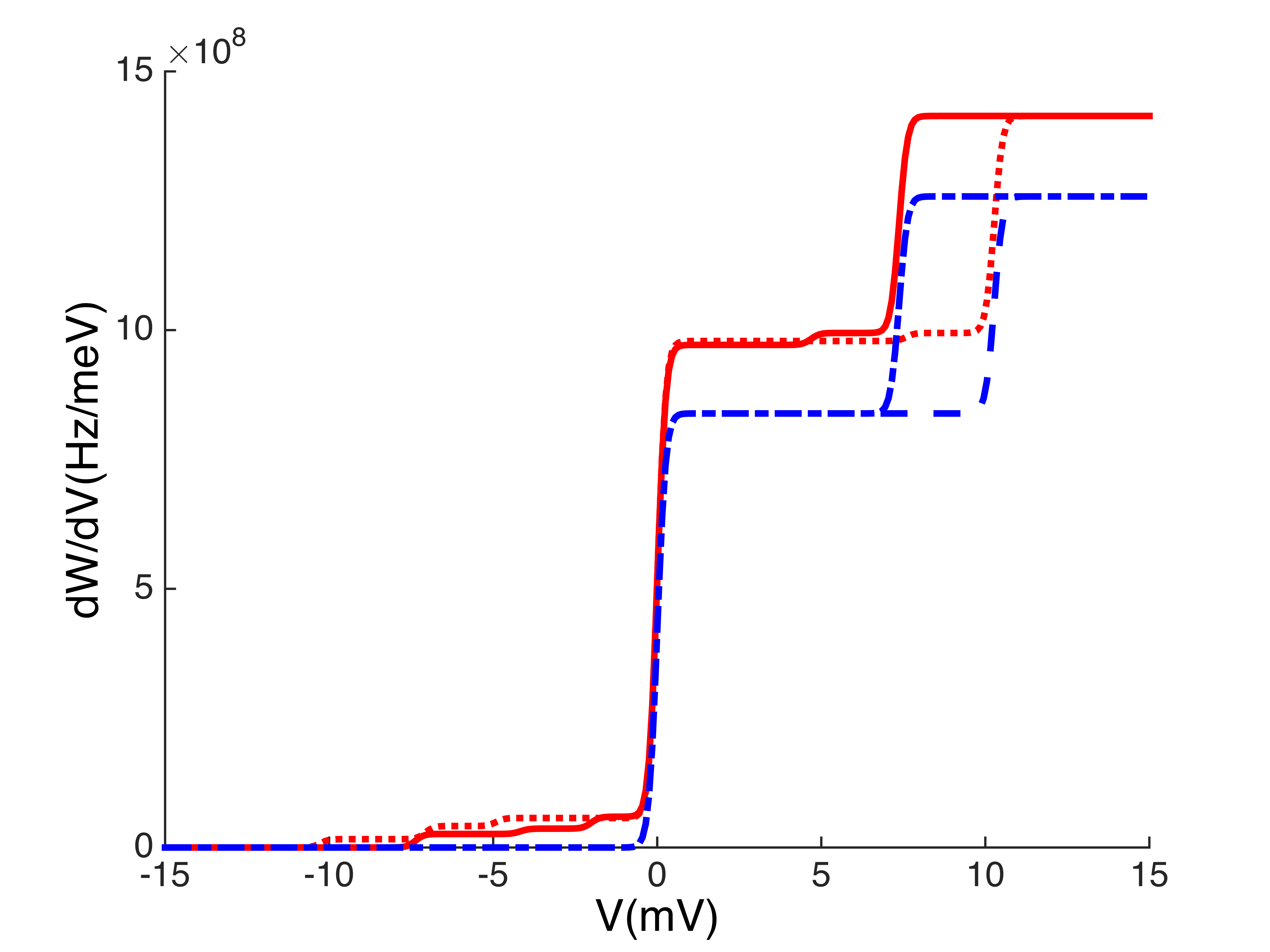
Figure 8: (Color online) First derivative of the transition rates $W_{\text{N\'{e}el}}^{S\rightarrow T}(V)$ in Fig. 8.

Fig. 8 shows $W^{S\to T}_{\text{N\'{e}el}}(V)$ for the STM tip coupled to either the first or the second atom along the chain. As expected, when the tip interacts with the first atom, $W^{S\to T}_{\text{N\'{e}el}}(V)$ exhibits a clearly visible kink (change of slope) at the same voltage $eV=|\Delta_{1}|\sim 7.5$ meV as the inelastic current in Fig. 3, which corresponds to the energy gap between the ground state and the first excited state of the chain (for the tip coupled to the second atom this gap is larger, given by $3D-4J-E_{Z}\approx 10.5$  meV). In addition, the finite transverse anisotropy energy also here induces additional kinks at $eV=|\Delta_{2}|$ and $eV=|\Delta_{3}|$. The positions of these kinks can be seen more clearly in the graph of the derivative $dW^{S\to T}_{\text{N\'{e}el}}/dV$ in Fig. 8. The onset of $W^{S\to T}_{\text{N\'{e}el}}$ at $V=0$ meV is due to thermally activated elastic tunneling.
Fig. 8 also shows that finite transverse anisotropy energy increases the spin transition rates $W^{S\to T}_{\text{N\'{e}el}}(V)$ for any value of the voltage $V$. From Eq. (LABEL:eq:Neel3) and the tip coupled to the first atom we find that this relative increase scales as $E^{2}/(D-J)^{2}$ for energies $eV\ll|\Delta_{1}|$ and as $\frac{E^{2}}{8}\,\left(\frac{5}{(D-J)^{2}}+\frac{3}{J^{2}}\right)$ for energies $eV\gtrsim|\Delta_{1}|$. For the voltage-independent relaxation rate $W^{S\to S}_{\text{N\'{e}el}}$ (not shown in Fig. 8) we obtain from Eq. (28) for $|E_{z}|\ll|D-J|,|J|$

$$W^{S\to S}_{\text{N\'{e}el}}\approx\frac{8\pi}{\hbar}W_{2}\left|\Delta_{1}\right|\left(1+\frac{9}{16}\,\frac{E^{2}}{J^{2}}\right).$$

Since $T_{1}\sim 1/W^{S\to S}_{\text{N\'{e}el}}$ at low bias voltages, the presence of finite transverse anisotropy energy thus leads to a decrease of the spin relaxation time which scales as $E^{2}/J^{2}$.

V Summary and Conclusions

We have presented a perturbative theory for the effect of single-spin transverse magnetic anisotropy on tunneling-induced spin transitions in atomic chains with Ising exchange coupling. We qualitatively predict the dependence of the inelastic tunneling current $I$ and the transition rates between atomic spin levels on the transverse anisotropy energy $E$ and show that the presence of finite values of $E$ leads to additional steps in the differential conductance $dI/dV$ and to higher spin transition rates. For an antiferromagnetically coupled chain in the Néel ground state both the heights of the additional steps and the increase in spin transition rates at low bias voltage scale as $E^{2}/(D-J)^{2}$, while the latter crosses over to $E^{2}/J^{2}$ scaling for higher voltages $eV\gtrsim|\Delta_{1}|$.

Our model is relevant for materials in which the easy-axis exchange interaction dominates over the transverse exchange interaction (justifying the use of the Ising Hamiltonian), measurements at low current with a non-magnetic STM tip and for values of transverse anisotropy $E^{2}/J^{2},E^{2}/(D-J)^{2}\ll 1$. The latter requirement is in agreement with typical values of $E$, $D$ and $J$ measured in chains of, for example, Fe or Mn atoms loth12 ; hein04 ; hirj06 ; hirj07 ; otte08 ; spin14 ; khat13 ; yan15 , where $D$ varies between -2.1 and -1.3 meV, J is in the range 1.15-1.6 meV, and E is 0.3-0.31 meV. We therefore expect our results to be applicable for antiferromagnetically coupled chains consisting of these and similar magnetic atoms with little-to-none local distortion between atoms and deposited on a flat symmetric substrate, so that spin-orbit interaction (and thereby induced Dzyaloshinskii-Moriya interaction) is weak and can be neglected.

Our model could be used to extract the values of $D$ and $J$ from the onset of the in-gap steps in measurements of $dI/dV$, since these threshold voltages are directly related to energy gaps between spin levels, see Eq. (LABEL:eq:Neel2). The height of these in-gap steps can subsequently be used to extract the value of $E$. In fact, with a note of caution, in-gap features in $dI/dV$ may actually be present in Fig. 2(c) of Ref. yan15 . Using the parameters from this experiment ($D$=-2.1 meV, $J$=1.15 meV, $E$=0.31 meV and $B$=2 T) in our model there would be additional steps in dI/dV at bias voltages $V$=1.6 mV and $V$=4 mV with heights on the order of 0.01-0.02 $\mu S$. Looking at the two uppermost curves in Fig. 2(c) in Ref. yan15 a small steplike feature does seem to be present at each of these voltages. These possible hints at in-gap $dI/dV$ features of course need to be checked - whether they exist could e.g. be verified by data for larger values of transverse anisotropy strength, which we believe would be very interested to investigate.

Finally, interesting questions for future research are to study the effect of transverse anisotropy on non-equilibrium spin dynamics in chains of magnetic atoms, on dynamic spin phenomena such as the formation of e.g. magnons, spinons and domain walls, and on switching of Néel states in antiferromagnetically coupled chains. We acknowledge valuable discussions with F. Delgado and A.F. Otte. This work is part of the research programme of the Foundation for Fundamental Research on Matter (FOM), which is part of the Netherlands Organisation for Scientific Research (NWO).

Appendix A Equilibrium populations ${\bf P_{M}}(V)$

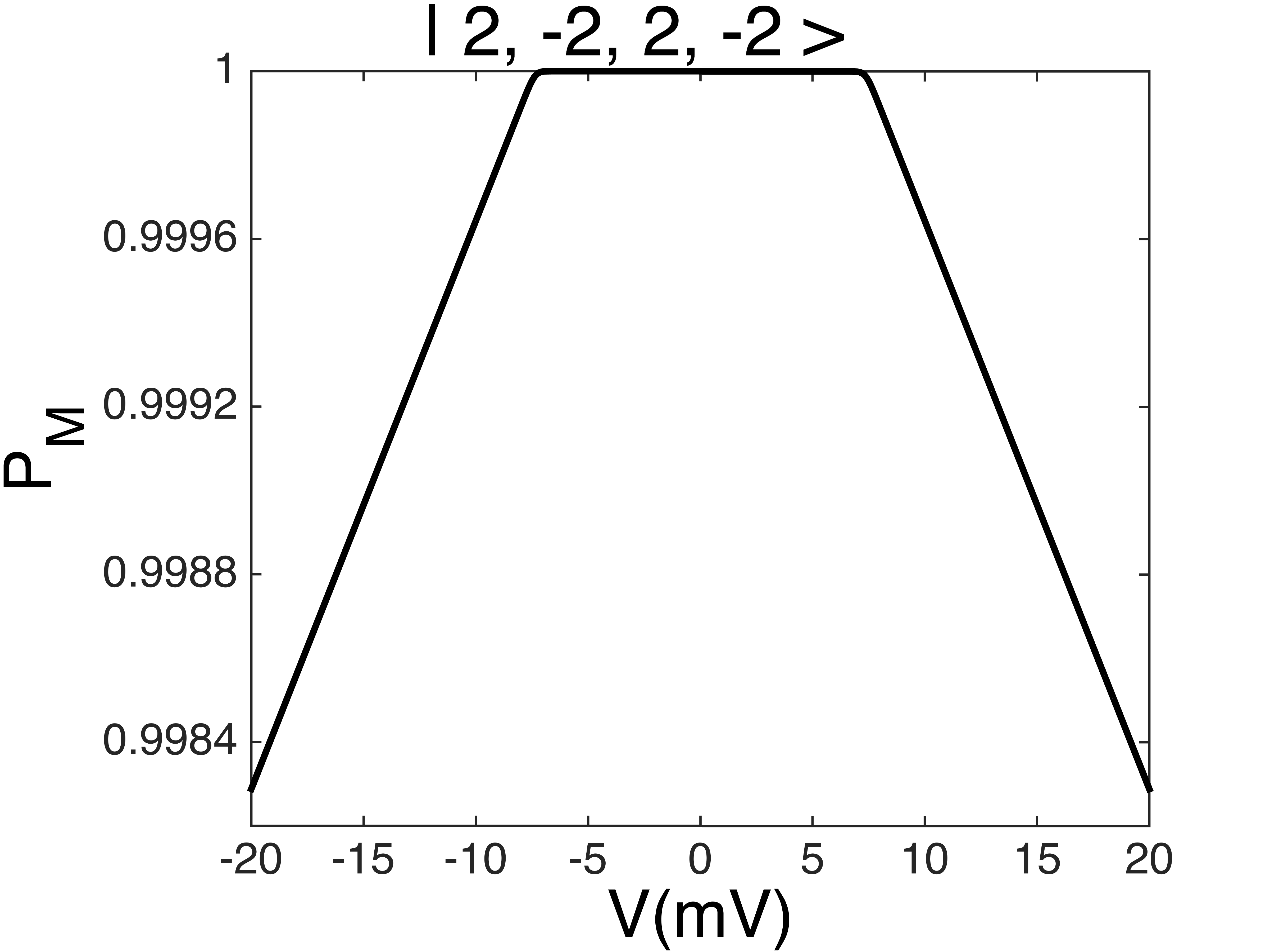
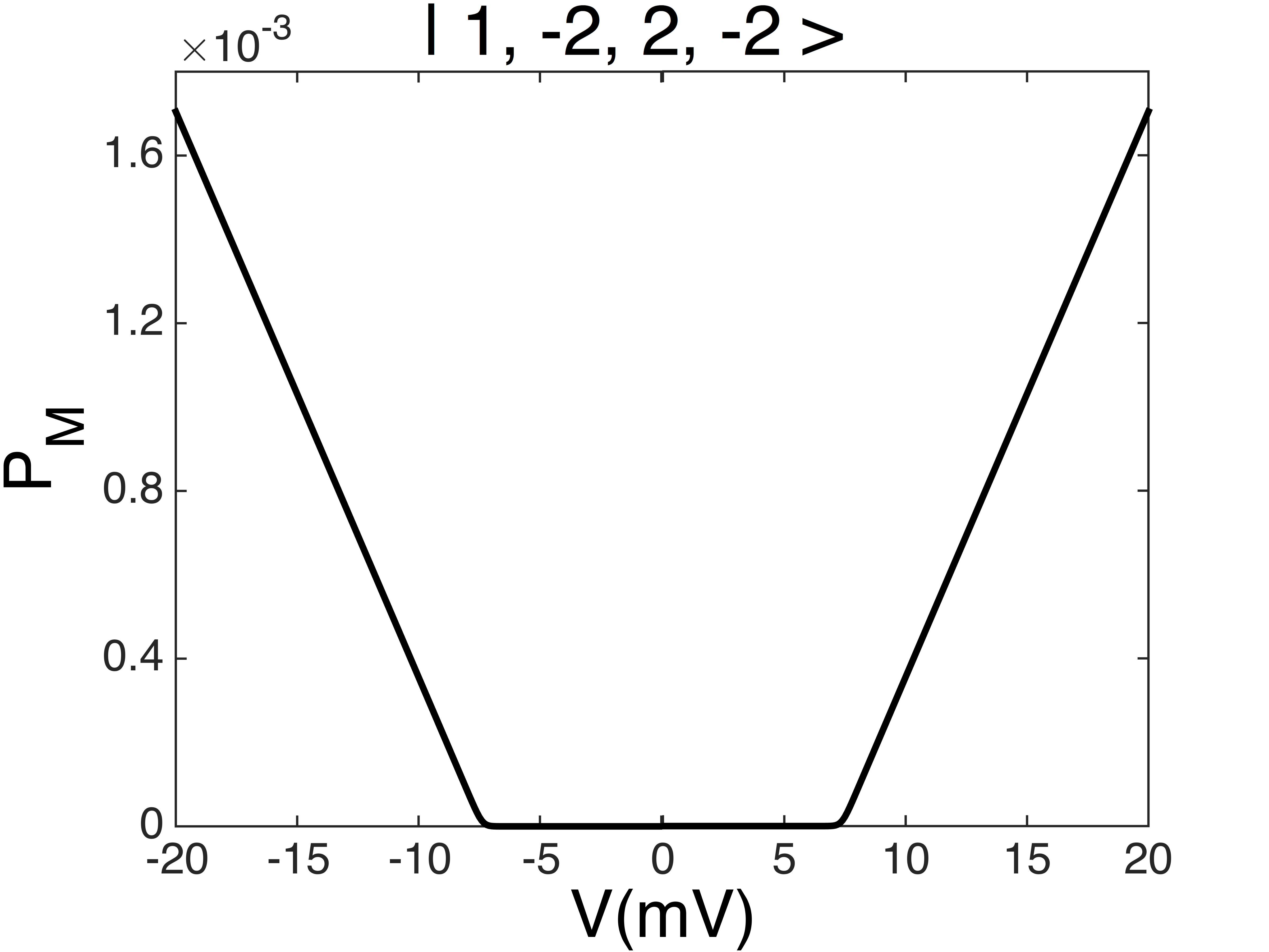
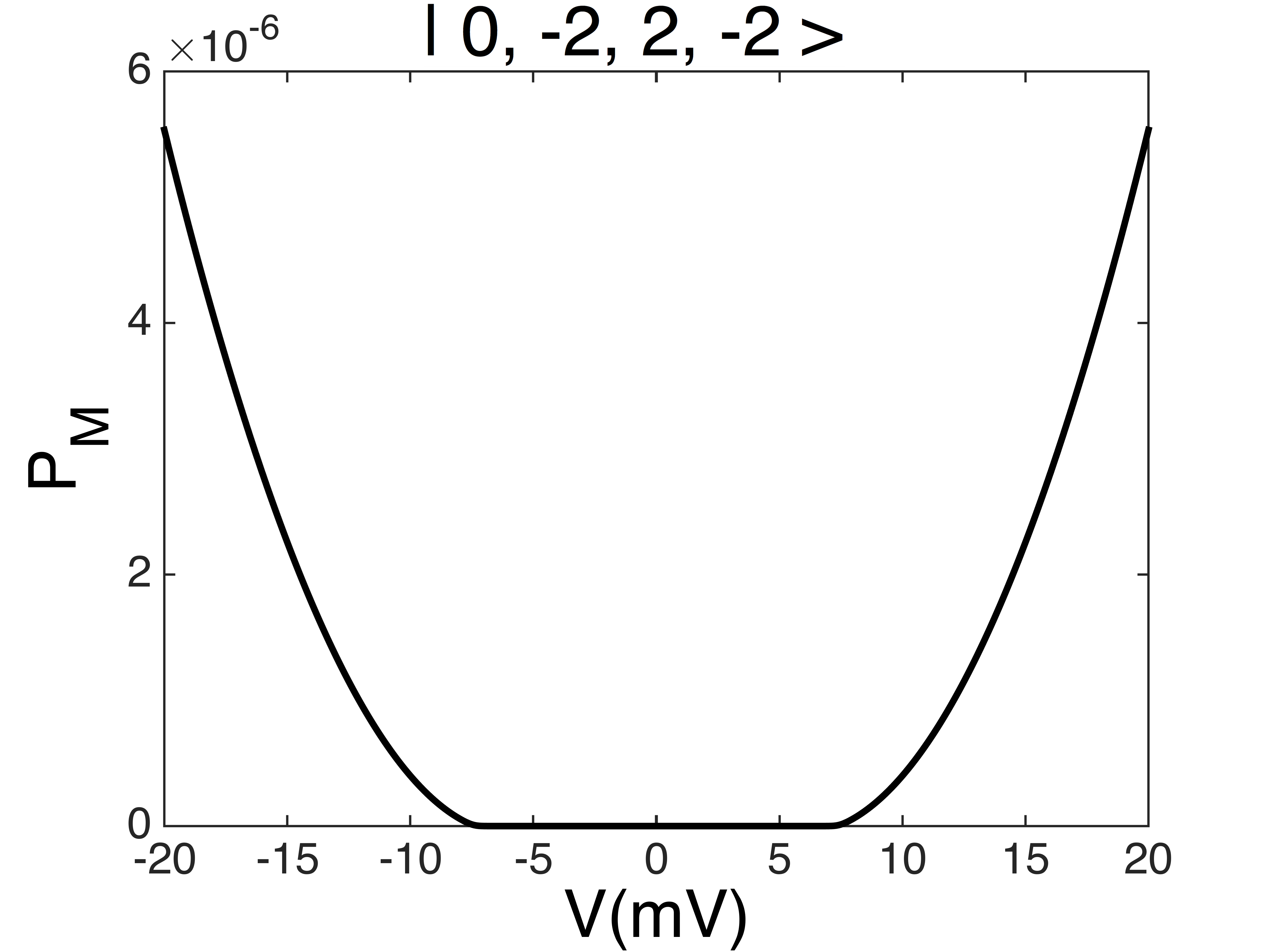
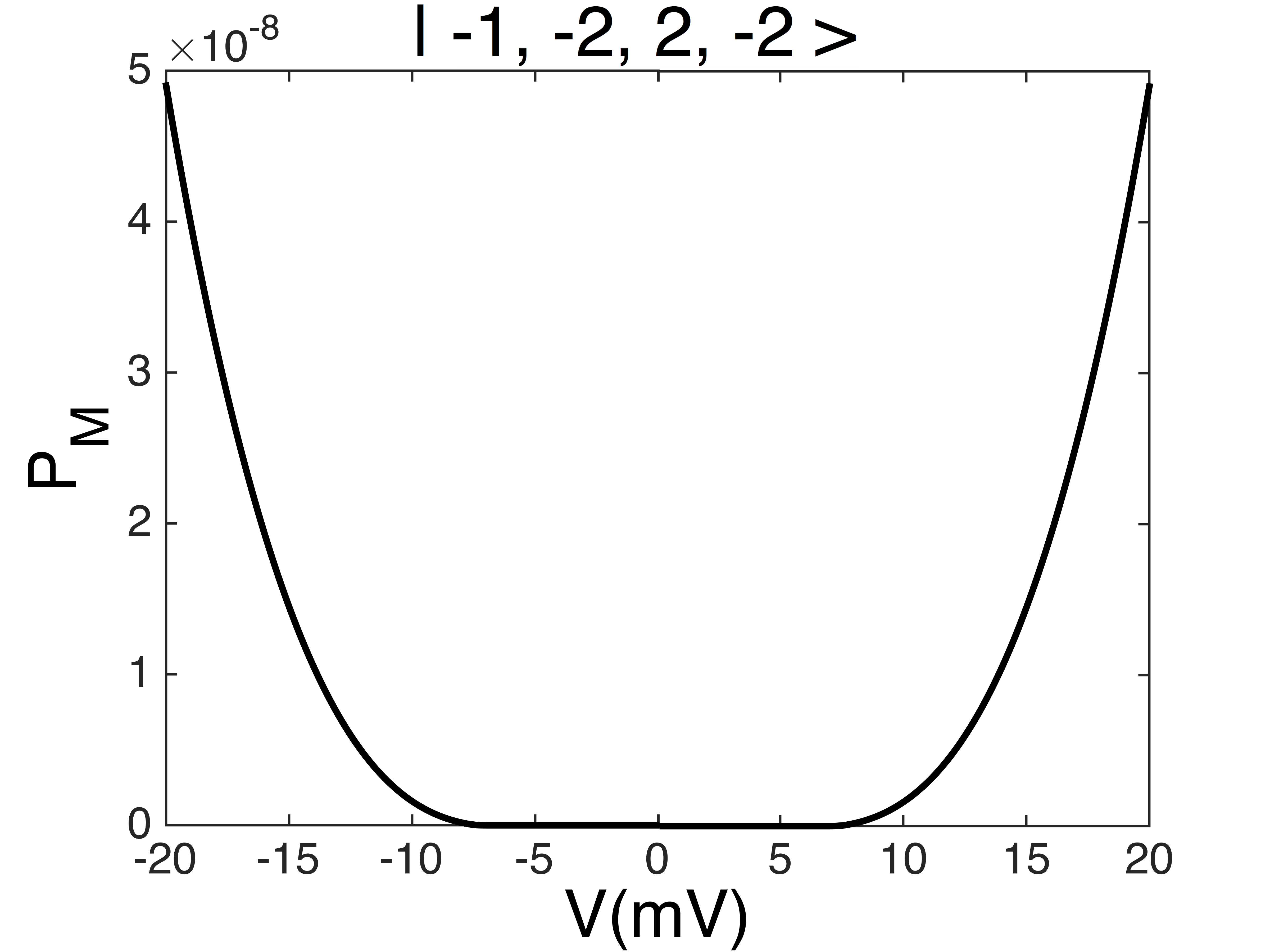
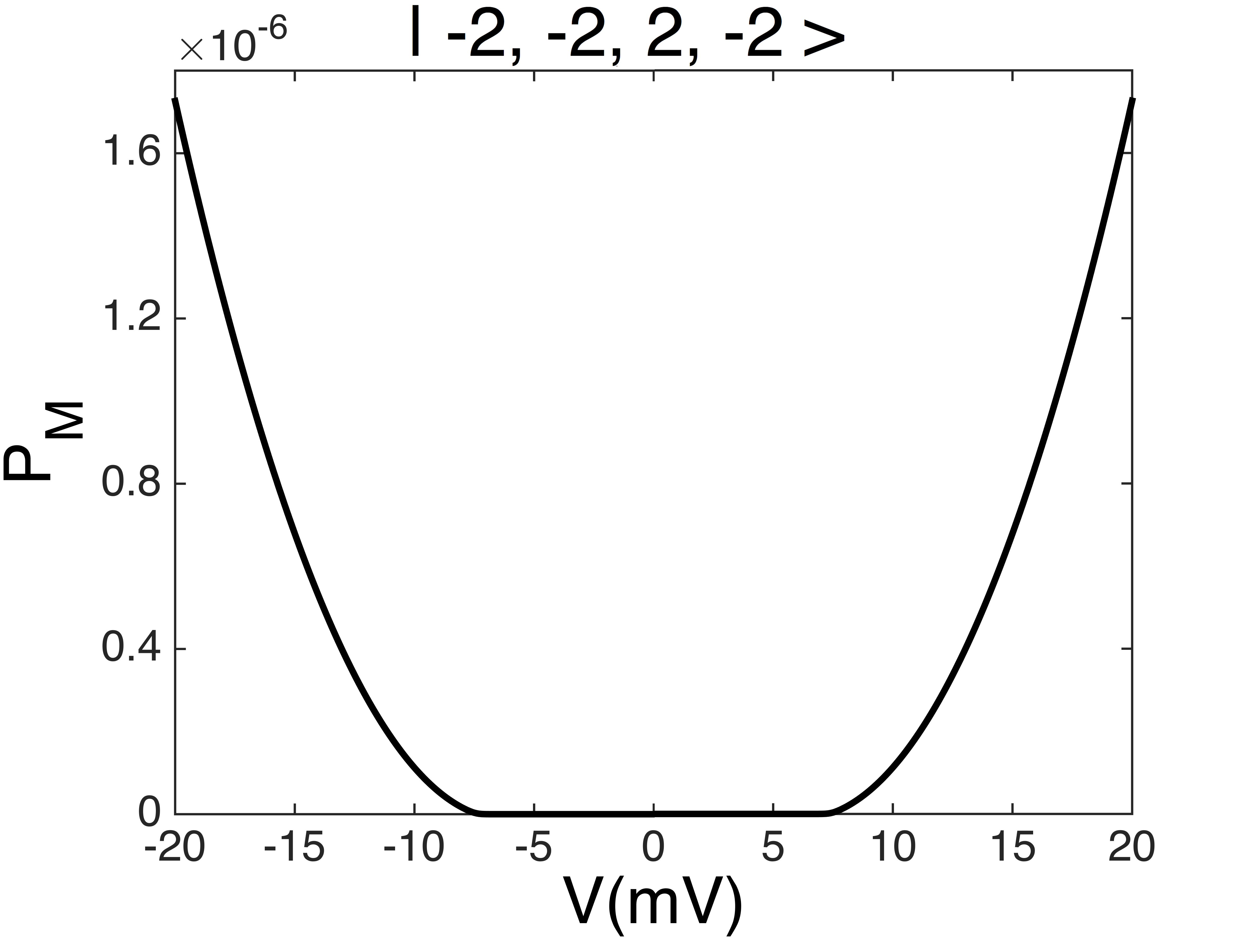
Figure 9: Steady-state population $P_{M}(V)$ as a function of the applied bias voltage of the five eigenstates with $m_{1}\in[2,..,-2]$ of a four-atom antiferromagnetic chain in the ground state (see also Fig. 5). Parameters used are $D=-1.3$  meV, $J=1.7$  meV, $B=1$  T and $T=1$  K.

In this appendix we derive and analyze an analytic expression for the equilibrium population $P_{M}(V)\equiv P_{m_{1},\ldots,m_{N}}(V)$ for $E=0$ (here the label $M=(m_{1},..,m_{N})$ refers to the quantum state $|m_{1},..m_{N}\rangle^{0)}$). When calculating and plotting the current $I(V)$ [Eq. (10)] up to lowest order in $E$, we calculate and include $P_{M}(V)$ up to lowest order in $E$. As the resulting expressions for $P_{M}(V)$ are rather lengthy, we do not include them here, but instead show $P_{M}(V)$ for $E=0$, in order to provide analytical insight into the dependence of $P_{M}$ on the applied bias voltage $V$. We have verified that in the voltage bias range considered in this paper ($\sim 40$ meV) the effect of including nonzero transverse anisotropy in the master equations (30) below is small ($<3\%$), so that the populations $P_{M}(V)$ are to a reasonable approximation given by the solution (33) for $E=0$. $P_{M}(V)$ is the steady-state solution of the master equation delg10 ; delg11 :

$$\frac{dP_{M}(V)}{dt} = \sum_{M^{\prime}}P_{M^{\prime}}(V)W_{M^{\prime},M}(V)\ -$$ (30)

$$\hskip 14.22636ptP_{M}(V)\sum_{M^{\prime}}W_{M,M^{\prime}}(V)=0,$$

with

$$W_{M,M^{\prime}}(V) = \sum_{\stackrel{{\scriptstyle\eta=S}}{{\eta^{\prime}=S,T}}}W_{M,M^{\prime}}^{\eta\to\eta^{\prime}}(V)$$

$$= W_{M,M}^{{\rm S}\,\to\,{\rm T}}(V)+W_{M,M^{\prime}}^{{\rm S}\,\to\,{\rm S}}+W_{M,M^{\prime}}^{{\rm S}\,\to\,{\rm T}}(V).$$

The master equation (30) was derived in Ref. delg11 and relies on the assumptions that $\hbar/(k_{B}T)$, $\hbar/(E_{n}-E_{n^{\prime}})\ll 1/W_{n,n^{\prime}}$, where $\hbar/(k_{B}T)$ is the correlation time of the electrons in the leads, $\hbar/(E_{n}-E_{n^{\prime}})$ the period of coherent evolution and $W_{n,n^{\prime}}$ the scattering time. The three rates in Eq. (LABEL:eq:rates) $W_{M,M}^{{\rm S}\,\to\,{\rm T}}(V)$ (no induced spin flip; spin-independent contribution to the elastic current), $W_{M,M^{\prime}}^{{\rm S}\,\to\,{\rm S}}$ (spin flip, but no contribution to the current) and $W_{M,M^{\prime}}^{{\rm S}\,\to\,{\rm T}}(V)$ (spin-flip, contribution to the inelastic current) are given by Eqns. (18)-(LABEL:eq:WW3) - see also the discussion of these rates and their dependence on $V$ at the beginning of section II.3. We assume the tip-induced exchange couplings $W_{m_{1},..,m_{N}^{\prime}}^{{\rm T}\,\to\,{\rm T}}$ and $W_{m_{1},..,m_{N}^{\prime}}^{{\rm T}\,\to\,{\rm S}}$ to be negligible for $V>0$ as observed in experiments on atomic spin chains spin14 - these rates could, however, straightforwardly be included. Assuming the STM tip to be only coupled to the atom at site $j$, taking $E=0$, and writing $P_{m_{j}}(V)\equiv P_{m_{1},..,m_{j},..,m_{N}}(V)$, Eq. (30) can be written as

$$0 = H_{m_{j}}(V)P_{m_{j}+1}(V)\ +\ K_{m_{j}}(V)P_{m_{j}-1}(V)$$ (32)

$$\ -\ L_{m_{j}}(V)P_{m_{j}}(V).$$

The solution of Eq. (32) is given by:

$$P_{2}(V) = \frac{K_{2}(V)K_{1}(V)K_{0}(V)K_{-1}(V)}{N(V)}\,T_{j}$$

$$P_{1}(V) = \frac{H_{1}(V)K_{1}(V)K_{0}(V)K_{-1}(V)}{N(V)}\,T_{j}$$

$$P_{0}(V) = \frac{H_{1}(V)H_{0}(V)K_{0}(V)K_{-1}(V)}{N(V)}\,T_{j}$$ (33)

$$P_{-1}(V) = \frac{H_{1}(V)H_{0}(V)H_{-1}(V)K_{-1}(V)}{N(V)}\,T_{j}$$

$$P_{-2}(V) = \frac{H_{1}(V)H_{0}(V)H_{-1}(V)H_{-2}(V)}{N(V)}\,T_{j},$$

with

$$N(V) \equiv H_{1}H_{0}H_{-1}H_{-2}+H_{1}H_{0}H_{-1}K_{-1}+$$

$$H_{1}H_{0}K_{0}K_{-1}\,+\,H_{1}K_{1}K_{0}K_{-1}+$$

$$K_{2}K_{1}K_{0}K_{-1}$$

$$H_{m_{j}}(V) = W_{2}\,F_{m_{j},-}(0)\,+\,W_{3}\,F_{m_{j},-}(V)$$

$$K_{m_{j}}(V) = W_{2}\,G_{m_{j},-}(0)\,+\,W_{3}\,G_{m_{j},-}(V)$$

$$L_{m_{j}}(V) = W_{2}\,[F_{m_{j},+}(0)+G_{m_{j},+}(0)]\,+$$

$$\,W_{3}\,[F_{m_{j},+}(V)+G_{m_{j},+}(V)]$$

$$F_{m_{j},s}(V) \equiv C_{m_{j}}\,\frac{eV+s\Delta_{m_{j},F}}{1-\exp{[-\beta(eV+s\Delta_{m_{j},F})]}}$$

$$G_{m_{j},s}(V) \equiv C_{m_{j}-1}\,\frac{eV-s\Delta_{m_{j},G}}{1-\exp{[-\beta(eV-s\Delta_{m_{j},G})]}}$$

$$\Delta_{m_{j},F} \equiv E_{m_{1},...,m_{j},..,m_{N}}-E_{m_{1},...,m_{j}+1,..,m_{N}}$$

$$= -(2m_{j}+1)D\,-\,(m_{j-1}+m_{j+1})J\,+\,E_{Z}$$

$$\Delta_{m_{j},G} \equiv E_{m_{1},...,m_{j}-1,..,m_{N}}-E_{|m_{1},...,m_{j},..,m_{N}}$$

$$= -(2m_{j}-1)D\,-\,(m_{j-1}+m_{j+1})J\,+\,E_{Z}\vspace*{0.5cm}$$

and $C_{m_{j}}$ given by Eq. (15). It is straightforward to verify that Eq. (33) fulfills conservation of population: $\sum_{m_{j}=-2}^{2}P_{m_{j}}(V)\equiv T_{m_{j}}(V)$, where $T_{m_{j}}(V)\equiv T_{m_{1},..,m_{j},..m_{N}}(V)$ $\in[0,1]$ denotes the total (time-independent) spin population of site $j$ for a given set of values $m_{i}$ at the other sites $i\neq j$, and $\sum_{j}T_{j}(V)=1$. Fig. 9 shows the equilibrium population $P_{M}(V)$ [Eq. (33)] for a chain of four antiferromagnetically coupled atoms with population initially in the ground state $|2,-2,2,-2\rangle^{(0)}$ and the STM tip coupled to the first atom. We see that for this initial state and $T_{m_{1}}(V)=1$, corresponding to low temperatures $k_{B}T\ll|\Delta_{1}|$ initially all population is located in the ground state (for larger $k_{B}T>|\Delta_{1}|$ more levels can become occupied, when different $T_{j}$ start to contribute). The ground state population decreases starting at $eV=\pm|\Delta_{1}|$ when the chain can make a transition to the first excited state. However, the population decrease is only slight: at all voltages considered the equilibrium population of the first excited state (or higher excited states) is at least a factor $10^{3}$ smaller than the probability of the chain being in the ground state.

References

- (1) S. Loth et al., Science 335, 196 (2012).
- (2) A.J. Heinrich, J.A. Gupta, C.P. Lutz, and D.M. Eigler, Science 306, 466 (2004).
- (3) C.F. Hirjibehedin, C.P. Lutz and A.J. Heinrich, Science 312, 1021 (2006).
- (4) C.F. Hirjibehedin, C.-Y. Lin, A.F. Otte, M. Ternes, C.P. Lutz, B.A. Bones and A.J. Heinrich, Science 317, 1199 (2007).
- (5) A.F. Otte et al., Nature Physics 4, 847 (2008).
- (6) A. Spinelli et al., Nature Mat. 13, 782 (2014).
- (7) A.A. Khatjetoorians et al, Science 339, 55 (2013).
- (8) S. Yan et al., Nature Nanotechnology 10, 40 (2015).
- (9) J. Fernández-Rossier, Phys. Rev. Lett. 102, 256802 (2009).
- (10) N. Lorente and J.-P. Gauyacq, Phys. Rev. Lett. 103, 176601 (2009); M. Persson, ibid., 050801 (2009).
- (11) B. Sothmann and J. König, New J. Phys. 12, 083028 (2010).
- (12) F. Delgado and J. Fernández-Rossier, Phys. Rev. B 82, 134414 (2010).
- (13) J.-P. Gauyacq and N. Lorente, Phys. Rev. B 87, 195402 (2013).
- (14) J.-P. Gauyacq, S. Moisés Yaro, X. Cartoixà and N. Lorente, Phys. Rev. Lett. 110, 087201 (2013).
- (15) J. Li and B.-G. Liu, J. Phys. D 48, 1 (2015).
- (16) M. Ternes, New J. Phys. 17, 063016 (2015).
- (17) D. Gatteschi, R. Sessoli, and J. Villain, Molecular Nanomagnets, (Oxford University Press, New York, 2006).
- (18) E. Burzurí, R. Gaudenzi, and H.S.J. van der Zant, J. Phys. Cond. Mat. 27, 113202 (2015).
- (19) F. Delgado and J. Fernández-Rossier, Phys. Rev. Lett. 108, 196602 (2012).
- (20) See also, in a different context, D. Jacob and J. Fernández-Rossier, ArXiv:1507.08474, in which the effect of anisotropy on the Kondo effect is discussed.
- (21) M. Misiorny and J. Barnaś, Phys. Rev. Lett. 111, 046603 (2013). See also M. Misiorny and I. Weymann, Phys. Rev. B 90, 235409 (2014).
- (22) B. Bryant, A. Spinelli, J.J.T. Wagenaar, M. Gerrits, and A.F. Otte, Phys. Rev. Lett. 111, 127203 (2013); See also the theoretical investigation of effects of higher-order (multiaxial) anisotropy on the switching probability of a singe quantum spin by C. Hübner, B. Baxevanis, A.A. Khajetoorians, and D. Pfannkuche, Phys. Rev. B 90, 155134 (2014).
- (23) In Ref. gauy13 Gauyacq and Lorente studied the dependence of the magnetic switching time of a chain consisting of a few ferromagnetically coupled atoms on the strength of the transverse magnetic anisotropy. They predicted both a rapid increase of the switching time with and a large dependence of this time on the length of the chain.
- (24) S. Yan, D.-J. Choi, J.A.J. Burgess, S. Rolf-Pissarczyk and S. Loth, Nanoletters 15, 1938 (2015).
- (25) J.C. Oberg, M. Reyes Calvo, F. Delgado, M. Moro-Lagares, D. Serrate, D. Jacob, J. Fernandez-Rossier, C.F. Hirjibehedin, Nature Nanotechnology 9, 64 (2014).
- (26) IETS was first used to investigate and explain molecular vibration spectra by J. Lambe and R.C. Jaklevic, Phys. Rev. 165, 821 (1968) (see also their earlier experiment R.C. Jaklevic and J. Lambe, Phys. Rev. Lett. 17, 1139 (1966)).
- (27) J. Fransson, O. Eriksson, and A. V. Balatsky, Phys. Rev. B 81, 115454 (2010); A. Hurley, N. Baadji and S. Sanvito, Phys. Rev. B 84, 035427 (2011).
- (28) F. Delgado and J. Fernández-Rossier, Phys. Rev. B 84, 045439 (2011).
- (29) Estimates of derived from experimental data for Fe adsorbed on different surfaces are given by F. Delgado, S. Loth, M. Zielinski and J. Fernández-Rossier, Eur. Phys. Lett. 109, 57001 (2015); see also Y.-H. Zhang et al., Nature Communications 4, 1 (2013).
- (30) See e.g. F. Delgado, J.J. Palacios, and J. Fernández-Rossier, Phys. Rev. Lett. 104, 026601 (2010).
- (31) The steplike increase at is not included in the analytic expression (23), where we assumed . Substituting instead the exact stationary solution of , Eq. (33), into Eq. (10) is straightforward and does lead to this step. However, since the resulting expression is somewhat lengthy we have omitted it here.
- (32) S. Loth, K.v. Bergmann, M. Ternes, A.F. Otte, C.P. Lutz, C.F. Hirjibehedin, and A.J. Heinrich, Nature Physics 6, 340 (2010).