Modified interactions in a Floquet topological system on a square lattice
and their impact on a bosonic fractional Chern insulator state

Abstract

We propose a simple scheme for the realization of a topological quasienergy band structure with ultracold atoms in a periodically driven optical square lattice. It is based on a circular lattice shaking in the presence of a superlattice that lowers the energy on every other site. The topological band gap, which separates the two bands with Chern numbers $\pm 1$, is opened in a way characteristic to Floquet topological insulators, namely, by terms of the effective Hamiltonian that appear in subleading order of a high-frequency expansion. These terms correspond to processes where a particle tunnels several times during one driving period. The interplay of such processes with particle interactions also gives rise to new interaction terms of several distinct types. For bosonic atoms with on-site interactions, they include nearest neighbor density-density interactions introduced at the cost of weakened on-site repulsion as well as density-assisted tunneling. Using exact diagonalization, we investigate the impact of the individual induced interaction terms on the stability of a bosonic fractional Chern insulator state at half filling of the lowest band.

I Introduction

The powerful concept of Floquet engineering Goldman and Dalibard (2014); Eckardt and Anisimovas (2015); Goldman et al. (2015); Bukov et al. (2015); Holthaus (2016) is based on the possibility to emulate effective time-independent Hamiltonians with desired properties by subjecting a suitably chosen and well controllable physical system to a time-periodic external field. This procedure relies on the observation that the evolution of a quantum system described by a time-periodic Hamiltonian is governed by a time-independent effective Hamiltonian Rahav et al. (2003); Goldman and Dalibard (2014); Eckardt and Anisimovas (2015); Goldman et al. (2015); Bukov et al. (2015). It is particularly relevant for modern experiments on cold-atom systems in optical lattices Bloch et al. (2008); Dalibard et al. (2011); Lewenstein et al. (2012); Windpassinger and Sengstock (2013); Goldman et al. (2014), which are prominent due to their unsurpassed level of control, nearly perfect structural purity as well as the high degree of isolation and consequent minimal dissipation. Complementing these advantages with a specific driving protocol that allows for a clear physical interpretation of the resulting effective Hamiltonian (computed within a suitable approximation), one is able to carry out quantum simulation of paradigmatic physical models and realize novel or elusive phases of matter. Successful experiments include the demonstration of the basic quantum phase transition between superfluid and Mott-insulating phases Eckardt et al. (2005); Zenesini et al. (2009), emulation of spin models Eckardt et al. (2010); Struck et al. (2011, 2013), realization of intense artificial magnetic fields Aidelsburger et al. (2011); Bermudez et al. (2011); Kolovsky (2011); Aidelsburger et al. (2013, 2015); Struck et al. (2012, 2013); Miyake et al. (2013); Atala et al. (2014); Kennedy et al. (2015), and topological band structures Jotzu et al. (2014); Aidelsburger et al. (2015). In addition to the detection of integrated topological characteristics (Chern numbers), full tomography of the Berry curvature Hauke et al. (2014) has recently been achieved Fläschner et al. .

Concerning topological band structure engineering, it is important to make a clear distinction between “fast” and “intermediate” driving schemes. Here the relevant parameters are the energy scale $\hbar\omega$ defined by the driving frequency $\omega$ and the characteristic energy of the system’s internal degrees of freedom; for lattice systems, typically the hopping parameter $J$. The limit of rapid forcing is defined by the condition $\hbar\omega\gg J$, and the effective Hamiltonian is adequately approximated by the straightforward time average of the driven Hamiltonian. A number of schemes of this type were proposed and realized Eckardt et al. (2005); Lignier et al. (2007); Sias et al. (2008); Zenesini et al. (2009); Alberti et al. (2009); Eckardt et al. (2010); Haller et al. (2010); Struck et al. (2011); Kolovsky (2011); Aidelsburger et al. (2011); Hauke et al. (2012); Struck et al. (2012, 2013); Aidelsburger et al. (2013); Miyake et al. (2013); Jotzu et al. (2014); Atala et al. (2014); Creffield and Sols (2014); Aidelsburger et al. (2015); Kennedy et al. (2015); Fläschner et al. . Going beyond the time-averaging of the driven Hamiltonian one relies on an expansion in powers of the inverse frequency (or, equivalently, the period) Goldman and Dalibard (2014); Eckardt and Anisimovas (2015); Goldman et al. (2015); Bukov et al. (2015); Mikami et al. and includes successive terms proportional to, e. g., $J/\hbar\omega$ and $(J/\hbar\omega)^{2}$. Schemes relying on these contributions have been termed Floquet topological insulators Oka and Aoki (2009); Kitagawa et al. (2010); Lindner et al. (2011); Kitagawa et al. (2011); Cayssol et al. (2013); Grushin et al. (2014) and have been demonstrated not only in an optical lattice Jotzu et al. (2014), but also in photonic wave guides Rechtsman et al. (2013). These subleading terms have a clear physical interpretation Eckardt and Anisimovas (2015); Anisimovas et al. (2015) which is an essential ingredient that makes the term-by-term construction of the effective Hamiltonians meaningful. The relevant corrections are: (a) processes where a particle tunnels twice during a driving period thus generating effective matrix elements for tunneling beyond nearest neighbors, and (b) combined events involving an interplay between kinetics and interactions, which are the main focus of the present manuscript. Both types of processes are intimately related to the presence of a significant micromotion corresponding to the periodic motion of particles in real space at the driving frequency. In a recent study Anisimovas et al. (2015), the coupling of micromotion and interactions was shown to be largely detrimental to the stabilization of the fractional Chern insulator phases Sheng et al. (2011); Neupert et al. (2011); Sun et al. (2011); Regnault and Bernevig (2011); Wang et al. (2011); Wu et al. (2012); Grushin et al. (2014, 2015); Bergholtz and Liu (2013); Parameswaran et al. (2013). However, a detailed analysis and an insight into the underlying mechanism was not given.

The aim of the present paper is twofold: On the one hand we propose a scheme for the realization of a Floquet topological band structure with two Chern bands in a circularly driven square lattice. The scheme reproduces the physics of the chiral $\pi$-flux model Neupert et al. (2011); Sun et al. (2011); Regnault and Bernevig (2011) and relies on engineering the necessary flux configuration by “photon”-assisted hoppings in the presence of sublattice modulation, while the topological band gaps are opened due to induced next-neareast neighbor transitions. On the other hand, we investigate the stability of the fractional Chern insulator phase Bergholtz and Liu (2013); Parameswaran et al. (2013) of bosonic particles in the half-filled lowest energy band. In particular, we focus on the impact of different micromotion-induced interaction terms Eckardt and Anisimovas (2015); Anisimovas et al. (2015) in the effective Hamiltonian, investigating in detail which of these terms are beneficial and which detrimental for the preparation of the fractional Chern insulator state.

We find that micromotion-induced corrections to particle interactions can be separated into three constituent components: (i) weakening of the on-site interaction strength, (ii) the appearance of induced interactions between neighboring sites even if they were absent in the original model, and (iii) the remaining density-assisted tunneling events. Interestingly, contributions of density-density interaction type, (i) and (ii), satisfy a constraint in the form of a sum rule indicating that the diminished on-site interaction energy is precisely compensated by the corresponding increase of nearest-neighbor interaction energies; in other words, the interactions are “smeared out” by micromotion. We study the impact of the three effects on the stability of the fractional Chern insulator phase and demonstrate that, as the driving frequency becomes lower, this phase is primarily destabilized by the destructive role of the density-assisted hopping terms.

Our paper has the following structure. In Sec. II, we present a feasible scheme of practical realization of the chiral $\pi$-flux model supporting robust topological single-particle energy bands. The inclusion of inter-particle interactions and their coupling to the real-space micromotion are discussed in Sec. III and supported with numerical results in Sec. IV. We summarize our findings in the concluding Sec. V, while a number of issues of technical nature are delegated to Appendices. The topics include the creation of artificial gauge structures, high-frequency expansion of the effective Hamiltonian, and supplemental analysis of single-particle band structures.

II Modulated square lattice

In this section, we describe a specific driving scheme that allows to realize the chiral $\pi$-flux model Neupert et al. (2011); Sun et al. (2011); Regnault and Bernevig (2011) on a modulated square lattice. As the name implies, this model features elementary plaquettes pierced by (artificial) magnetic fluxes equal to one half of the dimensionless flux quantum $2\pi$. Alongside with the Haldane model Haldane (1988); Alba et al. (2011); Goldman et al. (2013) based on a hexagonal lattice, the chiral $\pi$-flux model presents an unpretentious two-band configuration that serves as a basis for robust topological band structures. In the presence of only nearest-neighbor hopping both models support band structures featuring two Dirac points where the upper and the lower bands touch at a singular point in a cone-like fashion. Inclusion of next-nearest neighbor transitions leads to the opening of topological band gaps whereby the two energy bands separate and may acquire the Chern indices of $\pm 1$. The presence of additional tunable parameters (essentially, the ratio of nearest and next-nearest neighbor transition strengths) allows one to tune into the regime where topological bands are relatively flat in comparison to band gaps and interaction energies. These circumstances pave the wave towards the realization of so far elusive fractional Chern insulators.

II.1 Driven Hamiltonian and flux configuration

In order to produce the required flux configuration, we start from a static square lattice of spacing $d$ shown in Fig. 1 (a). Here, the full blue lines denote nearest-neighbor links characterized by a spatially uniform bare tunneling parameter $J$. Next, we bipartition the original lattice into two square sublattices $\mathcal{A}$ and $\mathcal{B}$ with lattice constants $\sqrt{2}d$, intertwined in a checkerboard fashion. By means of lowering the on-site energies on sublattice $\mathcal{B}$ by the quantity $\hbar\omega$, the natural hopping transitions between nearest-neighbor sites are inhibited and must be assisted by an external driving at frequency $\omega$. The resulting lattice configuration is shown in Fig. 1 (b) with dashed blue lines indicating such “photon”-assisted transitions.

The effects of a time-periodic lattice forcing are captured by the driven single-particle Hamiltonian

$$\hat{H}(t)=-J\sum_{\langle ij\rangle}\hat{a}^{{\dagger}}_{i}\hat{a}_{j}+\sum_{i}v_{i}(t)\hat{a}^{{\dagger}}_{i}\hat{a}_{i},$$ (1)

with the lattice degrees of freedom encoded by annihilation (creation) operators $\hat{a}_{i}^{({\dagger})}$. The Hamiltonian (1) is composed of the static part representing transitions on all directed lattice links $\langle ij\rangle$ plus the driving term featuring time- and coordinate-dependent on-site potentials $v_{i}(t)$. In the case of circular driving by a rotating force of magnitude $F$ and on-site energy offsets $(-\hbar\omega)$ affecting only sublattice $\mathcal{B}$, a further gauge transformation (see Appendix A for details) leads to the purely kinetic driven Hamiltonian in the form

$$\hat{H}(t)=-\sum_{i\in\mathcal{A}}\sum_{\mu=1}^{4}J_{\mu}(t)\,\hat{b}^{{\dagger}}_{i+\mu}\hat{a}_{i}+\mathrm{h.c.},$$ (2)

with $\hat{a}_{i}^{({\dagger})}$ and $\hat{b}_{i}^{({\dagger})}$ denoting the annihilation (creation) operators defined on the respective sublattices. In order to count all nearest-neighbor connections only once, we sum over all sites belonging to the sublattice $\mathcal{A}$ and over the four distinct directions $\bm{\delta}_{\mu}$ (see Fig. 1 for definitions) linking to the nearest neighbors belonging to the sublattice $\mathcal{B}$. The time-dependent hopping parameters are given by [cf. (43)]

$$J_{\mu}(t)=J\,\mathrm{e}^{\mathrm{i}\alpha\sin(\omega t-\varphi_{\mu})}\mathrm{e}^{-\mathrm{i}\omega t},$$ (3)

with the scaled shaking strength $\alpha=Fd/\hbar\omega$ and the lagging phases

$$\varphi_{\mu}=\frac{\pi(\mu-1)}{2}=\Big{\{}0,\frac{\pi}{2},\pi,\frac{3\pi}{2}\Big{\}}.$$ (4)

The presence of the exponential factor $\mathrm{e}^{-\mathrm{i}\omega t}$ in the hopping parameter (3) results from the sublattice energy mismatch. We see that the time dependence enters the driven Hamiltonian (2) only through the modulation of the hopping parameters whose Fourier series read

$$J_{\mu}(t)=\sum_{s=-\infty}^{\infty}J\mathcal{J}_{1+s}(\alpha)\,\mathrm{e}^{-\mathrm{i}(1+s)\varphi_{\mu}}\,\mathrm{e}^{\mathrm{i}s\omega t},$$ (5)

with $\mathcal{J}_{m}(x)$ denoting the Bessel function of the first kind and order $m$. In the high-frequency limit, when time averaging of the driven Hamiltonian is an adequate approximation, one has

$$\langle J_{\mu}(t)\rangle_{T}=J\mathcal{J}_{1}(\alpha)\,\mathrm{e}^{-\mathrm{i}\varphi_{\mu}},$$ (6)

so that the Peierls phases associated with transitions from sublattice $\mathcal{A}$ to sublattice $\mathcal{B}$ are given by the lagging phases (4). Keeping in mind that transitions in the opposite direction are associated with complex conjugate matrix elements and inverted phases, it is easy to check that the total phase accumulated while travelling around each square plaquette equals

$$-\frac{\pi}{4}+\frac{3\pi}{4}-\frac{5\pi}{4}+\frac{7\pi}{4}=\pi.$$

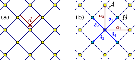
Figure 1: Realizing the chiral-$\pi$ model. The original square lattice in panel (a) is separated into two energy-mismatched sublattices (yellow $\mathcal{A}$ and cyan $\mathcal{B}$) of a larger lattice constant in panel (b). The vectors $\bm{\delta}_{\mu}$ with $\mu=\{1,2,3,4\}$ connect the nearest-neighbor sites belonging to distinct sublattices. The vectors $\bm{a}_{1|2}$ are the elementary translation vectors. Full (dashed) blue lines depict natural (driving-assisted) transitions.

II.2 Description in quasimomentum space

To proceed with further analysis, it is convenient to switch into the reciprocal space, which is accomplished through the introduction of the quasimomentum-dependent operators

$$\hat{a}^{{\dagger}}_{\bm{k}} =\frac{1}{\sqrt{N_{s}}}\sum_{i\in\mathcal{A}}\hat{a}^{{\dagger}}_{i}\,\mathrm{e}^{\mathrm{i}\bm{k}\cdot\bm{r}_{i}},$$ (7a)

$$\hat{b}^{{\dagger}}_{\bm{k}} =\frac{1}{\sqrt{N_{s}}}\sum_{j\in\mathcal{B}}\hat{b}^{{\dagger}}_{j}\,\mathrm{e}^{\mathrm{i}\bm{k}\cdot(\bm{r}_{j}-\bm{\delta}_{1})}.$$ (7b)

Here $N_{s}$ is the number of sites in a given sublattice. On the second line, the sum runs over all sites $j$ belonging to the sublattice $\mathcal{B}$, and the vector $\bm{r}_{j}$ points to the position of a particular site. The additional shift of its effective position by $\bm{\delta}_{1}$ is included to obtain a $\bm{k}$-periodic Hamiltonian Regnault and Bernevig (2011). Since the driven Hamiltonian (2) only couples sites belonging to different sublattices, we find

$$\hat{H}(t)=-J\sum_{\bm{k}}\hat{b}^{{\dagger}}_{\bm{k}}\hat{a}_{\bm{k}}\,g(t,\bm{k})-J\sum_{\bm{k}}\hat{a}^{{\dagger}}_{\bm{k}}\hat{b}_{\bm{k}}\,g^{*}(t,\bm{k}),$$ (8)

with the matrix element $g(t,\bm{k})$ encompassing the summation over the four nearest-neighbor links

$$\begin{split}g(t,\bm{k})&=\sum_{\mu=1}^{4}\left[J_{\mu}(t)/J\right]\,\mathrm{e}^{-\mathrm{i}\bm{k}\cdot(\bm{\delta}_{\mu}-\bm{\delta}_{1})}\\ &=\sum_{s=-\infty}^{\infty}\mathcal{J}_{1+s}(\alpha)G_{1+s}(\bm{k})\,\mathrm{e}^{\mathrm{i}s\omega t}.\end{split}$$ (9)

Here, we found it convenient to introduce a family of auxiliary functions

$$\begin{split}G_{s}(\bm{k})&=1+\mathrm{e}^{-\mathrm{i}s\pi/2}\mathrm{e}^{\mathrm{i}\bm{k}\cdot\bm{a}_{1}}\\ &+\mathrm{e}^{\mathrm{i}s\pi}\mathrm{e}^{\mathrm{i}\bm{k}\cdot(\bm{a}_{1}+\bm{a}_{2})}+\mathrm{e}^{\mathrm{i}s\pi/2}\mathrm{e}^{\mathrm{i}\bm{k}\cdot\bm{a}_{2}},\end{split}$$ (10)

whose properties are analyzed in Appendix C. Finally, the operator-valued Fourier coefficients of the driven kinetic Hamiltonian are given by

$$\begin{split}\hat{H}_{s}=&-J\mathcal{J}_{1+s}(\alpha)\sum_{\bm{k}}\hat{b}^{{\dagger}}_{\bm{k}}\hat{a}_{\bm{k}}G_{1+s}(\bm{k})\\ &-J\mathcal{J}_{1-s}(\alpha)\sum_{\bm{k}}\hat{a}^{{\dagger}}_{\bm{k}}\hat{b}_{\bm{k}}G_{1-s}^{*}(\bm{k}).\end{split}$$ (11)

II.3 Effective Hamiltonian

For a periodically driven system, the quantum-mechanical time-evolution operator between arbitrary times $t_{1}$ and $t_{2}$ can be factorized like (see, e. g., Goldman and Dalibard (2014); Goldman et al. (2015); Eckardt and Anisimovas (2015); Bukov et al. (2015))

$$\hat{U}(t_{2},t_{1})=\hat{U}_{F}(t_{2})\,\mathrm{e}^{-\mathrm{i}\hat{H}_{F}(t_{2}-t_{1})/\hbar}\hat{U}_{F}^{{\dagger}}(t_{1}).$$ (12)

Here, $\hat{U}_{F}(t)$ is the time-periodic micromotion operator and $\hat{H}_{F}$ is the effective Hamiltonian, which in addition to being stationary is also free from any parametric dependence on the choice of the initial and final instants of time. In this way the effects of micromotion are clearly separated from the effective long-term dynamics. The effective Hamiltonian can be systematically approximated in terms of series in the inverse driving frequency (see Appendix B for details). In the present section, we focus on the single-particle properties and thus restrict our attention to a two-term approximation of the effective Hamiltonian

$$\begin{split}\hat{H}_{F}^{[2]}&=\hat{H}_{F}^{(1)}+\hat{H}_{F}^{(2)}\\ &=\hat{H}_{0}+\frac{1}{\hbar\omega}\sum_{s=1}^{\infty}\frac{1}{s}\big{[}\hat{H}_{s},\hat{H}_{-s}\big{]}.\end{split}$$ (13)

Third-order terms contained in $\hat{H}_{F}^{(3)}$ (47c) are relevant for the coupling between kinetics and interactions, and will be included in the subsequent Sec. III.

II.4 Single-particle spectra

At each point $\bm{k}$ in the Brillouin zone the Hamiltonian $\hat{H}_{F}^{[2]}(\bm{k})$ defines a two-level system, and therefore, is represented by a dot product of a three-dimensional Bloch vector $\mathbf{h}(\bm{k})=\{h_{x}(\bm{k}),h_{y}(\bm{k}),h_{z}(\bm{k})\}$ and the vector of Pauli matrices $\{\sigma_{x},\sigma_{y},\sigma_{z}\}$:

$$\hat{H}_{F}^{[2]}(\bm{k})=\mathbf{h}(\bm{k})\cdot\bm{\sigma}.$$ (14)

The lowest-order contribution to the effective Hamiltonian is given by the time-average of the driven Hamiltonian, or in other words, by its zeroth Fourier component, hence

$$H_{F}^{(1)}=-J\mathcal{J}_{1}(\alpha)\sum_{\bm{k}}\hat{b}^{{\dagger}}_{\bm{k}}\hat{a}_{\bm{k}}G_{1}(\bm{k})+\mathrm{h.c.}.$$ (15)

This term contributes only to off-diagonal components $h_{x}(\bm{k})$ and $h_{y}(\bm{k})$. Obviously, the overall band width is modulated by the Bessel function $\mathcal{J}_{1}(\alpha)$, and the energy spectrum consists of two mirror-symmetric bands given by

$$\varepsilon_{\pm}(\bm{k})=\pm J\left|\mathcal{J}_{1}(\alpha)\right|\left|G_{1}(\bm{k})\right|.$$ (16)

The analysis of the properties of the function $G_{1}(\bm{k})$ presented in Appendix C reveals the presence of two Dirac points, where $h_{x}=h_{y}=0$ and both bands touch in a conical fashion. One Dirac point is situated at the center of the Brillouin zone,

$$\mathrm{D}_{1}:(k_{1}=0,k_{2}=0),$$

and the other one is at a corner of the square-shaped Brillouin zone,

$$\mathrm{D}_{2}:\left(k_{1}=\tfrac{1}{2},k_{2}=\tfrac{1}{2}\right).$$

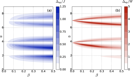
Figure 2: The single-particle band structure of the driven square lattice versus the scaled inverse driving frequency $\beta$ and the scaled driving strength $\alpha$. Panel (a) shows the width of the topological band gap $\Delta_{\textrm{sp}}$ (when present) measured in units of the hopping parameter $J$. In panel (b), the band gap is compared to the width of a single band thus defining the band flatness ratio $\mathscr{F}=\Delta_{\textrm{sp}}/W$.

Proceeding to include the driving-induced second-order hopping transitions, we evaluate the commutators

$$\begin{split}\big{[}\hat{H}_{s},\hat{H}_{-s}\big{]}&=J^{2}\sum_{\bm{k}}\left(\hat{a}^{{\dagger}}_{\bm{k}}\hat{a}_{\bm{k}}-\hat{b}^{{\dagger}}_{\bm{k}}\hat{b}_{\bm{k}}\right)\Big{\{}\mathcal{J}_{s-1}^{2}(\alpha)\left|G_{1-s}(\bm{k})\right|^{2}\\ &-\mathcal{J}_{1+s}^{2}(\alpha)\left|G_{1+s}(\bm{k})\right|^{2}\Big{\}}.\end{split}$$ (17)

These corrections are diagonal in the subband index and thus connect a given site to its next-nearest neighbors as well as further sites belonging to the same sublattice. Note, that the mirror symmetry between the lower and upper energy bands is preserved and the second order correction $\hat{H}_{F}^{(2)}(\bm{k})$ has only $h_{z}(\bm{k})$ component.

The Pauli-matrix representation makes the study of the topological nature of the bands straightforward: For the two energy bands to acquire nontrivial Chern numbers $\pm 1$, the Bloch vector $\mathbf{h}(\bm{k})$ must wrap around the full Bloch sphere Alba et al. (2011); Sticlet et al. (2012); Goldman et al. (2013) visiting its both poles. Consequently, to open a topological band gap $h_{z}(\bm{k})$ should have opposite signs at the two Dirac points. From Eq. (17) we infer (see also Appendix C) that at the Dirac points $\mathrm{D}_{1|2}$, the contributions of the second-order expansion term $\hat{H}_{F}^{(2)}$ are given by an overall prefactor $16J^{2}/\hbar\omega$ times the $\alpha$-dependent oscillatory factors; at $\mathrm{D}_{1}$

$$\mathcal{J}_{0}^{2}(\alpha)-\left(\tfrac{1}{3}-\tfrac{1}{5}\right)\mathcal{J}_{4}^{2}(\alpha)-\left(\tfrac{1}{7}-\tfrac{1}{9}\right)\mathcal{J}_{8}^{2}(\alpha)-\ldots,$$ (18a)

and at $$\mathrm{D}_{2}$$

$$-\left(1-\tfrac{1}{3}\right)\mathcal{J}_{2}^{2}(\alpha)-\left(\tfrac{1}{5}-\tfrac{1}{7}\right)\mathcal{J}_{6}^{2}(\alpha)-\ldots.$$ (18b)

For most values of $\alpha$, the factors (18a) and (18b) have opposite signs that conspire with opposite chiralities of the Dirac points to produce a topological band gap. Exceptions occur only in close vicinity of the zeros of $\mathcal{J}_{0}(\alpha)$; here subleading terms of Eq. (18a) take over and the band structure features a trivial gap. The single-particle band structure generated by the two-term expansion $\hat{H}_{F}^{[2]}$ in Eq. (13) is plotted in Fig. 2 as a function of the scaled inverse driving frequency

$$\beta=\frac{J}{\hbar\omega},$$ (19)

and the scaled driving strength

$$\alpha=\frac{Fd}{\hbar\omega}.$$ (20)

In the left panel the shades of blue indicate the size of the topological gap, if present, that separates the upper and lower energy bands characterized by the Chern indices $\pm 1$. To be fully precise here, the band gap $\Delta_{\textrm{sp}}$ is defined as the global gap, that is

$$\begin{split}\Delta_{\text{sp}}&=\operatorname*{min}_{\bm{k}\in\text{BZ}}\varepsilon_{+}(\bm{k})-\operatorname*{max}_{\bm{k}\in\text{BZ}}\varepsilon_{-}(\bm{k}).\end{split}$$ (21)

Owing to the mirror-symmetry of the energy bands, the band gap is direct. The band gap is of the order $J^{2}/\hbar\omega$ and, thus, vanishes for small $\beta$. This indicates that our scheme belongs to those working at intermediate rather than large driving frequencies. The right panel of Fig. 2 shows the band flatness defined as the ratio of the topological band gap to the overall width of a single band, viz.

$$\mathscr{F}=\frac{\Delta_{\text{sp}}}{W},\qquad W=\operatorname*{max}_{\bm{k}\in\text{BZ}}\varepsilon_{+}(\bm{k})-\operatorname*{min}_{\bm{k}\in\text{BZ}}\varepsilon_{+}(\bm{k}).$$

This quantity is more relevant in the context of stabilization of the fractional Chern insulator phases, ideally requiring topological band gaps exceeding (or at least comparable to Grushin et al. (2015); Kourtis et al. (2014)) the interaction strengths which, in their own turn, must dominate the band width. We see that robust flatness ratios in excess of $4$ can be reached.

III Interplay of micromotion and interactions

In order to gain insight into the effect of coupling between particle tunneling and interaction events that appear in the third-order of the effective Hamiltonian (47c), we consider here a generic situation described by a driven kinetic Hamiltonian

$$\hat{H}(t)=-J\sum_{\langle ij\rangle}\mathrm{e}^{\mathrm{i}\theta_{ij}(t)}\,\hat{a}^{{\dagger}}_{i}\hat{a}_{j},$$ (22)

with Peierls phases of the form (43)

$$\theta_{ij} =\alpha\sin(\omega t-\varphi_{ij})+s_{ij}\,\omega t.$$ (23)

In contrast to the $\bm{k}$-space computational approach taken in the previous Sec. II, we now write the Fourier components of the Hamiltonian (22) in the real space

$$\hat{H}_{s}=-J\sum_{\langle ij\rangle}\mathcal{J}(s-s_{ij}|\alpha)\,\mathrm{e}^{-\mathrm{i}(s-s_{ij})\varphi_{ij}}\hat{a}^{{\dagger}}_{i}\hat{a}_{j}.$$ (24)

Here, in order to avoid the clumsiness of double subscripts we introduced an in-line notation for the Bessel functions $\mathcal{J}(s|\alpha)\equiv\mathcal{J}_{s}(\alpha)$. Let us next assume that interactions between particles are bosonic and on-site, i. e.,

$$\hat{H}_{\text{int}}=\frac{U}{2}\sum_{i}\hat{a}^{{\dagger}}_{i}\hat{a}^{{\dagger}}_{i}\hat{a}_{i}\hat{a}_{i},$$ (25)

and evaluate the nested commutator that defines the third-order contribution to the effective Hamiltonian

$$\begin{split}\big{[}\big{[}\hat{H}_{\text{int}},\hat{H}_{s}\big{]},\hat{H}_{-s}\big{]}&=\frac{UJ^{2}}{2}\sum_{i}\sum_{\langle jk\rangle}\sum_{\langle\ell m\rangle}\big{[}\big{[}\hat{a}^{{\dagger}}_{i}\hat{a}^{{\dagger}}_{i}\hat{a}_{i}\hat{a}_{i},\hat{a}^{{\dagger}}_{j}\hat{a}_{k}\big{]},\hat{a}^{{\dagger}}_{\ell}\hat{a}_{m}\big{]}\\ &\times\mathcal{J}(s-s_{jk}|\alpha)\mathcal{J}(-s-s_{\ell m}|\alpha)\,\mathrm{e}^{-\mathrm{i}(s-s_{jk})\varphi_{jk}}\,\mathrm{e}^{-\mathrm{i}(-s-s_{\ell m})\varphi_{\ell m}}.\end{split}$$ (26)

Focusing on the basic structural element in this expression we obtain

$$\begin{split}\big{[}\big{[}\hat{a}^{{\dagger}}_{i}\hat{a}^{{\dagger}}_{i}\hat{a}_{i}\hat{a}_{i},\hat{a}^{{\dagger}}_{j}\hat{a}_{k}\big{]},\hat{a}^{{\dagger}}_{\ell}\hat{a}_{m}\big{]}&=2\delta_{ij}\delta_{i\ell}\,\hat{a}^{{\dagger}}_{i}\hat{a}^{{\dagger}}_{i}\hat{a}_{k}\hat{a}_{m}+2\delta_{ik}\delta_{im}\,\hat{a}^{{\dagger}}_{j}\hat{a}^{{\dagger}}_{\ell}\hat{a}_{i}\hat{a}_{i}\\ &-4\delta_{ij}\delta_{im}\,\hat{a}^{{\dagger}}_{\ell}\hat{a}^{{\dagger}}_{i}\hat{a}_{i}\hat{a}_{k}-4\delta_{ik}\delta_{i\ell}\,\hat{a}^{{\dagger}}_{j}\hat{a}^{{\dagger}}_{i}\hat{a}_{i}\hat{a}_{m}\\ &+2\delta_{ij}\delta_{k\ell}\,\hat{a}^{{\dagger}}_{i}\hat{a}^{{\dagger}}_{i}\hat{a}_{i}\hat{a}_{m}+2\delta_{ik}\delta_{jm}\,\hat{a}^{{\dagger}}_{\ell}\hat{a}^{{\dagger}}_{i}\hat{a}_{i}\hat{a}_{i}.\end{split}$$ (27)

The individual terms in this result admit a clear physical interpretation (see also Refs. Eckardt and Anisimovas, 2015; Anisimovas et al., 2015). We easily recognize that the first line of Eq. (27) lists pair hopping events: Two particles are removed from site $i$ and placed onto two of its nearest-neighboring sites (either the same site or two distinct sites). The conjugate version allows two particles to hop onto site $i$ from its two neighboring sites. The second line of Eq. (27) introduces density-assisted hopping events between two nearest neighbors of site $i$ using site $i$ as the intermediate stop. If the two nearest neighbors coincide, however, these terms transform into the ordinary density-density interactions between nearest neighbors. Finally, the third and last line lists events where a particle leaves a given site $i$ and travels to another site reachable by two nearest-neighbor transitions. If the origin and the destination coincide, these contributions degenerate into the ordinary on-site repulsion. As we will see shortly, these contributions are negative in the sense that the original on-site repulsion energy $U$ is effectively reduced.

Summarizing the above observations, we note that various contributions induced by combining kinetic and interaction events can be categorized into three classes: (i) terms contributing to the modification of the on-site repulsion energy $U$, (ii) terms leading to the introduction of hitherto absent density-density interaction between nearest neighbor sites, and (iii) more exotic density-assisted and pair tunneling events. It is quite remarkable that the two former contributions obey a constraint that can be interpreted as a conservative partial spread of on-site interactions onto the nearest-neighbor interactions.

In order to demonstrate the advertised result, we review the commutators in Eq. (27) and collect only the terms that contribute to (the reduction of) on-site interactions and obtain

$$\begin{split}&\big{[}\big{[}\hat{a}^{{\dagger}}_{i}\hat{a}^{{\dagger}}_{i}\hat{a}_{i}\hat{a}_{i},\hat{a}^{{\dagger}}_{j}\hat{a}_{k}\big{]},\hat{a}^{{\dagger}}_{\ell}\hat{a}_{m}\big{]}_{\textrm{R}}\\ &\qquad=2\left(\delta_{ij}\delta_{k\ell}\delta_{im}+\delta_{ik}\delta_{jm}\delta_{i\ell}\right)\hat{a}^{{\dagger}}_{i}\hat{a}^{{\dagger}}_{i}\hat{a}_{i}\hat{a}_{i}.\end{split}$$ (28)

Here, the subscript R refers to renormalization of the original on-site repulsion energy. Likewise, filtering out terms that contribute to the appearance of a nearest-neighbor repulsion we obtain

$$\begin{split}&\big{[}\big{[}\hat{a}^{{\dagger}}_{i}\hat{a}^{{\dagger}}_{i}\hat{a}_{i}\hat{a}_{i},\hat{a}^{{\dagger}}_{j}\hat{a}_{k}\big{]},\hat{a}^{{\dagger}}_{\ell}\hat{a}_{m}\big{]}_{\text{N}}\\ &\qquad=-4\left(\delta_{ij}\delta_{k\ell}\delta_{im}\,\hat{n}_{i}\hat{n}_{\ell}+\delta_{ik}\delta_{jm}\delta_{i\ell}\hat{n}_{i}\hat{n}_{m}\right),\end{split}$$ (29)

with the subscript N serving as a mnemonic for interactions with neighboring sites.

Close resemblance of the results in basic commutators (28) and (29) survives the lattice summations, and leads to the correction terms in the effective Hamiltonian

$$\left[\hat{H}_{F}^{(3)}\right]_{R} =\frac{\Delta U}{2}\sum_{i}\hat{a}^{{\dagger}}_{i}\hat{a}^{{\dagger}}_{i}\hat{a}_{i}\hat{a}_{i},$$ (30a)

$$\left[\hat{H}_{F}^{(3)}\right]_{N} =\frac{\Delta V}{2}\sum_{\langle ij\rangle}\hat{n}_{i}\hat{n}_{j}.$$ (30b)

Here

$$\Delta U=-zfU,\quad\text{and}\quad\Delta V=2fU,$$ (31)

with $z$ denoting the number of nearest neighbors on the lattice (the coordination number) and the renormalizing factor reads

$$f=\frac{2J^{2}}{(\hbar\omega)^{2}}\sum_{s=1}^{\infty}\frac{\mathcal{J}_{s-1}^{2}(\alpha)+\mathcal{J}_{s+1}^{2}(\alpha)}{s^{2}}.$$ (32)

In conclusion, lattice shaking leads to a redistribution of the on-site interaction energy whereby it is partially spread onto nearest-neighbor interactions with the constraint

$$\Delta U+\frac{z}{2}\Delta V=0,$$ (33)

relating the changes in the respective energies. The appearance of the factor $z/2$ is easy to understand: Each lattice site serves as an endpoint of $z$ nearest-neighbor links but due to a double counting of the links only half of them belong to a given site.

IV Numerical phase diagrams

Let us now proceed to the numerical illustrations of the above general discussion. Starting from the single-particle band structure supported by chiral $\pi$-flux model of Sec. II we take into account also bosonic on-site inter-particle interactions and perform exact diagonalizations on a finite lattice of $4\times 4$ elementary cells containing $32$ sites with periodic or twisted boundary conditions. From the single-particle point of view, one thus realizes two energy bands supported on a discrete grid of $4\times 4$ points in the Brillouin zone. Introducing $N_{p}=8$ interacting particles we fill the lower band at the filling factor $\nu=\tfrac{1}{2}$ where bosonic fractional Chern insulator states are expected to form. The numerical procedure of identifying the fractional states and computing the many-body topological band gap — that separates the ground state manifold from the rest of the spectrum — are described in detail elsewhere Regnault and Bernevig (2011); Anisimovas et al. (2015). To summarize briefly, the exact diagonalizations are repeated multiple times: One samples over the many-body Brillouin zone spanned by the auxiliary fluxes $(\gamma_{1},\gamma_{2})$ that define the twisted boundary conditions in the two directions. The obtained data is used to extract the topological many-body gap as the minimum separation between the ground state manifold and the excited states. Also, the behavior of the states in response to the changing auxiliary fluxes confirms their fractional nature. The numerical procedure is simplified by: (i) quasimomentum conservation that allows to carry out computations separately at each individual point in the reciprocal space, and (ii) the existing predictions for the quasimomentum sectors at which fractional states will be formed Regnault and Bernevig (2011).

The purpose of the numerical simulations is twofold. Firstly, we must check whether the presented realization of the chiral $\pi$-flux model can sustain fractional Chern insulator phases. The single-particle band structure is promising in terms of the presence of a topological gap and significant band flatness. Therefore it is interesting to see if topological many-body states can be stabilized and if they withstand the impact of micromotion which was shown to be largely detrimental, in particular at lower driving frequencies Anisimovas et al. (2015). Secondly, the analysis of the previous Sec. III allows us to separate the distinct constituent components of the interplay between micromotion and interactions. It is therefore very relevant to ask what role is played by the reduction of the on-site interaction strength, the appearance of nearest-neighbor repulsion, and finally, the density-assisted tunneling events.

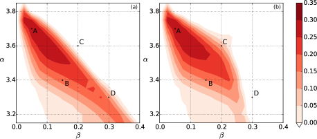
Figure 3: Many-body topological gap measured in units $J$ for eight bosons moving on a lattice $4\times 4$ two-site unit cells: (a) micromotion omitted, (b) micromotion included. The points labeled with the letters A, B, C, and D correspond to four typical behavioral patterns further analyzed in Fig. 4.

We start with the issue of stability of fractional states, and show in Fig. 3 the phase diagrams of eight bosons moving on a $4\times 4$ lattice. Here, the dependence of the topological many-body gap is plotted as a function of the scaled shaking strength $\alpha=Fd/\hbar\omega$ and scaled inverse frequency $\beta=J/\hbar\omega$ varying in the region of the largest band flatness detected in the single-particle simulations [see Fig. 2 (a)]. The left panel (a) refers to the case where micromotion is neglected, that is, the third-order term $\hat{H}_{F}^{(3)}$ is not included. In contrast, the right panel (b) presents the results obtained with micromotion taken into account. The colored regions correspond to the presence of a topological many-body gap, with the intensity encoding the size of the gap. The visible change of the shape indicates that micromotion has a significant impact on the stability of the fractional Chern insulator phase. The many-body gap closes for small $\beta$, since the single-particle gap closes for too large driving frequencies. However, it also closes for large values of $\beta$, that is, too slow shaking. To aid further analysis, we define four representative reference points A, B, C, and D seen in the phase diagrams of Fig. 3. At points A and B, micromotion seems to have no perceptible impact on the size of the topological band gap. At point C, the stability region has a shoulder where micromotion seems to enhance the fractional phase. Finally, at point D micromotion has a clearly detrimental effect. Here, the fractional Chern insulator phase is strongly suppressed.

The four reference locations on the phase diagram A, B, C, D exemplify four typical patterns observed in the interplay of micromotion and interactions and shown in Fig. 4. The four panels of this figure correspond to the four points and show the growth of the many-body gap as a function of the bare on-site repulsion strength $U$. The black lines connecting empty circles show the results obtained in the absence of micromotion effects, that is, when $\hat{H}_{F}^{(3)}$ is not taken into account. The red lines connecting data points marked by full circles correspond to the crudest approximation of the effects of micromotion on interactions: Here, only the on-site repulsion strength is reduced by including the correcting term (30a). As expected, this reduction leads to smaller many-body gaps as in all four panels the red line lies below the black one. As we have shown in the previous subsection, coupling between micromotion and interactions does not simply reduce the on-site repulsion energy but rather spreads it onto nearest-neighboring sites. Therefore, in our plot we include also the case when both these effects [i. e., both corrections (30a) and (30b)] are taken into account. The behavior of the many-body gap is now shown by the blue lines connecting cross-shaped markers. Evidently, the proper inclusion of micromotion-induced nearest-neighbor interactions generally has a significant stabilizing effect. Finally, the purple lines drawn over rhombus-shaped markers correspond the calculations that fully take the third-order correction into account. Thus, comparing the relative positions of purple and blue lines one may estimate the role of the density-assisted processes included at this last stage.

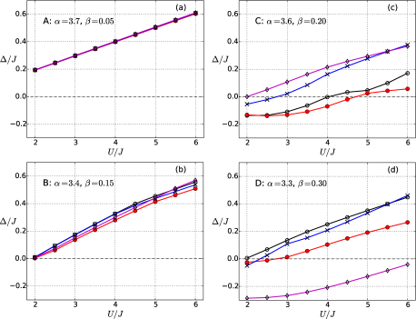
Figure 4: Many-body gap for eight bosons moving on a lattice $4\times 4$ at four typical parameter sets A, B, C, and D marked in Fig. 3. Black lines and empty circle markers: micromotion completely neglected, red lines with full circle markers: only reduction of on-site repulsion strength taken into account, blue lines with crosses: on-site repulsion spread onto neighboring sites, purple lines with rhombus-shaped markers: all third-order corrections included.

Proceeding to the analysis of the four typical patterns in panels (a)–(d) of Fig. 4, we begin with the reference point A in the top left corner of the shown phase diagram. Here, the fractional Chern insulator state is robust and the effect of third-order processes is minor due to the very small value of $\beta=0.05$ which corresponds to the high-frequency limit. Consequently, the four lines corresponding to the different levels of approximation nearly coincide in Fig. 4 (a). Moving along the line connecting point A to point B, one stays in the region characterized by large single-particle band flatness and robust fractional Chern insulator phase. However, the driving frequency is progressively lowered and the parameter $\beta$ reaches the value of $0.15$ at point B. Here, the four lines seen in Fig. 4 (b) start to diverge indicating that individual micromotion-related contributions have either a negative (reduction of on-site repulsion), positive (nearest-neighbor interactions) or varying (density-assisted hopping events) effect. However, the individual contributions largely cancel out and there is only a minor modification to the stability of the fractional phase.

Next, it is interesting to look at point C where the phase diagram indicates that micromotion-induced interactions may have a positive role on the topological many-body band gap. The results shown in Fig. 4 (c) show that this enhanced stability is mainly due to the positive impact of induced nearest-neighbor interactions. Finally, point D corresponds to relatively slow driving where micromotion has a very strong and evidently negative impact on the stability of the fractional Chern insulator. Our results shown in Fig. 4 (d) reveal that the destruction of the fractional phase is mainly due to rapidly growing negative contribution from the density-assisted hopping events.

V Summary and conclusions

To summarize, we have proposed a scheme for the realization of a Floquet topological band structure in a circularly shaken square lattice. Moreover, we have shown that in a driven system of interacting particles the presence of the real-space micromotion couples to the on-site inter-particle interactions and leads to the appearance of additional interaction terms in the effective Hamiltonian that allow for a physically transparent interpretation and classification. One part of the micromotion-induced contributions produces the effect of “smearing out” the on-site repulsion onto the nearest neighbors. The original (bare) on-site interaction energy is diminished and the missing portion is distributed over the links to nearest neighbors in a way that satisfies a strict constraint (33). Another part of the effects of micromotion lead to the appearance of density-assisted hopping terms. Applying our description to the bosonic fractional Chern insulator states at the filling factor $\nu=1/2$, we elucidate the role of the individual contributions on the stability of the fractional phase. It turns out that the fractional Chern insulators are largely destabilized by the density-assisted hopping events when their contribution becomes sufficiently large at lower driving frequencies. Note that also heating effects related to the creation of collective excitations (not captured by the high-frequency expansion) will become more and more important with decreasing driving frequency Eckardt and Anisimovas (2015). This suggests that the conditions for the preparation of a Floquet fractional Chern insulator are most favorable in the regime of rather large frequencies ($\hbar\omega\sim 10J$).

Appendix A Artificial gauge structures in driven lattices

A generic lattice model is defined by a set of lattice sites $i$ connected pairwise by a complementary set of connecting links. In our notation, $\langle ij\rangle$ denotes a directed link originating at site $j$ and running to site $i$. Thus, a purely kinetic Hamiltonian of a static (undriven) lattice reads

$$\hat{H}_{\text{st}}=-\sum_{\langle ij\rangle}J_{ij}\hat{a}^{{\dagger}}_{i}\hat{a}_{j}.$$ (34)

Here, $J_{ij}$ denotes the bare transition parameter, and $\hat{a}^{({\dagger})}_{i}$ are the standard annihilation (creation) operators defined on site $i$. Even though in standard situations $J_{ij}$ are real positive quantities, this model can be endowed with an artificial gauge structure by means of a time-periodic driving. In the present work, in addition to the lattice driving we also rely on the presence of staggered on-site potential shifts. Both effects are captured together by a potential-energy term

$$\hat{V}(t)=\sum_{i}v_{i}(t)\hat{a}^{{\dagger}}_{i}\hat{a}_{i},$$ (35)

written as a sum over lattice sites and featuring time- and coordinate-dependent on-site potentials of the form

$$v_{i}(t)=-\bm{F}(t)\cdot\bm{r}_{i}+s_{i}\hbar\omega.$$ (36)

Here, $\bm{r}_{i}$ is the position vector of the site $i$, $\bm{F}(t)$ is a time-periodic driving force oscillating with frequency $\omega$, and the static on-site energy shifts are characterized by integer factors $s_{i}$ times the energy quantum $\hbar\omega$. The potential term (35) can be eliminated from the Hamiltonian by means of a unitary transformation

$$\hat{U}(t)=\prod_{i}\hat{U}_{i}(t),\quad\hat{U}_{i}(t)=\exp\left[-\mathrm{i}\,\chi_{i}(t)\hat{a}^{{\dagger}}_{i}\hat{a}_{i}\right],$$ (37)

written as a product of independent operators acting on a single site and fulfilling the cancellation condition

$$\hat{U}^{{\dagger}}_{i}(t)v_{i}(t)\hat{a}^{{\dagger}}_{i}\hat{a}_{i}\hat{U}_{i}(t)-\mathrm{i}\hbar\hat{U}^{{\dagger}}_{i}(t)\partial_{t}\hat{U}_{i}(t)=0.$$ (38)

The phases $\chi_{i}(t)$ are obtained through a straightforward time integration

$$\begin{split}\chi_{i}(t)&=\frac{1}{\hbar}\int_{0}^{t}\!dt^{\prime}\,v_{i}(t^{\prime})+\gamma_{i}\\ &=-\frac{1}{\hbar}\int_{0}^{t}\!dt^{\prime}\,\bm{F}(t^{\prime})\cdot\bm{r}_{i}+s_{i}\omega t+\gamma_{i},\end{split}$$ (39)

with integration constants $\gamma_{i}$ reflecting the gauge freedom. The transformed Hamiltonian is purely kinetic

$$\hat{H}(t)=\hat{U}^{{\dagger}}(t)\hat{H}_{\text{st}}\hat{U}(t)=-\sum_{\langle ij\rangle}J_{ij}\,\mathrm{e}^{\mathrm{i}\theta_{ij}(t)}\hat{a}^{{\dagger}}_{i}\hat{a}_{j},$$ (40)

and features the Peierls phases

$$\begin{split}\theta_{ij}(t)&=\chi_{i}(t)-\chi_{j}(t)\\ &=-\frac{1}{\hbar}\int_{0}^{t}\!dt^{\prime}\,\bm{F}(t^{\prime})\cdot\bm{r}_{ij}+s_{ij}\,\omega t+\gamma_{ij}.\end{split}$$ (41)

Here, $\bm{r}_{ij}=\bm{r}_{i}-\bm{r}_{j}$, and likewise $s_{ij}=s_{i}-s_{j}$ and $\gamma_{ij}=\gamma_{i}-\gamma_{j}$.

In this work, we assume a circular driving protocol

$$\bm{F}(t)=-\hat{\bm{e}}_{x}F\cos(\omega t+\phi_{0})-\hat{\bm{e}}_{y}F\sin(\omega t+\phi_{0}),$$ (42)

equal hopping distances $|\bm{r}_{ij}|\equiv d$ and bare hopping parameters $J_{ij}\equiv J$, and define the polar angles $\varphi_{ij}$ measuring the direction of the vector $\bm{r}_{ij}$ with respect to the $x$ axis. Under these assumptions, the Peierls phases read

$$\theta_{ij}(t)=\alpha\sin\left(\omega t-\varphi_{ij}+\phi_{0}\right)+s_{ij}\,\omega t,$$ (43)

with the dimensionless shaking strength $\alpha=Fd/\hbar\omega$.

Appendix B High-frequency expansion of the effective Hamiltonian

The long-term dynamics generated by a time-periodic Hamiltonian is given by a time-independent effective Hamiltonian, and one’s ability to deliberately engineer its properties is known as the Floquet engineering. A standard approach to the construction of the effective Hamiltonian employs a series expansion in the powers of the inverse driving frequency. The successive terms in the series are conveniently expressed in terms of operator-valued Fourier components $\hat{H}_{s}$ of the driven Hamiltonian. Therefore we Fourier analyze the kinetic Hamiltonian

$$\hat{H}(t)=\sum_{s=-\infty}^{\infty}\hat{H}_{s}\,\mathrm{e}^{\mathrm{i}s\omega t}.$$ (44)

Specializing to static density-density interactions between particles we add them to the zeroth (static) Fourier component

$$\hat{H}_{0}\quad\to\quad\hat{H}_{0}+\hat{H}_{\text{int}}$$ (45)

The leading terms of the high-frequency expansion of the effective Hamiltonian Goldman and Dalibard (2014); Eckardt and Anisimovas (2015); Goldman et al. (2015); Bukov et al. (2015); Itin and Katsnelson (2015); Mikami et al.

$$\hat{H}_{F}=\hat{H}_{F}^{(1)}+\hat{H}_{F}^{(2)}+\hat{H}_{F}^{(3)}+\cdots$$ (46)

read

$$\hat{H}_{F}^{(1)} =\hat{H}_{0}+\hat{H}_{\text{int}},$$ (47a)

$$\hat{H}_{F}^{(2)} =\frac{1}{\hbar\omega}\sum_{s=1}^{\infty}\frac{1}{s}\big{[}\hat{H}_{s},\hat{H}_{-s}\big{]},$$ (47b)

$$\hat{H}_{F}^{(3)} =-\frac{1}{2(\hbar\omega)^{2}}\sum_{s=1}^{\infty}\frac{1}{s^{2}}\big{[}\big{[}\hat{H}_{0}+\hat{H}_{\text{int}},\hat{H}_{s}\big{]},\hat{H}_{-s}\big{]}+\mathrm{h.c.}.$$ (47c)

The commutator structure of the above expansion provides a clear physical interpretation of the successive contributions. Going beyond the high-frequency limit given by the time-averaged driven Hamiltonian $H_{F}^{(1)}$, in $\hat{H}_{F}^{(2)}$ one encounters combined hopping events that introduce next-neighbor transitions and help open a topological band gap in certain models, including also the example presented in this contribution. The physics is further enriched by the third order contribution $\hat{H}_{F}^{(3)}$, which can be separated into purely kinetic processes Mikami et al. given by $\big{[}\big{[}\hat{H}_{0},\hat{H}_{s}\big{]},\hat{H}_{-s}\big{]}$ and an interplay between the real-space micromotion and interactions encoded in $\big{[}\big{[}\hat{H}_{\text{int}},\hat{H}_{s}\big{]},\hat{H}_{-s}\big{]}$. In this work we focus on the latter effect and will not take the purely kinetic contribution into account. This is justified by two reasons. Firstly, the combined kinetic processes, being proportional to $\omega^{-2}$, are weak. On the other hand, the terms describing the interplay of micromotion and interactions are in addition scaled by the interaction strength, which in most situations relating to the formation of nontrivial phases must be large. Another reason pertains to the physical motivation – it is our primary goal to study the effects created by combining tunneling and interaction processes.

Appendix C Analysis of the auxiliary function $G$

To aid the analysis of the single-particle spectra, it is worthwhile to record some properties of the auxiliary function $G(\bm{k})$ defined by Eq. (10). Let us express the quasimomentum vector $\bm{k}$ in terms of its components along the elementary reciprocal lattice vectors

$$\bm{k}=k_{1}\bm{b}_{1}+k_{2}\bm{b}_{2},\quad\text{with}\quad\bm{a}_{i}\cdot\bm{b}_{j}=2\pi\delta_{ij},$$ (48)

so that $\bm{k}\cdot\bm{a}_{j}=2\pi k_{j}$, and we obtain for the absolute value of the $G$-function

$$\begin{split}\left|G_{s}(k_{1},k_{2})\right|^{2}&=4+4\cos\left(\frac{s\pi}{2}\right)\left(\cos 2\pi k_{1}+\cos 2\pi k_{2}\right)\\ &+4(-1)^{s}\cos 2\pi k_{1}\cos 2\pi k_{2}.\end{split}$$ (49)

Thus, for odd values of $s$ we have

$$\begin{split}\left|G_{s\text{ odd}}(k_{1},k_{2})\right|&=2\sqrt{1-\cos 2\pi k_{1}\cos 2\pi k_{2}}\end{split}$$ (50)

This function vanishes at two points within a Brillouin zone, namely, the center $\mathrm{D}_{1}:(k_{1}=0,k_{2}=0)$, and the corner $\mathrm{D}_{2}:\left(k_{1}=\tfrac{1}{2},k_{2}=\tfrac{1}{2}\right)$ of the square-shaped Brillouin zone. These are the two inequivalent Dirac points defined by the time-averaged driven Hamiltonian, hence the notation $\mathrm{D}_{1|2}$.

Turning now to the $G$-functions of even indices, we observe that they separate into two classes

$$\begin{split}\left|G_{s\text{ even}}(k_{1},k_{2})\right|^{2}&=4\left(1\pm\cos 2\pi k_{1}\right)\left(1\pm\cos 2\pi k_{2}\right),\end{split}$$ (51)

depending on the index $s$ being (upper sign $+$) or not being (lower sign $-$) a multiple of four; thus

$$|G_{4n}(k_{1},k_{2})|^{2} =16\,\cos^{2}\pi k_{1}\cos^{2}\pi k_{2},$$ (52a)

$$|G_{4n+2}(k_{1},k_{2})|^{2} =16\,\sin^{2}\pi k_{1}\sin^{2}\pi k_{2}.$$ (52b)

The values of these functions attained at the Dirac points are responsible for opening band gaps due to second-order hoppings. Thus we record (for an integer $n$) at $\mathrm{D}_{1}$:

$$\left|G_{4n}(0,0)\right|^{2}=16,\qquad\left|G_{4n+2}(0,0)\right|^{2}=0,$$ (53)

and at $\mathrm{D}_{2}$:

$$\left|G_{4n}\left(\tfrac{1}{2},\tfrac{1}{2}\right)\right|^{2}=0,\qquad\left|G_{4n+2}\left(\tfrac{1}{2},\tfrac{1}{2}\right)\right|^{2}=16.$$ (54)

When summed over the Fourier components, these numerical values lead to the band gap sizes given in Eq. (18a) and Eq. (18b) of the main text.