Near-field signal acquisition for smartglasses using two acoustic vector-sensors

Abstract

Smartglasses, in addition to their visual-output capabilities, often contain acoustic sensors for receiving the user’s voice. However, operation in noisy environments may lead to significant degradation of the received signal. To address this issue, we propose employing an acoustic sensor array which is mounted on the eyeglasses frames. The signals from the array are processed by an algorithm with the purpose of acquiring the desired near-field speech signal produced by the wearer while suppressing noise signals originating from the environment. The array is comprised of two acoustic vector-sensors which are located at the fore of the glasses’ temples. Each AVS consists of four collocated subsensors: one pressure sensor (with an omnidirectional response) and three particle-velocity sensors (with dipole responses) oriented in mutually orthogonal directions. The array configuration is designed to boost the input power of the desired signal, and to ensure that the characteristics of the noise at the different channels are sufficiently diverse (lending towards more effective noise suppression). Since changes in the array’s position correspond to the desired speaker’s movement, the relative source-receiver position remains unchanged; hence, the need to track fluctuations of the steering vector is avoided. Conversely, the spatial statistics of the noise are subject to rapid and abrupt changes due to sudden movement and rotation of the user’s head. Consequently, the algorithm must be capable of rapid adaptation toward such changes. We propose an algorithm which incorporates detection of the desired speech in the time-frequency domain, and employs this information to adaptively update estimates of the noise statistics. The speech detection plays a key role in ensuring the quality of the output signal. We conduct controlled measurements of the array in noisy scenarios. The proposed algorithm preforms favorably with respect to conventional algorithms.

1 Introduction

Recent years have witnessed an increased interest in wearable computers [1, 2]. These devices consist of miniature computers worn by users which can perform certain tasks; the devices may incorporate various sensors and feature networking capabilities. For example, a smartwatch may be used to display email messages, aid in navigation, and monitor the user’s heart rate (in addition to functioning as a timepiece).

One specific type of wearable computer which has garnered much attention is the smartglasses — a device which displays computer generated information supplementing the user’s visual field. A number of companies have been conducting research and development towards smartglasses intended for consumer usage [3] (e.g., Google Glass [4] and Microsoft HoloLens). In addition to their visual-output capabilities, smartglasses may incorporate acoustic sensors. These sensors are used for hands-free mobile telephony applications, and for applications using a voice-control interface to convey commands and information to the device.

The performance of both of these applications suffers when operating in a noisy environment: in telephony, noise degrades the quality of the speech signal transmitted to the other party; similarly, the accuracy of automatic speech recognition (ASR) systems is reduced when the desired speech is corrupted by noise. A review of one prominent smartglasses prototype delineated these two issues as requiring improvement [5].

To deal with these issues, we propose a system for the acquisition of the desired near-field speech in a noisy environment. The system is based on an acoustic array embedded in eyeglasses frames worn by the desired speaker. The multiple signals received by the array contain both desired speech as well as undesired components. These signals are processed by an adaptive beamforming algorithm to produce a single output signal with the aim of retaining the desired speech with little distortion while suppressing undesired components.

The scenario of a glasses mounted array presents some challenging features which are not encountered in typical speech processing. Glasses frames constitute a spatially compact platform, with little room to spread the sensors out. Typically, when sensors are closely spaced the statistical qualities of the noise at each sensor are highly correlated presenting difficulties in robust noise suppression [6]. Hence, special care must be taken in the design of the array.

The proposed array consists of two AVSs located, respectively, at the fore of the glasses’ right and left temples. In contrast to conventional sensors that measure only the pressure component of a sound field (which is a scalar quantity), an AVS measures both the pressure and particle-velocity components. An AVS consists of four subsensors with different spatial responses: one omnidirectional sensor (corresponding to pressure) and three orthogonally oriented dipole sensors (corresponding to the components of the particle-velocity vector). Hence, the array contains a total of eight channels (four from each AVS). Since each subsensor possesses a markedly different spatial response, the statistical properties of the noise at the different subsensors are diverse. Consequently, robust beamforming is possible in spite of the limited spatial aperture. Another advantage afforded by the use of AVSs is that the dipole sensors amplify near-field signals more so than conventional omnidirectional sensors. Due to these sensors, the desired speech signal (which is in the near-field due to the proximity to the sensors) undergoes a relative gain and is amplified with respect to the noise. The relative gain is explained and quantified in Sec. 2. The interested reader is referred to the Appendix for further information on AVSs.

The configuration in which the array is mounted on the speaker’s glasses differs from the typical scenario in which a microphone array is situated in the environment of the user. The glasses configuration possesses particular properties which lead to a number of benefits with respect to processing: (i) The close proximity of the desired source to the sensors leads to high signal-to-noise ratio (SNR) which is favorable. (ii) For similar reasons, the reverberation of the desired speech is negligible with respect to its direct component, rendering dereverberation a nonissue. (iii) Any change in the location of the desired source brings about a corresponding movement of the array which is mounted thereon. Consequently, the relative source-sensors configuration is essentially constant, precluding the need for tracking changes of the desired speaker’s position.

Conversely, the glasses-mounted configuration presents a specific challenge. The relative positions of the undesired acoustic sources with respect to the sensor array are liable to change rapidly. For instance, when the user rotates his/her head the relative position of the array to external sound sources undergoes significant and abrupt changes. This necessitates that the signal processing stage be capable of swift adaptation.

The proposed algorithm is based on minimum variance distortionless response (MVDR) beamforming which is designed to minimize the residual noise variance under the constraint of maintaining a distortionless desired signal. This type of beamforming was proposed by Capon [7] in the context of spatial spectrum analysis of seismic arrays. Frost [8] employed this idea in the field of speech processing using a time-domain representation of the signals. Later, Gannot et al. [9] recast the MVDR beamformer in the time-frequency domain. In the current work, we adopt the time-frequency formulation.

In the proposed algorithm, the noise covariance matrix is adaptively estimated on an ongoing basis from the received signals. Since the received signals contain both desired and undesired components, the covariance matrix obtained from a naive implementation would contain significant contributions of energy from the desired speech. This is detrimental to the performance of the processing. To prevent desired speech from contaminating the noise covariance estimation, a speech detection component is employed. Time-frequency bins which are deemed likely to contain desired speech are not used for estimating the noise covariance.

To further reduce noise, the output of the MVDR stage undergoes post-processing by a single-channel Wiener filter (SWF). It has been shown [10] that application of MVDR beamforming followed by a SWF is optimal in the sense of minimizing the mean square error (MSE) [since it is equivalent to the multichannel Wiener filter (MWF)].

The paper is structured as follows: Sec. 2 describes the motivation guiding our specific array design. In Sec. 3, we introduce the notation used to describe the scenario in which the array operates and then present the problem formulation. Sec. 4 presents the proposed algorithm and how its various component interrelate. Sec. 5 evaluates the performance of the proposed algorithm, and Sec. 6 concludes with a brief summary.

2 Motivation for array design

In this section, we discuss the considerations which lead to our choices for the placement of the sensors and the types of sensors used.

An AVS is located at the fore of each of the glasses’ temples (see Fig. 1). The reason for selecting this location is that there is a direct “line of sight” path from the speaker’s mouth to the sensors. For other locations on the frames, such as the temples’ rear sections or the areas above the lenses, the direct path is obstructed by human anatomy or the physical structure of the glasses. The areas underneath the lenses were also considered as they do have an unobstructed line to the mouth; however, embedding a microphone array at this locale was deemed to render the resulting frame structure too cumbersome.

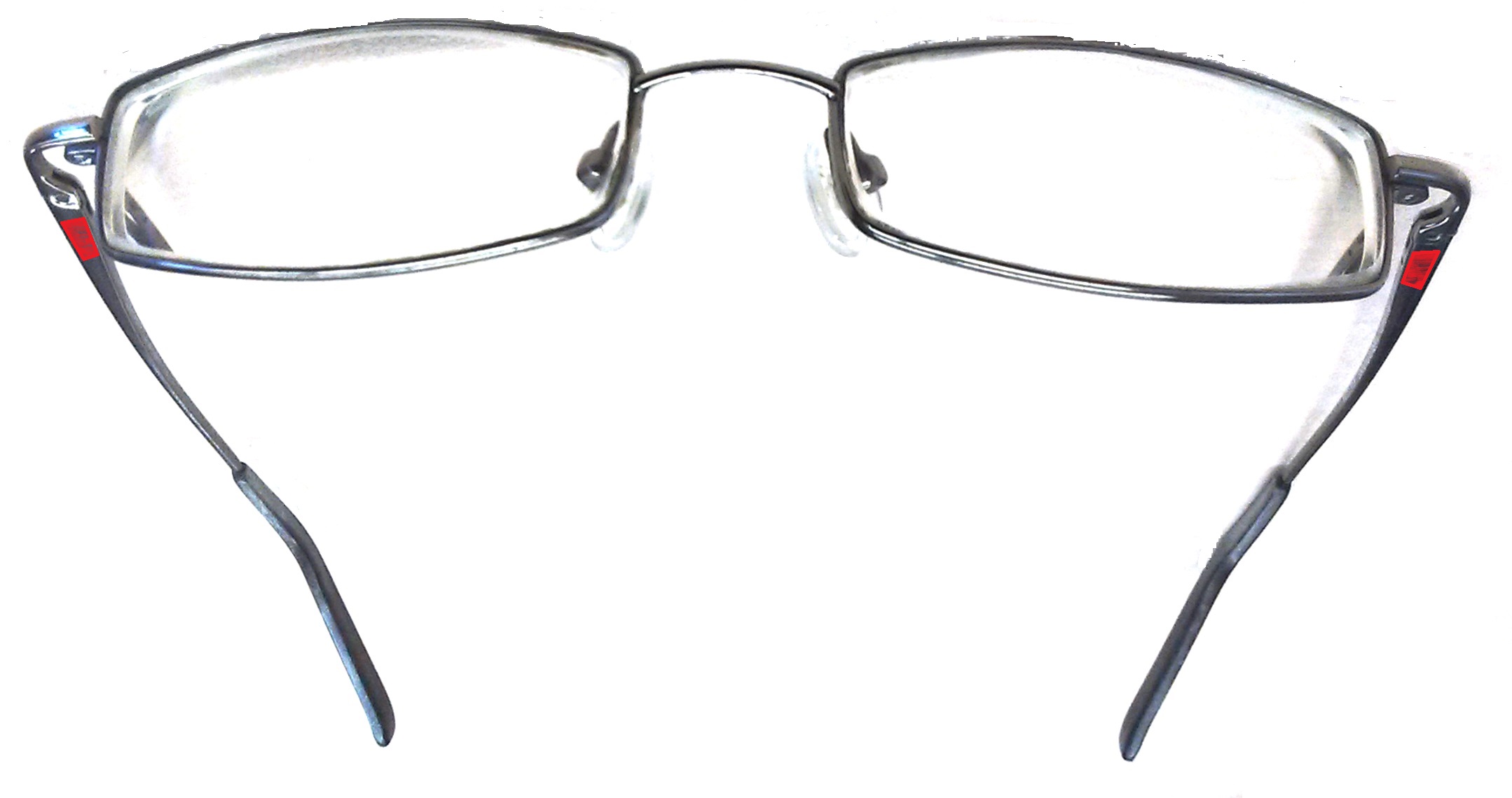
Figure 1: The proposed sensor locations are indicated in red.

Choosing an AVS based array, rather than using conventional sensors, leads to several advantages. Firstly, the inherent directional properties of an AVS lend to the distinction between the desired source and sound arriving from other directions. In contrast, a linear arrangement of conventional omnidirectional sensors along a temple of the glasses frame would exhibit a degree of directional ambiguity – it is known that the response of such linear arrays maintains a conical symmetry [11]. Secondly, an AVS preforms well with a compact spatial configuration, whereas conventional arrays suffer from low robustness when array elements are closely spaced [6]. Although this problem could be alleviated by allowing larger spacing between elements, this would necessitate placing sensors at the rear of the temple with no direct path to the source. Thirdly, the near-field frequency response of dipoles amplifies lower frequencies. This effect, which results from the near-field acoustic impedance, tends to increase the SNR since noise originating in the far-field does not undergo this amplification.

To illustrate this last point, we consider the sensors’ frequency responses to an ideal spherical wave[12]. The response of the monopole sensors is proportional to $\frac{1}{r}$, where $r$ is the distance from the wave’s origin (i.e., they have a flat frequency response). The response of the dipole elements is proportional to $\frac{1}{r}\left(1+\frac{c}{r}\frac{1}{j\omega}\right)$ where $c$ is the velocity of sound propagation and $\omega$ is the angular frequency. Consequently, the dipoles have a relative gain of $\left(1+\frac{c}{r}\frac{1}{j\omega}\right)$ over an omnidirectional sensor. This becomes particularly significant at short distances and lower frequencies where $r\ll\frac{c}{\omega}$. Stated differently, when the distance is significantly shorter than the wavelength, dipole sensors exhibit noticeable gain.

3 Notation and problem formulation

This section presents the scenario in which the array operates and the notation used to describe it. The problem formulation is then presented using this notation.

Let us denote the clean source signal as $s[n]$ and the $z_{1}[n]\ldots z_{P}[n]$ as $P$ interference signals. These signals propagate from their respective sources to the sensors and may also undergo reflections inducing reverberation. These processes are modeled as linear time invariant (LTI) systems represented by impulse-responses. Let $h_{m}[n]$ denote the response of the $m$-th sensor to an impulse produced by the desired source and $g_{m,p}[n]$ denote the impulse response from the $p$-th undesired source to the $m$-th sensor. Each of the $M=8$ sensors is also subject to ambient noise and internal sensor noise; these will be denoted $e_{m}[n]$. The resulting signal $x_{m}[n]$ received by the $m$-th sensor consists of all the above components and can be written as

$$x_{m}[n]=s[n]*h_{m}[n]+\left(\sum_{p=1}^{P}z_{p}[n]*g_{m,p}[n]\right)+e_{m}[n]\,.$$ (1)

Concatenating the respective elements into column-vectors, (1) can be reformulated as

$${\mathbf{x}}[n]=s[n]*{\mathbf{h}}[n]+\left(\sum_{p=1}^{P}z_{p}[n]*{\mathbf{g}}_{p}[n]\right)+{\mathbf{e}}[n]\,.$$ (2)

The impulse response ${\mathbf{h}}[n]$ can be decomposed into direct arrival and reverberation components ${\mathbf{h}}[n]={\mathbf{h}}_{{\mathrm{d}}}[n]+{\mathbf{h}}_{\mathrm{r}}[n]$. The received signals can be expressed as

$${\mathbf{x}}[n]=s[n]*{\mathbf{h}}_{\mathrm{d}}[n]+{\mathbf{v}}[n]\,,$$ (3)

where ${\mathbf{v}}[n]$ incorporates the undesired sound sources, ambient and sensor noise, and reverberation of the desired source. The vector ${\mathbf{v}}[n]$ and all its different subcomponents are referred to generically as noise in this paper. Since the sensors are mounted in close proximity to the mouth of the desired speaker, it can be assumed that the direct component is dominant with respect to reverberation (i.e., the direct-reverberation ratio (DRR) is high).

The received signals are transformed to the time-frequency domain via the short-time Fourier transform (STFT):

$${\mathbf{x}}[n]{\mapsto}{\mathbf{x}}(\ell,k)=\begin{bmatrix}X_{1}(\ell,k)\\ X_{2}(\ell,k)\\ \vdots\\ X_{M}(\ell,k)\end{bmatrix}\,,$$ (4)

where the subscript denotes the channel and the indexes $\ell$ and $k$ represent time and frequency indexes, respectively. A convolution in the time domain can be aptly approximated as multiplication in the STFT domain provided that the analysis window is sufficiently long vis-à-vis the length of the impulse response [9]. Since the direct component of the impulse response is highly localized in time, ${\mathbf{h}}_{\mathrm{d}}[n]$ satisfies this criterion. Consequently, (3) can be approximated in the STFT domain as

$${\mathbf{x}}(\ell,k)\,=\,{\mathbf{h}}_{\mathrm{d}}(k)s(\ell,k)+{\mathbf{v}}(\ell,k)\,.$$ (5)

Often the transfer function ${\mathbf{h}}_{\mathrm{d}}(k)$ is not available; therefore, it is convenient to use the relative transfer function (RTF) representation,

$${\mathbf{x}}(\ell,k)\,=\,{\widetilde{{\mathbf{h}}}_{\mathrm{d}}}(k){\widetilde{s}}(\ell,k)+{\mathbf{v}}(\ell,k)\,,$$ (6)

where ${\widetilde{s}}$ is typically the direct component of the clean source signal received at the first channel (or some linear combination of the different channels), and ${\widetilde{{\mathbf{h}}}_{\mathrm{d}}}(k)$ is the RTF of this signal with respect to the sensors. Expressed formally,

$${\widetilde{s}}(\ell,k)={\mathbf{c}}^{\mathrm{H}}(k){\mathbf{h}}_{\mathrm{d}}(k)s(\ell,k)\,,$$ (7)

where the vector ${\mathbf{c}}(k)$ determines the linear combination (e.g., ${\mathbf{c}}(k)=[1\,0\,\cdots\,0]^{{\mathrm{T}}}$ selects the first channel). The RTF vector, ${\widetilde{{\mathbf{h}}}_{\mathrm{d}}}(k)$, is related to the transfer function vector, ${\mathbf{h}}_{\mathrm{d}}(k)$, by

$${\widetilde{{\mathbf{h}}}_{\mathrm{d}}}(k)=\frac{{\mathbf{h}}_{\mathrm{d}}(k)}{{\mathbf{c}}^{\mathrm{H}}(k){\mathbf{h}}_{\mathrm{d}}(k)}\,.$$ (8)

We refer to ${\widetilde{s}}$ as the desired signal.

The signal processing system receives ${\mathbf{x}}[n]$ [or equivalently ${\mathbf{x}}(\ell,k)$] as an input and returns ${\widehat{s}}\;\![n]$, an estimate of the desired speech signal ${\widetilde{s}}[n]$, as the output. The estimate should effectively suppress noise and interference while maintaining low distortion and high intelligibility. The algorithm should have low latency to facilitate real time operation, and should be able to adapt rapidly to changes in the scenario.

4 Proposed algorithm

The various stages of the proposed algorithm are presented in this section. The signal processing employs beamforming to suppress undesired components. A speech detection method is used to determine which time-frequency bins are dominated by the desired speech and thus facilitate accurate estimation of the statistics used by the beamformer. The beamformer’s single-channel output undergoes post-processing to further reduce noise. Initial calibration procedures for the estimation of RTFs and sensor noise are also described.

4.1 Beamforming framework

A beamformer forms a linear combination of the input channels with the objective of enhancing the signal. This operation can be described as

$$y(\ell,k)={\mathbf{w}}^{\mathrm{H}}(\ell,k){\mathbf{x}}(\ell,k)\,,$$ (9)

where $y(\ell,k)$ is the beamformer output, and ${\mathbf{w}}(\ell,k)$ is the weight vector. This can be in turn presented as a combination of filtered desired and undesired components

$$y(\ell,k)={\mathbf{w}}^{\mathrm{H}}(\ell,k){\widetilde{{\mathbf{h}}}_{\mathrm{d}}}(k){\widetilde{s}}(\ell,k)+{\mathbf{w}}^{\mathrm{H}}(\ell,k){\mathbf{v}}(\ell,k)\,.$$ (10)

The power of the undesired component at the beamformer’s output is

$$E\{|{\mathbf{w}}^{\mathrm{H}}(\ell,k){\mathbf{v}}(\ell,k)|^{2}\}={\mathbf{w}}^{\mathrm{H}}(\ell,k){\mathbf{\Phi}}_{{\mathbf{v}}{\mathbf{v}}}(\ell,k){\mathbf{w}}(\ell,k)\,,$$ (11)

where ${\mathbf{\Phi}}_{{\mathbf{v}}{\mathbf{v}}}(\ell,k)=E\{{\mathbf{v}}(\ell,k){\mathbf{v}}^{\mathrm{H}}(\ell,k)\}$. The level of desired-signal distortion can be expressed as

$$|{\mathbf{w}}^{\mathrm{H}}(\ell,k){\widetilde{{\mathbf{h}}}_{\mathrm{d}}}(\ell,k)-1|^{2}\,.$$ (12)

There is a certain degree of discrepancy between the dual objectives of reducing noise (11) and reducing distortion (12). The MVDR beamformer minimizes noise under the constraint that no distortion is allowed. Formally,

$${\mathbf{w}}_{\mathrm{MVDR}}(\ell,k)=\operatornamewithlimits{argmin}_{{\mathbf{w}}(\ell,k)}\{{\mathbf{w}}^{\mathrm{H}}(\ell,k){\mathbf{\Phi}}_{{\mathbf{v}}{\mathbf{v}}}(\ell,k){\mathbf{w}}(\ell,k)\}$$

$$\textrm{ s.t.}\quad\quad{\mathbf{w}}^{\mathrm{H}}(\ell,k)^{\mathrm{H}}{\widetilde{{\mathbf{h}}}_{\mathrm{d}}}(k)=0\,.$$ (13)

The solution to (4.1) is

$${\mathbf{w}}_{\mathrm{MVDR}}(\ell,k)=\frac{{\mathbf{\Phi}}_{{\mathbf{v}}{\mathbf{v}}}^{-1}(\ell,k){\widetilde{{\mathbf{h}}}_{\mathrm{d}}}(k)}{{\widetilde{{\mathbf{h}}}_{\mathrm{d}}}^{\mathrm{H}}(k){\mathbf{\Phi}}_{{\mathbf{v}}{\mathbf{v}}}^{-1}(\ell,k){\widetilde{{\mathbf{h}}}_{\mathrm{d}}}(k)}\,.$$ (14)

In contrast to MVDR beamforming’s constrained minimization of noise, the MWF preforms unconstrained minimization of the MSE (i.e., distortion is allowed). This leads to improved noise suppression but introduces distortion. Formally, the MWF is defined as

$${\mathbf{w}}_{\mathrm{MWF}}(\ell,k)=\operatornamewithlimits{argmin}_{{\mathbf{w}}(\ell,k)}E\{|{\mathbf{w}}^{\mathrm{H}}(\ell,k){\mathbf{x}}(\ell,k)-{\widetilde{s}}(\ell,k)|^{2}\}\,.$$ (15)

It has been shown [13] that the MWF is equivalent to performing post-processing to the output of an MVDR beamformer with a single-channel Wiener filter (SWF):

$${\mathbf{w}}_{\mathrm{MWF}}(\ell,k)={\mathbf{w}}_{\mathrm{MVDR}}(\ell,k)\cdot W(\ell,k)\,.$$ (16)

An SWF, $W(\ell,k)$, is determined from the SNR at its input (in this case the output of a beamformer). The relationship is given by

$$W(\ell,k)=\frac{1}{1+\mathrm{SNR}^{-1}(\ell,k)}\,.$$ (17)

We adopt this two-stage perspective and split the processing into an MVDR stage followed by Weiner based post-processing.

For the MVDR stage, knowledge of the RTF ${\widetilde{{\mathbf{h}}}_{\mathrm{d}}}(k)$ and of the noise covariance ${\mathbf{\Phi}}_{{\mathbf{v}}{\mathbf{v}}}(\ell,k)$ are required to compute the beamformer weights of (14). The RTF ${\widetilde{{\mathbf{h}}}_{\mathrm{d}}}(k)$ can be assumed to remain constant since the positions of the sensors with respect to the mouth of the desired source are fixed. Therefore, ${\widetilde{{\mathbf{h}}}_{\mathrm{d}}}(k)$ can be estimated once during a calibration procedure and used during all subsequent operation. A framework for estimating the RTF is outlined in Sec. 4.5.2.

The noise covariance ${\mathbf{\Phi}}_{{\mathbf{v}}{\mathbf{v}}}(\ell,k)$ does not remain constant as it is influenced by changes in the user’s position as well as changes of the characteristics of the undesired sources. Therefore, ${\mathbf{\Phi}}_{{\mathbf{v}}{\mathbf{v}}}(\ell,k)$ must be estimated on a continual basis. The estimation of ${\mathbf{\Phi}}_{{\mathbf{v}}{\mathbf{v}}}(\ell,k)$ is described in Sec. 4.2.

The post-processing stage described in Sec. 4.4 incorporates a scheme for estimating the SNR of (17). Measures to limit the distortion associated with Wiener filtering are also employed.

4.2 Noise covariance estimation

Since the noise covariance matrix ${\mathbf{\Phi}}_{{\mathbf{v}}{\mathbf{v}}}(\ell,k)$ may be subject to rapid changes, it must be continually estimated from the signal ${\mathbf{x}}(\ell,k)$. This may be accomplished by performing, for each frequency band, a weighted time-average which ascribes greater significance to more recent time samples. As a further requirement, we wish to exclude bins which contain the desired speech component from the average, since their inclusion introduces bias to the estimate and is detrimental to the beamformer’s performance. We estimate the noise variance as

$${\widehat{\mathbf{\Phi}}}_{{\mathbf{v}}{\mathbf{v}}}(\ell,k)=\alpha(\ell,k) {\widehat{\mathbf{\Phi}}}_{{\mathbf{v}}{\mathbf{v}}}(\ell-1,k)$$ (18)

$$+\big{(}1-\alpha(\ell,k)\big{)}{\mathbf{x}}(\ell,k){\mathbf{x}}^{\mathrm{H}}(\ell,k)\,,$$

where $\alpha$ is the relative weight ascribed to the previous estimate and $1-\alpha$ is the relative weight of the current time instant. If desired speech is detected during a given bin, $\alpha$ is set to 1, effectively ignoring that bin. Otherwise, $\alpha$ is set to $\alpha_{0}\in(0,1)$. Formally,

$$\alpha(\ell,k)=\begin{cases}1,&\text{if desired speech is detected}\\ \alpha_{0},&\text{otherwise.}\end{cases}$$ (19)

The parameter $\alpha_{0}$ is a smoothing parameter which corresponds to a time-constant $\tau$ specifying the effective duration of the estimator’s memory. They are related by

$$\alpha_{0}=e^{\frac{-\tau F_{s}}{R}}\Leftrightarrow\tau=\frac{-R}{F_{s}\ln(\alpha_{0})}\,,$$ (20)

where $F_{s}$ is the sample rate, $R$ is the hop size (i.e., number of time samples between successive time frames), and $\tau$ is measured in seconds.

In certain scenarios, ${\widehat{\mathbf{\Phi}}}_{{\mathbf{v}}{\mathbf{v}}}(\ell,k)$ is ill-conditioned and (14) produces exceptionally large weight vectors [14]. To counter this phenomenon, we constrain the norm of ${\mathbf{w}}$ to a maximal value,

$${\mathbf{w}}_{\mathrm{reg}}(\ell,k)=\begin{cases}{\mathbf{w}}_{\mathrm{MVDR}}(\ell,k),&\text{if }\|{\mathbf{w}}_{\mathrm{MVDR}}(\ell,k)\|_{2}\leq\rho\\ \rho\frac{{\mathbf{w}}_{\mathrm{MVDR}(\ell,k)}}{\|{\mathbf{w}}_{\mathrm{MVDR}(\ell,k)}\|},&\text{otherwise.}\end{cases}$$ (21)

In (21), ${\mathbf{w}}_{\mathrm{reg}}$ represents the regularized weight vector and $\rho$ is the norm constraint.

4.3 Narrowband near-field speech detection

To determine whether the desired speech is present in a specific time-frequency bin, we propose the test statistic

$$T(\ell,k)=\frac{|{\mathbf{x}}^{\mathrm{H}}(\ell,k){\widetilde{{\mathbf{h}}}_{\mathrm{d}}}(k)|^{2}}{|{\mathbf{x}}(\ell,k)|^{2}|{\widetilde{{\mathbf{h}}}_{\mathrm{d}}}(k)|^{2}}\,.$$ (22)

Geometrically, $T$ corresponds to the square of the cosine of the angle between the two vectors ${\mathbf{x}}$ and ${\widetilde{{\mathbf{h}}}_{\mathrm{d}}}$. The highest value which $T$ may obtain is 1; this occurs when ${\mathbf{x}}$ is proportional to ${\widetilde{{\mathbf{h}}}_{\mathrm{d}}}$ corresponding to complete affinity between the received data ${\mathbf{x}}$ and the RTF vector ${\widetilde{{\mathbf{h}}}_{\mathrm{d}}}$. Speech detection is determined by comparison with a threshold value $\eta\,$: for $T(\ell,k)\geq\eta$, speech is detected; otherwise, speech is deemed absent. This criterion determines the value of $\alpha(\ell,k)$ in (19).

4.4 Post-processing

Post-filtering achieves further noise reduction at the expense of increased distortion. Weiner filtering (17) applies an SNR dependent attenuation (low SNRs incur higher levels of attenuation). However, the SNR is not known and needs to be estimated. We use a variation of Ephraim and Malah’s “decision-directed” approach [18], i.e.,

$$\begin{aligned} \gamma(\ell,k)&=\frac{|{\mathbf{w}}_{\mathrm{reg}}^{\mathrm{H}}(\ell,k){\mathbf{x}}(\ell,k)|^{2}}{{\mathbf{w}}_{\mathrm{reg}}^{\mathrm{H}}(\ell,k){\widehat{\mathbf{\Phi}}}_{{\mathbf{v}}{\mathbf{v}}}(\ell,k){\mathbf{w}}_{\mathrm{reg}}(\ell,k)}\\ \widehat{\mathrm{SNR}}(\ell,k)&=\beta|\widehat{W}(\ell-1,k)|^{2}\,\gamma(\ell-1,k)\\ &\quad\quad+(1-\beta)\max\{\gamma(\ell,k)-1,\,\mathrm{\mathrm{SNR_{min}}}\}\\ \widehat{W}(\ell,k)&=\max\left\{\frac{1}{1+\widehat{\mathrm{SNR}}^{-1}(\ell,k)},\,W_{\mathrm{min}}\right\}\,.\end{aligned}\$$ (23)

The parameters $\mathrm{SNR_{min}}$ and $W_{\mathrm{min}}$ set thresholds that, respectively, prevent the value of the estimated SNR of the current sample and the amplitude of the Wiener filter from being overly low. This limits the distortion levels and reduces the prevalence artifacts (such as musical tones). However, this comes at the expense of less powerful noise reduction.

Application of the post-processing stage to the output of the MVDR stage yields the estimated speech signal:

$$\widehat{s}(\ell,k)=\widehat{W}(\ell,k)\,{\mathbf{w}}^{\mathrm{H}}_{\mathrm{reg}}(\ell,k){\mathbf{x}}(\ell,k)\,.$$ (24)

The signal ${\widehat{s}}(\ell,k)$ which is in the time-frequency domain is then converted to the time domain to produce the system’s final output, ${\widehat{s}}\;\![n]$.

It should be noted that the above approach is fairly rudimentary. Other more elaborate post-processing techniques have been developed and tested (e.g., [19, 20, 21]). Our simpler choice of post-processing algorithm serves for the purpose of demonstrating a complete system of beamforming and post-processing applied to a smartglasses system. This concise algorithm could, in principal, be replaced with more sophisticated one. Furthermore, such algorithms could integrate information about speech activity contained in the test statistic $T(\ell,k)$.

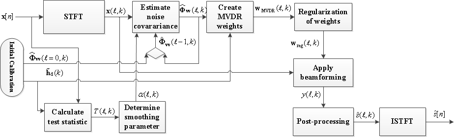
Figure 2: Block diagram schematic of the proposed algorithm.

4.5 Calibration procedures

We describe calibration procedures which are done prior to running the algorithm.

4.5.1 Sensor noise estimation

Offline, the covariance matrix of sensor noise is estimated. This is done by recording a segment in which which only sensor noise is present. Let the STFT of this signal be denoted ${\mathbf{a}}(\ell,k)$, and the number of time frames be denoted by ${L_{\mathrm{a}}}$. Since sensor noise is assumed stationary, the time-averaged covariance matrix, $\overline{{\mathbf{\Phi}}}_{{\mathbf{a}}{\mathbf{a}}}(k)=\frac{1}{{L_{\mathrm{a}}}}\sum_{\ell=1}^{L_{\mathrm{a}}}{\mathbf{a}}(\ell,k){\mathbf{a}}^{\mathrm{H}}(\ell,k)$, serves as an estimate of the covariance of sensor noise.

This is used in (18) as the initial condition value ${\widehat{\mathbf{\Phi}}}_{{\mathbf{v}}{\mathbf{v}}}(\ell-1,k)$. Specifically, we set ${\widehat{\mathbf{\Phi}}}_{{\mathbf{v}}{\mathbf{v}}}(\ell=0,k)=\overline{{\mathbf{\Phi}}}_{{\mathbf{a}}{\mathbf{a}}}(k)$. It should be noted that setting the initial value as zeros would be problematic since this leads to a series of singular matrices.

4.5.2 RTF estimation

System identification generally requires knowledge of a reference signal and the system’s output signals. Let ${\mathbf{b}}(\ell,k)$ represent the STFT of speech signals produced by a user wearing the glasses in a noise-free environment. For RTF estimation, the reference signal is ${\mathbf{c}}^{\mathrm{H}}(\ell,k){\mathbf{b}}(\ell,k)$ and the system’s outputs are ${\mathbf{b}}(\ell,k)$. An estimate of the RTF vector is given by

$$\widetilde{{\mathbf{h}}}_{\mathrm{est}}(k)=\frac{\sum_{\ell=1}^{L_{\mathrm{b}}}{\mathbf{b}}(\ell,k){\mathbf{b}}^{\mathrm{H}}(\ell,k){\mathbf{c}}(\ell,k)}{\sum_{\ell=1}^{L_{\mathrm{b}}}|{\mathbf{c}}^{\mathrm{H}}(\ell,k){\mathbf{b}}(\ell,k)|^{2}}\,,$$ (25)

where ${L_{\mathrm{b}}}$ denotes the number of time frames, and division is to be understood in an element-wise fashion.

Since, the desired RTF ${\widetilde{{\mathbf{h}}}_{\mathrm{d}}}(k)$ is comprised only of the direct component, the input and output signals would ideally need to be acquired in an anechoic environment. The availability of such a measuring environment is often not feasible, especially if these measurements are to be preformed by the end consumer. This being the case, reliance on (25) can be problematic, since reverberation is also incorporated into $\widetilde{{\mathbf{h}}}_{\mathrm{est}}(k)$. (We note that this information about reverberation in the training stage is not useful for the algorithm, since the during actual usage reverberation changes.)

To overcome the problem, we suggest a method based of (25) in which the estimation of ${\widetilde{{\mathbf{h}}}_{\mathrm{d}}}(k)$ may be conducted in a reverberant environment. We propose that RTF be estimated from measurements in which the speaker’s position shifts during the course of the measurement procedure. Alternatively, we may apply (25) to segments recorded at different positions, and average the resulting estimates of ${\widetilde{{\mathbf{h}}}_{\mathrm{d}}}(k)$. The rationale for this approach is that the reverberant components of the RTF change with the varying positions and therefore tend to cancel out. The direct component, on the other hand is not influenced by the desired speaker’s position.

4.6 Summary of algorithm

A block diagram depicting how the different components of the algorithm interrelate is presented in Fig. 2. The algorithm receives the multichannel input signal ${\mathbf{x}}[n]$ and produces a single-channel output ${\widehat{s}}\;\![n]$. Below, we describe the operations of the various blocks and refer the reader to the relevant formulas.

• The STFT and ISTFT blocks perform the short-time Fourier transform and inverse short-time Fourier transform, respectively. The main body of the algorithm operates in the time-frequency domain, and these conversion steps are required at the beginning and end of the process.

• The Initial calibration procedures estimate the RTF and the initial noise matrix (as described in Sec. 4.5).

• The Calculate test statistic block calculates $T(\ell,k)$ from (22).

• The Determine smoothing parameter block determines the value of $\alpha(\ell,k)$ according to (19). The criterion $T(\ell,k)\geq\eta$ signifies speech detection.

• The Estimate noise covariance block calculates (18).

• The Create MVDR weights block calculates (14).

• The Regularization of weights block calculates (21).

• The Apply beamforming block calculates (9), producing a regularized MVDR beamformer output.

• The post-processing block corresponds to Sec. 4.4.

5 Performance evaluation

This section describes experiments conducted to evaluate the proposed algorithm. The ensuing quantitative results are presented and compared to other algorithms. The reader is referred to the associated website [22] in order to listen to various audio signals.

5.1 Recording setup

First, we describe experiments which were conducted to evaluate the performance of the proposed algorithm. To perform the measurements, we used two Microflown USP probes [23]. Each of these probes consists of a pressure sensor and three particle-velocity sensors. The physical properties of particle-velocity correspond to a dipole directivity pattern.

The USP probes were fastened to the temples of eyeglasses which were placed on the face of a head and torso simulator (HATS) (Brüel Kjær 4128C). The HATS is a dummy which is designed to mimic the acoustic properties of a human being. For the sake of brevity, we refer to our HATS by the nickname ‘Cnut’. The distance from the center of Cnut’s mouth to the AVSs is approximately $10\frac{1}{2}$ cm. Fig. 3 shows a photograph of Cnut wearing the glasses array.

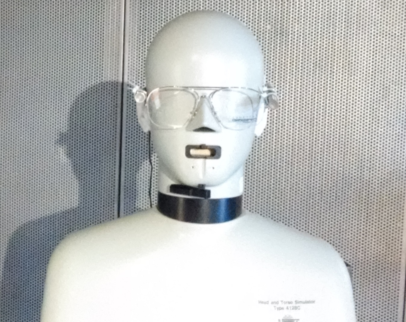
Figure 3: Photograph of Cnut, our head and torso simulator (HATS), eyeglasses array. The distance from the center of Cnut’s mouth to the AVSs is approximately $10\frac{1}{2}$ cm.

Recordings of several acoustic sources were preformed in a controlled acoustic room. These include the following five distinct voices:

1. A male voice, emitted from an internal loudspeaker located in Cnut’s mouth. This recording was repeated four separate times, with changes made to Cnut’s position or orientation between recordings. Three of the recordings were used for RTF estimation (as described in Sec. 4.5.2). The fourth recording was used to evaluate performance. All other sources used for evaluation (i.e., #2–#5) were recorded with Cnut in this fourth position and orientation.

2. A male voice emitted from an external static (i.e., non-moving) loudspeaker.

3. A female voice emitted from an external static loudspeaker.

4. A male voice emitted from an external static loudspeaker.

5. A male voice produced by one of the authors while walking in the acoustic room.

These five separate voices were each recorded independently. Sources #2, #3, and #4 were located respectively to at the front-right, front, and front-left of Cnut and were positioned at a distance of approximately 1 meter from it. Source 5 walked along different positions of a semicircular path in the vicinity of sources #1–#3. A rough schematic of the relative positions of the sources is given in Fig. 4.

The recordings were conducted in the acoustic room at the speech and acoustics lab at Bar-Ilan University. The room dimensions are approximately 6 m $\times$ 6 m $\times$ 2.3 m. During the recordings the reverberation level was medium-low.

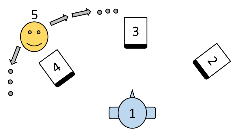
Figure 4: Schematic of the acoustic sources. #1: Cnut (the HATS); #2–#4: static loudspeakers; #5: moving human speaker. The distance between the HATS and loudspeakers is approximately 1 meter.

The use of independent recordings for each source allows for the creation of more complex scenarios by forming linear combinations of the basic recordings. These scenarios can be carefully controlled to examine the effects of different SNRs. Furthermore, since both the desired speech and undesired speech components are known, we can inspect how the algorithm effects each of these.

The recordings were resampled from 48 kHz to 16 kHz. Since the frequency-response of the USP sensors is not flat [23], we applied a set of digital filters to equalize the channels. These filters are also designed to counter nonumiformity of amplification across different channels and to remove low frequencies containing noise and high frequencies in the vicinity of 8 kHz (i.e., half the sampling rate of the resampled signals).

It should be noted that a sound wave with a frequency of 3.2 kHz has a wave length of approximately $10\frac{1}{2}$ cm, which corresponds to the distance between the center of Cnut’s mouth and the AVSs. For a typical speech signal, the bulk of the spectral energy in located beneath 3.4 kHz. Furthermore, the power spectrum of speech signals decays with increasing frequency [24]. Both of these characteristics are qualitatively evident in Fig. 5, which portrays the spectrogram of a segment of the signal emitted from Cnut’s mouth as recorded by the monopole sensors. (This signal serves as the clean signal for evaluation purposes in Sec. 5.3). Accordingly, the vast majority of the desired speech signal’s power corresponds to sub-wavelength propagation.

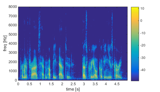
Figure 5: A spectrogram depicting a segment of the speech signal emitted from Cnut’s mouth as recorded by the monopole sensors.

5.2 Processing details

The calibration for sensor-noise was done with silent segments of the recordings and the RTF estimation was done with recordings of speaker #1 at different positions and orientations and no other speakers mixed in. The average of the two omnidirectional channels was used as the reference signal ${\widetilde{s}}(\ell,k)$ for estimating the RTF ${\widetilde{{\mathbf{h}}}_{\mathrm{d}}}(k)$. This corresponds to designating ${\mathbf{c}}$ of (7) as $\frac{1}{2}[1\,0\,0\,0\,1\,0\,0\,0]$.

The input signals upon which processing is preformed correspond to two scenarios. In the first scenario, three static speakers (#2–#4) were combined with equal levels of mean power. Afterwards, they were added to the desired source (#1) at different SNR levels. In the second scenario, source #5 was combined with source #1 at different SNR levels.

Each of the 8 channels is converted to the time-frequency domain by the STFT, and processed with the algorithm proposed in Sec. 4. Presently, the post-processing stage is omitted; it is evaluated separately in Sec. 5.5. An inverse STFT transform converts the output back into the time domain. The values for the parameters used are specified in Table 1.

Table 1: Parameter values used for testing proposed algorithm.

Parameter:	Value:
sampling frequency	$f_{\mathrm{s}}=16$ kHz
analysis window	512 sample Hamming window
hop size	$R=128$ samples
FFT size ()	1024 samples   (due to zero-padding)
synthesis window	512 sample Hamming window
smoothing parameter ()	$\alpha_{0}=0.98$ (corresponds to   $\tau\approx 0.396$ seconds)
norm constraint	$\rho=15$
speech detection  threshold	$\eta=0.9$

Several other algorithms are also examined as a basis for comparison. These algorithms include variations of MVDR and minimum power distortionless response (MPDR) beamforming and are described below:

1. Fixed-MVDR which uses a training segment in which only undesired components are present (i.e., prior to the onset of the desired speech) in order to calculate the sample covariance-matrix $\overline{{\mathbf{\Phi}}}_{{\mathbf{v}}{\mathbf{v}}}(k)$ which serves as an estimate of the noise covariance matrix. This matrix $\overline{{\mathbf{\Phi}}}_{{\mathbf{v}}{\mathbf{v}}}(k)$ is estimated only once and then used for the duration of the processing.

2. Fixed-MPDR which uses the sample-covariance matrix calculated from the segment to be processed. In MPDR beamforming [11], both desired and undesired signals contribute to the covariance matrix. The matrix, ${\mathbf{\Phi}}_{{\mathbf{v}}{\mathbf{v}}}$ is replaced by $\overline{{\mathbf{\Phi}}}_{{\mathbf{x}}{\mathbf{x}}}(k)$. In contrast to the fixed-MVDR algorithm, no separate training segment is used. Instead, the covariance matrix is estimated once from the entire segment to be processed, and used for the entire duration of the processing.

3. Adaptive-MPDR which uses a time-dependent estimate of the covariance matrix of the received signals, ${\widehat{\mathbf{\Phi}}}_{{\mathbf{x}}{\mathbf{x}}}(\ell,k)$. This is done by running the proposed algorithm with the threshold parameter set at $\eta=1$, effectively ensuring that $\alpha(\ell,k)=\alpha_{0}$ for all $\ell$ and $k$.

4. Oracle adaptation MVDR which uses a time-dependent estimate of the noise covariance matrix, ${\widehat{\mathbf{\Phi}}}_{{\mathbf{v}}{\mathbf{v}}}(\ell,k)$, based on the pure noise-component [i.e, ${\mathbf{x}}(\ell,k)$ of (18) is replaced by the undesired component $\mathbf{v}(\ell,k)$, and $\eta$ is set to 1]. The pure noise component is unobservable in practice, hence the denomination ‘oracle’; the algorithm is used for purposes of comparison.

5. The unprocessed signal (i.e., the average of the two omnidirectional sensors) is used for comparison with respect to the short-time objective intelligibility (STOI) measure. By definition, the noise reduction for the unprocessed signal is 0 dB and distortion is absent.

All algorithms use all eight channels of data. Furthermore, we apply the proposed algorithm and the oracle adaptation MVDR to the data from a reduced array containing only the two monopole channels. The obtained results provide an indication of the performance enhancement due to the additional six dipole channels present in the AVSs.

The feasibility of using these algorithms in practical settings varies. The fixed-MVDR algorithm presumes that segments containing only noise are available. The fixed-MPDR algorithm requires knowledge of the entire segment to be processed and hence cannot be used in real-time. Both the adaptive MPDR and the proposed algorithm are capable of operation in real-time. The oracle adaptation is not realizable since pure undesired components are unobservable in practice. Its function is purely for purposes of comparison.

5.3 Performance

In this subsection, we conduct an analysis of the proposed algorithm’s performance and compare it to the performance of other algorithms. Three measures are examined: (i) noise reduction (i.e., the amount by which the undesired component is attenuated); (ii) distortion (i.e., the amount by which the desired component of the output differs from its true value); (iii) the STOI measure [25].

Each of these three measures entails comparing components of the processed signal to some baseline reference. Since the signals at the eight different channels possess widely different characteristics, an arbitrary choice of a single channel to serve as the baseline, may produce misleading results. For instance, if a signal originates from the side of the array, the user’s head will shield some of the sensors. Selecting a signal from the right temple as opposed to the left temple to serve as the baseline may produce very different results. We elect to use the average of powers at the two omnidirectional sensors to define a signal’s power. In a similar fashion, the clean reference signal is taken as the average of the desired components received at the two omnidirectional sensors (which should be similar due to the geometrical symmetry of the corresponding direct paths). These definitions are stated formally below [(26)–(28)]. It should be stressed that this procedure relates to the evaluation but has no impact on the processing itself.

The procedure for testing an algorithm is as follows. An algorithm normally receives the data ${\mathbf{x}}[n]$, calculates the weights ${\mathbf{w}}_{\mathrm{alg}}(\ell,k)$, and applies them to produce the output ${\widehat{s}}_{\mathrm{alg}}[n]$. In our controlled experiments, the desired and noise components of ${\mathbf{x}}[n]$ are known. Hence, we can apply ${\mathbf{w}}(\ell,k)$ to the desired and noise components producing $d_{\mathrm{alg}}[n]$ and $v_{\mathrm{alg}}[n]$, respectively. Let us define ${\mathbf{w}}_{\mathrm{L}}(\ell,k)$ and ${\mathbf{w}}_{\mathrm{R}}(\ell,k)$ as weights which select only the left and right omnidirectional channel (i.e., the weight value for the selected channel is 1, and all other channel weights are 0 valued). In a similar manner, $d_{\mathrm{L}}[n]$, $d_{\mathrm{R}}[n]$, $v_{\mathrm{L}}[n]$, and $v_{\mathrm{R}}[n]$ are produced. The noise reduction is defined as

$$\text{noise reduction}=\frac{\frac{1}{2}\sum_{n}(v_{\mathrm{L}}^{2}[n]+v_{\mathrm{R}}^{2}[n])}{\sum_{n}v_{\mathrm{alg}}^{2}[n]}\,.$$ (26)

The distortion level is defined as

$$\text{distortion}=\frac{\sum_{n}\left(d_{\mathrm{alg}}[n]-\frac{1}{2}(d_{\mathrm{L}}[n]+d_{\mathrm{R}}[n])\right)^{2}}{\sum_{n}\left(\frac{1}{2}(d_{\mathrm{L}}[n]+d_{\mathrm{R}}[n])\right)^{2}}\,.$$ (27)

For calculating the STOI level, we compare the algorithm’s output ${\widehat{s}}_{\mathrm{alg}}[n]$ with

$$\mathrm{clean}[n]=\tfrac{1}{2}(d_{\mathrm{L}}[n]+d_{\mathrm{R}}[n])$$ (28)

functioning as the clean reference signal.

We proceed to analyze the results of the algorithms under test which utilize all eight channels (these are marked by solid lines). Afterwards, we return to the results which use only data from a reduced array (marked in a dotted line) and compare. Fig. 8 portrays the noise reduction results, Fig. 8 portrays the distortion results, and Fig. 8 portrays the STOI results. The SNRs examined range from -20 dB to 10 dB with increments of 5 dB; furthermore an SNR of 1000 dB is also examined (appearing at the right edge of the horizontal axis). This exceptionally high SNR is useful for checking robustness in extreme cases.

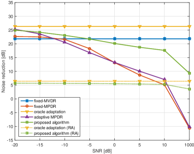
(a) 3 static interferers

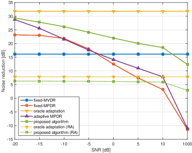
(b) 1 moving interferer

Figure 6: Noise reduction attained from processing with five different algorithms for varying SNR levels in two scenarios.

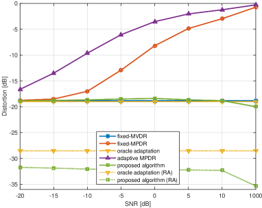
(a) 3 static interferers

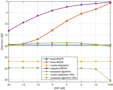
(b) 1 moving interferer

Figure 7: Distortion levels resulting from processing with five different algorithms for varying SNR levels in two scenarios.

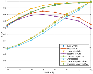
(a) 3 static interferers

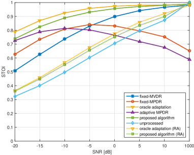
(b) 1 moving interferer

Figure 8: STOI levels resulting from processing with five different algorithms for varying SNR levels in two scenarios. (Note that for the static scenario (a), the fixed-MVDR and the proposed algorithm are nearly identical.)

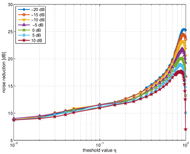
(a) 3 static interferers

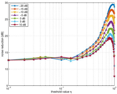
(b) 1 moving interferer

Figure 9: Noise reduction attained with the proposed algorithm using different values for the speech detection threshold ($\eta$) for a number of SNR levels.

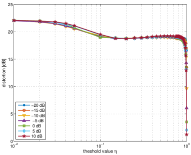
(a) 3 static interferers

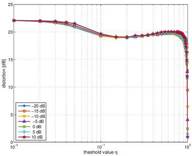
(b) 1 moving interferer

Figure 10: Distortion levels resulting from applying the proposed algorithm using different values for the speech detection threshold ($\eta$) for a number of SNR levels.

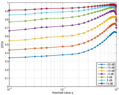
(a) 3 static interferers

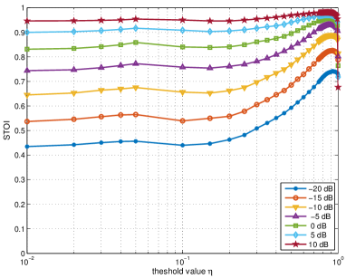
(b) 1 moving interferer

Figure 11: STOI levels attained with the proposed algorithm using different values for the speech detection threshold ($\eta$) for a number of SNR levels.

The results shown in the figures indicate that although both MPDR based algorithms perform reasonably well for low SNRs, there is a rapid degradation in performance as SNR increases. This can be explained by the contamination of the estimated covariance-matrix by desired speech, which is inherent in these methods. For very low SNRs the contamination is negligible, but at higher SNRs the contamination becomes significant. Due to this issue, the MPDR based algorithms cannot be regarded as viable.

With respect to distortion, the other algorithms (i.e., fixed-MVDR and proposed) score fairly well with levels between $-20$ dB and $-18$ dB. However, they differ with regards to noise reduction. For the static scenario, the fixed-MVDR attains a noise reduction of 21.8 dB. The proposed algorithm does slightly better at low SNRs ($-10$ dB and lower). At an SNR of $-5$ dB, the fixed-MVDR is slightly better and as the SNR increases the proposed algorithm’s noise reduction drops by several decibels (reaching 17.6 for an SNR of 10 dB). This is not decidedly troublesome since at high SNRs the issue of noise reduction is of lesser consequence.

For the case of moving interference, the proposed algorithm significantly outperforms fixed-MVDR. The fixed-MVDR algorithm reduces noise by 16.1 dB, whereas the proposed algorithm yields a reduction of 29.3 at $-20$ dB. As the SNR increases, the noise reduction gradually decreases but typically remains higher than the fixed-MVDR. For example, at SNRs of $-10$, 0, and 10 dB the respective noise reductions are 26.2, 22, and 18.5 dB. Due to the changing nature of the interference, the initial covariance estimate of the fixed-MVDR algorithm is deficient. In contrast, the proposed algorithm constantly adapts and consequently manages to effectively reduce noise. We note that the proposed algorithm is more successful in this dynamic case than in the case of 3 static interferers. This can be explained by the increased challenge of suppressing multiple sources.

The proposed algorithm significantly outperforms the fixed-MVDR algorithm in the scenario of a moving interferer with respect to STOI. Interestingly, in the static scenario the two algorithms have virtually indistinguishable STOI scores. This is despite the fact that there are differences in their noise reduction.

We now discuss the performance of the two algorithms tested with a reduced array (RA). These are labeled ‘oracle adaptation (RA)’ and ‘proposed algorithm (RA)’ in Figs 8, 8, and 8. The noise reduction attainable with the reduced array with the proposed algorithm is roughly 6 dB which is close to the limit set by oracle adaptation with a reduced array. Full use of all channels form the AVSs provided an improvement of approximately 15 to 25 dB. The performance with respect to STOI with a reduced array is only slightly better than the unprocessed signal. The distortion levels of the reduced array are in the vicinity of -30 dB which is an improvement over the full array with distortion of approximately -18 to -20 dB. This improvement is apparently due to the fact that the unprocessed signal was defined as the average of the two omnidirectional channels used by the reduced array. In any case, the full array preforms satisfactorily in terms of distortion and improvement is of negligible significance; utilization of all channels does provide significant improvements with respect to noise reduction and STOI.

5.4 Threshold parameter sensitivity

In this subsection, we examine the impact of the threshold parameter $\eta$ on the performance of the proposed algorithm. If $\eta$ is set too low, then too many bins are mistakenly labeled as containing desired speech. This may lead to poor noise estimation since fewer bins are used in the estimation process. Conversely, if $\eta$ is set too high, bins which do contain desired speech will not be detected as such which may lead to contamination of the noise estimation (as seen in the MPDR based algorithms). Presumably, a certain region of values in between these extremes will yield desirable results with respect to the conflicting goals.

We repeatedly executed the algorithm with $\eta$ taking on different values (the other parameters in Table 1 remain unchanged). This was done for SNRs ranging from $-20$ dB to 10 dB. The noise reduction results are plotted in Fig. 11, the distortion results in Fig. 11, and the STOI measure in Fig. 11. The STOI measures peak in the vicinity of $\eta=0.9$ and the curve is fairly flat indicating robustness. Similarly, $\eta=0.9$ is a fairly good choice with respect to noise reduction, although for low SNRs Fig. 11 indicates that a slight increase in $\eta$ is beneficial for low SNRs and conversely a slight decrease in $\eta$ is beneficial for high SNRs.

The distortion levels are somewhat better in the vicinity of $\eta$ = 0.6. However, since the distortion is minor, this slight improvement does not justify the accompanying degradation in noise and STOI which are of notable quantity.

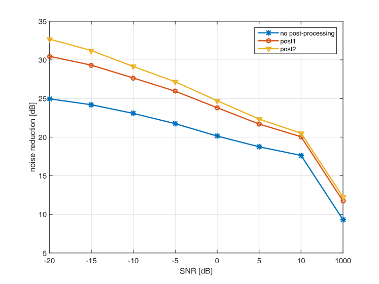
(a) Noise reduction

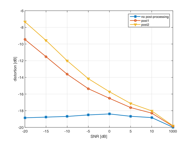
(b) Distortion

(c) STOI

Figure 12: Effects of post-processing on noise reduction, distortion, and STOI.

5.5 Post-processing results

In this subsection, we examine the effects of post-processing. Three parameters influence the post-processing: $\beta$, $\mathrm{SNR_{min}}$, and $W_{\mathrm{min}}$. Setting the latter two parameters at lower values corresponds to a more aggressive suppression of noise, whereas higher values correspond to a more conservative approach regarding signal distortion. To illustrate this trade-off, we test the two sets of parameters whose values are given in Table 2. These two sets are referred to as ‘post₁’ and ‘post₂’, respectively. In general, post-processing parameters are determined empirically; the designer tests which values yield results which are satisfactory for a particular application.

Table 2: Parameter values in post-processing.

Parameter:	$\bf{post_{1}}\textbf{:}$	$\bf{post_{2}}\textbf{:}$
$\beta$	0.9	0.9
$\mathrm{SNR_{min}}$	-10 dB	-24 dB
$W_{\mathrm{min}}$	-8 dB	-20 dB

Figure 12 portrays the effects of post-processing (using the three speaker scenario as a test case) on the performance. Post-processing reduces noise but increases distortion and adversely affects intelligibility as measured by STOI (this degradation is very minor for ‘post₁’ and more prominent in ‘post₂’). The parameters of ‘post₁’ are more conservative and the parameters of ‘post₂’ are more aggressive with respect to noise reduction. The former do not reduce as much noise, but have less distortion and only a minor degradation of STOI score. The latter reduce more noise at the expense of greater distortion and lower STOI. With the latter, audio artifacts have a stronger presence than the former. In general, the parameters may be adjusted to attain a desirable balance.

6 Conclusion

We proposed an array which consists of two AVSs mounted on an eyeglasses frame. This array configuration provides high input SNR and removes the need for tracking changes in the steering vector. An algorithm for suppressing undesired components was also proposed. This algorithm adapts to changes of the noise characteristics by continuously estimating the noise covariance matrix. A speech detection scheme is used to identify the presence of time-frequency bins containing desired speech and preventing them from corrupting the estimation of the noise covariance matrix. The speech detection plays a pivotal role in ensuring the quality of the output signal; in the absence of a speech detector, the higher levels of noise and distortion which are typical of MPDR processing are present. Experiments confirm that the proposed system performs well in both static and changing scenarios. The proposed system may be used to improve the quality of speech acquisition in smartglasses.

Appendix A Background on AVSs

A sound field can be described as a combination of two fields which are coupled: a pressure field and a particle-velocity field. The former is a scalar field and the latter is a vector field consisting of three Cartesian components.

Conventional sensors which are typically used in acoustic signal-processing measure the pressure field. Acoustic vectors sensors (AVSs) also measure the particle-velocity field, and thus provide more information: each sensor provides four components rather than one component.

An AVS consists of four collocated subsensors: one monopole and three orthogonally oriented dipoles. For a plane wave, each subsensor has a distinct directivity response. The response of a monopole element is

$$D_{\mathrm{mon}}=1\,,$$ (29)

and the response of a dipole element is

$$D_{\mathrm{dip}}={\mathbf{q}}^{T}{\mathbf{u}}\,,$$ (30)

where ${\mathbf{u}}$ is a unit-vector denoting the wave’s direction of arrival (DOA), and ${\mathbf{q}}$ is a unit-vector denoting the subsensor’s orientation. From the definition of scalar multiplication, it follows that $D_{\mathrm{dip}}$ corresponds to the cosine of the angle between the signal’s DOA and the subsensor’s orientation. The orientation of the three subsensors are ${\mathbf{q}}_{x}=[1\;0\;0]^{T}$, ${\mathbf{q}}_{y}=[0\;1\;0]^{T}$, and ${\mathbf{q}}_{z}=[0\;0\;1]^{T}$. The monopole response, which is independent of DOA, corresponds to the pressure field and the three dipole responses correspond to a scaled version of the Cartesian particle-velocity components. Fig. 13 portrays the magnitude of the four spatial responses.

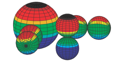
Figure 13: The magnitude of the directivity patterns of an AVS are plotted. They consist of a monopole and three mutually orthogonal dipoles.

For a spherical wave, the acoustical impedance is frequency-dependent. It can be shown that the dipole elements undergo a relative gain of $1+\frac{c}{r}\frac{1}{j\omega}$ over an omnidirectional sensor (as discussed in Sec. 2). This phenomenon is manifested particularly at lower frequencies for which the wavelength is significantly shorter than the source-receiver distance.

A standard omnidirectional microphone functions as a monopole element. Several approaches are available for constructing the dipole components of an AVS. One approach applies differential processing of closely-spaced omnidirectional sensors [26, 27, 28, 29]. An alternative approach employs acoustical sensors with inherent directional properties [30, 31]. Recently, an AVS based on microelectromechanical systems (MEMS) technology has been developed [23] and has become commercially available. The experiments discussed in Sec. 5 use such devices.

The different approaches mentioned produce approximations of the ideal responses. For instance, the subsensors can be placed close to each other but are not strictly collocated; spatial derivatives are estimated, etc. The approaches mentioned above differ with respect to attributes such as robustness, sensor noise, and cost. A discussion of these characteristics is beyond the scope of the current paper.

References

- [1] C. Randell, Wearable computing: a review, Tech. rep., Technical Report CSTR-06-004. University of Bristol (2005).
- [2] W. Barfield (Ed.), Fundamentals of wearable computers and augmented reality, CRC Press, 2016.
-
[3]
S. Cass, C. Q. Choi,
Google
Glass, HoloLens, and the real future of augmented reality, IEEE
Spectrum 52 (3) (2015) 18.
URL http://spectrum.ieee.org/consumer-electronics/audiovideo/google-glass-hololens-and-the-real-future-of-augmented-reality - [4] E. Ackerman, Google gets in your face: Google glass offers a slightly augmented version of reality, IEEE Spectrum 50 (1) (2013) 26–29.
-
[5]
D. Sung,
What’s
wrong with Google Glass?: the improvements the Big G needs to make before
Glass hits the masses (November 2014).
URL www.wareable.com/google-glass/google-glass-improvements-needed - [6] J. Bitzer, K. Simmer, Superdirective microphone arrays, in: M. Brandstein, D. Ward (Eds.), Microphone Arrays: Signal Processing Techniques and Applications, Springer-Verlag, 2001, Ch. 2, pp. 18–38.
- [7] J. Capon, High-resolution frequency-wavenumber spectrum analysis, Proceedings of the IEEE 57 (8) (1969) 1408–1418.
- [8] O. Frost, An algorithm for linearly constrained adaptive array processing, Proceedings of the IEEE 60 (8) (1972) 926–935.
- [9] S. Gannot, D. Burshtein, E. Weinstein, Signal enhancement using beamforming and nonstationarity with applications to speech, IEEE Transactions on Signal Processing 49 (8) (2001) 1614–1626.
- [10] K. U. Simmer, J. Bitzer, C. Marro, Post-filtering techniques, in: Microphone Arrays, Springer, 2001, pp. 39–60.
- [11] H. Van Trees, Detection, Estimation, and Modulation Theory, Vol. IV, Optimum Array Processing, Wiley, New York, USA, 2002.
- [12] A.D. Pierce, Acoustics: an introduction to its physical principles and applications, Acoustical Society of America, 1991.
- [13] A. Spriet, M. Moonen, J. Wouters, Spatially pre-processed speech distortion weighted multi-channel Wiener filtering for noise reduction, Signal Processing 84 (12) (2004) 2367–2387.
- [14] H. Cox, R. Zeskind, M. Owen, Robust adaptive beamforming, IEEE Trans. Acoust., Speech, Signal Process. 35 (10) (1987) 1365–1376.
- [15] E. Gilbert, S. Morgan, Optimum design of directive antenna arrays subject to random variations, Bell Syst. Tech. J 34 (1955) 637–663.
- [16] D. Levin, E. Habets, S. Gannot, et al., Robust beamforming using sensors with nonidentical directivity patterns, in: IEEE International Conference on Acoustics, Speech and Signal Processing (ICASSP), 2013, pp. 91–95.
- [17] K. Harmanci, J. Tabrikian, J. Krolik, Relationships between adaptive minimum variance beamforming and optimal source localization, IEEE Transactions on Signal Processing 48 (1) (2000) 1–12.
- [18] Y. Ephraim, D. Malah, Speech enhancement using a minimum-mean square error short-time spectral amplitude estimator, IEEE Transactions on Acoustics, Speech and Signal Processing 32 (6) (1984) 1109–1121.
- [19] I. A. McCowan, H. Bourlard, Microphone array post-filter based on noise field coherence, IEEE Transactions on Speech and Audio Processing 11 (6) (2003) 709–716.
- [20] S. Lefkimmiatis, D. Dimitriadis, P. Maragos, An optimum microphone array post-filter for speech applications, in: Interspeech – Int. Conf. on Spoken Lang. Proc., pp. 2142–2145.
- [21] S. Gannot, I. Cohen, Speech enhancement based on the general transfer function gsc and postfiltering, IEEE Trans. on Sp. and Au. Proc. 12 (6) (2004) 561–571.
-
[22]
Audio samples:
smartglasses.
URL www.eng.biu.ac.il/gannot/speech-enhancement/smart-glasses - [23] H.-E. de Bree, An overview of microflown technologies, Acta acustica united with Acustica 89 (1) (2003) 163–172.
- [24] U. Heute, Speech-transmission quality: aspects and assessment for wideband vs. narrowband signals, in: R. Martin, U. Heute, C. Antweiler (Eds.), Advances in digital speech transmission, John Wiley & Sons, 2008.
- [25] C. Taal, R. Hendriks, R. Heusdens, J. Jensen, An algorithm for intelligibility prediction of time-frequency weighted noisy speech, IEEE Trans. Audio, Speech, Lang. Process. 19 (7) (2011) 2125–2136.
- [26] H. F. Olson, Gradient microphones, Journal of the Acoustical Society of America 17 (3) (1946) 192–198.
- [27] G. Elko, A.-T. N. Pong, A simple adaptive first-order differential microphone, in: IEEE ASSP Workshop on Applications of Signal Processing to Audio and Acoustics, 1995, pp. 169 –172.
- [28] G. Elko, A.-T. N. Pong, A steerable and variable first-order differential microphone array, IEEE International Conference on Acoustics, Speech, and Signal Processing (ICASSP) 1 (1997) 223–226.
- [29] R. M. M. Derkx, K. Janse, Theoretical analysis of a first-order azimuth-steerable superdirective microphone array, IEEE Transactions on Audio, Speech, and Language Processing 17 (1) (2009) 150–162.
- [30] M. Shujau, C. H. Ritz, I. S. Burnett, Designing acoustic vector sensors for localisation of sound sources in air, in: 17th European Signal Processing Conference, 2009, pp. 849–853.
- [31] R. M. M. Derkx, First-order adaptive azimuthal null-steering for the suppression of two directional interferers, EURASIP Journal on Advances in Signal Processing 2010 (2010) 1.