Analytic queueing model for ambulance services
Abstract
We present predictive tools to calculate the number of ambulances needed according to demand of entrance calls and time of service. Our analysis discriminates between emergency and non-urgent calls. First, we consider the nonstationary regime where we apply previous results of first-passage time of one dimensional random walks. Then, we reconsider the stationary regime with a detailed discussion of the conditional probabilities and we discuss the key performance indicators.
1 Introduction
Emergency Medical Services (EMS) involve several operational decisions concerning optimizing the station location deployment for ambulances and the selection of the number of ambulances available in the fleet at different moments of the day or on different days in the week. Quantitative and predictive tools to assist the ambulance management are becoming increasingly important in the solution of economic and medical aspects of the problem [1]. Among these tools, modeling health care problems with queueing theory has gained in significance in the last sixty years [2].
Queueing theory has been used in the study of spatial and temporal distributions of demand of EMS in order of simulate the behavior of the system. Particularly, the ambulance location problem has been subject of considerable attention (See Refs. [3, 4, 5] and references therein) and has been applied to support decision making [6]. However, the problem of the number of ambulances required for service has received little mathematical attention beyond the prediction by the Little’s Law [7, 8]. The objective of this work is to derive useful quantities to predict the number of ambulances needed in real-time operation of EMS. This is a analytical work but with a didactic approach. We address here both modeling with clear mathematical derivations and their significance to operations research.
Our model is basically a call center [9] and can be described by exponential interarrival and service times, and servers: [10]. Thus, our queueing model is based on two average times: , the mean difference between call arrival times and , the mean service time of an individual ambulance. The service time involves the complete time lapse between the dispatch of the ambulance from the base and the its release for subsequent utilization. Thus, the service time sums up all the transport times of the ambulance plus the specific time for the medical attention at the scene. We are interested in the behavior of the system over a finite time interval, but long compared with and [11]. We focus on the nonstationary regime, where we apply the concept of the mean first-passage time (MFPT) [12], as well as in the stationary regime, where we are interested in the key performance quantities.
The paper is organized in three main sections. In Section 2 we describe the random walk model and the problem assumptions are emphasized. Section 3 focus on the calculation of the time to the next critical condition, that is when all ambulances are busy, whereas in Section 4 we discuss standard results of queueing theory with emphasis in the relevant performance indicators for the queue of clients and level of service of a home medical care service. Here, we also provide an alternative proof of the Little’s Law. The complementary mathematical details of Sections 3 and 4 are relegated to corresponding subsections in the appendix to enhance readability. Finally, in Section 5 we briefly summarize our main results.
2 The random walk model
Formally, we represent the system by the total number of ambulances in the service and by the number of received calls not served yet. is the state of occupation of the system. When , all the ambulances are in the base and there are not calls in queue. For , there are not waiting calls and ambulances are in course of action. That is, in transit from base to the call location, attending at patient location, or in transit to the hospital. In an equivalent way, we can say that there are patients simultaneously being served. When , the system is at the critical state. Even though there are not calls in waiting, all the servers have been assigned to calls and, in consequence, there are not any ambulance available to serve an eventual next incoming call. For , the system is saturated. All ambulances are occupied and there are calls waiting to be served in the queue.
At any time, the system can change its state between its nearest neighbors. Thus, the transition probability per unit time from the state to is denoted by , whereas the transition probability toward the lower occupation state is given by . In Figure 1, we sketch the possible transitions for the system.
The dynamics of the probability of finding the system at time in the state is ruled by the master equations of a random walk between nearest-neighbor sites with a reflecting boundary at the origin, that is a birth–death process [10],
| (1) |
We restrict our analysis to the case in which the times between calls and the service times are independent exponential random variables. The assumption that call arrival volume per unit of time is Poisson distributed is an standard choice in industry [13]. Thus, the time between calls is an exponential variable with rate or mean number of calls per unit time . On the other hand, the service time rate or mean number of attention per unit time and per ambulance results . Therefore, the transition probabilities are defined by [11]
| (2) |
In this manner, only depends on the state of the system. The average times and are all the experimental information needed to characterize the problem.
3 The critical emergency problem
The ambulance industry has the goal of provide care within 8 minutes for heart attack and cardiac arrest [14] and major trauma [15] (for critical considerations see Ref. [16]). Usually, the time lapse between picking the call up and the arrival of the ambulance at the scene is mainly consumed in transport. Thus, to achieve this goal is necessary to respond the calls immediately, without putting any EMS call in queue. Therefore, the most important aspect of emergency medical management is avoiding the saturation of the system. The prediction of the critical condition () is the particular interest for the quality of the medical service as much as the economic management of the service, given that the critical condition strongly depends on the number of ambulances simultaneously in service.
The mean time to the next critical condition is function of the initial state of the system, and can be calculated as the MFPT of a one dimensional random walk to site with a reflecting boundary at the opposite extreme (see Figure 1). For the critical problem, the initial condition is restricted to the values in the interval . MFPT is a dynamical variable that can not be computed in the steady state. Using known results in the literature [17], the mean time to the critical condition as function of the initial state of the system results
| (3) |
where the parameter . The mathematical details are given in Appendix 6.1.
Particularly, is the mean time between two critical conditions of the system, but without reaching saturation. Furthermore, as we want a quantity independent of the initial state, we average over . For this purpose, we define
| (4) |
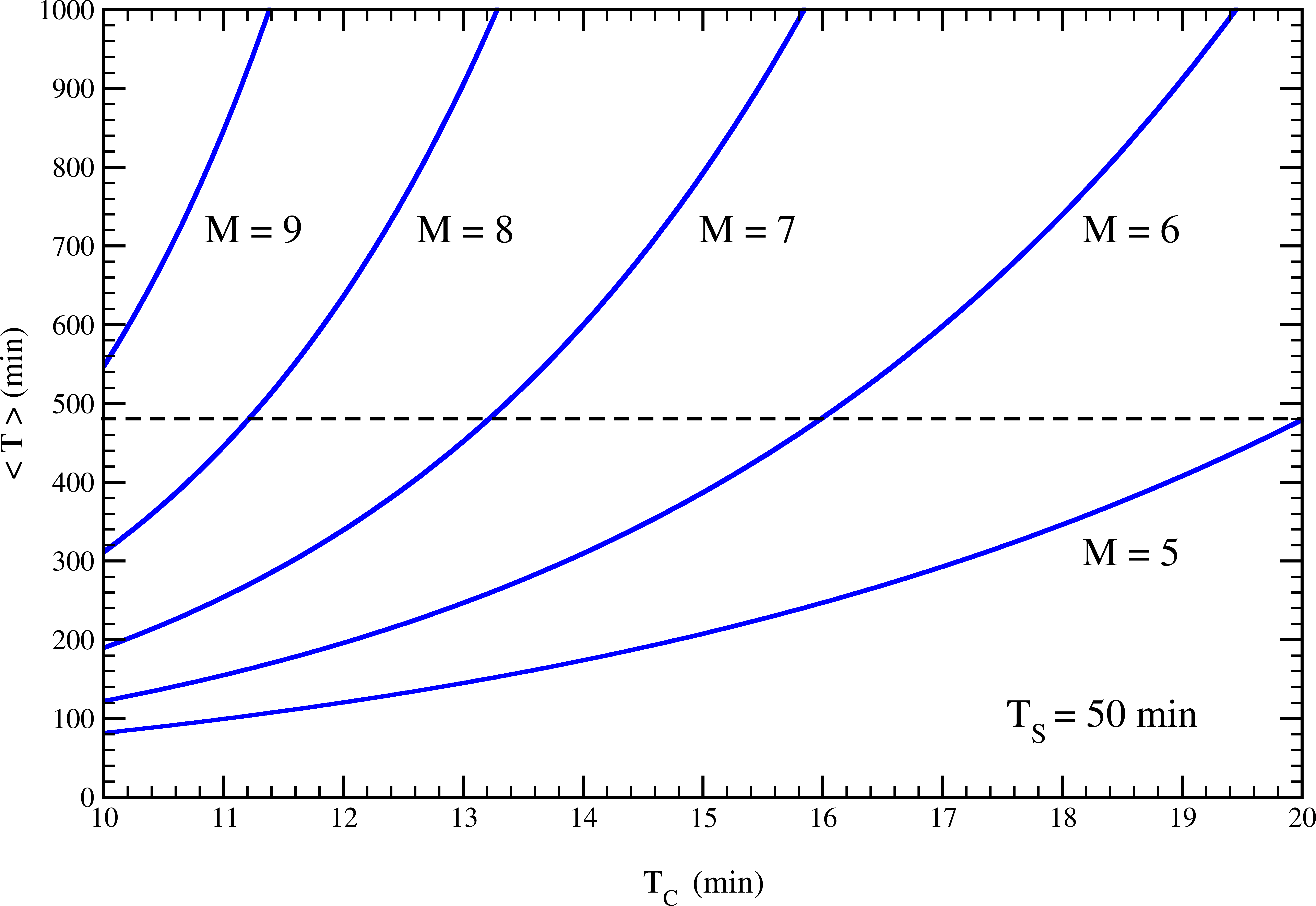
In this way, knowing the values of and , the expressions of Eq. (3) can be numerically evaluated in a very direct way. In Figure 2 we show the plots of , according to Eqs. (3) and (4), as function of the mean time between calls . We have sketched a characteristic situation where the mean service time is min and we considered the number of ambulances . The curves clearly show the non-linear behavior of .
Emergency medical care is an activity brought completely under protocol and in consequence the time of paramedic duties on scene have little variance. However, in a modern metropolis, transport time could consume an important part of the total service time and it have an specific hourly pattern. But, in practical situations, has small variations over the day in comparison with . The fluctuations of the rate of entrance calls, , have a defined pattern with marked differences during the day. Usually, the mean number of EMS calls per hour remains high during a time span of approximately eight hours between noon and 8:00 p.m. [13]. This distinct shape is similar for all days of the week.
Considering that is measured in the time interval of highest number of calls, the mean time to critical condition must be longer that this time span to ensure the service’s quality and avoiding saturation. For example, in Figure 2 we see that the system do not reach the critical condition within the interval of eight hours of high (horizontal dashed line) for min with six ambulances, and for min with seven ambulances.
In a similar way, to optimize the number of ambulances simultaneously in service, our analysis can be reproduced for any time interval of the day, for different days of the week, and at different locations of ambulance bases. Usually, the call rate , measured in a given interval during the day, is a linear function of the numbers of affiliates of the EMS but with seasonal fluctuations. This estimation gives us a reference for the average value of in the long term. In the short run, using the forecasting of the volume of call arrival [18, 13], our analysis allows us to estimate the diary and hourly demand of ambulances. Thus, we can easily design a simple and precise predictive tool for the fleet of ambulances required for a EMS by combining the use of estimation or forecasting of with our analysis of Figure 2, tailored for each particular case.
4 The non-urgent call problem
Most of the ambulance service providers, besides dealing with emergency calls, also bring medical home assistance for non-urgent calls. Usually, if a call is evaluated as non-urgent, the dispatcher derive it to another system to alleviate the use of emergency ambulances. In this case, contrary to the emergency management, non-urgent calls are allowed occasionally to be driven under saturation (). Thus, the length of the queue and the waiting time of the patients are the quantities of interest for the ongoing process. However, the system is driven in steady state only under a special condition.
4.1 Steady state
First, we define the dimensionless control parameter
| (5) |
which is also called traffic intensity in queueing theory [11]. The system has stationary state if and only if . Under this condition, the limit exists and according to the analysis of Appendix 6.2 is given by
| (6) |
where
| (7) |
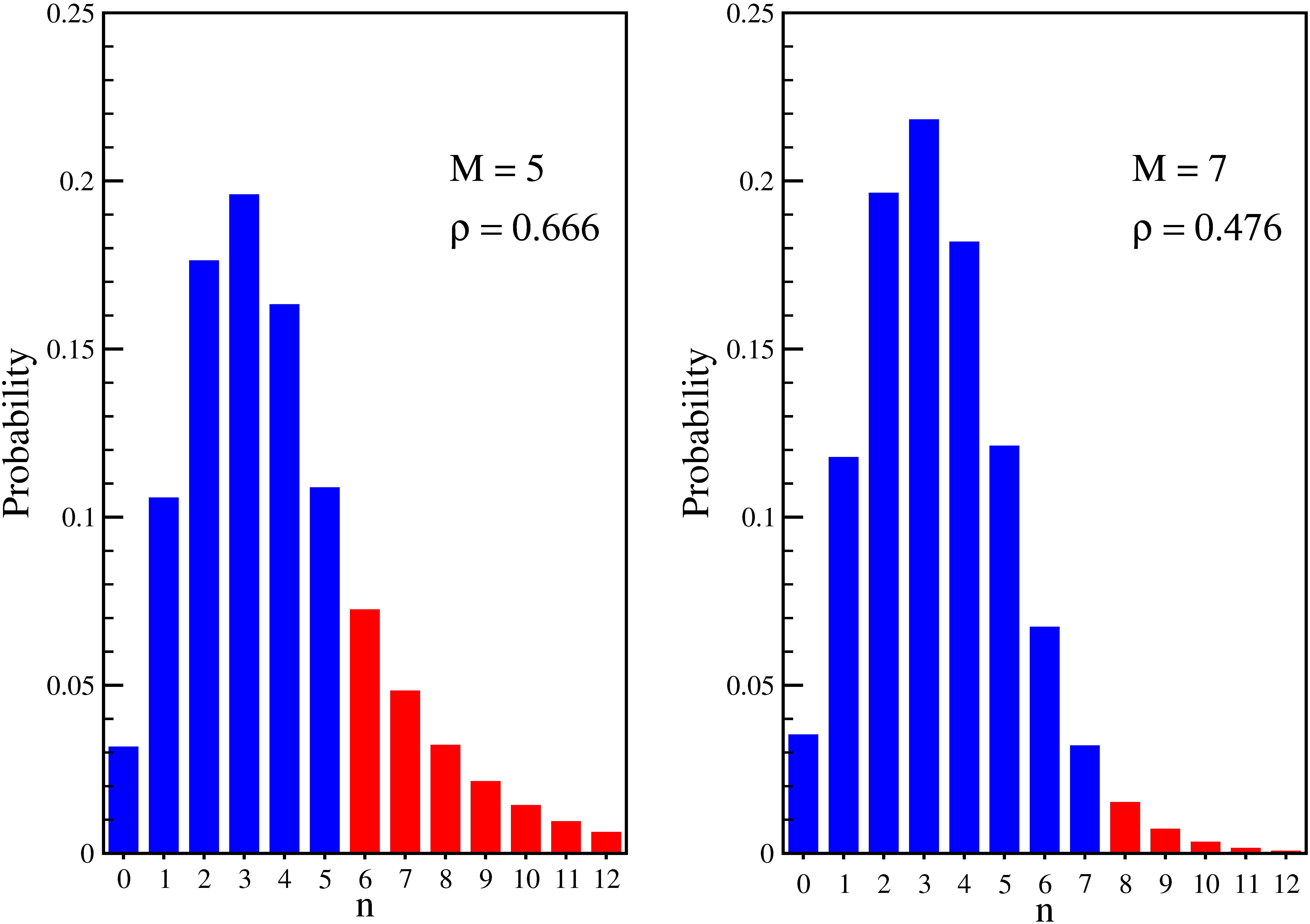
In Figure 3 we show plots for the probability distribution, according to Eqs. (6) and (7). Left panel corresponds to a fleet of five ambulances, whereas the right panel is for seven servers.
When the condition is not fulfilled, the probabilities are not defined. This situation corresponds to the collapse of the system when it is unable to deal with calls as fast as they arrive and the queue of waiting calls will develop without limit.
4.2 Queue length
If a call arrives when all servers are busy, it will be put in queue. The probability of full occupation of servers results
| (8) |
and under the condition , using Eq. (38), we obtain
| (9) |
The red tails in Figure 3 are the probabilities of full occupation for (left) and (right) ambulances, respectively.
To calculate the length of the genuine queue formed when the servers are busy, we need the conditional probability that the system is at state , given that all servers are occupied. From Eq. (6) (for ) and (9) we obtain
| (10) |
Setting , results that the conditional probability of having calls in the waiting row under full occupation is
| (11) |
This is the geometric distribution with parameter . Therefore, the average length of the genuine queue, , and its standard deviation, , result
| (12) |
Both quantities evidently diverge in the limit .
4.3 Quality of service
Now, we consider the arrival of a new call when the state of the system is , i.e., all servers are busy and there are calls in waiting. Under the queue discipline first-come, first-served, the time that the new patient will have to wait until an ambulance will be dispatched to his or her location, will be the sum of the waiting times of patients: The first in the row plus the time of any of the patients in service at the arrival time.
The probability distribution of the sum of exponential independent random variables with parameter is a Gamma distribution with parameters [19],
| (13) |
Thus, the conditional density of probability that a patient will be waiting a time given patients ahead in the row is given by Eq. (13) with and . We also know that the probability of having patients in the row is given by Eq. (11). Therefore, the probability density function of the waiting time in the row results
| (14) |
Summing up the series,
| (15) |
allows recast Eq. (14) as
| (16) |
Thus, we obtain an exponential distribution with parameter . In this manner, when all servers are busy, the mean waiting time of a patient in the row before being served is
| (17) |
The result is the expression of the well known Little’s Law [7, 8]. Our derivation is an alternative statistical approach in the stationary framework [20].
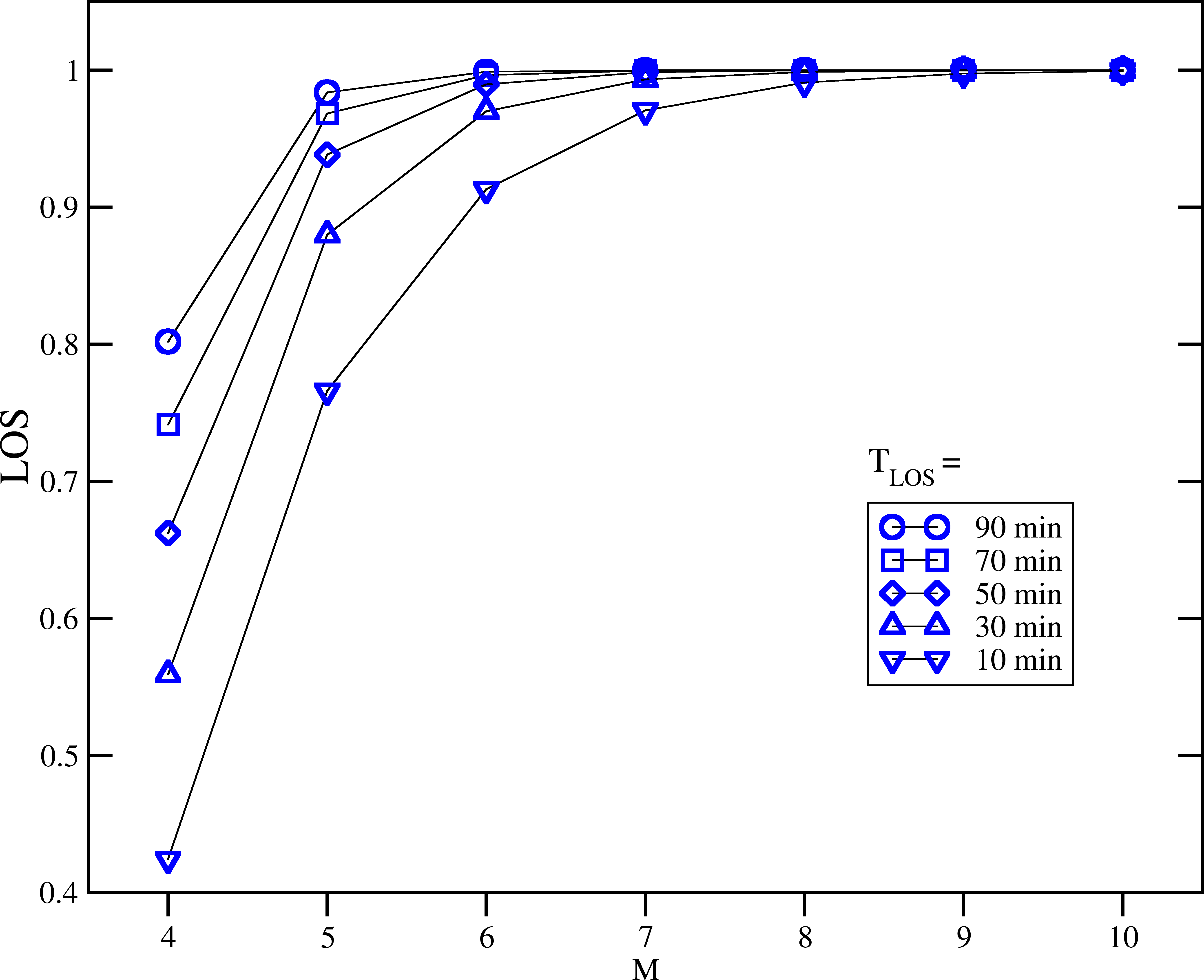
We define the level of service (LOS) as the fraction of patients served in a time less than a predefined threshold of quality . When a new call arrives, if there are idle servers, an ambulance is dispatched and there is not waiting time, but under full occupation, the quality threshold is fulfilled with probability
| (18) |
Thus, , and in our case we obtain,
| (19) |
where is given by Eq. (9). Then, if and only if which is the desired condition for management of emergency calls. In Figure 5, we illustrate the dependence of LOS in the number of ambulances.
4.4 Performance of servers
The probability that a given server is busy can be written as
| (20) |
where is given by Eq. (6) and is the conditional probability of a server busy given that the state of the system is . For and under the assumption that the assignment of calls to servers is at random if there is more than one idle, using simple combinatorial calculation, results
| (21) |
whereas, for , . Then,
| (22) |
Therefore, from Eqs. (6) and (9) results
| (23) |
In the stationary state, is the fraction of time that a given server remains busy. The dependence on of and is shown in Figure 6 for our example.
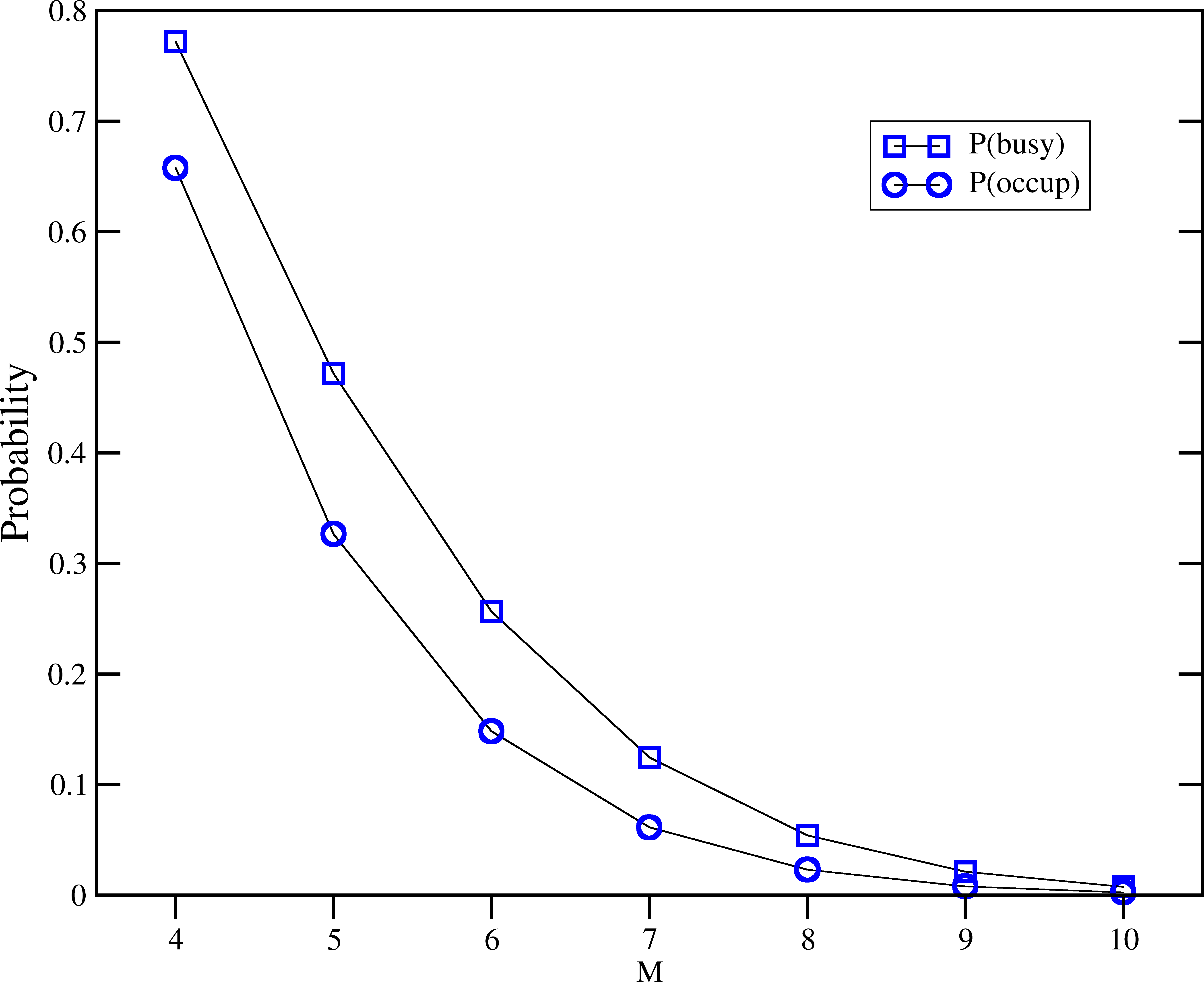
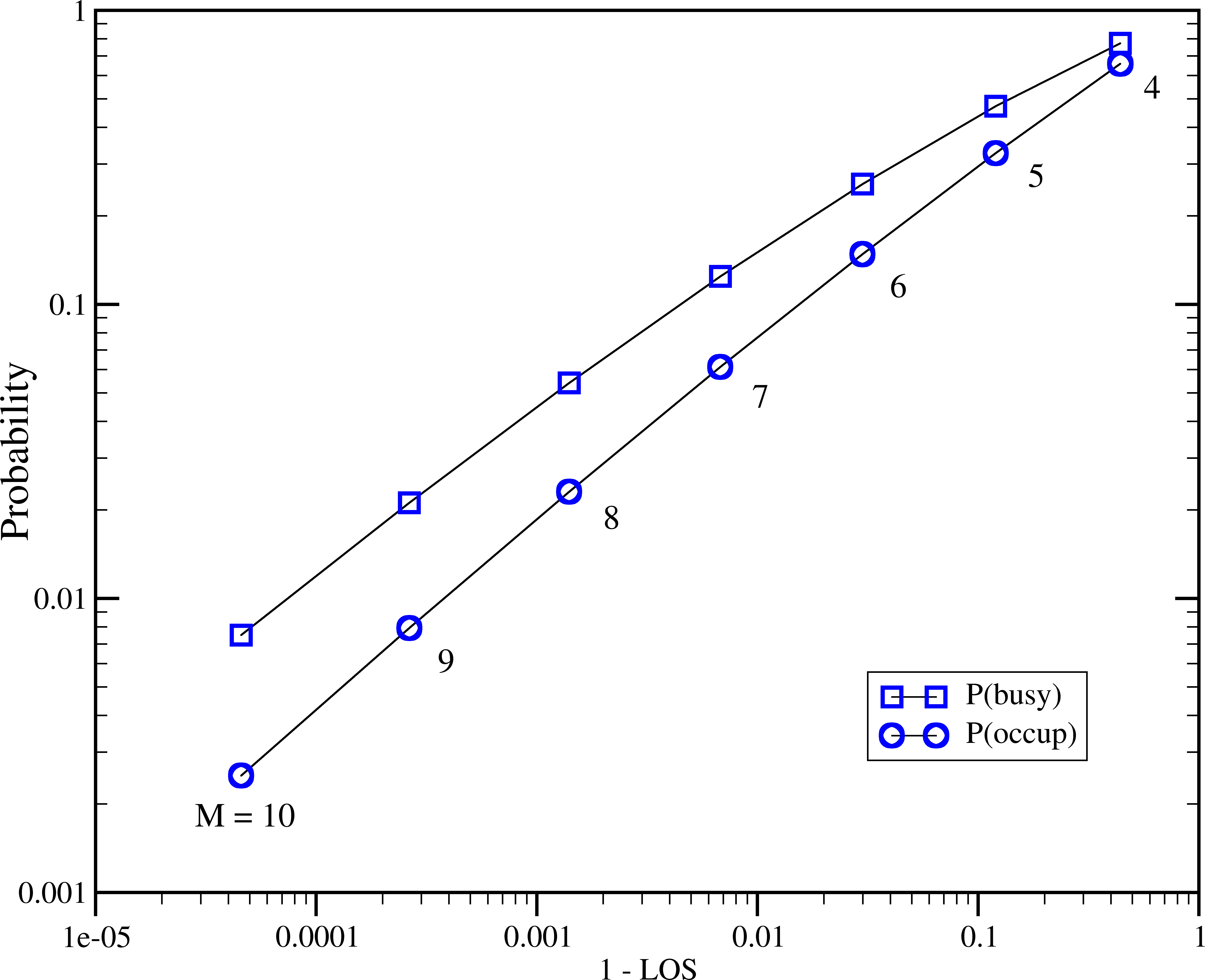
In this situation, from Figure 5 and 6, we can see that a fleet of six ambulances implies LOS greater than even though we choose small values of . However, a fleet of six ambulances remains completely occupied only of time and each server is busy only of time. To put in clear the trade-off between level of service and use of resources, we plot in Figure 7 the log-log plane of probability ( or ) and as function of . The graph is constructed for the fixed value min.
Alternatively, we can look at the mean number of medical attentions given by the system per unit of time,
| (24) |
From Eqs. (2) and (8), we obtain
| (25) |
In this way, if all servers are equivalents, the simple unit hour utilization, is given by . Last, but not least, if server’s cost per attention is , the cost per ambulance in the same unit of time results .
5 Concluding remarks
This work considers the mathematical problem of the number of ambulances needed in operation for a EMS according to the mean time between entrance calls and service times. We developed our analysis in the framework of the queueing theory for the nonstationary as well as for the stationary regime.
In Section 3 we presented a novel use of a previous result of MFPT for calculating the average time to the next critical condition of full occupation of servers. Our description allows to cope with the problem of the number of ambulances needed to avoid that condition. In Section 4 we rederived standard results of queueing theory for the stationary state emphasizing the use of conditional probabilities in the saturation regime when all servers are busy. We have paid special attention to the key performance indicators as queue length, level of service, and fraction of time of use of servers. Our analysis allows stress in simple mathematical terms the trade-off between quality of service and use of servers as function of fleet size.
6 Appendix: Mathematics of the random walk
6.1 MFPT
For asymmetric and site dependent transition probabilities, the analytical expressions for the MFPT of a random walk with a reflecting boundary condition, as shown in Figure 1, is given by [17],
| (26) |
In our model with servers, using Eq. (2) and the parameter defined in the text, we can recast the products in Eq. (26) as
| (27) |
Thus, we can also recast the sums in Eq. (26) as
| (28) |
and
| (29) |
Replacing the last two expressions in Eq. (26), we obtain Eq. (3) in Sec. 3 in the main text.
6.2 Steady state
Following [10], we can construct the steady state of the problem. From Eq. (1), the time independent solution must satisfy
| (30) |
Thus, from the first expression we immediately obtain
| (31) |
Substituting this result in the second equation () yields
| (32) |
and so on we can proof by induction that
| (33) |
From the normalization condition, , results
| (34) |
where
| (35) |
The existence of the steady state is determined by the convergence of the series in the Eq. (35).
For the model given by Eq. (2), the product in Eq. (35) can be written as,
| (36) |
Substituting Ec. (36) into Eq. (35) we obtain,
| (37) |
where is given by Eq. (5). The convergence of series in the last expression only occurs for . In this case,
| (38) |
and from Eqs. (33), (36), and (37), (38), we obtain the Eqs. (6) and (7) in the main text, respectively.
Acknowledgment
An early stage of this work was partially supported by Sistema de Urgencias del Rosafe SA, Córdoba, Argentina.
References
- [1] Jeffrey B. Goldberg. Operations research models for the deployment of emergency services vehicles. EMS Management Journal, 1(1):20–39, 2004.
- [2] C. Lakshmi and Appa Iyer Sivakumar. Application of queueing theory in health care: A literature review. Operations Research for Health Care, 2(1-2):25–39, 2013.
- [3] William K. Hall. Management science approaches to the determination of urban ambulance requirements. Socio-Econ. Plan. Sci., 5(5):491–499, 1971.
- [4] Geoffrey N. Berlin and Jon C. Liebman. Mathematical analysis of emergency ambulance location. Socio-Econ. Plan. Sci., 8(6):323–328, 1974.
- [5] Renata Algisi Takeda, João A. Widmer, and Reinaldo Morabito. Analysis of ambulance decentralization in an urban emergency medical service using the hypercube queueing model. Computers Operations Research, 34(3):727–741, 2007.
- [6] Marcos Singer and Patricio Donoso. Assessing an ambulance service with queuing theory. Computers Operations Research, 35(8):2549–2560, 2008.
- [7] John D. C. Little. A proof for the queuing formula: . Operations Research, 9(3):383–387, 1961.
- [8] John D. C. Little. Little’s law as viewed on its 50th anniversary. Operations Research, 59(3):536–549, 2011.
- [9] Ger Koole and Avishai Mandelbaum. Queueing models of call centers: An introduction. Annals of Operations Research, 113(1-4):41–59, 2002.
- [10] Wayne L. Winston. Operations Research: Applications and Algorithms. Duxbury Press, 4 ed. edition, 2003. Chap. 20.
- [11] David R. Cox and Walter L. Smith. Queues. Methuen, London, 1961.
- [12] Sidney Redner. A Guide to First-Passage Processes. Cambridge University Press, Cambridge, U.K., 2001.
- [13] David S. Matteson, Mathew W. McLean, Dawn B. Woodard, and Shane G. Henderson. Forecasting emergency medical service call arrival rates. Ann. Appl. Stat., 5(2B):1379–1406, 2011.
- [14] M.S. Eisenberg, L. Bergner, and A. Hallstrom. Cardiac resuscitation in the community: Importance of rapid provision and implications for program planning. JAMA: The Journal of the American Medical Association, 241(18):1905–1907, 1979.
- [15] Stan Feero, Jerris R. Hedges, Erik Simmons, and Lisa Irwin. Does out-of-hospital EMS time affect trauma survival? The American Journal of Emergency Medicine, 13(2):133–135, 1995.
- [16] Peter T Pons and Vincent J Markovchick. Eight minutes or less: does the ambulance response time guideline impact trauma patient outcome? The Journal of Emergency Medicine, 23(1):43–48, 2002.
- [17] Pedro A. Pury and Manuel O. Cáceres. Mean first-passage and residence times of random walks on asymmetric disordered chains. Journal of Physics A: Mathematical and General, 36(11):2695–2706, 2003.
- [18] Hubert Setzler, Cem Saydam, and Sungjune Park. EMS call volume predictions: A comparative study. Computers Operations Research, 36(6):1843–1851, 2009.
- [19] Sheldon M. Ross. Simulation. Elsevier Academic Press, 4 ed. edition, 2006. Pag. 31.
- [20] Song-Hee Kim and Ward Whitt. Statistical analysis with little’s law. Operations Research, 61(4):1030–1045, 2013.