Interactive Storytelling over Document Collections

Abstract

Storytelling algorithms aim to ‘connect the dots’ between disparate documents by linking starting and ending documents through a series of intermediate documents. Existing storytelling algorithms are based on notions of coherence and connectivity, and thus the primary way by which users can steer the story construction is via design of suitable similarity functions. We present an alternative approach to storytelling wherein the user can interactively and iteratively provide ‘must use’ constraints to preferentially support the construction of some stories over others. The three innovations in our approach are distance measures based on (inferred) topic distributions, the use of constraints to define sets of linear inequalities over paths, and the introduction of slack and surplus variables to condition the topic distribution to preferentially emphasize desired terms over others. We describe experimental results to illustrate the effectiveness of our interactive storytelling approach over multiple text datasets.

1 Introduction

Faced with a constant deluge of unstructured (text) data and an ever increasing sophistication of our information needs, a significant research front has opened up in the space of what has been referred to as information cartography [31]. The basic objective of this space is to pictorially help users make sense of information through inference of visual constructs such as stories [13, 17, 27, 28], threads [9, 10, 23], and maps [30, 29]. By supporting interactions over such constructs, information cartography systems aim to go beyond traditional information retrieval systems in supporting users’ information exploration needs.

Arguably the key concept underlying such cartography is the notion of storytelling, which aims to ‘connect the dots’ between disparate documents by linking starting and ending documents through a series of intermediate documents. There are two broad classes of storytelling algorithms, motivated by their different lineages. Algorithms focused on news articles [27, 28] aim for coherence of stories wherein every document in the story shares an underlying common theme. Algorithms focused in domains such as intelligence analysis [12] and bioinformatics [14] must often work with sparse information wherein a common theme is typically absent or at best tenuous. Such algorithms must leverage weak links to bridge diverse clusters of documents, and thus emphasize the construction and traversal of similarity networks. Irrespective of the motivations behind storytelling, all such algorithms provide limited abilities for the user to steer the story construction process. There is typically no mechanism to interactively steer the story construction toward desired story lines and avoid specific aspects that are not of interest.

In this paper, we present an alternative approach to storytelling wherein the user can interactively provide ‘must use’ constraints to preferentially support the construction of some stories over others. At each stage of our approach, the user can inspect the given story and the overall document collection, and express preferences to adjust the storyline, either in part or in overall. Such feedback is then incorporated into the story construction iteratively.

Our key contributions are:

1. Our interactive storytelling approach can be viewed as a form of ‘visual to parametric interaction’ (V2PI [18]) wherein users’ natural interactions with documents in a workspace is translated into parameter-level interactions in terms of the underlying machine learning models (here, topic models). In particular, we demonstrate how high-level user feedback at the level of paths is translated down to redefine topic distributions.

2. The underlying mathematical framework for interactive storytelling is a novel combination of hitherto uncombined components: distance measures based on (inferred) topic distributions, the use of constraints to define sets of linear inequalities over paths, and the introduction of slack and surplus variables to condition the topic distribution to preferentially emphasize desired terms over others. The proposed framework thus brings together notions from heuristic search, linear systems of inequalities, and topic models.

3. We illustrate how just a modicum of user feedback can be fruitfully employed to redefine topic distributions and at the same time severely curtail the search process in navigating large document collections. Through experimental studies, we demonstrate the effectiveness of our interactive storytelling approach over multiple text datasets.

2 Motivating Example

We present an illustrative example of how a storytelling algorithm can be steered toward desired lines of analysis based on user input. For our purposes, assume a vanilla storytelling algorithm (akin to [17, 15]) based on heuristic search to prioritize the exploration of adjacent documents in order to reach a desired destination document. Adjacency here can be assessed in many ways. One approach is to use local representations such as a tf-idf representation and define similarity measures (e.g., Jaccard coefficient) over such local representations. A second approach is to utilize the normalized topic distribution generated using, e.g., LDA [5], to induce a distance between every pair of documents.

Let us construct a toy corpus of $50$ documents wherein the terms are drawn from $9$ predefined themes and some random noise terms. Each theme is assumed to be represented by a collection of $4$ terms. An example of a theme is:
Theme 1: nation, terror, avert, orange
Each document is generated by a single theme or by mixing two themes. In addition to the terms sampled from the themes, each document is assumed to also contain $2$ noise terms. (The noise terms are document-specific meaning two documents do not share the same terms.) Thus, we obtain $4$ terms for each of the $9$ themes and $2$ noise terms for each of the $50$ documents, so that the total number of terms is $9\times 4+50\times 2=136$. A pair of documents has an edge between them if they have at least one common term. (Since noise terms are not common between the documents, they are not responsible for edge formation.) We use the notation $d_{n}(p\cdots q)$ to denote a document. Here $n$ denotes the document index and $p,q$ are the two themes represented by the document. For example $d_{1}(5\cdots 6)$ is the first document in the corpus and contains terms from themes $5$ and $6$.

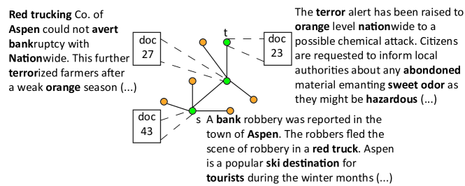
(a)

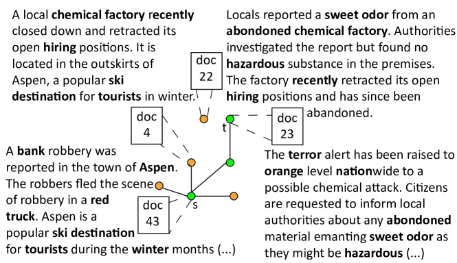
(b)

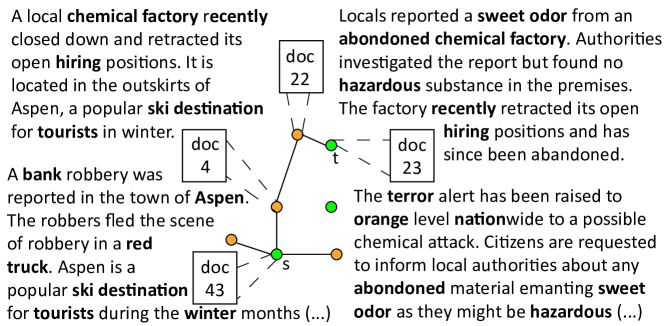
(c)

Figure 1: An illustration of the interactive storytelling algorithm.

Now consider the storytelling scenario from Fig. 1. The user desires to make a story from document $d_{43}(5\cdots 7)$ to document $d_{23}(1\cdots 3)$. $d_{43}(5\cdots 7)$ describes a bank robbery and $d_{23}(1\cdots 3)$ mentions a possible chemical attack. The constructed story is as follows: $d_{43}(5\cdots 7)\rightarrow d_{27}(1\cdots 7)\rightarrow d_{23}(1\cdots 3)$ using heuristic search (Fig. 1 (a)). The first two documents are connected using (Theme 7), involving the terms bank, red, truck, aspen. As can be seen this story is not desirable since the algorithm has conflated a bank robbery in Aspen using a red truck with the bankruptcy of the Red Trucking company (due to insufficient orange production in Aspen). Thus although the connection between two documents are established by the same set of terms, the contexts are very different.

In this case the user realizes that the story does not make very good sense, and thus uses her domain knowledge to steer the story in the right direction. She aims to incorporate a story segment $<d_{4}(5\cdots 8),d_{22}(1\cdots 8)>$ into the construction. Here, $d_{4}(5\cdots 8)$ reports the closing of a chemical factory and $d_{22}(1\cdots 8)$ mentions about a sweet odor emanating from an abandoned chemical factory (see Fig. 1 (b)). The user believes that these two documents could play an important role in the final story. Incorporating this feedback, a story from $d_{43}$ to $d_{23}$ could potentially be $d_{43}(5\cdots 7)\rightarrow d_{4}(5\cdots 8)\rightarrow d_{22}(1\cdots 8)\rightarrow d_{23}(1\cdots 3)$ (i.e., the shortest path from $d_{43}(5\cdots 7)$ to $d_{23}(1\cdots 3)$ via $d_{4}(5\cdots 8)$ and $d_{22}(1\cdots 8)$). Note that there could be other documents necessary to be included in the path that are not explicitly provided in the user’s feedback.

Incorporating this feedback, the algorithm introduced in this paper will infer new topic definitions over the dictionary of terms, and subsequently new topic distributions for each document. In this case, a new story is generated: $d_{43}(5\cdots 7)\rightarrow d_{4}(5\cdots 8)\rightarrow d_{22}(1\cdots 8)\rightarrow d_{23}(1\cdots 3)$. In this story (see Fig. 1 (c)), the first two documents are connected by the terms ski, tourist, destination, winter (Theme 5); the second and the third are linked via the terms chemical, factory, recently, hiring (Theme 8) and the last two documents are connected by nation, terror, avert, orange (Theme 1). This story thus suggests an alternative hypothesis for the user’s scenario.

Figure 2: Probability of weights of terms before (green) and after (blue) feedback. The inferred topic distributions are shifted to induce proximity between documents so that the story is consistent with user feedback.

After incorporating the user’s feedback using our proposed algorithm, we see that ski, tourist, destination, winter has some mass for document $d_{22}(1\cdots 8)$ so that it is inferred closer to document $d_{4}(5\cdots 8)$ (see Fig. 2). Similarly, the algorithm estimates positive probabilities for the terms chemical, factory, recently, hiring in document $d_{23}(1\cdots 3)$ which brings it closer to document $d_{22}(1\cdots 8)$.

3 Framework

A summary of notation as used in this paper is given in Table 1. We utilize the terms nodes and documents interchangeably in this paper. As described earlier, we impute the notion of distance between documents based on vector representations inferred from probabilistic topic models (here, LDA). Specifically, we use the topic distributions $\theta^{(d_{i}})$ and $\theta^{(d_{j})}$ for documents $d_{i}$ and $d_{j}$ (resp.) to calculate the distance or edge cost between $d_{i}$ and $d_{j}$. We posit an edge between two documents if they share any terms and the edge cost is lower than a fixed cost $\xi$. While a number of probabilistic measure of distance can be utilized, in this paper we adopt the Manhattan distance metric. The heuristic distance for a node $m$ is given by the straight line distance to the ending (target) document $t$. Since the Manhattan distance obeys the triangle inequality, it is well known that it is an admissble heuristic for A* search. As is customary, we define a node evaluation function $fScore(l)$ as the sum of $gScore(l)$ and $hScore(l)$.

Table 1: Notation overview.

Notation	Explanation
$d_{i}$	$i^{th}$ document in the copus
$T$	total number of topics
$s$	starting document
$t$	ending/goal document
$\xi$	distance threshold
$\theta^{(d_{i})}=(\theta_{1}^{(d_{i})},\cdots,\theta_{T}^{(d_{1})})$	$T$ dimensional vector of normalized topic distribution of document $d_{i}$
$e_{ij}$	edge between $d_{i}$ and $d_{j}$ if they have any term in common
$c(e_{ij})$	cost between $d_{i}$ and $d_{j}$, $c(e_{ij})=c_{ij}=\sum_{t=1}^{T}\Delta_{(ij)t}$, where $\Delta_{(ij)t}=|\theta_{t}^{d_{i}}-\theta_{t}^{d_{j}}|$
$P=<s,d_{P(1)},d_{P(2)},\cdots,d_{L-1},t>$	path $P$ from $s$ to $t$ with $L$ edges, $d_{P(i)}$ is the $i^{th}$ document after $s$
$c(P)$	$c(P)=\sum_{e_{ij}\in P}c(e_{ij})$
$P^{*}$	shortest path from $s$ to $t$
$d(i,j)$	cost of the shortest path from $i$ to $j$
$gScore(l)$	cost of the shortest path from $s$ to $l$ using $A^{*}$ search
$hScore(m)$	the heuristic distance (Manhattan distance) between the node $m$ and the goal node $t$
$\alpha_{e^{*}}$	minimum cost any $e^{*}\in E-P^{*}$ is bounded by such that $P^{*}$ is the shortest path from $s$ to $t$
$\beta_{e^{*}}$	maximum cost any $e^{*}\in P^{*}$ is bounded by such that $P^{*}$ is the shortest path from $s$ to $t$
$d^{e,k}(s,t)$	cost of the shortest path from $s$ to $t$ with $c(e)=k$
$c^{e,k}(P)$	cost of an arbitrary path $P$ with $c(e)=k$
$d(s,e,t)$	cost of the shortest path from $s$ to $t$ including an edge $e\in E$

3.1 Obtaining User Feedback

After an initial story generated by heuristic search, the user provides a sequence of documents that ought to be included in the story (i.e., between the documents $s$ and $t$). Suppose this sequence is $\mathcal{C}=<C_{1},\cdots,C_{K}>$. The order of the documents is important, since the sequence is a reflection of desired story progression. We define the path $P^{*}$ as a concatenation of the shortest path between $s$ and $C_{1}$, followed by the nodes in $\mathcal{C}$, and finally the shortest path between $C_{K}$ and $t$. This process is done in the original LDA-inferred topic space. We will now undertake a constrained $A^{*}$ search incorporating the user feedback.

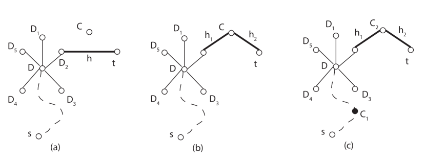
Figure 3: (a) shows the heuristic distance $h(D_{2},t)$ from original $A^{*}$ search. (b) depicts $h^{*}(D_{2},t)$ based on constrained $A^{*}$ search. (c) depicts $h^{*}(D_{2},t)$ when feedback nodes are $\mathcal{C}=<C_{1},C_{2}>$ where ancestry of $D$ is given by $\mathcal{A}(D)=C_{1}$. Dashed line shows the shortest path from $s$ to $D$.

3.2 Constrained $A^{*}$ search

Now we discuss the incorporation of the user’s feedback into the story. Consider the case where the user insists that a document $C$ (not in the initial story) should be included in the story. This case can be easily extended to a sequence of documents $\mathcal{C}=<C_{1},\cdots,C_{K}>$. Suppose the adjacent nodes of a document $d$ is denoted by $\mathcal{N}(d)$. There are five adjacent nodes to $d$ in Fig. 3. The heuristic distance between a neighbor (say, $D_{2}$) and the ending document $t$ is given by $h(D_{2},t)$ in the original $A^{*}$ search. Our redefined heuristic distance for constrained $A^{*}$ search is given by $h^{*}(D_{2},B)=h(D_{2},C)+h(C,B)$. If the feedback is a sequence of documents $\mathcal{C}=<C_{1},\cdots,C_{K}>$ then $h^{*}(D_{2},t)=h(D_{2},C_{1})+h(C_{1},C_{2})+\cdots+h(C_{K},t)$. However, while $h^{*}$ ensures that the $fScore$ of a document depends on the path via the sequence of feedback nodes $\mathcal{C}$, it must also consider the subset of $\mathcal{C}$ that already belong to the shortest path from $s$ to $D$ to estimate the heuristic distance $h^{*}(D,t)$. We define a property named Ancestry that keeps track of the subset of the feedback nodes that already exists in the shortest path from the $s$ to the said node. Ancestry $\mathcal{A}(D_{i})$ of an arbitrary neighbor of $D$ is defined as $\mathcal{A}(D_{i})=\mathcal{A}(predecessor(D))$ if $D$ is not a feedback node. If $D$ is the feedback node immediately after the subsequence $\mathcal{A}(predecessor(D))$ in $\mathcal{C}$ then $\mathcal{A}(D_{i})=\{(predecessor(D)),D\}$. The starting node $s$ has an empty ancestry. A node having longer subsequence of $\mathcal{C}$ in its ancestry compared to another is said to have a richer ancestry. A node with richer ancestry is always preferred. If ancestries are comparable, for an open node the predecessor with smaller $gScore$ is chosen while for a closed node the predecessor with smaller $fScore$ is chosen.

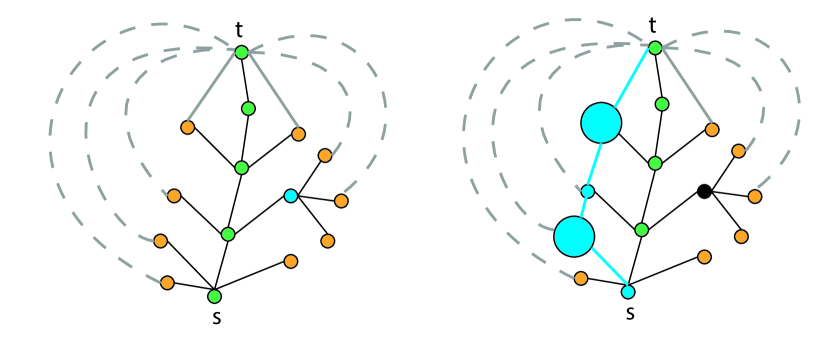
Figure 4: (left) The path with green nodes is the initial story generated by the storytelling algrithm and hence the shortest path from $s$ to $t$ before incorporating feedback. The gray paths (dashed and solid) are alternate stories abandoned by the $A^{*}$ search. (right) Story after user feedback where the user-preferred story $P^{*}$ is shown in blue. This is not the shortest path in the current topic space. The documents that the user desires to be in the story are shown in large circles. We intend to estimate the topic space where the blue path ($P^{*}$) is shorter than all the other alternate paths from $s$ to $t$.

3.3 Alternate/Candidate Stories

The nodes explored by $A^{*}$ search in the initial topic space (the set of open and closed nodes) induce an acyclic graph $G(V,E)$. The orange nodes in Fig. 4 are open nodes in such a graph. Denote the set of open nodes by $\mathcal{O}$. Any path from $s$ to $t$ via $o\in\mathcal{O}$ is a candidate story generated by $A^{*}$ search. Let us denote the path via $o$ by $P^{(o)}$.

Now assume $\mathcal{O}$ has $O$ open nodes. To enforce the user feedback that $P^{*}$ be the shortest path over all paths from $s$ to $t$ we define the following system of inequalities:

$$c(P^{*}) \leq c(P^{(o_{1})})$$

$$\vdots$$

$$c(P^{*}) \leq c(P^{(o_{O})})$$ (1)

If we break each inequality in terms of topics then we obtain:

$$\sum_{t=1}^{T}(\Delta_{t}^{*}-\Delta^{(o_{1})}) \leq 0$$

$$\vdots$$

$$\sum_{t=1}^{T}(\Delta_{t}^{*}-\Delta^{(o_{O})}) \leq 0$$ (2)

In addition to this set of inequalities, we also add another set of inequalities imposing that the cost of an edge in the new topic space, $c(e)$ is at least as much as the cost of the edge in the initial topic space $c_{0}(e)$.

$$c(e)\geq c_{0}(e),e\in E$$ (3)

This constraint is imposed so that the proximity of the document does not change drastically, as otherwise this might disorient users.

3.4 Deriving Systems of Inequalities

$A^{*}$ is a heuristic algorithm to find the shortest path between two nodes. Given the shortest path, finding the edge costs or upper and lower limits thereof is thus as inverse shortest path problem. Our goal is to find a normalized topic distribution $\theta^{(d_{i})}$ so that $P^{*}$ is actually the shortest path in the new topic space.

In our approach, we obtain the inequalities in Eqn 2 by using the following observation: if the cost of an edge $e^{*}\in P^{*}$ crosses the upper threshold $\beta_{e}^{*}$ or an edge $e\not\in P^{*}$ falls below the lower threshold $\alpha_{e}$, all the other edge cost being fixed $P^{*}$ is no longer the shortest path from $s$ to $t$. Therefore the condition for $P^{*}$ being the shortest path is

$$c(e^{*})\leq\beta_{e}^{*},\forall e^{*}\in P^{*}$$

$$c(e)\geq\alpha_{e},\forall e\in E-P^{*}$$ (4)

Upper and lower shortest path tolerances are presented in [25] as:

$$\beta_{e^{*}} =d^{e^{*},\infty}(s,t)-c(P^{*})+c(e^{*})$$

$$\alpha_{e} =c(P^{*})-d^{e,0}(s,t)$$ (5)

Therefore the inequities for the edges becomes:

$$c(P^{*}) \leq d^{e^{*},\infty}(s,t),\forall e^{*}\in P^{*}$$ (6)

$$c(e) \geq c(P^{*})-d^{e,0}(s,t),\forall e\in E-P^{*}$$ (7)

Note that for the first equation in Eqn. 3.4, $\beta_{e^{*}}$ is the difference of two path costs: the cost of the shortest path from $s$ to $t$ that avoid $e^{*}$ (imposing an infinite cost for $e^{*}$) $d^{e^{*},\infty}(s,t)$ and the minimum cost of $P^{*}$ with $e^{*}$ in the path (imposing a zero cost for $e^{*}$), so that $c(P^{*})-c(e^{*})=c^{e^{*},0}(P^{*})$. Notice also that if $e=(l,m)$, then $d^{e,o}(s,t)=\min(c(P^{*}),d(s,l)+d(m,t))$. For the second equation if the shortest path from $s$ to $t$ does not change even with $c(e)=0$, i.e. $d^{e,0}(s,t)=c(P^{*})$, then the lower tolerance for $c(e)$ is zero. However, if the constraint $c(e)=0$ favors a different path through $e$ (meaning not $P^{*}$) the lower tolerance for $e$ is given by the drop in the path cost which this alternate path allows over $P^{*}$.

We use the fact that our choice of $hScore$ is an admissible heuristic in $A^{*}$ search to simplify our formulation of inequalities. Due to admissibility, $hScore(m)\leq d(m,t)$, and consequently $gScore(l)+hScore(m)\leq d(s,l)+d(m,l)$. Replacing $d^{e,0}(s,t)$ with lower heuristic estimate of $gScore(l)+hScore(m)$ in Eqn. 7 we achieve a stricter inequality:

$$\left.\begin{matrix}c(e)\geq c(P^{*})-gScore(l)-hScore(m)\\ c(e)\geq 0\end{matrix}\right\}\forall e\in E-P^{*}$$ (8)

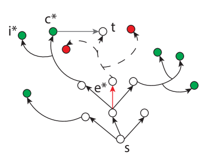
Figure 5: Dashed line shows the subtree $\tau(e^{*})$ and the solid line shows the subtree $\tau^{C}(e^{*})$. The candidate open nodes in $\tau^{C}(e^{*})$ for Eqn. 6 are shown in green. Red nodes are open nodes in $\tau(e^{*})$ and do not contribute in Eqn. 6. The shortest path from $s$ to $t$ avoiding $e^{*}$ is the shortest path from $s$ to $t$ via any of the green nodes.

The cost of shortest path avoiding $e^{*}\in P^{*}$ is given by $d^{e^{*},\infty}(s,t)=\min_{e\in E-P^{*}}(d(s,e,t)|e^{*}\not\in d(s,e,t))$. In Fig. 5 suppose the red edge is one such $e^{*}\in P^{*}$. Let the subtree induced by $A^{*}$ search following $e^{*}$ is $\tau(e^{*})$ (shown in dashed line) and the remainder of the tree is $\tau^{C}(e^{*})$ (shown in solid line). Based on the search process, we would expect the shortest path from $s$ to $t$ via any edge in $\tau(e^{*})$ to have $e^{*}$ in it. Therefore $d^{e^{*},\infty}(s,t)$ should be based on paths via edges in $\tau^{C}(e^{*})$. Since we have path costs that are estimated by the heuristically $A^{*}$ search ($fScores$) we can use these for the open nodes in $\tau^{C}(e^{*})$. These open nodes are shown in green in Fig. 5. Hence in this setting, the inequality $c(P^{*})\leq\min_{e\in E-P^{*}}(d(s,e,t)|e^{*}\not\in d(s,e,t))$ is replaced by the following set of inequalities:

$$c(P^{*})\leq fScore(o),\forall o\text{ in the set of open nodes in }\tau^{C}(e^{*})$$ (9)

Due to the admissibility of $hScore$, $fScore$ also underestimates the true distance, so we are using a stricter inequality in Eqn. 9. If this process is repeated for all $e^{*}\in P^{*}$ our set of inequalities consist of the user defined path $P^{*}$ being compared against all the set of paths defined by the open nodes in the original $A^{*}$ search given in Eqn 2.

3.5 Modeling Relationships by Auxiliary Variables

In the previous section we formulated the user feedback as a set of relationships, where each relationship is an inequality in terms of path lengths. Since the distance metric is based on normalized topic distribution we explicitly show the dependence of an individual relationship on $\boldsymbol{\theta}$. For an inequality $r_{o}\equiv c(P^{*})\leq c(P^{(o)})$ in Eqn. 2, we introduce a slack random variable $\lambda_{o}$ (i.e. $\lambda_{o}\leq\epsilon$ for some $\epsilon\leq 0$) as an auxiliary variable with expectation $\boldsymbol{E}(\lambda_{o})=\mu_{o}(\boldsymbol{\theta})=c(P^{*})-c(P^{(o)})$. Similarly for a relationship $r_{e}\equiv c(e)\geq c_{0}(e)$ in Eqn 3 we define a surplus random variable $\lambda_{e}$ where $\lambda_{e}$ is positive with expectation given by $\boldsymbol{E}(\lambda_{e})=\mu_{o}(\boldsymbol{\theta})=c(e)-c_{0}(e)$. Therefore $\mu_{o}(\boldsymbol{\theta})=\sum_{t=1}^{T}(\Delta_{t}^{*}(\boldsymbol{\theta})-\Delta_{t}^{(o)}(\boldsymbol{\theta}))$. Suppose the distribution of the auxiliary variable is given by $\lambda_{o}\sim f(\cdot|\boldsymbol{\theta})$. The random variable $\lambda_{o}$ measures the difference in path lengths between the user defined path $P^{*}$ and an alternate $P^{(o)}$. If $\mu_{o}(\boldsymbol{\theta})$ is zero, it means enforcing the relationship that $P^{*}$ is as costly as the alternate path $P^{(o)}$. The more negative the value of its mean $\mu_{o}(\boldsymbol{\theta})$, the larger we expect $P^{(o)}$ to be compared to $P^{*}$. This ensures that the topic space $\boldsymbol{\theta}$ satisfies the relationship $c(P^{*})\leq c(P^{(o)})$. Now conditional on a known $\boldsymbol{\theta}$, the joint distribution of the auxiliary variables (both slack and surplus) and the observed feedback $\Re$ is given below:

$$\begin{split}f(\Re,\boldsymbol{\lambda}|\boldsymbol{\theta})&\propto\prod_{o\in\mathcal{O}}\{\mathbbm{1}_{c(P^{*})\leq c(P^{(o)}}\mathbbm{1}_{\lambda_{o}\leq\epsilon}+\mathbbm{1}_{c(e)\geq c_{o}(e)}\mathbbm{1}_{\lambda_{0}\geq 0}\}f(\lambda_{o}|\boldsymbol{\theta})\end{split}$$ (10)

Here, $\mathbbm{1}_{x}$ is an indicator variable which is one if condition $x$ holds and zero otherwise. Our goal is to find a set of surplus and slack variables $\boldsymbol{\lambda}$ that maximizes the probability in Eqn 10. Now let $f(\lambda_{o}|\boldsymbol{\theta})$ be normally distributed with mean $\mu_{0}(\boldsymbol{\theta})$ and variance 1. By marginalizing over the auxiliary variables $\lambda_{o}$, our formulation is same as the modeling the probability of satisfying a relationship using the cumulative normal distribution.

$$P(c(P^{*})\leq c(P^{(o)})|\boldsymbol{\theta}) =1-\Phi(\mu_{o}(\boldsymbol{\theta})-\epsilon),\text{for Eqn \ref{eqn:inqT}}$$

$$P(c(e)\geq c_{0}(e)|\boldsymbol{\theta}) =\Phi(\mu_{o}(\boldsymbol{\theta})),\text{for Eqn \ref{eqn:e}}$$ (11)

Here for a standard normal variable $Z$, $\Phi(z)=P(Z\leq z)$. This approach is very similar to the usage of auxiliary variables in probit regression [1]. In probit regression the mean of the auxiliary variable is modeled by a linear predictor to maximize the discrimination between the successes and failures in the data. In our case satisfiability of a user defined relationship is a success and the probability of satisfying the relationship is modeled by the mean of auxiliary variable. The mean of the auxiliary variable is a function of the topic space $\boldsymbol{\theta}$ on which the distances are defined. Our goal is to search for a topic space $\boldsymbol{\theta}$ which explains the term distribution of the documents and satisfies as many of the relationships in $\Re$ as possible. Truncating a slack variable $\lambda_{o}$ to a negative region specified by $\epsilon$ allows to search for $\boldsymbol{\theta}$ that shrinks the mean $\mu_{o}(\boldsymbol{\theta})$ to a negative value. The complete hierarchical model using the term document data $\boldsymbol{\eta}$ and the relationship data $\Re$ is presented below:

$$\begin{split}f(\Re,\boldsymbol{\lambda}|\boldsymbol{\theta})&\propto\prod_{o\in\mathcal{O}}\{\mathbbm{1}_{c(P^{*})\leq c(P^{(o)}}\mathbbm{1}_{\lambda_{o}\leq\epsilon}+\mathbbm{1}_{c(e)\geq c_{o}(e)}\mathbbm{1}_{\lambda_{o}\geq 0}\}N(\lambda_{o}|\mu_{o}(\boldsymbol{\theta}),1)\end{split}$$

$$\eta_{i}|z_{i},\phi^{(z_{i})} \sim Discrete(\phi^{(z_{i})})$$

$$\phi \sim Dirichlet(\beta)$$

$$z_{i}|\theta^{(d_{i})} \sim Discrete(\theta^{(d_{i})})$$

$$\theta \sim Dirichlet(\alpha)$$ (12)

3.6 Inference

We use Gibbs sampling to compute the posterior distributions for $\mathbf{z},\boldsymbol{\lambda}$ and $\boldsymbol{\theta}$. The conditional posterior distributions for $z_{i}$ is given below:

$$p(z_{i}=j|\mathbf{z}_{(-i)},\boldsymbol{\eta})\propto p(\eta_{i}|z_{i}=j,\mathbf{z}_{(-i)},\boldsymbol{\eta}_{(-i)})p(z_{i}=j|\mathbf{z}_{(-i)},\boldsymbol{\eta}_{(-i)})$$ (13)

The sampling of topic for terms $\boldsymbol{\eta}$ is same as used in vanilla LDA [11].

$$p(z_{i}=j|\mathbf{z}_{(-i)},\boldsymbol{\eta})\propto\dfrac{\beta+n^{(\eta_{i})}_{(-i,j)}}{M\beta+n^{(\cdot)}_{(-i,j)}}\times\dfrac{\alpha+n_{(-i,j)}^{(d_{i})}}{T\alpha+n_{(-i,\cdot)}^{(d_{i})}}$$ (14)

The full conditional distribution for $\lambda_{o}$ is given below:

$$p(\lambda_{o}|\boldsymbol{\theta},\Re)=\begin{cases}N(\cdot|\mu_{o}(\boldsymbol{\theta}),1),\lambda_{o}\leq\epsilon,\text{if }r_{o}\text{ is }\leq\text{ type}\\ N(\cdot|\mu_{o}(\boldsymbol{\theta}),1),\lambda_{o}>0,\text{if }r_{o}\text{ is }>\text{ type}\end{cases}$$ (15)

The full conditional distribution for the topic distribution of document $d_{j}$ is given below:

$$\begin{split}p(\theta^{(d_{j})}|\boldsymbol{\theta}^{(-d_{j})},\boldsymbol{\lambda},\boldsymbol{z})&\propto\prod_{z_{i}\in d_{j}}p(z_{i}|\theta^{(d_{j})})p(\theta^{(d_{j})}|\alpha)\times\prod_{o\in\mathcal{O}}N(\lambda_{o}|\mu_{o}(\boldsymbol{\theta}),1)\end{split}$$

$$\propto p(\theta^{(d_{j})}|\boldsymbol{z},\alpha)\prod_{o\in\mathcal{O}}N(\lambda_{o}|\mu_{o}(\boldsymbol{\theta}),1)$$

$$\propto\prod_{t=1}^{T}\left(\theta_{t}^{(d_{j})}\right)^{(n_{t}^{(d_{j})}+\alpha)-1}\prod_{o\in\mathcal{O}}N(\lambda_{o}|\mu_{o}(\boldsymbol{\theta}),1)$$ (16)

since $p(\theta^{(d_{j})}=Dirichlet(n_{t}^{(d_{j})}+\alpha)$. $n_{t}^{(d_{j})}$ denotes the number of terms in document $d_{j}$ assigned to topic $t$ based on $\boldsymbol{z}$. If $d_{j}$ does not belong to $\Re$, then $\theta^{(d_{j})}$ is sampled from $Dirichlet(n_{t}^{(d_{j})}+\alpha)$. We sample from $p(\theta^{(d_{j})}|\boldsymbol{\theta}^{(-d_{j})},\boldsymbol{\lambda},\boldsymbol{z})$ by a Metropolis-Hastings step otherwise. We use a proposal strategy based on stick-breaking process to allow better mixing. The stick-breaking process bounds the topic distribution of a document $d_{j}$ between zero and one and their sum to one. We first sample random variables $u_{1},\cdots,u_{T-1}$ truncated between zeros and one and centered by $\boldsymbol{\theta}^{(d_{j})}$ using a proposal distribution $q(\cdot)$:

$$u_{1} \sim q\left(\cdot|\theta_{1}^{(d_{j})}\right),0<u_{1}<1$$

$$u_{2} \sim q\left(\cdot|\dfrac{\theta_{2}^{(d_{j})}}{1-u_{1}}\right),0<u_{2}<1$$

$$u_{3} \sim q\left(\cdot|\dfrac{\theta_{3}^{(d_{j})}}{(1-u_{1})(1-u_{2})}\right),0<u_{3}<1$$

$$\vdots$$

$$u_{T-1} \sim q\left(\cdot|\dfrac{\theta_{T-1}^{(d_{j})}}{(1-u_{1})(1-u_{2})\cdots(1-u_{T-2})}\right),0<u_{T-1}<1$$ (17)

This is followed by the mappings, $S:\mathbf{u}\rightarrow\boldsymbol{\theta}_{1:T-1}^{*(d_{j})}$,

$$\theta_{1}^{*(d_{j})} =u_{1}$$

$$\theta_{2}^{*(d_{j})} =u_{2}(1-u_{1})$$

$$\theta_{3}^{*(d_{j})} =u_{3}(1-u_{2})(1-u_{1})$$

$$\vdots$$

$$\theta_{T-1}^{*(d_{j})} =(1-u_{T-1})(1-u_{T-2})\cdots(1-u_{2})(1-u_{1})$$ (18)

The inverse mappings $S^{-1}:\boldsymbol{\theta}_{1:T-1}^{*(d_{j})}\rightarrow\mathbf{u}$ are given by:

$$u_{1} =\theta_{1}^{*(d_{j})}$$

$$u_{t} =\dfrac{\theta_{1}^{*(d_{j})}}{1-\sum_{i<t}\theta_{i}^{*(d_{j})}},t=2,\cdots T-1$$ (19)

The Metropolis-Hastings acceptance probability for such a proposed move is given by

$$\begin{split}p_{MH}&=\min\left(1,\dfrac{(p(\theta^{*(d_{j})})|\mathbf{z})\prod_{o\in\mathcal{O}}N(\lambda_{o}|\mu_{o}(\boldsymbol{\theta}^{*}),1))}{(p(\theta^{(d_{j})})|\mathbf{z})\prod_{o\in\mathcal{O}}N(\lambda_{o}|\mu_{o}(\boldsymbol{\theta}),1))}\times\right.\left.\dfrac{q(\boldsymbol{\theta}^{*(d_{j})}_{1:T-1})}{q(\mathbf{u})}\left|\dfrac{\delta(\boldsymbol{\theta}^{*(d_{j})}_{1:T-1})}{\delta(\mathbf{u})}\right|\right)\end{split}$$ (20)

where $\left|\dfrac{\delta(\boldsymbol{\theta}^{*(d_{j})}_{1:T-1})}{\delta(\mathbf{u})}\right|=\left|\dfrac{\delta(\mathbf{u})}{\delta(\boldsymbol{\theta}^{*(d_{j})}_{1:T-1})}\right|^{-1}$=$\left(\dfrac{1}{\prod_{t=2}^{T-1}\left(1-\sum_{i<t}\theta_{i}^{*(d_{j})}\right)}\right)$ The samples from $\mathbf{z},\boldsymbol{\lambda}$ and $\boldsymbol{\theta}$ are iteratively sampled to generate the joint posterior distribution of all the unknown parameters using Gibbs Sampling.

This procedure completes the interactivity loop in the storytelling algorithm. The newly inferred topic distributions will induce a new similarity network over which we can again conduct a search, followed by (potentially) additional user feedback.

4 Experimental Results

We evaluate our interactive storytelling approach over a range of text datasets from intelligence analysis, such as Atlantic Storm, Crescent, Manpad, and the VAST11 dataset from the IEEE Visual Analytics Science & Technology Conference. Pl see [35] for details of these datasets. The questions we seek to answer are:

1. Can we effectively visualize the operations of the interactive storytelling as user feedback is incorporated? (Section 4.1)

2. Does the interactive storytelling framework provide better alternatives for stories than a vanilla topic model? (Section 4.2)

3. Are topic reoorganizations obtained from interactive storytelling significantly different from a vanilla topic model? (Section 4.3)

4. Does our method scale to large datasets? (Section 4.4)

5. How effectively does the interactive storytelling approach improve over uninformed search (e.g., uniform cost search or breadth-first search)? (Section 4.5)

In the below, unless otherwise stated, we fix the number of topics to be $T=20$ and set $\alpha=0.05/T$ and $\beta=0.01$. We also use the Gini index to remove top 10% of of the terms as a pre-processing step for our text collections.

4.1 Visualizing interactive storytelling

We apply multidimensional scaling (MDS) over the normalized topic space as an aid to visualize the operations of the storytelling algorithm. For instance, the Manpad dataset is visualized as shown in Fig. 6. Consider a story from document $Doc$-$29$ to document $Doc$-$26$. Here $Doc$-$29$ reports that a member of an infamous terrorist organization has a meeting with a notorious arms dealer. $Doc$-$26$ reports that a team of suicide bombers plans to set off bombs in trains carrying tens of thousands of commuters under the Hudson River. The storytelling algorithms generates a story as: $Doc$-$29\rightarrow Doc$-$32\rightarrow Doc$-$26$. Here, $Doc$-$32$ identifies a person belong to a terrorist organization. The user is not satisfied with this story and provides a constraint that the story should involve documents $Doc$-$44$ and $Doc$-$49$. Here, $Doc$-$44$ describes that libraries in Georgia and Colorado have some connections to a web site. $Doc$-$49$ reports that a code number is found in the website linked to a charitable organization. Using this feedback a new story is generated: $Doc$-$29\rightarrow Doc$-$44\rightarrow Doc$-$49\rightarrow Doc$-$16\rightarrow Doc$-$26$. In addition to being consistent with the user’s feedback, note that the algorithm has introduced a new document ($Doc$-$16$) which contains a report of police seizing documents involving specific names and dates.

4.2 Evaluating story options

In this experiment, we seek to generate multiple stories using our interactive storytelling approach as well as a vanilla topic modeling, with a view to comparative evaluation. In this experiment, run over the Atlantic Storm dataset, the user specifies $CIA06$ as the starting document and $NSA16$ as the ending document. The default story is: $CIA06\rightarrow CIA37\rightarrow NSA19\rightarrow NSA16$. The user’s feedback specifies $CIA08$ and $NSA09$ to be included in the final story. The results of incorporating this feedback yields: $CIA06\rightarrow CIA08\rightarrow DIA01\rightarrow NSA09\rightarrow NSA16$. We next use Yen’s $k$-shortest path algorithm [20] to generate a set of top $10$ (alternative) stories. As shown in Table 2, the top-ranked path in the interactive setting is indeed the shortest path in the new topic space that satisfies the given constraints.

Table 2: Top $10$ stories (shortest paths) generated from $CIA06$ to $NSA16$ using both a vanilla topic model and the interactive storytelling algorithm (using the Atlantic Storm dataset). The user’s feedback requires that both $CIA08$ and $NSA09$ be included in the story. The interactive storytelling algorithm updates the topic model wherein the shortest path indeed contains these documents.

Top $10$ stories generated using vanilla topic model	Path Length	Top $10$ stories generated using interactive storytelling	Path Length
CIA06, CIA37, NSA19, NSA16	2.84	CIA06, CIA08, DIA01, NSA09, NSA16	1.39
CIA06, CIA20, CIA21, NSA16	3.16	CIA06, CIA12, NSA09, NSA16	1.93
CIA06, CIA22, CIA21, NSA16	3.16	CIA06, CIA33, DIA01, NSA09, NSA16	2.13
CIA06, CIA20, CIA22, CIA21, NSA16	3.16	CIA06, CIA22, NSA09, NSA16	2.13
CIA06, CIA22, CIA20, CIA21, NSA16	3.16	CIA06, CIA08, DIA01, FBI07, NSA16	2.20
CIA06, CIA08, NSA21, NSA16	3.23	CIA06, CIA33, FBI07, NSA16	2.22
CIA06, CIA08, NSA21, NSA12, NSA16	3.23	CIA06, CIA33, CIA08, DIA01, NSA09, NSA16	2.31
CIA06, CIA08, NSA21, NSA13, NSA16	3.23	CIA06, CIA11, FBI13, DIA01, NSA09, NSA16	2.33
CIA06, CIA08, NSA21, NSA12, NSA13, NSA16	3.23	CIA06, DIA02, DIA01, NSA09, NSA16	2.33
CIA06, CIA08, NSA21, NSA18, NSA16	3.23	CIA06, CIA08, CIA23, NSA16	2.34

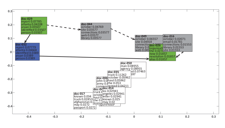
Figure 6: Visualizing documents using multidimensional scaling (Manpad dataset) before and after user feedback. Many documents are omitted for better visualization. The starting and the ending documents are shown in green. The documents in the initial story are shown in blue (and the story by solid lines). The story generated by the interactive storytelling algorithm is shown in the dotted line through the grey documents. Each document is represented by its top five terms having the highest posterior probability.

4.3 Proximity between topics

We investigate topic proximity in terms of Manhattan distance in Fig  7. Here, rows denote topics from a vanilla topic model, and the columns correspond to topics inferred by the interactive storytelling algorithm. As shown in Fig. 7 the diagonally dominant nature of the matrix is destroyed due to the introduction of user feedback, illustrating that the distributions of words underyling the topics are quite dissimilar.

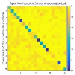
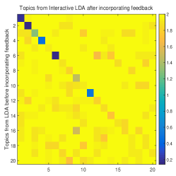
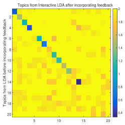
Atlantic Storm	Crescent	Manpad

Figure 7: Manhattan distance between topic distributions before and after user feedback. Blue color denotes topics closest to each other. As can be seen, the incorporation of feedback destroys the diagonal dominance of the matrix.

4.4 Scalability to large corpora

With large datasets, such as the VAST11 dataset, we can fruitfully combine clustering with our framework to navigate the document collection (see Fig. 8). Given a document collection, an initial clustering (e.g., k-means) can be utilized to identify broad groups of documents that can be discarded during the initial story construction. Here, assume that the user specifies $00795.txt$ and $00004.txt$ as the starting and ending document, respectively. The storytelling algorithm generates $00795.txt\rightarrow 014171.txt\rightarrow 00004.txt$ as the initial story (solid line). Note that this story ignores documents from the cluster displayed in red. Assume that the user now requires that documents from the red cluster also participate in the story. Based on an initial exploratory analysis, the user specifies that documents $02247.txt$ and $00082.txt$ should participate in the story. Based on this feedback the interactive storytelling algorithm generates: $00795.txt\rightarrow 01486.txt\rightarrow 02247.txt\rightarrow 00082.txt\rightarrow 04134.txt\rightarrow 00004.txt$ (note the introduction of $04134.txt$ into the story).

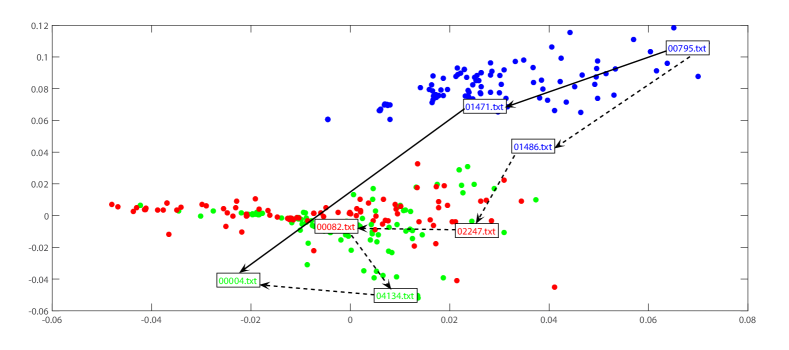
Figure 8: Scaling the storytelling methodology by integrating clustering. The initial story (solid line) from $00795.txt$ to $00004.txt$ avoided documents in the red cluster. After incorporating user feedback, the new story (dotted line) navigates through the red cluster.

4.5 Comparing interactive storytelling vs uniform cost search

We now assess the performance of the constrained search process underlying interactive storytelling versus that of an uninformed search (e.g., uniform cost search). The comparison is shown in Fig. 9. We use different distance threshold $\xi$ to compute effective branching factor, path length and execution time.

We show in Fig. 9(a, b, c) that average effective branching factor increases with $\xi$. Since higher $\xi$ means a node will have more neighbors, the branching factor will increase in this case. However in case of Interactive Storytelling path finding is more guided so the average effective branching factor does not vary much. We can see that using a heuristics decreases the average effective branching factor. The average path length however decreases with increasing $\xi$ (Fig. 9(d, e, f)). Increasing $\xi$ results in having larger neighborhood for each node, therefore the chance of reaching the goal becomes higher resulting in shorter average path length. For Interactive Storytelling the average path length is higher because it has to visit the nodes specified by the user while searching for the shortest path. The execution time for both heuristic search and the uninformed search are almost same (Fig. 9(g, h, i)), however for Interactive Storytelling it is much longer. Since it has to visit the nodes provided by the user, it travels the search space in more depth so it takes more time on average to finish the search.

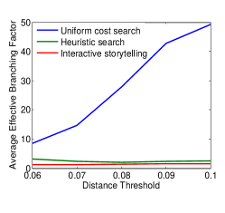
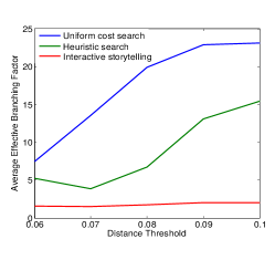
(a)	(b)	(c)
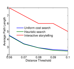
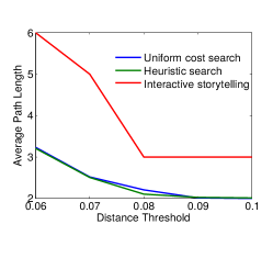
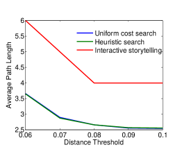
(d)	(e)	(f)
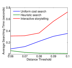
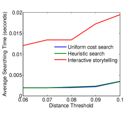
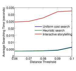
(g)	(h)	(i)

Figure 9: Comparison of interactive storytelling, heuristic search and uniform cost search in terms of average effective branching factor (top), average path length (middle) and execution time (bottom). (Left) Atlantic Storm. (middle) Crescent. (right) Manpad.

5 Related Work

Related work pertaining to storytelling has been covered in the introduction. We survey topic modeling related work here. To the best of our knowledge, no existing work supports the incorporation of path-based constraints to refine topic models, as done here.

Expressive topic models

The author-topic model [26] is one of the popular extensions of topic models that aims to model how multiple authors contributed to a document collection. Works such as [7, 6] extend basic topic modeling to include specific words or semantic concepts by incorporating notions of proximity between documents. In [32], the authors move beyond bag-of-words assumptions and accommodate the ordering of words in topic modeling. Domain knowledge is incorporated in [2] in the form of Dirichlet forest priors. Finally, in [3], correlated topic models are introduced to model correlations between topics.

Incorporating external information

Supervised topic models are introduced in [21]. Lu and Zhai [19] propose a semi-supervised topic model to incorporate expert opinions into modeling. In [24], authors incorporate user tags accorded to documents to place constraints on topic inference. The timestamps of documents is used in [4, 33] to model the evolution of topics in large corpus.

Visualizing topics

Wei et al. [34] propose TIARA, a visual exploratory text analytics system to observe the evolution of topics over time in a corpus. Crossno et al. [8] develop a framework to visually compare document contents based on different topic modeling approaches. In [22], the authors present documents in topic space and depict inter-document connectivity as a network in a visual interface, simultaneously displaying community clustering.

Interactive topic modeling

User feedback is incorporated in [16] wherein users can provide constraints about specific words that must appear in topics. An active learning framework to incorporate user feedback and improve topic quality is introduced in [36].

6 Discussion

We have demonstrated interactive storytelling, a combination of interactive topic modeling and constrained search wherein documents are connected obeying user constraints on paths. User feedback is pushed deep into the computational pipeline and used to refine the topic model. Through experiments we have demonstrated the ability of our approach to provide meaningful alternative stories while satisfying user constraints. In future work, we aim to generalize our framework to a multimodal network representation where entities of various kinds are linked through a document corpus, so that constraints can be more expressively communicated.

References

- [1] J. Albert and S. Chib. Bayesian analysis of binary and polychotomous response data. J. Amer. Statist. Assoc, 88(422):669–679, 1993.
- [2] D. Andrzejewski, X. Zhu, and M. Craven. Incorporating domain knowledge into topic modeling via dirichlet forest priors. In ICML, pages 25–32, 2009.
- [3] D. Blei and J. Lafferty. Correlated topic models. In ICML, pages 113–120, 2006.
- [4] D. Blei and J. Lafferty. Dynamic topic models. In ICML, pages 113–120, 2006.
- [5] D. Blei, A. Ng, and M. Jordan. Latent Dirichlet Allocation. JMLR, 3:993–1022, 2003.
- [6] C. Chemudugunta, A. Holloway, P. Smyth, and M. Steyvers. Modeling documents by combining semantic concepts with unsupervised statistical learning. In ISWC, pages 229–244, 2008.
- [7] C. Chemudugunta, P. Smyth, and M. Steyvers. Modeling general and specific aspects of documents with a probabilistic topic model. In NIPS, pages 241–248, 2006.
- [8] P. Crossno, A. Wilson, T. Shead, and D. Dunlavy. Topicview: Visually comparing topic models of text collections. In International Conference on Tools with Artificial Intelligence, pages 936–943, 2011.
- [9] A. Feng and J. Allan. Incident threading for news passages. In CIKM, pages 1307–1316, 2009.
- [10] S. Gad, W. Javed, S. Ghani, N. Elmqvist, E. Ewing, K. Hampton, and N. Ramakrishnan. Themedelta: Dynamic segmentations over temporal topic models. IEEE Trans. Vis. Comput. Graph., 21(5):672–685, 2015.
- [11] T. Griffiths and M. Steyvers. Finding scientific topics. PNAS, 101(suppl 1):5228–5235, 2004.
- [12] M. Hossain, C. Andrews, N. Ramakrishnan, and C. North. Helping intelligence analysts make connections. In Scalable Integration of Analytics and Visualization, volume WS-11-17, 2011.
- [13] M. Hossain, P. Butler, A. Boedihardjo, and N. Ramakrishnan. Storytelling in entity networks to support intelligence analysts. In KDD, pages 1375–1383, 2012.
- [14] M. Hossain, J. Gresock, Y. Edmonds, R. Helm, M. Potts, and N. Ramakrishnan. Connecting the dots between PubMed abstracts. PLoS ONE, 7:e29509, 01 2012.
- [15] M. Hossain, M. Narayan, and N. Ramakrishnan. Efficiently discovering hammock paths from induced similarity networks. CoRR, abs/1002.3195, 2010.
- [16] Y. Hu, J. Boyd-Graber, and B. Satinoff. Interactive topic modeling. In ACL, pages 248–257, 2011.
- [17] D. Kumar, N. Ramakrishnan, R. Helm, , and M. Potts. Algorithms for storytelling. In KDD, pages 604–610, 2006.
- [18] S. Leman, L. House, D. Maiti, A. Endert, and C. North. Visual to parametric interaction (v2pi). PLoS ONE, 8(3), 2013.
- [19] Y. Lu and C. Zhai. Opinion integration through semi-supervised topic modeling. In WWW, pages 121–130, 2008.
- [20] E. Martins and M. Pascoal. A new implementation of yen’s ranking loopless paths algorithm. 4OR, 1:121–133, 2003.
- [21] J. Mcauliffe and D. Blei. Supervised topic models. In NIPS, pages 121–128, 2008.
- [22] Q. Mei, D. Cai, D. Zhang, and C. Zhai. Topic modeling with network regularization. In WWW, pages 101–110, 2008.
- [23] R. Nallapati, A. Feng, F. Peng, and J. Allan. Event threading within news topics. In CIKM, pages 446–453, 2004.
- [24] D. Ramage, D. Hall, R. Nallapati, , and C. Manning. Labeled lda: A supervised topic model for credit attribution in multi-labeled corpora. In EMNLP, pages 248–256, 2009.
- [25] R. Ramaswamy, J. B. Orlin, and N. Chakravarti. Sensitivity analysis for shortest path problems and maximum capacity path problems in undirected graphs. Math. Program, 102(2):355–369, 2005.
- [26] M. Rosen-Zvi, T. Griffiths, M. Steyvers, and P. Smyth. The Author-Topic model for authors and documents. In UAI, pages 487–494, 2004.
- [27] D. Shahaf and C. Guestrin. Connecting the dots between news articles. In KDD, pages 623–632, 2010.
- [28] D. Shahaf and C. Guestrin. Connecting two (or less) dots: Discovering structure in news articles. ACM Trans. Knowl. Discov. Data, 5(4):24:1–24:31, 2012.
- [29] D. Shahaf, C. Guestrin, and E. Horvitz. Metro maps of science. In KDD, pages 1122–1130, 2012.
- [30] D. Shahaf, C. Guestrin, and E. Horvitz. Metro maps of information. SIGWEB Newsletter, 2013.
- [31] D. Shahaf, J. Yang, C. Suen, J. Jacobs, H. Wang, and J. Leskovec. Information cartography: Creating zoomable, large-scale maps of information. In KDD, pages 1097–1105, 2013.
- [32] H. Wallach. Topic modeling: Beyond bag-of-words. In ICML, pages 977–984, 2006.
- [33] X. Wang and A. McCallum. Topics over time: A non-markov continuous-time model of topical trends. In KDD, pages 424–433, 2006.
- [34] F. Wei, S. Liu, Y. Song, S. Pan, M. Zhou, W. Qian, L. Shi, L. Tan, and Q. Zhang. Tiara: A visual exploratory text analytic system. In KDD, pages 153–162, 2010.
- [35] H. Wu, M. Mampaey, N. Tatti, J. Vreeken, M. Hossain, and N. Ramakrishnan. Where do I start?: Algorithmic strategies to guide intelligence analysts. In KDD Workshop on Intelligence and Security Informatics, pages 3:1–3:8, 2012.
- [36] Y. Yang, S. Pan, D. Downey, and K. Zhang. Active learning with constrained topic model. Sponsor: Idibon, 2014.