Scrambling without chaos in RCFT

Abstract

In this paper we investigate measures of chaos and entanglement in rational conformal field theories in 1 + 1 dimensions. First, we derive a formula for the late time value of the out-of-time-ordered correlators for this class of theories. Our universal result can be expressed as a particular combination of the modular S-matrix elements known as anyon monodromy scalar. Next, in the explicit setup of an $SU(N)_{k}$ Wess–Zumino–Witten model, we compare the late time behavior of the out-of-time-ordered correlators and the purity. Interestingly, in the large-$c$ limit, the purity grows logarithmically as in holographic theories; in contrast, the out-of-time-ordered correlators remain, in general, nonvanishing.

I Introduction

Two-dimensional conformal field theories (2d CFTs) have played an important role in understanding a number of interesting questions in theoretical physics. In this vein they’ve become central tools in the study of entanglement Calabrese:2004eu and more recently quantum chaos. Based on earlier work on superconductors by Larkin and Ovchinnikov LO , Kitaev has proposed that chaotic behavior in quantum systems can be diagnosed by computing the expectation value of the square of commutators of local operators Kitaev . This essentially amounts to calculating the out-of-time order thermal correlator (OTOC)

$$C_{ij}^{\beta}(t)\equiv{\left<\mathcal{O}_{i}^{\dagger}(t)\mathcal{O}^{\dagger}_{j}\mathcal{O}_{i}(t)\mathcal{O}_{j}\right>_{\beta}\over\left<\mathcal{O}_{i}^{\dagger}\mathcal{O}_{i}\right>_{\beta}\left<\mathcal{O}_{j}^{\dagger}\mathcal{O}_{j}\right>_{\beta}}\,.$$ (1)

If this quantity vanishes exponentially at late times for generic operators then the quantum system is chaotic. A number of universal properties of this object can be obtained for 2d CFTs. In particular, its been argued that chaotic behavior might be a telling characteristic of holographic CFTs Roberts:2014isa ; Roberts:2014ifa ; Maldacena:2015waa ; Fitzpatrick:2016thx .

On the other hand, one of the characteristic features of CFTs at large central charge is a so-called scrambling of entanglement Asplund:2015eha . One particular incarnation of scrambling is a logarithmic evolution of Rényi entanglement entropies after local operator excitation. Here we will focus on the second Rényi entropy or simply the purity. Various studies showed that, for rational CFTs (RCFTs), the purity saturates to a constant equal to the logarithm of the quantum dimension of the local operator’s conformal family Nozaki:2014hna ; Caputa:2015tua ; Caputa:2016yzn . Meanwhile, it is believed that in holographic CFTs (consistent with Ryu-Takayanagi formula Ryu:2006bv ) the Rényi entropies will grow logarithmically with time Caputa:2014vaa ; Asplund:2015eha (also at large-c, the scrambling time can be naturally obtained in a similar setup from the evolution of the mutual information in CFT and holographically Shenker:2013pqa ; Caputa:2014eta ; Caputa:2015waa .). This means that in large c, holographic CFTs, the information about non-perturbative constants (like quantum dimensions or modular S-matrix) gets scrambled.

In this work we would like probe the similarities and differences between purity and OTOCs in the setup of RCFTs and find out which specific (non-perturbative) information about the theory is forfeit by quantum chaos. For that, we first fill the existing gap and compute the late time value of the OTOCs valid for any RCFT. Next, we consider a non-trivial integrable 2d CFT, the $SU(N)_{k}$ Wess-Zumino-Witten (WZW) model, where a number of known results can be put in the new light of entanglement and quantum chaos measures. Moreover, we consider a large-$c$ ’t Hooft limit that shares some features with holographic CFTs and compare the evolution of purity and OTOC in this regime. We observe that, in the large-$c$ limit, the purity grows logarithmically, while the OTOCs approach a non-vanishing constant value.

This letter is organized as follows: In Sec. 2, we compute the late time value of OTOC in RCFT and topological quantum field theory (TQFT). In Sec. 3, we revise the relationship between purity, quantum dimension and logarithmic growth. In Sec. 4, illustrate both OTOC and purity for a $SU(N)_{k}$ WZW model. Finally, in Sec. 5 study the behavior of these quantities in the ’t Hooft limit. Finally, we conclude and place details in two appendices.

II Late time of OTOC in RCFTs

In the present section we compute the late time value of the OTOC (1) with insertion points Roberts:2014isa

$$z_{1} = e^{{2\pi\over\beta}(t+i\epsilon_{1})},\qquad\bar{z}_{1}=e^{-{2\pi\over\beta}(t+i\epsilon_{1})},$$

$$z_{2} = e^{{2\pi\over\beta}(t+i\epsilon_{2})},\qquad\bar{z}_{2}=e^{-{2\pi\over\beta}(t+i\epsilon_{2})},$$

$$z_{3} = e^{{2\pi\over\beta}(x+i\epsilon_{3})},\qquad\bar{z}_{3}=e^{{2\pi\over\beta}(x-i\epsilon_{3})},$$

$$z_{4} = e^{{2\pi\over\beta}(x+i\epsilon_{4})},\qquad\bar{z}_{4}=e^{{2\pi\over\beta}(x-i\epsilon_{4})}.$$ (2)

The main message from these points is that for the appropriate ordering of epsilons $\epsilon_{i}$ (see the figures) as we increase $t$ the cross-ratio $z=(z_{12}z_{34})/(z_{13}z_{24})$ encircles clockwise the point $z=1$ in the complex plane and comes back to $0$ (this doesn’t happen with $\bar{z}$). The role of the temperature in this specific behavior of $z$ is not crucial and it is only used to extract the universal predictions for the quantum chaos. More precisely, in chaotic CFTs, these correlators are expected to damp after the so-called scrambling time Roberts:2014ifa . In contrast, for RCFTs, which are integrable systems, one expects $C^{\beta}_{ij}(t)$ to reach constant non-vanishing values. Indeed, as we shall see, the OTOCs are given by the succinct formula

$$C^{\beta}_{ij}(t)\to{1\over d_{i}d_{j}}{S^{*}_{ij}\over S_{00}}\,$$ (3)

at late times, where $S^{*}_{ij}$ is the complex conjugate of the modular S-matrix. The argument proceeds as follows, first we write

$$\left<\mathcal{O}^{\dagger}_{i}(z_{1},\bar{z}_{1})\mathcal{O}_{i}(z_{2},\bar{z}_{2})\mathcal{O}^{\dagger}_{j}(z_{3},\bar{z}_{3})\mathcal{O}_{j}(z_{4},\bar{z}_{4})\right>$$

$$=|z_{12}|^{-4h_{i}}|z_{34}|^{-4h_{j}}f(z,\bar{z}).$$ (4)

Then, we express $f(z,\bar{z})$ in terms of the conformal blocks of the theory $\mathcal{F}^{ii}_{jj}(p|z)$ (and their anti-holomorphic counterparts $\bar{\mathcal{F}}^{ii}_{jj}(p|\bar{z})$)

$$f(z,\bar{z})=\sum_{p}\mathcal{F}^{ii}_{jj}(p|z)\bar{\mathcal{F}}^{ii}_{jj}(p|\bar{z}).$$ (5)

At early times, since $z\approx 0$ and $\bar{z}\approx 0$, the contribution from the identity channel ($p=0$) dominates; thus, $f(z,\bar{z})\approx 1$. At late times, once again $z\approx 0$ and $\bar{z}\approx 0$. However, as time goes by, the cross-ratio $z$ traverses a non-trivial contour around $z=1$ in the complex plane (this is not the case for $\bar{z}$). As shown in Roberts:2014ifa , extracting this monodromy from the explicit form of the large-$c$ conformal block Fitzpatrick:2014vua one can see the butterfly effect in 2d CFT. In RCFTs the monodromy of conformal blocks is given by a finite matrix and we have

$$\mathcal{F}^{ii}_{jj}(p|z)\to\sum_{q}\mathcal{M}_{pq}\mathcal{F}^{ii}_{jj}(q|z)\,.$$ (6)

Because cross ratio $z$ goes around $z=1$ and finally comes back to $z=0$, the only relevant component is $\mathcal{M}_{00}$. Therefore, we obtain

$$\lim_{t\to\infty}f(z,\bar{z})=\mathcal{M}_{00}\mathcal{F}^{ii}_{jj}(0|z)\bar{\mathcal{F}}^{ii}_{jj}(0|\bar{z}).$$ (7)

Moreover, for RCFTs this monodromy matrix element can be expressed in terms of the modular $S$-matrix as Moore:1988ss :

$$\mathcal{M}_{00}={S^{*}_{ij}\over S_{00}}{S_{00}\over S_{0i}}{S_{00}\over S_{0j}}\,.$$ (8)

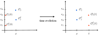
Figure 1: The orbit of chiral part of operators in complex plane

We can also derive this late time value of the OTOC using $3d$ TQFT technology Witten:1988hf . As time passes, the operators evolve as depicted in Fig.1. Their orbits are mapped to 3d links made by the corresponding anyons as in Fig.2.

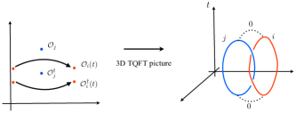
Figure 2: 3d TQFT counterpart. Here, $0$ denotes the identity channel of the conformal blocks.

The relation between 2d CFT and 3d TQFT is given as follows. First, the initial state of 3d TQFT is determined by the sector of conformal block we choose. In this case we choose the identity sector in CFT and in 3d TQFT the pairs of anyons are created from the vacuum. Then, because there is a monodromy in CFT side, there is a link in 3d TQFT side. Finally, corresponding to taking the identity sector at late time, anyons fuse to the vacuum, which means that the final state in the 3d TQFT is given by the pair annihilation of anyons. As a result, we obtain the Hopf link of two Wilson loops. From this observation, we find that the monodromy matrix element is given by the expectation value of the Hopf link divided by the expectation value of two non-linked Wilson loops. Based in results from Witten:1988hf , we find

$$C^{\beta}_{ij}(t)\to{{}_{i}\leavevmode\hbox to41.21pt{\vbox to26.8pt{\text{[drawing]}}}{}_{j}\over{}_{i}\;\leavevmode\hbox to20.72pt{\vbox to20.72pt{\text{[drawing]}}}\;\leavevmode\hbox to23.55pt{\vbox to23.55pt{\text{[drawing]}}}\;{}_{j}}\equiv{1\over d_{i}d_{j}}{S^{*}_{ij}\over S_{00}}.$$ (9)

This exactly matches with the r.h.s of (8) and naturally explains why this combination appears in late time OTOC. If we apply this formula to the Ising model CFT, we reproduce exactly the results from the explicit calculation of monodromy in Appendix B of Roberts:2014ifa .

Let us finally mention that the above late time value, known as monodromy scalar, has been proposed as a measure of non-abelian anyons in interferometry experiments Bonderson . It would be interesting to explore this connection as a possible experimental measure of quantum chaos.

III Purity and quantum dimension

Now, we turn our attention to entanglement. We are interested in a local quench setup where a state is excited by a local operator. More precisely, we take a pure state in a 1+1 dimensional CFT and divide space into two halves $A$ and $\bar{A}$. Then, we insert a local operator ${\cal O}$ with conformal dimension $h=\bar{h}$ into $\bar{A}$ at, say $x=-l$, and study the time evolution of entanglement in the system. In particular, we consider the evolution of the second Rényi entropy; hereafter we refer to this quantity as the purity (strictly speaking the purity corresponds to the logarithm of the square of the reduced density matrix). Using the replica method the purity can be extracted from the canonical 4-point function $\mathcal{G}(z,\bar{z})\equiv\langle\mathcal{O}(0)\mathcal{O}(z,\bar{z})^{\dagger}\mathcal{O}(1)\mathcal{O}^{\dagger}(\infty)\rangle$ and it reads He:2014mwa

$$\Delta S^{(2)}_{A}(z,\bar{z})=-\log\left[|z(1-z)|^{4h}{\cal G}(z,\bar{z})\right]\,,$$ (10)

where the points entering the cross-ratios are expressed in terms of the replica points as $z^{2}_{i}=w_{i}$ where

$$w_{1}=i(\epsilon-it)-l,\ \ w_{2}=-i(\epsilon+it)-l,$$

$$\bar{w}_{1}=-i(\epsilon-it)-l,\ \ \bar{w}_{2}=i(\epsilon+it)-l.$$ (11)

As one takes $\epsilon\to 0$, $\bar{z}\to 0$, meanwhile, $z$ can become either $0$ or $1$ for times earlier or later than $l$ respectively.

In a RCFT given the singularity structure of ${\cal G}$ this implies that $\Delta S^{(2)}_{A}$ vanishes at early times since only the identity channel contributes. Moreover, since early and late times are mapped to each other by the transformation $(z,\bar{z})\to(1-z,\bar{z})$ one finds that the late time purity can be extracted from the fusion matrix element $F_{00}[\mathcal{O}]$. Furthermore, this quantity corresponds to the inverse of the quantum dimension of ${\cal O}$’s conformal family. Hence, at late times we have He:2014mwa ; Caputa:2015tua

$$\Delta S^{(2)}_{A}(t)=\log d_{\cal O}\,.$$ (12)

Observe that the appearance of a constant contribution at late time for $\Delta S^{(2)}_{A}$ is closely related to the singular behavior

$${\cal G}(z,\bar{z})\to d^{-1}_{\mathcal{O}}((1-z)\bar{z})^{-2h}$$ (13)

of the four-point function as $(z,\bar{z})\to(1,0)$. The authors of Asplund:2015eha have argued that in holographic CFTs, where the Ryu-Takayanagi formula Ryu:2006bv is valid, such singularity disappears due to “scrambling of entanglement”. This way, in our setup, the appearance of a the (non-perturbative) quantum dimension at late times is replaced by a divergent logarithmic growth of the Rényi entropy. This fast growth of entanglement is equivalent to the breakdown of the quasi-particle picture that is characteristic of strongly coupled large-c theories. The temperature dependence can be introduced by the standard conformal map (see Caputa:2014eta ) but the logarithmic growth with time at large c is not affected. Below, we will show how this behavior emerges in the “holographic” large-$c$ limit of WZW models.

It is also worth mentioning that the $\log d_{\mathcal{O}}$ increase can be obtained from the topological entanglement entropy wen2 if one of the regions contains an anyonic excitation Dong:2008ft . At first sight the late time purity and the OTOC are rather similar objects i.e. both are captured by the vacuum conformal block. Naively, one would expect to be able to use them interchangeably as indicators of quantum chaos, or even to diagnose whether a CFT has a holographic dual. This is in fact not the case and below we present an example where the purity displays the behavior expected from a holographic theory, while the OTOC doesn’t.

IV On purity and OTOC in $SU(N)_{k}$ WZW

In this section we consider a WZW model with affine Lie algebra $SU(N)_{k}$. Just as the quantum dimension, the late time value OTOC is invariant under level-rank duality, hence, the following discussion is valid for $SU(k)_{N}$ as well. Knowing the modular S-matrix of the model, using (9) we could compute directly the late time OTOC. Here we follow a direct approach instead, both to illustrate the underlying mechanisms and as a consistency check. We focus on the 4-point function of operators $g^{\alpha}_{\beta}(z_{i},\bar{z}_{i})$ (and their conjugates) in the fundamental representation $\alpha=\{1,0,...0\}$ that have conformal dimension

$$h=\bar{h}={N^{2}-1\over 2N\kappa}.$$ (14)

where $\kappa=N+k$. The general correlator that we employ is

$$\langle g^{\alpha_{1}}_{\beta_{1}}(z_{1},\bar{z}_{1})(g^{-1})^{\beta_{2}}_{\alpha_{2}}(z_{2},\bar{z}_{2})g^{\alpha_{3}}_{\beta_{3}}(z_{3},\bar{z}_{3})(g^{-1})^{\beta_{4}}_{\alpha_{4}}(z_{4},\bar{z}_{4})\rangle$$

$$\equiv{1\over|z_{12}|^{4h}|z_{34}|^{4h}}|z|^{4h}\mathcal{G}(z,\bar{z}).$$ (15)

Recall that we characterized OTOCs by the function $f(z,\bar{z})$ which is related to $\mathcal{G}(z,\bar{z})$ via $f(z,\bar{z})=|z|^{2h}\mathcal{G}(z,\bar{z})$. To apply the above correlator in our OTOC we set $\alpha_{1}=\alpha_{2}$, $\beta_{1}=\beta_{2}$ and $\alpha_{3}=\alpha_{4}$ with $\beta_{3}=\beta_{4}$. On the other hand, for the purity all the $\alpha$s (and $\beta$s) and must be equal.

The general 4-point functions (IV) are well known solutions of the Knizhnik-Zamolodchikov equations Knizhnik:1984nr . The canonical correlator can be expanded in terms of affine conformal blocks

$$\mathcal{G}(z,\bar{z})=\sum_{i,j}I_{i}\bar{I}_{j}\sum_{n}X_{nn}\mathcal{F}^{(n)}_{i}(z)\mathcal{F}^{(n)}_{j}(\bar{z}),$$ (16)

with $i,j,n\in\{1,2\}$ and $SU(N)$ factors $I_{1}=\delta^{\alpha_{2}}_{\alpha_{1}}\delta^{\alpha_{4}}_{\alpha_{3}}$, $I_{2}=\delta^{\alpha_{4}}_{\alpha_{1}}\delta^{\alpha_{2}}_{\alpha_{3}}$. In our arguments we will only use $X_{11}=1$, more details can be found in DiF .

Let us compute the purity first. In order to extract the late time value, we apply the fusion transformation that mixes conformal blocks

$${\cal G}(1-z,\bar{z})=\sum_{i,j}I_{i}\bar{I}_{j}\sum_{n,m}X_{nn}c_{nm}\mathcal{F}^{(m)}_{3-i}(z)\mathcal{F}^{(n)}_{j}(\bar{z})\,,$$ (17)

where the relevant coefficient is

$$c_{11}=N{{\Gamma}(N/\kappa){\Gamma}(-N/\kappa)\over{\Gamma}(1/\kappa){\Gamma}(-1/\kappa)}=[N]^{-1}=d^{-1}_{g},$$ (18)

with $d_{g}$ being the quantum dimension for the fundamental representation, where the quantum numbers are defined as

$$[x]={q^{x/2}-q^{-x/2}\over q^{1/2}-q^{-1/2}}\qquad q=e^{-{2\pi i\over N+k}}\,.$$ (19)

Taking the limit of the conformal blocks for $(z,\bar{z})\to(1,0)$ (see App.A) leaves us with the log of the quantum dimension multiplied by the appropriate singularity such that we get the $\log\,[N]$ at late times. It is also interesting to see that even though the four-point correlator is expanded in terms of the affine conformal blocks, that are sums of the Virasoro blocks, the relevant constant is still hidden in the vacuum block. Moreover, from the definition, we have $[N]=[k]$ which is in fact the consequence of the level-rank duality for quantum dimensions inherited by the purity.

Now, let us study the OTOC. Extracting the monodromy around $z=1$ brings us to

$$f(z,\bar{z})=e^{-2\pi i(h_{\theta}-2h)}\sum_{i,j}I_{i}\bar{I}_{j}\sum_{n,m}X_{nn}B_{nm}f^{(m)}_{i}(z)f^{(n)}_{j}(\bar{z}).$$ (20)

where $B_{nm}$ are the monodromy matrix elements of the solutions of the hypergeometric equation (see e.g. Erdelyi ). Taking the limit of $(z,\bar{z})\to(0,0)$ leaves only the terms from $f^{(1)}_{1}$ and we are left with the overall exponent prefactor and the coefficient $B_{11}$ given by

$$B_{11}=1-2ie^{-i\pi(1-{N\over\kappa})}{\sin^{2}({\pi\over\kappa})\over\sin(\pi(1-{N\over\kappa}))}.$$ (21)

After some algebra, and expressing the answer in terms of quantum numbers we find that at late times

$$C^{\beta}_{ij}(t)\to e^{-2\pi i(h_{\theta}-2h)}B_{11}=q^{{1\over N}+{1\over 2}}{\left(q^{-{N+2\over 2}}+[N-1]\right)\over[N]}.$$ (22)

We can compare this answer with our RCFT result Eq. (3). Indeed, the S-matrix element for the present example has been computed in Dong:2008ft and it reads

$${S^{*}_{\alpha\alpha}\over S_{00}}=q^{{1\over N}+{1\over 2}}\left(q^{-{N+2\over 2}}+[N-1]\right)[N]\,,$$ (23)

and inserting $d_{i}=d_{j}=[N]$ beautifully matches (3). For example, for the $SU(2)_{k}$ model, the late time OTO (22) reduces to

$$C^{\beta}_{ij}(t)\to\cos\left({2\pi\over k+2}\right)\cos^{-1}\left({\pi\over k+2}\right)\,,$$ (24)

which can be extracted from the explicit form of the $SU(2)_{k}$ modular S-matrix

$$S_{ij}=\sqrt{{2\over 2+k}}\sin\left({(i+1)(j+1)\pi\over k+2}\right)\,,$$ (25)

by setting $i=j=1$. Note that, in general, the elements of the modular S-matrix can be complex (except the first row that are related to quantum dimensions which are real).

Summarizing, we have shown that late time values of the purity and OTOC are given in terms of the quantum dimensions as well as the modular S-matrix. It is interesting that, in RCFTs, OTOCs give us the access to the entire modular S-matrix whereas Rényi entropies only to the first row $S_{0i}$. It is also interesting to consider the classical limit ($k\to\infty$) of WZW models where the purity becomes the log of the dimension of the fundamental, and the OTOC equals one.

V OTOC and purity in the large-c limit

Finally, it is interesting to compare the behavior of the purity and the OTOC in the large-$c$ limit. In the $SU(N)_{k}$ WZW the central charge is given by

$$c={k(N^{2}-1)\over k+N}\,.$$ (26)

By introducing the ’t Hooft coupling constant

$$\lambda={N\over k}\,,$$ (27)

we can define a ’t Hooft limit of large central charge with the coupling fixed (weak or strong). The four-point correlator has been analyzed in detail in this limit by Kiritsis:2010xc and we apply their analysis in our context. For $c\to\infty$, the 4-point correlator becomes (see App A) (Note that here, unlike in Roberts:2014ifa , all our operators are light: $h/c\to 0$ as $c\to\infty$). Using this correlator, one can see that for a large central charge the singularities leading to the quantum dimension are absent, which leads to a logarithmic growth of the purity

$$\Delta S^{(2)}_{A}(t)\simeq 2h\log\left({2t\over\epsilon}\right)-\log(2).$$ (28)

This behavior comes from discarding terms proportional to ${1\over\sqrt{c}}$. However, if we include such corrections, then the late time answer becomes the logarithm of the quantum dimension in the large-$c$ limit. It is illustrative to verify this in the strong coupling regime, where $h=1/2$ and the correlator (see App A) can be computed by approximating the operators $g^{\alpha}_{\beta}(z_{i},\bar{z}_{i})\simeq{1\over k}\sum^{k}_{i=1}\psi^{\alpha}(z_{i})\bar{\psi}^{\beta}(\bar{z}_{i})$ with complex fermions. In this limit we have

$$\mathcal{G}(z,\bar{z})\simeq{I_{1}\bar{I}_{1}\over|z|^{2}}+{I_{2}\bar{I}_{2}\over|1-z|^{2}}+\sqrt{{\lambda\over c}}\left({I_{1}\bar{I}_{2}\over z(1-\bar{z})}+{I_{2}\bar{I}_{1}\over(1-z)\bar{z}}\right).$$ (29)

Using (10), it is clear that neglecting the last two terms in the above expression leads to the logarithmic growth of the purity in the large-c limit, which is sometimes known as scrambling of entanglement. Another way to look at this order of limits issue is that, at strong coupling, the time scale at which the purity reaches the $\log d_{O}$ can be estimated as $t-l\simeq{c^{1/4}\over 2\lambda^{1/4}}\epsilon$. If we then take the large-c limit first (like in holography), we will not reach the finite constant and we are left with the logarithmic growth with time (see also discussion in Caputa:2014vaa ).

On the other hand, the late time value of the OTOC comes from the first term in (29) (irrespectively of the weak or strong coupling) and in $f(z,\bar{z})$ it is simply 1. For different operators $\alpha_{1}=\alpha_{2}\neq\alpha_{3}=\alpha_{4}$ only $I_{2}$ vanishes so the result remains the same. Thus, OTOC is a good indicator of integrability even when entanglement scrambles.

VI Conclusion

We have shown that OTOC in RCFTs approach to a universal constant at late times which is completely determined in terms of the modular S-matrix of the theory. Moreover, we have pointed out that this quantity is potentially observable in experimental set-ups. We provided a non-trivial example in the integrable $SU(N)_{k}$ WZW model. We also argued in this setup, that in the large-$c$ limit the purity displays the logarithmic growth characteristic of holographic models, but the OTOCs remain constant, as a good measure of quantum chaos should since the theory is far from chaotic. It would be interesting to understand how chaos and scrambling are related and emerge in large-c CFT with holographic duals. Extending our work to operators in higher representations, non-rational CFTs and (non)integrable theories in higher dimensions might shed more light on these issues.

.1 Appendix A: 4-Point function in $SU(N)_{k}$ WZW

From KZ equations one can derive the canonical four-point function that is written in terms of the cross-ratios and the dimensions $h={N^{2}-1\over 2N(k+N)}$ and $h_{\theta}={N\over N+k}$. More precisely, the affine conformal blocks are expressed as

$${\cal F}^{(1)}_{1}(z) = z^{-2h}(1-z)^{h_{\theta}-2h}u_{1}(z)$$

$${\cal F}^{(2)}_{1}(z) = z^{-2h}(1-z)^{h_{\theta}-2h}u_{2}(z)$$

$${\cal F}^{(1)}_{2}(z) = {1\over k}z^{1-2h}(1-z)^{h_{\theta}-2h}\tilde{u}_{1}(z)$$

$${\cal F}^{(2)}_{2}(z) = -Nz^{1-2h}(1-z)^{h_{\theta}-2h}\tilde{u}_{2}(z)$$

with $u(z)_{i}$ and $\tilde{u}_{i}(z)$ being the standard solutions of the hypergeometric equation $u_{1}(z)=\,_{2}F_{1}(a,b,c;z)$ and $u_{2}(z)=z^{1-c}\,_{2}F_{1}(a-c+1,b-c+1,2-c;z),$ where $u_{1}$ and $u_{2}$ parametrized by $a={1\over\kappa}$, $b=-{1\over\kappa}$ and $c=1-{N\over\kappa}$ such that $1-c={N\over\kappa}=h_{\theta}$, and $\tilde{u}_{1}$ and $\tilde{u}_{2}$ of $a=1+{1\over\kappa}$, $b=1-{1\over\kappa}$ and $c=2-{N\over\kappa}$ such that $1-c={N\over\kappa}-1=h_{\theta}-1$. The monodromy of the conformal blocks under the loop that encircles $z=1$ is a combination of the contribution from the pre-factors as well as the monodromy of the hypergeometric functions (see Erdelyi ).

The function ${\cal G}(z,\bar{z})$ in Eq. (16) admits the large-$c$ expansion given by

$${\cal G}(z,\bar{z}) \simeq {I_{1}\bar{I}_{1}\over|z|^{4h}}+{I_{2}\bar{I}_{2}\over|1-z|^{4h}}$$

$$+ {\lambda\over\sqrt{c(1+\lambda)}}\Bigg{[}\Big{(}\gamma(z,\bar{z})\bar{I}_{1}I_{2}+\text{c.c.}\Big{)}\Bigg{]},$$

where

$$\gamma(z,\bar{z})={\,{}_{2}F_{1}\left(1,1,{2+\lambda\over 1+\lambda};z\right)\over\bar{z}^{2h}z^{2h-1}}-{\,{}_{2}F_{1}\left({\lambda\over 1+\lambda},{\lambda\over 1+\lambda},{1+2\lambda\over 1+\lambda};\bar{z}\right)\over\lambda(1-z)^{2h}},$$

with $2h=\lambda/(1+\lambda)$. Notice that around $(z,\bar{z})\approx(1,0)$

$$\gamma(z,\bar{z})\approx\left({\pi\over 1+\lambda}\right){\csc\left({\lambda\over 1+\lambda}\right)\over\bar{z}^{2h}(1-z)^{2h}}\,.$$

Plugging the above expression into ${\cal G}$ and afterwards in (10), one finds a constant contribution to the late time purity; this constant duly corresponds to the logarithm of the first term in the large-c expansion of the quantum dimension.

.2 Appendix B: Liouville theory

It is also interesting to “naively” apply our formula for late time value of OTO in a (non-rational) Liouville 2d CFT with central charge $c=1+6Q^{2}$. From the explicit form of the analog of the S-matrix Zamolodchikov:2001ah (see also Jackson:2014nla ; McGough:2013gka ), the quantum dimension of a non-degenerate operator with weight $\Delta_{p}=p^{2}+{1\over 4}Q^{2}$ reads, $d_{p}=\sinh\left(\pi pb\right)\sinh\left(\pi pb^{-1}\right)$. Moreover, the S-matrix element between two such non-degenerate operators is given by ${\cal S}_{p}^{\,q}=\sqrt{2}\cos\left(\pi pq\right)$. Plugging these into (9) yields at large-c

$$C_{pq}^{\,\beta}(t)\sim\Lambda_{p,q}\,c\,e^{-\pi\left(p+q\right)\sqrt{{c\over 6}}}\,,$$

where $\Lambda_{p,q}$ is a constant that depends on $p$ and $q$. Observe that the above expression is damped exponentially as we increase the central charge in contrast with the RCFT case.

References

- (1) P. Calabrese and J. L. Cardy, “Entanglement entropy and quantum field theory,” J. Stat. Mech. 0406, P06002 (2004), C. Holzhey, F. Larsen and F. Wilczek, “Geometric and renormalized entropy in conformal field theory,” Nucl. Phys. B 424 (1994) 443
- (2) A. Larkin and Y. Ovchinnikov, “Quasiclassical method in the theory of superconductivity”, J. Exp. Theor. Phys. 28, 1200 (1969).
- (3) A. Kitaev. Hidden correlations in the Hawking radiation and thermal noise. - 2014. Talk given at the Fundamental Physics Prize Symposium, Nov. 10.
- (4) D. A. Roberts and D. Stanford, “Two-dimensional conformal field theory and the butterfly effect,” Phys. Rev. Lett. 115, no. 13, 131603 (2015)
- (5) D. A. Roberts, D. Stanford and L. Susskind, “Localized shocks,” JHEP 1503, 051 (2015)
- (6) J. Maldacena, S. H. Shenker and D. Stanford, “A bound on chaos,” arXiv:1503.01409 [hep-th].
- (7) A. L. Fitzpatrick and J. Kaplan, “A Quantum Correction To Chaos,” arXiv:1601.06164 [hep-th].
- (8) M. Nozaki, T. Numasawa and T. Takayanagi, “Quantum Entanglement of Local Operators in Conformal Field Theories,” Phys. Rev. Lett. 112, 111602 (2014)
- (9) S. He, T. Numasawa, T. Takayanagi and K. Watanabe, “Quantum dimension as entanglement entropy in two dimensional conformal field theories,” Phys. Rev. D 90, no. 4, 041701 (2014) doi:10.1103/PhysRevD.90.041701 [arXiv:1403.0702 [hep-th]].
- (10) P. Caputa and A. Veliz-Osorio, “Entanglement constant for conformal families,” Phys. Rev. D 92, no. 6, 065010 (2015)
- (11) P. Caputa and M. M. Rams, “Quantum dimensions from local operator excitations in the Ising model,” arXiv:1609.02428 [cond-mat.str-el].
- (12) S. Ryu and T. Takayanagi, “Holographic derivation of entanglement entropy from AdS/CFT,” Phys. Rev. Lett. 96 (2006) 181602
- (13) P. Caputa, M. Nozaki and T. Takayanagi, “Entanglement of local operators in large-N conformal field theories,” PTEP 2014, 093B06 (2014)
- (14) C. T. Asplund, A. Bernamonti, F. Galli and T. Hartman, “Entanglement Scrambling in 2d Conformal Field Theory,” JHEP 1509, 110 (2015) [arXiv:1506.03772 [hep-th]].
- (15) S. H. Shenker and D. Stanford, “Black holes and the butterfly effect,” JHEP 1403, 067 (2014)
- (16) P. Caputa, J. Simon, A. Stikonas and T. Takayanagi, “Quantum Entanglement of Localized Excited States at Finite Temperature,” JHEP 1501, 102 (2015)
- (17) P. Caputa, J. Simon, A. Stikonas, T. Takayanagi and K. Watanabe, “Scrambling time from local perturbations of the eternal BTZ black hole,” JHEP 1508, 011 (2015)
- (18) The relation between scrambling and OTO correlators was also demonstrated in Hosur:2015ylk but the connection with entanglement scrambling Asplund:2015eha used here is not clear to us at this moment
- (19) A. L. Fitzpatrick, J. Kaplan and M. T. Walters, “Universality of Long-Distance AdS Physics from the CFT Bootstrap,” JHEP 1408, 145 (2014)
- (20) G. W. Moore and N. Seiberg, “Naturality in Conformal Field Theory,” Nucl. Phys. B 313, 16 (1989). G. W. Moore and N. Seiberg, “Polynomial Equations for Rational Conformal Field Theories,” Phys. Lett. B 212, 451 (1988).
- (21) E. Witten, “Quantum Field Theory and the Jones Polynomial,” Commun. Math. Phys. 121, 351 (1989).
- (22) P. Bonderson, K. Shtengel and J. K. Slingerland, ”Probing Non-Abelian Statistics with Quasiparticle Interferometry,” Phys. Rev. Lett. 97.016401, 2006.
- (23) A. Kitaev and J. Preskill, “Topological entanglement entropy,” Phys. Rev. Lett. 96, 110404 (2006) M. Levin and X. G. Wen, Phys. Rev. Lett. 96, 110405 (2006)
- (24) S. Dong, E. Fradkin, R. G. Leigh and S. Nowling, “Topological Entanglement Entropy in Chern-Simons Theories and Quantum Hall Fluids,” JHEP 0805, 016 (2008)
- (25) V. G. Knizhnik and A. B. Zamolodchikov, “Current Algebra and Wess-Zumino Model in Two-Dimensions,” Nucl. Phys. B 247, 83 (1984).
- (26) P. Di Francesco, P. Mathieu, D. Senechal (1997) ”Conformal field theory”
- (27) P. Hosur, X. L. Qi, D. A. Roberts and B. Yoshida, “Chaos in quantum channels,” arXiv:1511.04021 [hep-th].
- (28) E. Kiritsis and V. Niarchos, “Large-N limits of 2d CFTs, Quivers and duals,” JHEP 1104 (2011) 113
- (29) Erdelyi, A., W. Magnus, F. Oberhettinger and F.G. Tricomi: ”Higher transcendental functions, Vol.1”, McGraw-Hill, New York, 1953. (see page 93)
- (30) A. B. Zamolodchikov and A. B. Zamolodchikov, “Liouville field theory on a pseudosphere,” hep-th/0101152.
- (31) Y. Gu and X. L. Qi, “Fractional Statistics and the Butterfly Effect,” JHEP 1608, 129 (2016) [arXiv:1602.06543 [hep-th]].
- (32) S. Jackson, L. McGough and H. Verlinde, “Conformal Bootstrap, Universality and Gravitational Scattering,” Nucl. Phys. B 901, 382 (2015)
- (33) L. McGough and H. Verlinde, “Bekenstein-Hawking Entropy as Topological Entanglement Entropy,” JHEP 1311, 208 (2013)