Uniform Hypergraph Partitioning:
Provable Tensor Methods and Sampling Techniques

Abstract

In a series of recent works, we have generalised the consistency results in the stochastic block model literature to the case of uniform and non-uniform hypergraphs. The present paper continues the same line of study, where we focus on partitioning weighted uniform hypergraphs—a problem often encountered in computer vision. This work is motivated by two issues that arise when a hypergraph partitioning approach is used to tackle computer vision problems:
(i) The uniform hypergraphs constructed for higher-order learning contain all edges, but most have negligible weights. Thus, the adjacency tensor is nearly sparse, and yet, not binary.
(ii) A more serious concern is that standard partitioning algorithms need to compute all edge weights, which is computationally expensive for hypergraphs. This is usually resolved in practice by merging the clustering algorithm with a tensor sampling strategy—an approach that is yet to be analysed rigorously.

We build on our earlier work on partitioning dense unweighted uniform hypergraphs (Ghoshdastidar and Dukkipati, ICML, 2015), and address the aforementioned issues by proposing provable and efficient partitioning algorithms. Our analysis justifies the empirical success of practical sampling techniques. We also complement our theoretical findings by elaborate empirical comparison of various hypergraph partitioning schemes.

Keywords: Hypergraph partitioning, planted model, spectral method, tensors, sampling, subspace clustering

1 Introduction

Over several decades, the study of networks or graphs has played a key role in analysing relational data or pairwise interactions among entities. While networks often arise naturally in social or biological contexts, there are several machine learning algorithms that construct graphs to capture the similarity among data instances. A classic example of this approach is the spectral clustering algorithm of Shi and Malik (2000) that performs image segmentation by partitioning a graph constructed on the image pixels, where the weighted edges capture the visual similarity of the pixels. In general, graph partitioning and related problems are quite popular in unsupervised learning (Ng et al., 2002; Cour et al., 2007), dimensionality reduction (Zhao and Liu, 2007), semi-supervised learning (Belkin et al., 2004) as well as transductive inference (Wang et al., 2008). In spite of the versatility of the graph based approaches, these methods are often incapable of handling complex networks that involve multi-way interactions. For instance, consider a market transaction database, where each transaction or purchase corresponds to a multi-way connection among commodities involved in the transaction (Guha et al., 1999). Such networks do not conform with a traditional graph structure, and need to be modelled as hypergraphs. Similar multi-way interactions have been considered in the case of molecular interaction networks (Michoel and Nachtergaele, 2012), VLSI circuits (Karypis and Kumar, 2000), tagged social networks (Ghoshal et al., 2009), categorical databases (Gibson et al., 2000), computer vision (Agarwal et al., 2005) among others. In this work, we consider the network clustering problem for hypergraphs, where all the edges are of same cardinality. Uniform hypergraph partitioning finds use in computer vision applications such as subspace clustering (Agarwal et al., 2005; Rota Bulo and Pelillo, 2013), geometric grouping (Govindu, 2005; Chen and Lerman, 2009) or higher-order matching (Duchenne et al., 2011).

Uniform hypergraphs have been in the limelight of theoretical research for more than a century with the problem of hypergraph colorability surfacing in early $20^{th}$ century (Bernstein, 1908) to recent works establishing sharp phase transitions in random hypergraphs (see references in Bapst and Coja-Oghlan, 2015). However, there has been much less interest in studying practical machine learning problems that deal with uniform hypergraphs. For instance, restricting our discussion to the network partitioning, one can immediately notice a sharp contrast in the theoretical understanding of the problem in the context of graph and hypergraphs. Spectral graph partitioning algorithms have been analysed from different perspectives since the works of McSherry (2001) and Ng et al. (2002). The seminal work of Rohe et al. (2011), which studied standard spectral clustering under the stochastic block model, drew the attention of both statisticians and computer scientists, and has led to significant advancements in understanding of when the partitions can be detected, and which algorithms achieve optimal error rates (see Abbe and Sandon, 2016, for the current state of the art). In contrast, a similar line of study in the context of hypergraphs is quite recent (Ghoshdastidar and Dukkipati, 2014; Ghoshdastidar and Dukkipati, 2015b; Ghoshdastidar and Dukkipati, 2017; Florescu and Perkins, 2016).

Florescu and Perkins (2016) recently solved the problem of optimally detecting two equal-sized partitions in a planted unweighted hypergraph governed by a single parameter. On the other hand, the primary focus of our works has been to analyse the consistency of hypergraph partitioning approaches used in practice under a more general planted model. In Ghoshdastidar and Dukkipati (2014), we presented a generic planted model for dense uniform hypergraphs, and analysed the tensor decomposition based clustering algorithm of Govindu (2005) under this model. Subsequently, in Ghoshdastidar and Dukkipati (2015b), we found that a wide class of so-called “higher order” clustering algorithms can be unified by a common framework of tensor trace maximisation, which is quite similar in spirit to the associativity maximisation problem posed in the case of graph partitioning (Shi and Malik, 2000). We further proposed to solve a relaxation of the problem using a simple, spectral scheme that was consistent, and achieved better error rates compared to our previously studied approach. An extension of the whole setting to the case of sparse non-uniform hypergraphs came next on our agenda (Ghoshdastidar and Dukkipati, 2017), and we proved consistency of a spectral approach for non-uniform hypergraph partitioning.

Like graphs, sparsity turns out to be an important characteristics of real-world hypergraphs. While this fact complicates analysis of the algorithms (see Ghoshdastidar and Dukkipati, 2017; Florescu and Perkins, 2016), it definitely provides significant computational relief. For instance, it is easy to realise that for any network clustering scheme, the computational complexity is at least linear in the number of edges. Hence, for a $m$-uniform hypergraph on $n$ vertices, any standard approach should have a $O(n^{m})$ runtime unless the hypergraph is sparse. This is precisely the problem that one encounters in vision applications, where the network is not given a priori, but one constructs a weighted hypergraph using $m$-way similarities among data instances. Thus, one needs to spend $O(n^{m})$ runtime to construct the entire adjacency tensor only to realise at the end that only few edges have significant weights, and will aid the partitioning scheme. This scenario motivates the study in our present work, where we allow the planted hypergraph to have weighted edges, and still be sparse (in the sense that most weights are close to zero). But, at the same time, the non-zero entries are not known a priori, and hence, efficient schemes are required to perform the partitioning by observing only a small subset of the $O(n^{m})$ edge weights.

1.1 Contributions in this Paper

We build on our earlier work. To be precise, we study the approach presented in Ghoshdastidar and Dukkipati (2015b), which solves a relaxation of the tensor trace maximisation (TTM) problem that lies at the heart of a variety of higher order learning methods. On the other hand, the model under consideration is that of sparse planted uniform hypergraph similar to the one studied in Ghoshdastidar and Dukkipati (2017). However, unlike previous works, we do not restrict the edge weights to be binary, but arbitrary random variables lying in the interval $[0,1]$. So, the sparsity parameter in our model reduces the mean edge weights, leading to a large amount of edges with negligibly small weights, and hence, creating computational challenges of identifying significant edges. The planted model is formally described in Section 2, while our spectral approach is briefly recapped in Section 3. It might come as a surprise to many that this work does not make use the wide range of tensor decomposition techniques that have now become standard tools in machine learning. In Section 2, we discuss in detail how our model violates the common structural assumptions used in the tensor literature.

Our first contribution is presented in Section 4, where we analyse the basic TTM approach under the above mentioned planted model for weighted $m$-uniform hypergraphs. We note that in Ghoshdastidar and Dukkipati (2015b), we had studied the problem only in the dense unweighted case, whereas similarity hypergraphs encountered in subspace clustering etc. are weighted and typically have large number of insignificant edges (sparse). Furthermore, we recall that spectral partitioning methods, for graphs or hypergraphs, typically require a final step of distance based clustering. While $k$-means is the practical choice at this stage, theoretical studies even in the block model literature often use alternative schemes that are easy to analyse. Adhering to our goal of studying practical methods, our analysis utilises guarantees of $k$-means algorithm (Ostrovsky et al., 2012) instead of resorting to standard assumptions (Lei and Rinaldo, 2015) or other schemes (Gao et al., 2015). In this general setting, Theorem 2 presents the error rate of the TTM approach under mild restrictions on sparsity. Furthermore, recent results of Florescu and Perkins (2016) for the special case of bi-partitioning suggests that our analysis is nearly optimal. We also show that the performance of this method is similar to the normalised hypergraph cut approach studied in Ghoshdastidar and Dukkipati (2017), and is superior than tensor decomposition based partitioning of Ghoshdastidar and Dukkipati (2014).

The second and key contribution in this paper is the analysis of a sampled variant of the TTM approach given in Section 5. As noted above, any basic partitioning scheme would have a $\Omega(n^{m})$ runtime merely due to the construction of the entire adjacency tensor. We consider a scenario where only $N$ edges are randomly sampled (with replacement) according to some pre-specified distribution. Theorem 9 provides a lower bound on the sample size $N$ so that the sampled variant achieves desired error rate. The proof of this result borrows ideas from matrix sampling techniques (Drineas et al., 2006), but mainly relies on a trick of rephrasing the problem such that matrix Bernstein inequality can be applied. The analysis provides quite striking conclusions. For instance, under a simplified setting, if hypergraph is dense and consists of a constant number of partitions, then it is sufficient to observe only $\Omega(n(\ln n)^{2})$ uniformly sampled edges. For sparse hypergraphs, uniform sampling cannot improve upon the $\Omega(n^{m})$ runtime, but a certain choice of sampling distribution works with only $N=\Omega(n(\ln n)^{2})$. To the best of our knowledge, this is the first work that analyses graph / hypergraph partitioning with sampling, and such sampling rates have not been previously observed in any related tensor problem. Typically, most methods need to observe about $\Omega(n^{m/2})$ entries of the tensor in order to estimate its decomposition (see, for instance, Bhojanapalli and Sanghavi, 2015; Jain and Oh, 2014), whereas we find that much less observations are required for the purpose of clustering. Our analysis also justifies the popularity of the iterative sampling schemes (Chen and Lerman, 2009; Jain and Govindu, 2013) in the higher order clustering literature.

Our final contribution is purely algorithmic. We present an iteratively sampled variant of the TTM algorithm, and conduct an extensive numerical comparison of various methods in the context of both hypergraph partitioning and subspace clustering. Section 6 presents a wide variety of empirical studies that (i) validate our theoretical findings regarding relative merits of TTM over previously studied algorithms, (ii) compare spectral methods to other hypergraph partitioning algorithms, including popular hMETIS tool (Karypis and Kumar, 2000), and (iii) weigh the merits of hypergraph partitioning in subspace clustering applications, including benchmark problems. Such empirical studies, though often seen in the subspace clustering works, was long overdue in the higher order learning literature. We also hope that the implementations will help standardising subsequent studies in this direction.

We also note here that to achieve clarity of presentation, the sections only contain the outline of proofs of the main results. The proofs of the intermediate lemmas and corollaries are given in the appendix that follows after the concluding section (Section 7).

1.2 Notations

We conclude this section by stating the standard terminology and notations that we follow in the rest of the paper. We denote tensors in bold faces ($\mathbf{A},\mathbf{B}$ etc.), matrices in capitals ($A,Z$ etc.), while vectors and scalars will be understood from the context. We use Trace$(\cdot)$ to write the sum of diagonal entries of a matrix or tensor, and $\|\cdot\|_{2}$ for Euclidean norm for vector and the spectral norm for matrix. For a matrix, say $A$, $A_{i\cdot}$ (or $A_{\cdot i}$) represents its $i^{th}$ row (column), $\|A\|_{F}$ denotes its Frobenius norm, and $\lambda_{i}(A)$ is the $i^{th}$ largest eigenvalue or singular value of $A$ (depending on context). We also use the standard $O(\cdot)$, $o(\cdot)$ and $\Omega(\cdot)$ notations, where, unless specified otherwise, the corresponding quantities are viewed as function of $n$. In addition, $\mathds{1}\{\cdot\}$ is the indicator function, and $\ln(\cdot)$ is natural logarithm.

Moreover, the results in this paper consider two sources of randomness—the random model for hypergraph, and random sampling of edges (or tensor entries). We make this distinction in the notation for expectation, variance and probability by specifying the underlying measure. For instance, $\mathsf{E}_{H}[\cdot]$ is expectation with respect to distribution of the planted model, and $\mathsf{E}_{S|H}[\cdot]$ is the expectation over sampling distribution conditioned on a given random hypergraph. Similar subscripts have been used for probability, $\mathsf{P}(\cdot)$, and variance, $\mathsf{Var}(\cdot)$. Note that for a matrix $A$, $\mathsf{E}_{H}[A]$ refers to its entry-wise expectation.

2 Formal Description of the Problems

We consider the following random model. Let $\mathcal{V}=\{1,2,\ldots n\}$ be a set of $n$ nodes, and $\psi:\{1,2,\ldots,n\}\to\{1,2,\ldots,k\}$ be a (hidden) partition of the nodes into $k$ classes. For a node $i$, we denote its class by $\psi_{i}$. For a fixed integer $m\geq 2$, let $\alpha_{n}\in[0,1]$, and $\mathbf{B}\in[0,1]^{k\times k\times\ldots\times k}$ be a symmetric $k$-dimensional tensor of order $m$. Let $\mathcal{E}$ be the collection of all subsets of $\mathcal{V}$ of size $m$. A random weighted $m$-uniform hypergraph $(\mathcal{V},\mathcal{E},w)$ is generated through the random function $w:\mathcal{E}\to[0,1]$ such that

$$\mathsf{E}[w(\{i_{1},i_{2},\ldots,i_{m}\})]=\alpha_{n}\mathbf{B}_{\psi_{i_{1}}\psi_{i_{2}}\ldots\psi_{i_{m}}}$$ (1)

for all $e=\{i_{1},i_{2},\ldots,i_{m}\}\in\mathcal{E}$, and the collection of random variables $(w(e))_{e\in\mathcal{E}}$ are mutually independent. For convenience, we henceforth write $w_{e}$ instead of $w(e)$. The above model extends the planted partition model for graphs (McSherry, 2001), and is a weighted variant of the planted uniform hypergraph model studied in our earlier works. In particular, if $\alpha_{n}=1$ and $w_{e}$ are independent Bernoulli random variables satisfying (1), then one retrieves the model of Ghoshdastidar and Dukkipati (2014). We present our results for weighted hypergraphs due to their extensive use in computer vision (e.g., Agarwal et al., 2005). Note that the edge distributions are governed by $\mathbf{B}$ and $\psi$, and hence, depend only on the class membership. In addition, $\alpha_{n}$ accounts for sparsity of the hypergraph. Under this setting, the objective of a hypergraph partitioning algorithm is to estimate $\psi$ from a given random instance of the $m$-uniform hypergraph $(\mathcal{V},\mathcal{E},w)$. Throughout this paper, we are interested in bounding the error incurred by a partitioning algorithm, defined as a multi-class 0-1 loss

$$\mathsf{Err}(\psi,\psi^{\prime})=\min_{\sigma}\sum_{i=1}^{n}\mathds{1}\{\psi_{i}\neq\sigma(\psi_{i}^{\prime})\}\;,$$ (2)

where $\psi$ and $\psi^{\prime}$ denote the true and the estimated partitions, respectively, and $\sigma$ is any permutation on $\{1,2,\ldots,k\}$. Note that we also allow number of classes $k$ to grow with $n$.

The first part of the paper builds on the tensor trace maximisation method of Ghoshdastidar and Dukkipati (2015b), and we prove statistical consistency of TTM under the above sparse planted partition model. To be precise, we show that under certain conditions on $\alpha_{n}$ and $\mathbf{B}$, this method achieves $\mathsf{Err}(\psi,\psi^{\prime})=o(n)$. In the block model terminology (Mossel et al., 2013), this statement implies that the algorithm is weakly consistent. Furthermore, if the hypergraph is dense $(\alpha_{n}=1)$, then we show that TTM can exactly recover the partitions, i.e., $\mathsf{Err}(\psi,\psi^{\prime})=o(1)$, and hence, exhibits strong consistency properties. From the recent work of Florescu and Perkins (2016), which studies the special case of bi-partitioning, one can see that our restrictions on $\alpha_{n}$ are nearly optimal (upto a difference of $(\ln n)^{2}$) in the case of bi-partitioning as one cannot detect partitions for sparser hypergraphs.

Next we study partitioning algorithms that compute weights of only $N$ out of $\binom{n}{m}$ edges. For the theoretical analysis, we assume that there is a known probability mass function $(p_{e})_{e\in\mathcal{E}}$, and $N$ edges are sampled with replacement from this distribution. We are interested in finding the minimum $N$ that guarantees weak consistency of the sampled TTM approach. We focus on two sampling distributions: (i) uniform sampling, and (ii) weighted sampling where $p_{e}\propto w_{e}$. Surprisingly, we see that if $\alpha_{n}=1$ (dense case), only $N=\Omega(nk^{2m-1}(\ln n)^{2})$ edges are sufficient for either sampling strategies. This leads to a drastic improvement in runtime, particularly if $k=O(1)$, and even in general, since typically $k$ grows much slower than $n$. However, if $\alpha_{n}$ decays rapidly with $n$, then more samples are needed for the case of uniform sampling, whereas the alternative strategy still works for $N=\Omega(nk^{2m-1}(\ln n)^{2})$. A comparison with tensor literature is not very meaningful, but known methods of the latter field typically need to observe $\Omega(n^{m/2})$ tensor entries (Bhojanapalli and Sanghavi, 2015). In practice, however, computing the weighted sampling distribution requires a single pass over the adjacency tensor, which still takes $O(n^{m})$ time. But, we argue that practical iterative schemes essentially approximate this distribution without observing the entire tensor.

2.1 A Look at Alternative (or Possible) Approaches

This may be a good time to reflect on the history of both hypergraphs and tensors with the focus of understanding the theoretical or practical tools that either fields provide for the planted uniform hypergraph problem. Before proceeding further, it will be helpful to take a look at the adjacency tensor of the random (planted) hypergraph.

Let $\mathbf{A}\in[0,1]^{n\times n\times\ldots\times n}$ be the symmetric adjacency tensor of order $m$. Let $Z\in\{0,1\}^{n\times k}$ be the assignment matrix of the latent partition $\psi$, i.e., $Z_{ij}=\mathds{1}\{\psi_{i}=j\}$. Then we have

$$\mathbf{A}_{i_{1}i_{2}\ldots i_{m}}=\left\{\begin{array}[]{ll}\sum\limits_{j_{1},..,j_{m}=1}^{k}\alpha_{n}\mathbf{B}_{j_{1}j_{2}\ldots j_{m}}Z_{i_{1}j_{1}}\ldots Z_{i_{m}j_{m}}+\mathbf{E}_{i_{1}i_{2}\ldots i_{m}}&\text{for distinct }i_{1},\ldots,i_{m}\\ 0&\text{otherwise,}\end{array}\right.$$ (3)

where $\mathbf{E}$ is a symmetric random tensor with zero mean entries. For ease of understanding, one may ignore the $O(n^{m-1})$ entries of $\mathbf{A}$ with repeated indices to write

$$\mathbf{A}\approx\alpha_{n}(\mathbf{B}\times_{1}Z\times_{2}Z\times_{3}\ldots\times_{m}Z)+\text{noise term},$$ (4)

where $\times_{l}$ denotes the mode-$l$ product between a tensor and a matrix (De Lathauwer et al., 2000). The basic problem is to detect $Z$ from a given $\mathbf{A}$.

The above form is quite similar to the representation of a tensor in terms of its higher order singular value decomposition or HOSVD (De Lathauwer et al., 2000). In fact, it shows that the random adjacency tensor has a multilinear rank approximately $k\ll n$, and clearly suggests that the partitioning problem should be viewed as a tensor decomposition problem. This hint was quickly picked up by Govindu (2005), who proposed a spectral approach for higher order clustering based on HOSVD. Long after this work, tensor methods have gained significant popularity in machine learning in recent years. However, only few works (Bhaskara et al., 2014; Anandkumar et al., 2015) consider decomposition of tensor into asymmetric rank-one terms, while most of the machine learning literature (Anandkumar et al., 2014; Ma et al., 2016) consider decomposition into symmetric rank-one terms. To be more precise, (3) suggests that

$$\mathbf{A}\approx\sum_{j_{1},\ldots,j_{m}=1}^{k}\alpha_{n}\mathbf{B}_{j_{1}j_{2}\ldots j_{m}}Z_{\cdot j_{1}}\otimes Z_{\cdot j_{2}}\otimes\ldots\otimes Z_{\cdot j_{m}}+\text{noise},$$

where $\otimes$ is the tensor outer product. Clearly the $k^{m}$ rank-one terms are asymmetric. It is well known that such a tensor can be represented by a symmetric outer product decomposition only in an algebraically closed field (Comon et al., 2008), i.e., one can write as sum of symmetric rank-one terms, but the vectors in the decomposition are not guaranteed to be real, and hence, will be of little use. We note that though the works of Bhaskara et al. (2014) and Anandkumar et al. (2015) are applicable, their incoherence assumption is clearly violated in the present context where the same vectors appear in all $m$ modes, and with multiplicity greater than one.

Under simpler settings such as the one described later in Section 4.1, one can express $\mathbf{A}$ as a sum of $(k+1)$ symmetric terms of the form

$$\mathbf{A}\approx\sum_{j=1}^{k}\alpha_{n}pZ_{\cdot j}^{\otimes m}+\alpha_{n}qv^{\otimes m}+\text{noise},$$ (5)

where $v=\sum_{j}Z_{\cdot j}$ and $p,q$ are parameters defining $\mathbf{B}$. Such tensors, which have a finite symmetric CP-rank (Candecomp/Parafac), have been extensively studied in machine learning. For a single rank-one term, optimal detection rates are known under Gaussian noise (Richard and Montanari, 2014). Though there is no distributional assumption on the noise term in our case, (1) does imply that the variance of the noise is smaller than the signal, i.e., specialised to this setting, our model lies in the detection region. Unfortunately, single rank-one term occurs for $k=1$, which does not correspond to any meaningful hypergraph problem, and hence, such results are of little use in our case. It may seem that the case of $k\geq 2$ can still be tackled using tensor power iteration based approaches (Anandkumar et al., 2014, 2015), but the necessary incoherence criterion is violated even here since $v$ has a significant overlap with each $Z_{\cdot j}$. To summarise, it suffices to say that existing guarantees in the tensor literature are not directly applicable for solving (5), but it does not rule out the possibility that a careful analysis of power iterations (Anandkumar et al., 2014) or alternative approaches (Ma et al., 2016) may lead to alternative partitioning techniques. That being said, one should note that (5) is merely a special case of (3), where HOSVD still appears to be the natural answer.

Interestingly, uniform hypergraphs predate the tensor literature, and one may refer to Berge (1984) for early development. Even hypergraph partitioning came into practice (Schweikert and Kernighan, 1979) before tensor decompositions gained popularity. However, initial approaches to hypergraph partitioning in VLSI (Karypis and Kumar, 2000) and database (Gibson et al., 2000) communities relied on clever combination of heuristics with no known performance guarantees. Subsequent works in computer vision (Agarwal et al., 2005) and machine learning (Zhou et al., 2007) proposed spectral solutions for the problem. Such approaches are more amenable for a theoretical analysis. While the analysis in Ghoshdastidar and Dukkipati (2017) and Florescu and Perkins (2016) are somewhat based on the hypergraph cut approach of Zhou et al. (2007), the algorithm studied in this paper is closely related to work of Agarwal et al. (2005). The key idea of such spectral schemes is to reduce the hypergraph into a graph and then apply spectral clustering. Quite surprisingly, we show in this paper that both schemes perform better than HOSVD based partitioning both theoretically (Remark 5) and numerically (Section 6.1). This is counter-intuitive since one would expect significant information loss during the reduction to a graph. A careful look at the algorithm presented in the next section would reveal that this is not the case. While most information in modes $3,\ldots,m$ are lost, one can still estimate $Z$ from the first two modes, which suffices for the purpose of detecting planted partitions. This observation is reinforced by the recent study of Florescu and Perkins (2016), where the authors show that a reduction based spectral approach can optimally detect two partitions all the way down to the limit of identifiability of the partitions.

We conclude this section with a brief mention of the wide variety of other higher order learning methods, which include tensor based clustering algorithms (Shashua et al., 2006; Chen and Lerman, 2009; Arias-Castro et al., 2011; Ochs and Brox, 2012), other unsupervised tensorial learning schemes (Duchenne et al., 2011; Nguyen et al., 2015), as well as related optimisation approaches (Leordeanu and Sminchisescu, 2012; Rota Bulo and Pelillo, 2013; Jain and Govindu, 2013), and can easily be represented as instances of the uniform hypergraph partitioning problem. In Ghoshdastidar and Dukkipati (2015b), we showed that most of the above methods can be unified by a general tensor trace maximisation (TTM) problem. A spectral solution to this problem is analysed in the present paper, and thus, we believe that some of our conclusions can also be extended to these alternative approaches. We also numerically compare with some of these methods in Section 6.

3 Tensor Trace Maximisation (TTM)

In this section, we briefly recap the work in Ghoshdastidar and Dukkipati (2015b) and then present the basic approach that will be later analysed and modified in the remainder of the paper. Let $(\mathcal{V},\mathcal{E},w)$ be a given weighted uniform hypergraph, where $\mathcal{E}$ is the collection of all sets of $m$ vertices, and $w:\mathcal{E}\to[0,1]$ associates a weight with every edge. We consider the problem of partitioning $\mathcal{V}$ into $k$ disjoint sets, $\mathcal{V}_{1},...,\mathcal{V}_{k}$, such that the total weight of edges within each cluster is high, and the partition is ‘balanced’. In the case of graphs, i.e., for $m=2$, the popular heuristic for achieving these two conditions is the normalised cut minimisation problem, or equivalently normalised associativity maximisation problem (Shi and Malik, 2000; von Luxburg, 2007). We extend this approach to uniform hypergraphs.

3.1 TTM Approach and Algorithm

We consider the problem of finding the partition of the vertices that maximises the normalised associativity. This is subsequently formulated in terms of a tensor trace maximisation objective. We define few terms. The degree of any node $v\in\mathcal{V}$ is the total weight of edges on which $v$ is incident, i.e., $\textup{deg}(v)=\sum\limits_{e\in\mathcal{E}:v\in e}w_{e}$. For any collection of nodes $\mathcal{V}_{1}\subseteq\mathcal{V}$, we define its volume as $\textup{vol}(\mathcal{V}_{1})=\sum\limits_{v\in\mathcal{V}_{1}}\textup{deg}(v)$ and its associativity as $\textup{assoc}(\mathcal{V}_{1})=\sum\limits_{e\in\mathcal{E}:e\subset\mathcal{V}_{1}}w_{e}$, which is the total weight of edges contained within $\mathcal{V}_{1}$. The normalised associativity of a partition $\mathcal{V}_{1},...,\mathcal{V}_{k}$ is given as

$$\textup{N-Assoc}(\mathcal{V}_{1},\ldots,\mathcal{V}_{k})=\sum_{i=1}^{k}\frac{\textup{assoc}(\mathcal{V}_{i})}{\textup{vol}(\mathcal{V}_{i})}\;.$$ (6)

Observe that the above definitions coincide with the corresponding terms in graph literature (Shi and Malik, 2000). We now follow the popular goal of finding clusters that maximises the normalised associativity (6). In the case of graphs, it is well known that the problem can be reformulated in terms of the adjacency matrix of the graphs, which results in a matrix trace maximisation problem (von Luxburg, 2007). Furthermore, a spectral relaxation allows one to find an approximate solution for the problem by computing the $k$ dominant eigenvectors of the normalised adjacency matrix. A similar approach is possible in the case of uniform hypergraphs. Let $\mathbf{A}$ be the adjacency tensor (of order $m$), i.e.,

$$\mathbf{A}_{i_{1}i_{2}\ldots i_{m}}=\left\{\begin{array}[]{ll}w_{\{i_{1},i_{2},\ldots,i_{m}\}}&\text{if }i_{1},i_{2},\ldots,i_{m}\text{ are distinct},\\ 0&\text{otherwise}.\end{array}\right.$$ (9)

Define $\beta_{1},...,\beta_{m}\in[0,1]$ with $\sum\limits_{l=1}^{m}\beta_{l}=1$, and $Y^{(1)},\ldots,Y^{(m)}\in\mathbb{R}^{n\times k}$ with $Y_{ij}^{(l)}=\left(\frac{\mathds{1}\{i\in\mathcal{V}_{j}\}}{\textup{vol}(\mathcal{V}_{j})}\right)^{\beta_{l}}$. Then, one can rewrite (6) (see appendix for details) as

$$\textup{N-Assoc}(\mathcal{V}_{1},\ldots,\mathcal{V}_{k})=\frac{1}{m!}\textup{Trace}\left(\mathbf{A}\times_{1}{Y^{(1)}}^{T}\times_{2}{Y^{(2)}}^{T}\times_{3}\ldots\times_{m}{Y^{(m)}}^{T}\right)\;,$$ (10)

where $\times_{l}$ denotes the mode-$l$ product. Thus, for some chosen parameters $\beta_{1},\ldots,\beta_{m}$, one can pose the associativity maximisation problem as a tensor trace maximisation (TTM).

In Ghoshdastidar and Dukkipati (2015b), we showed that the above optimisation has connections with the tensor eigenvalue problem (Lim, 2005) and the tensor diagonalisation problem (Comon, 2001). More interestingly, it also lies at the heart of several higher-order learning algorithms. For instance, $\beta_{1}=\ldots=\beta_{m}=\frac{1}{m}$ results in the method of Shashua et al. (2006), while the same strategy when used with $k=1$ has been used to successively extract clusters (Rota Bulo and Pelillo, 2013; Leordeanu and Sminchisescu, 2012). A similar idea lies in some tensor matching algorithms (Duchenne et al., 2011; Nguyen et al., 2015). Another strategy is to set $\beta_{1}=\beta_{2}=\frac{1}{2}$ and $\beta_{3}=\ldots=\beta_{m}=0$. This squeezes the tensor into a matrix, which allows one to use subsequently graph partitioning tools. Our algorithm described below takes this route, and similar ideas have been previously used (Agarwal et al., 2005; Arias-Castro et al., 2011). This reduction also corresponds to the clique expansion of a hypergraph, where every $m$-way edge is replaced by $\binom{m}{2}$ pairwise edges.

We list our basic spectral approach in Algorithm TTM, and we later study the consistency of TTM and its sampled variants. Note that a spectral relaxation of the problem is a two-fold procedure, where first we construct a matrix from the affinity tensor $\mathbf{A}$, and then relax the problem into a matrix spectral decomposition type objective. This principle is reminiscent of the classical technique for studying spectral properties of hypergraphs (Bolla, 1993), and is closely related to approach of the clustering graph approximations of hypergraphs (Agarwal et al., 2006).

Algorithm TTM : Spectral relaxation of tensor trace maximisation problem

0:  Affinity tensor $\mathbf{A}$ of the $m$-uniform hypergraph $(\mathcal{V},\mathcal{E},w)$, where $|\mathcal{V}|=n$.

1:  Read $\mathbf{A}$, and compute the $n\times n$ matrix $A$ as $A_{ij}=\sum\limits_{i_{3},\ldots,i_{m}=1}^{n}\mathbf{A}_{iji_{3}\ldots i_{m}}$.

2:  Let $D\in\mathbb{R}^{n\times n}$ be diagonal with $D_{ii}=\sum\limits_{j=1}^{n}A_{ij}$, and $L=D^{-1/2}AD^{-1/2}$.

3:  Compute $k$ dominant eigenvectors of $L$, denoted by $X\in\mathbb{R}^{n\times k}$ .

4:  Normalise rows of $X$ to have unit norm, and denote this matrix as $\overline{X}$.

5:  Run $k$-means on the rows of $\overline{X}$.

5:  Partition of $\mathcal{V}$ that correspond to the clusters obtained from $k$-means.

A careful look at computational complexity of the algorithm will be helpful for our discussions in Section 5. To this end, we note that our analysis assumes the use $k$-means approach of Ostrovsky et al. (2012), which has a complexity of $O(k^{2}n+k^{4})$ since the data is embedded in a $k$-dimensional space. Furthermore, Steps 2 to 4 involve only matrix operations with the eigenvector computation being the most expensive operation. One may compute the $k$ dominant eigenvectors using power iterations, which can be done provably in $O(kn^{2}\ln(kn))$ runtime (Boutsidis et al., 2015). However, the computational bottleneck of the algorithm is Step 1, which has complexity of $m^{2}|\mathcal{E}|=O(m^{2}n^{m})$. This is not surprising since any network partitioning method should have have complexity at least linear in the number of edges. But it gets quite challenging in computer vision problems, where one often requires to consider higher order relations, for instance $m=4$ used in Duchenne et al. (2011), $m=5$ in Chen and Lerman (2009) and even $m=8$ in Govindu (2005). The aim of Section 5 is to reduce this complexity to $m^{2}N$ by sampling only $N\ll n^{m}$ edges.

4 Consistency of Algorithm TTM under Planted Partition Model

The first task in our agenda is to analyse the basic TTM approach. This section extends the results in Ghoshdastidar and Dukkipati (2015b) to the the planted partition model for sparse weighted hypergraphs described in Section 2. Recall that our aim is to derive an upper bound on $\mathsf{Err}(\psi,\psi^{\prime})$, where $\psi$ and $\psi^{\prime}$ denote the true and the estimated clusters. Moreover, for the purpose of analysis we assume that the $k$-means step is performed using Lloyd’s approach with the seeding described in (Ostrovsky et al., 2012). The reason for this consideration is the known theoretical guarantee for this method.

We briefly recall the planted model for weighted $m$-uniform hypergraphs described in Section 2. An underlying function $\psi$ groups the $n$ nodes into $k$ clusters, and $\psi_{i}$ denotes the true cluster of node $i$. For any edge $e=\{i_{1},i_{2},\ldots,i_{m}\}$, its weight $w_{e}$ is a random variable taking values in $[0,1]$ with mean given by (1), where the parameters $\alpha_{n}\in[0,1]$ and symmetric $m$-way tensor $\mathbf{B}\in[0,1]^{k\times k\times\ldots\times k}$, respectively, govern the mean edge weight and the relative weights of edges formed among nodes from different classes. For instance, in Section 4.1, we consider an example where given $p,q\in[0,1]$, the tensor $\mathbf{B}$ is constructed such that $\mathsf{E}[w_{e}]=\alpha_{n}(p+q)$ if all nodes in the edge belong to the same cluster, and $\mathsf{E}[w_{e}]=\alpha_{n}q$ if the participating nodes are from different clusters. Thus, in this case, the mean weight of edges residing within in each cluster is larger than inter-cluster edge weights. In addition to above, we also assume that all edge weights $(w_{e})_{e\in\mathcal{E}}$ are mutually independent.

Consider a random $m$-uniform hypergraph $(\mathcal{V},\mathcal{E},w)$ generated according to the above model. As a consequence of (1), the expected affinity tensor of the hypergraph

$$\mathsf{E}_{H}[\mathbf{A}_{i_{1}i_{2}\ldots i_{m}}]=\left\{\begin{array}[]{ll}\alpha_{n}\mathbf{B}_{\psi_{i_{1}}\psi_{i_{2}}\ldots\psi_{i_{m}}}&\text{if }i_{1},i_{2},\ldots,i_{m}\text{ are distinct, and}\\ 0&\text{otherwise,}\end{array}\right.$$ (11)

has a block structure, ignoring entries with repeated indices. Obviously, the $k^{m}$ blocks are aligned with the underlying clusters, which gives rise to the representation mentioned in (3). Algorithm TTM first squeezes the adjacency tensor $\mathbf{A}$ to a $n\times n$ matrix $A$. To analyse the algorithm in the expected case, let $\mathcal{A}=\mathsf{E}_{H}[A]$ and $\mathcal{D}=\mathsf{E}_{H}[D]$, where $A$ and $D$ are the matrices computed in Algorithm TTM. Observe that if the algorithm had access to the expected affinity tensor (11), then $\mathcal{A}$ corresponds to the matrix computed in the first step of the algorithm, and $\mathcal{D}_{ii}=\sum\limits_{j=1}^{n}\mathcal{A}_{ij}$. From the definition of the model, it can be seen that $\mathcal{A}_{ii}=0$ for all $i$, and for $i\neq j$,

$$\mathcal{A}_{ij}=(m-2)!\sum_{\begin{subarray}{c}i_{3}<i_{4}<\ldots<i_{m},\\ i,j\notin\{i_{3},\ldots,i_{m}\}\end{subarray}}\alpha_{n}\mathbf{B}_{\psi_{i}\psi_{j}\psi_{i_{3}}\ldots\psi_{i_{m}}}\;,$$ (12)

where the factor $(m-2)!$ takes into account all permutations of $\{i_{3},\ldots,i_{m}\}$. The key observation here is that $\mathcal{A}_{ij}=\mathcal{A}_{i^{\prime}j^{\prime}}$ whenever $\psi_{i}=\psi_{i^{\prime}}$ and $\psi_{j}=\psi_{j^{\prime}}$, which holds since, under the present model, nodes in the same cluster are statistically identical. Thus, one can define a matrix $G\in\mathbb{R}^{k\times k}$ such that $\mathcal{A}_{ij}=G_{\psi_{i}\psi_{j}}$ for all $i\neq j$. This implies that, ignoring the diagonal entries, $\mathcal{A}$ is essentially of rank $k$.

Let $Z\in\{0,1\}^{n\times k}$ be the assignment matrix corresponding to partition $\psi$, i.e., $Z_{ij}=\mathds{1}\{i\in\psi(j)\}$, and let the sizes of the $k$ clusters be $n_{1}\geq n_{2}\geq\ldots\geq n_{k}$. We define

$$\delta=\lambda_{k}(G)\min_{1\leq i\leq n}\frac{n_{\psi_{i}}}{\mathcal{D}_{ii}}-\max_{1\leq i,j\leq n}\left|\frac{G_{\psi_{i}\psi_{i}}}{\mathcal{D}_{ii}}-\frac{G_{\psi_{j}\psi_{j}}}{\mathcal{D}_{jj}}\right|,$$ (13)

where $\lambda_{k}(G)$ is the smallest eigenvalue of $G$. The following lemma, proved in the appendix, shows that if $\delta>0$, then Algorithm TTM correctly identifies the underlying clusters in the expected case.

Lemma 1

Let $\mathcal{L}=\mathcal{D}^{-1/2}\mathcal{A}\mathcal{D}^{-1/2}$. If $\delta$ in (13) satisfies $\delta>0$, then there exists an orthonormal matrix $U\in\mathbb{R}^{k\times k}$ such that the $k$ leading orthonormal eigenvectors of $\mathcal{L}$ correspond to the columns of the matrix $\mathcal{X}=Z(Z^{T}Z)^{-1/2}U$.

It is easy to see that $\mathcal{X}$ has $k$ distinct rows, each corresponding to a true cluster. Hence, clustering the rows of $\mathcal{X}$ (or its row normalised form) using $k$-means gives an accurate clustering of the nodes. In the random case, however, the dominant eigenvectors of $L$ computed in TTM need not always reflect the true assignment matrix $Z$. The following result shows that under certain conditions on the model parameters, the eigenvectors are still close to $\mathcal{X}$, and hence, the number of mis-clustered nodes (2) grows slowly.

Theorem 2

Let $(\mathcal{V},\mathcal{E},w)$ be a random $m$-uniform hypergraph on $|\mathcal{V}|=n$ vertices generated from the model described above. Define $d=\min\limits_{1\leq i\leq n}\mathsf{E}_{H}[\deg(i)]$ and, without loss of generality, assume that the cluster sizes are $n_{1}\geq n_{2}\geq\ldots\geq n_{k}$. Let $\delta$ be as defined in (13).
There exists an absolute constant $C>0$, such that, if $\delta>0$ and

$$\delta^{2}d>\frac{Ckn_{1}(\ln n)^{2}}{n_{k}}$$ (14)

for all large $n$, then with probability $\left(1-o(1)\right)$, the partitioning error for TTM is

$$\mathsf{Err}(\psi,\psi^{\prime})=O\left(\frac{kn_{1}\ln n}{\delta^{2}d}\right).$$ (15)

The bound in (15) along with the condition in (14) immediately suggests that TTM is weakly consistent, i.e., $\mathsf{Err}(\psi,\psi^{\prime})=o(n)$ or the fractional of mis-clustered vertices vanishes as $n\to\infty$. However, in certain (dense) cases, even $\mathsf{Err}(\psi,\psi^{\prime})\to 0$ as we will discuss later. Note that $d$ grows with $n$ though this dependence is not made explicit in the notation. We also allow $k$ to vary with $n$. The condition on $\delta^{2}d$ in (14) ensures that the hypergraph is sufficiently dense so that the following three conditions hold, respectively: (i) the matrix $A$ computed in Algorithm TTM concentrates near its expectation, (ii) the $k$ dominant eigenvectors of $L$ contain information about the partition, and (iii) the $k$-means step provides a near optimal solution. While restricting $d$ from below in (14) essentially limits the sparsity of the hypergraph, the quantity $\delta$ on the other hand quantifies the complexity of the model.

The threshold for identifying two partitions, derived in Florescu and Perkins (2016), shows that the condition in (14) differs from the threshold for identifiability only by logarithmic factors. These extra $\ln n$ factors arise since (i) we consider weighted hypergraphs, and (ii) we do not substitute $k$-means by alternative strategies. Note that even works on stochastic block model (Lei and Rinaldo, 2015; Gao et al., 2015) do not consider these two factors, and hence, even in the case of graphs, it is not known till date whether the logarithmic terms can be avoided when these practical aspects are included in the analysis. We point out that the present analysis incorporates the guarantees for $k$-means derived in Ostrovsky et al. (2012), which was also used in our earlier work (see Lemma 4.8 of Ghoshdastidar and Dukkipati, 2017).

4.1 A Special Case

To gain insights into the implications of Theorem 2, we consider the following special case of the planted partition model. The partition $\psi$ is defined such that the $k$ clusters are of equal size. Moreover, the tensor $\mathbf{B}$ in (1) is given by $\mathbf{B}_{j_{1}j_{2}\ldots j_{m}}=(p+q)$ if $j_{1}=j_{2}=\ldots=j_{m}$, and $q$ otherwise, where $p,q\in[0,1]$ with $q\leq(1-p)$. Thus, in this model, edges residing within each cluster have a high weight (in the expected sense) as compared to other edges. This model corresponds to the decomposition of $\mathbf{A}$ mentioned in (5). We state the following consistency result for dense hypergraphs.

Corollary 3

Let $\alpha_{n}=1$ and $k=O\left(\frac{n^{1/4}}{\ln n}\right)$. Then with probability $(1-o(1))$,

$$\mathsf{Err}(\psi,\psi^{\prime})=O\left(\frac{n^{(3-m)/2}}{(\ln n)^{2m-3}}\right)\;.$$ (16)

According to the notions of consistency defined in Mossel et al. (2013), it can be seen that for $m=2$, Algorithm TTM is weakly consistent, i.e., $\mathsf{Err}(\psi,\psi^{\prime})=o(n)$. We note here that, in this sense, the algorithm is not worse than spectral clustering that is also known to be weakly consistent (Rohe et al., 2011). However, for $m\geq 3$, $\mathsf{Err}(\psi,\psi^{\prime})=o(1)$ for Algorithm TTM, which implies that it is strongly consistent in this case. In other words, the algorithm can exactly recover the partitions for large $n$. This conclusion is intuitively acceptable since in this case, uniform hypergraphs for large $m$ have a large number of edges that provides ‘more’ information about the partition, providing a smaller error rate.

In the sparse regime, the question one is interested in is the minimum level of sparsity under which weak consistency of an algorithm can be proved. The following result answers this question. For the case of graphs $(m=2)$, Lei and Rinaldo (2015) showed that weak consistency is achieved by spectral clustering for $\alpha_{n}\geq\frac{C\ln n}{n}$, which matches our result upto a factor of $(\ln n)^{2}$. In fact, our proof also allows the difference to be reduced to a factor of $\omega(\ln n)$, but this difference has negligible effect in practice.

Corollary 4

Let $k=O\left({\ln n}\right)$. There exists an absolute constant $C>0$, such that, if

$$\alpha_{n}\geq\frac{C(\ln n)^{2m+1}}{n^{m-1}}\;,$$ (17)

then $\mathsf{Err}(\psi,\psi^{\prime})=O\left(\frac{n}{(\ln n)^{2}}\right)=o(n)$ with probability $(1-o(1))$.

While the stochastic block model has been extensively studied for graphs, the existing hypergraph literature provides consistency results for only two other approaches:

• a uniform hypergraph partitioning method that uses a higher order singular value decomposition (HOSVD) of the adjacency tensor (Govindu, 2005; Ghoshdastidar and Dukkipati, 2014), and

• a non-uniform hypergraph partitioning approach that solves a spectral relaxation of the normalised hypergraph cut (NH-Cut) problem (Zhou et al., 2007; Ghoshdastidar and Dukkipati, 2017). Florescu and Perkins (2016) also use a similar method.

We comment on the theoretical performance of TTM in comparison with these two approaches. In particular, we focus on the settings of Corollaries 3 and 4. The following remark is quite surprising since both TTM and NH-Cut reduce the hypergraphs to graphs, and hence, apparently incur some loss. Yet both outperform HOSVD, which appears to be the most natural solution according to the representation in (3). This fact is also validated numerically in Section 6.1.

Remark 5

Under the setting of Corollary 3, the error bound for the NH-Cut algorithm is

$$\textup{Err}_{\textup{NH-Cut}}(\psi,\psi^{\prime})=O\left(\frac{n^{(3-m)/2}}{(\ln n)^{2m-3}}\right)$$

with probability $(1-o(1))$, while the corresponding bound for HOSVD algorithm is

$$\textup{Err}_{\textup{HOSVD}}(\psi,\psi^{\prime})=O\left(\frac{n^{(4-m)/2}}{(\ln n)^{2m-1}}\right)\;.$$

Thus the performance of NH-Cut is similar to TTM, and both methods have a smaller error bound than HOSVD.

Similarly, in the case of Corollary 4, the lower bound on sparsity for NH-Cut is same as in (17) up to a constant scaling. However, HOSVD achieves weak consistency only for

$$\alpha_{n}\geq\frac{C^{\prime}(\ln n)^{m+1.5}}{n^{(m-1)/2}}$$

for some $C^{\prime}>0$. This is larger than the allowable sparsity for TTM or NH-Cut.

4.2 Proof of Theorem 2

Here, we give an outline of the proof of Theorem 2 using a series of technical lemmas. The proofs of these results are given in the appendix. The proof has a modular structure which consists of (i) deriving certain conditions on the model parameters such that Algorithm TTM incurs no error in the expected case, (ii) subsequent use of matrix concentration inequalities and spectral perturbation bounds to claim that (almost surely) the dominant eigenvectors in the random case do not deviate much from the expected case, and (iii) finally, the proof of correctness of the $k$-means step.

Recall that the first step of the proof is taken care of by Lemma 1. For convenience, define $\mathcal{D}_{\min}=\min\limits_{1\leq i\leq n}\mathcal{D}_{ii}$. One can see that $\mathcal{D}_{\min}=(m-1)!d$. Hence, for the subsequent analysis as well as for all the proofs, it is more convenient to expand (14) as

$$\mathcal{D}_{\min}>\max\left\{C_{1}\ln n,\frac{C_{2}\ln n}{\delta^{2}},\frac{C_{3}kn_{1}\ln n}{n_{k}\epsilon^{2}\delta^{2}}\right\}\;,$$ (18)

where the constants $C_{1},C_{2},C_{3}>0$ take into account the additional factor of $(m-1)!$. Note that the last term dominates, and corresponds to (14) when $\epsilon=(\ln n)^{-1/2}$. The subsequent results show that the eigenvector matrix $X$ computed from a random realisation of the hypergraph is close to $\mathcal{X}$ almost surely, and hence, one can expect a good clustering in the random case.

Lemma 6 proves a concentration bound for the normalised affinity matrix $L$ computed in Algorithm TTM. The proof, given in the appendix, relies on an useful characterisation of the matrix $A$. To describe this representation, we define for each edge $e\in\mathcal{E}$, a matrix $R_{e}\in\{0,1\}^{n\times n}$ as $(R_{e})_{ij}=1$ if $i,j\in e,i\neq j$, and zero otherwise. Quite similar to the representation of (12), one can note that

$$A=(m-2)!\sum_{e\in\mathcal{E}}w_{e}R_{e}\;.$$ (19)

This characterisation is quite useful since the independence of $(w_{e})_{e\in\mathcal{E}}$ ensures that $A$ is represented as a sum of independent random matrices, and hence, one can use matrix concentration inequalities (Tropp, 2012) to derive a tail bound for $\|A-\mathcal{A}\|_{2}$.

Lemma 6

If there exists $n_{0}$ such that $\mathcal{D}_{\min}>9(m-1)!\ln n$ for all $n\geq n_{0}$, then with probability $\left(1-O(n^{-2})\right)$,

$$\|L-\mathcal{L}\|_{2}\leq 12\sqrt{\frac{(m-1)!\ln n}{\mathcal{D}_{\min}}}\;.$$ (20)

The above result directly leads to a bound on the perturbation of the eigenvectors as shown in Lemma 4.7 of Ghoshdastidar and Dukkipati (2017). The result adapted to our setting is stated below.

Lemma 7

Assume there is an $n_{0}$ such that $\mathcal{D}_{\min}>9(m-1)!\ln n$ and $\delta>24\sqrt{\frac{(m-1)!\ln n}{\mathcal{D}_{\min}}}$ for all $n\geq n_{0}$. Then the following statements hold with probability $\left(1-O(n^{-2})\right)$.

1. The matrix $X$ does not have any row with zero norm, and hence, its row normalised form, denoted by $\overline{X}$, is well-defined.

2. There is an orthonormal matrix $Q\in\mathbb{R}^{k\times k}$ such that

   $$\left\|\overline{X}-ZQ\right\|_{F}\leq\frac{24}{\delta}\sqrt{\frac{(m-1)!2kn_{1}\ln n}{\mathcal{D}_{\min}}}\;.$$ (21)

Finally, we analyse the $k$-means step of the algorithm, where the rows of $\overline{X}$ are assigned to $k$ centres. Define $S\in\mathbb{R}^{n\times k}$ such that $S_{i\cdot}$ denotes the centre to which $\overline{X}_{i\cdot}$ is assigned. Also define the collection of nodes $\mathcal{V}_{err}\subset\mathcal{V}$ such that

$$\mathcal{V}_{err}=\left\{i\in\mathcal{V}:\|S_{i\cdot}-Z_{i\cdot}Q\|_{2}\geq\frac{1}{\sqrt{2}}\right\}\;.$$ (22)

The following result, adapted from Ghoshdastidar and Dukkipati (2017), shows that on one hand $\mathcal{V}_{err}$ contains all the mis-labelled nodes, whereas, on the other, it proves that under the conditions of Theorem 2, the $k$-means algorithm of Ostrovsky et al. (2012) finds a near optimal solution for which $|\mathcal{V}_{err}|$ can be bounded from above.

Lemma 8

Under the conditions stated in (18), for small enough $\epsilon$,

$$\mathsf{Err}(\psi,\psi^{\prime})\leq|\mathcal{V}_{err}|\leq 8(1+\epsilon^{2})^{2}\|\overline{X}-ZQ\|_{F}^{2}$$ (23)

with probability $\left(1-O(n^{-2}+\sqrt{\epsilon})\right)$.

Theorem 2 follows by setting $\epsilon=(\ln n)^{-1/2}$, and using the bound on $\|\overline{X}-ZQ\|_{F}$ in (21).

5 Sampling Techniques for Algorithm TTM

We now present the second, and key, contribution in this work. Recall from the discussions in Section 3 that the overall computational complexity of TTM is $O(m^{2}n^{m}+kn^{2}\ln(kn)+k^{2}n+k^{4})$, where the first term clearly dominates for $m\geq 3$. A practical solution to this problem is to simply compute the weights of few edges, or equivalently, sample few entries of the adjacency tensor $\mathbf{A}$. This strategy has often been used in computer vision, but to the best of our knowledge, there is no known theoretical study of the approach. The only relevant theoretical works (Bhojanapalli and Sanghavi, 2015; Jain and Oh, 2014) are in a different context, where the authors study factorisation of partially observed tensors. While the latter work assumes an uniform sampling, the former presents distributions that are more adapted to the tensor. We later compare these results with our findings.

In contrast, practical higher order learning methods exhibit considerable variety in sampling techniques. Govindu (2005) used a sampling that uniformly selects fibers of the tensor, which is similar in spirit to the well known column sampling technique for matrices. Ideas along the same lines, and also a Nyström approximation, for the HOSVD based approach were suggested in Ghoshdastidar and Dukkipati (2015a). A more efficient technique of iterating between sampling and clustering was used in Jain and Govindu (2013) and Chen and Lerman (2009), where one starts with a naive sampling to get approximate partitions and then iteratively improves the result by sampling edges aligned with partitions. Matching algorithms (Duchenne et al., 2011) exploit side information to prioritise edges with significant weights. Other heuristics have also been suggested in some works.

We formally study the following problem. Suppose we are given a certain distribution $(p_{e})_{e\in\mathcal{E}}$ on the set of all $m$-way edges $\mathcal{E}$. Let $N$ edges be sampled with replacement according to the given distribution. We aim to find the minimum sample size required such that corresponding partitioning algorithm (with edge sampling) is still weakly consistent. In this paper, we assume that the core partitioning approach is TTM, and the sampling only affects Step 1 of the algorithm, where we replace $A$ by its sample estimate, denoted by $\widehat{A}$. A requirement of the estimator should be its unbiasedness, i.e., $\mathsf{E}_{S|H}[\widehat{A}]=A$, where the expectation is with respect to the sampling distribution given an instance of the random hypergraph. Based on (19), we propose to use an unbiased estimator of the form

$$\widehat{A}=\frac{(m-2)!}{N}\sum_{e\in\mathcal{I}}\frac{w_{e}}{p_{e}}R_{e}\;,$$ (24)

where $\mathcal{I}\subset\mathcal{E}$ with $|\mathcal{I}|=N$ is the collection of sampled edges (with possible duplicates). The matrix $R_{e}\in\{0,1\}^{n\times n}$ is such that $(R_{e})_{ij}=1$ if $i,j\in e,i\neq j$, and zero otherwise. The overall method is listed below, and one can easily see that its runtime is $O(m^{2}N+kn^{2}\ln(kn)+k^{2}n+k^{4})$.

Algorithm Sampled TTM : TTM where a sampled set of edge weights are observed

0:  Distribution $(p_{e})_{e\in\mathcal{E}}$ on the set of all edges $\mathcal{E}$;
Affinity tensor $\mathbf{A}$, which is not observed, but requested entries can be observed.

1:  Sample a collection of $N$ edges $\mathcal{I}\in\mathcal{E}$ with replacement.

2:  Observe entries of $\mathbf{A}$ corresponding to edges in $\mathcal{I}$, and compute $\widehat{A}$ using (24).

3:  Run Steps 2-5 of Algorithm TTM using $\widehat{A}$ instead of $A$.

3:  Partition of $\mathcal{V}$ that correspond to the clusters obtained from $k$-means.

5.1 Consistency of Sampled Variants of Algorithm TTM

We now analyse the performance of Algorithm Sampled TTM for any given edge sampling distribution $(p_{e})_{e\in\mathcal{E}}$. The main message of the following result is that the algorithm remains weakly consistent even if we use very small number of sampled edges, i.e., $N=o(n^{m})$. However, the minimum sample size required depends on the sampling distribution.

Theorem 9

Let $N$ edges be sampled with replacement according to probability distribution $(p_{e})_{e\in\mathcal{E}}$, and let $\beta>0$ be such that $\mathsf{P}_{H}\left(\max\limits_{e\in\mathcal{E}}\frac{w_{e}}{p_{e}}>\beta\right)=o(1)$. Let $\delta$ be as defined in (13). There exist absolute constants $C,C^{\prime}>0$, such that, if $\delta>0$,

$$\delta^{2}d>C\frac{kn_{1}(\ln n)^{2}}{n_{k}}\quad\text{ and }\quad N>C^{\prime}\left(1+\frac{2\beta}{d}\right)\frac{kn_{1}(\ln n)^{2}}{n_{k}\delta^{2}}$$ (25)

for all large $n$, then with probability $\left(1-o(1)\right)$,

$$\mathsf{Err}(\psi,\psi^{\prime})=O\left(\frac{kn_{1}\ln n}{\delta^{2}}\left(\frac{1}{d}+\frac{1}{N}+\frac{2\beta}{Nd}\right)\right)=o(n).$$ (26)

Note that the above probability is with respect to both the randomness of the hypergraph and edge sampling. The above result is similar to Theorem 2 except for the additional condition and error term associated with the number of sampled edges $N$. We mention here that the constant $C$ in (25) is different from the one used in Theorem 2, but the quantity $\delta$ remains the same, and does not depend on the sampling distribution. Since, the above error rate is $o(n)$, we can immediately conclude that the lower bound on $N$ in (25) is sufficient to ensure weak consistency of the sampled variant. The result also shows that if we fix a particular sampling strategy, then smaller $N$ is needed for denser and easier models (large $\delta^{2}d$). This can be explained since for sparse hypergraphs, most edges have zero or negligibly small weights, and do not provide ‘sufficient information’ about the true partition.

On the other hand, the sampling strategy plays a crucial role in the lower bound for $N$, but the dependence is only via the ratio of the edge weight to the sampling probability. We note that $\beta$ is a high probability upper limit of this ratio, and (25) suggests that a better sampling distribution is one for which $\beta$ is smaller. To clarify this observation, we state the result for two particular sampling distributions: (i) uniform sampling, and (ii) sampling each edge $e$ with probability proportional to its weight, i.e.,

$$p_{e}=\frac{w_{e}}{\sum\limits_{e^{\prime}\in\mathcal{E}}w_{e^{\prime}}}\qquad\text{ for all }e\in\mathcal{E}.$$ (27)

One can easily see that $\beta=\sum_{e}w_{e}$ in the latter case, whereas $\beta=\binom{n}{m}{\max_{e}w_{e}}$ for uniform sampling. For ease of exposition, we restrict ourselves to the special case described in Section 4.1, and demonstrate the effect of these distributions on sample size.

Corollary 10

Consider the setting described in Section 4.1. Define quantity $\xi$ such that $\xi=1$ for uniform sampling, and $\xi=\alpha_{n}$ for the weighted sampling of (27). There exist constants $C,C^{\prime}>0$, such that, if

$$\alpha_{n}>C\frac{k^{2m-1}(\ln n)^{2}}{n^{m-1}}\quad\text{ and }\quad N>C^{\prime}\frac{\xi nk^{2m-1}(\ln n)^{2}}{\alpha_{n}}\;,$$ (28)

then $\mathsf{Err}(\psi,\psi^{\prime})=o(n)$ with probability $\left(1-o(1)\right)$.

For simplicity, let us start with the case where $k=O(1)$. Then one has the lower bound $N=\Omega\left(\frac{n(\ln n)^{2}}{\alpha_{n}}\right)$ for uniform sampling, and $N=\Omega(n(\ln n)^{2})$. Thus, the both sampling techniques have similar performance in the dense case $(\alpha_{n}=1)$, the gap between the lower bounds increase when $\alpha_{n}$ decays with $n$. In fact, in the most sparse setting possible in (25), $\alpha_{n}=O(\frac{(\ln n)^{2}}{n^{m-1}})$ and so, uniform sampling works only when one samples $\Omega(n^{m})$ edges. But with weighted sampling, one still needs only $\Omega(n(\ln n)^{2})$ edges.

Possibility of achieving consistency with such a low sample size is quite remarkable, and has not been yet observed in any other tensor problem. For instance, it may be argued that one can directly use the factorisation techniques for partially observed tensors studied in Jain and Oh (2014) and Bhojanapalli and Sanghavi (2015), to guarantee sampling rates derived in these works. We show here that this may not be a good strategy since such sampling can be often much larger than the rate derived in Corollary 10. We note here that the comparison is not entirely fair since, on one hand, we require only the clusters instead of the complete factorisation, whereas on the other hand, the results in related tensor sampling works are usually tied to an incoherence assumption that is violated in our setting.

For the comparison, we recall that in the setting of Corollary 10, $\mathbf{A}$ has an approximate CP-decomposition of rank $(k+1)$ as shown in (5). Furthermore, most works on tensors do not consider the case where entries decay with dimension, and so, we may assume $\alpha_{n}=1$. The aforementioned works consider the problem of tensor factorisation, where the tensor is partly observed by means of some sampling. Jain and Oh (2014) show that to obtain an accurate tensor factorisation, it is suffice to observe $\Omega(k^{5}n^{m/2}(\ln n)^{4})$ uniformly sampled entries. Bhojanapalli and Sanghavi (2015) use a different sampling distribution, which essentially assigns more weight for larger entries quite similar to (27), and then prove a similar bound on the sample size (upto logarithmic factors). The key difference of such bounds with Corollary 10 is that the $m$ in the exponential is tied to $n$ in other works, whereas it is tied to $k$ in our case—this improves efficiency significantly when $k$ grows much slower than $n$, which is clearly the case in clustering.

We elaborate on this further by considering the extreme values of $k$ and $\alpha_{n}$ possible in Corollaries 3 and 4, respectively. First, let $\alpha_{n}=1$ and $k=O\left(\frac{n^{1/4}}{\ln n}\right)$, as in Corollary 3. Then both uniform and weighted sampling can guarantee weak consistency if $N=\Omega\left(n^{0.5m+0.75}(\ln n)^{3-2m}\right)$. In contrast, the sample size from (Jain and Oh, 2014) is $N=\Omega(n^{0.5m+1.25}(\ln n)^{-1})$, which is worse by a factor of about $\sqrt{n}$. Turning to the setting of Corollary 4, we have $k=O(\ln n)$ and let $\alpha_{n}$ be at its lower bound in (17). Then, the above result shows that while uniform sampling is poor, by sampling significant edges frequently, one needs only $N=\Omega\left(n(\ln n)^{2m+1}\right)$ edges for consistent partitioning. In contrast, the weighted sampling of Bhojanapalli and Sanghavi (2015) still needs $\Omega(n^{0.5m}(\ln n)^{7})$ samples, which is much larger.

5.2 Proof of Theorem 9

We will further discuss the implications and limitations of weighted sampling, but first, we provide an outline for the proof of Theorem 9. Recall that the sampled variant differs from core TTM algorithm only in the use of $\widehat{A}$ (24) instead of $A$. Let us define $\widehat{D},\widehat{L}$ for this case corresponding to $D,L$. That is, $\widehat{D}_{ii}=\sum_{j}\widehat{A}_{ij}$ and $\widehat{L}=\widehat{D}^{-1/2}\widehat{A}\widehat{D}^{-1/2}$. Note that $\widehat{A},\widehat{D}$ are both unbiased estimates of $A,D$. The proof follows the lines of the proof of Theorem 2. It is easy to see that the only difference is in Lemma 6, where instead of $\|L-\mathcal{L}\|_{2}$, we now need to compute a bound on $\|\widehat{L}-\mathcal{L}\|_{2}$. Observe that

$$\|\widehat{L}-\mathcal{L}\|_{2}\leq\|\widehat{L}-L\|_{2}+\|L-\mathcal{L}\|_{2}\;,$$

where the second term is bounded due to Lemma 6. We have the following bound for the first part, which can be derived using matrix Bernstein inequality.

Lemma 11

For large $n$ and under the conditions in (25), with probability $1-o(1)$,

$$\|\widehat{L}-L\|_{2} \leq 12\sqrt{\frac{\ln n}{N}\left(1+\frac{2\beta}{d}\right)}\;.$$ (29)

This bound combined with Lemma 6 implies

$$\|\widehat{L}-\mathcal{L}\|_{2}\leq 12\sqrt{\frac{\ln n}{d}}+12\sqrt{\frac{\ln n}{N}\left(1+\frac{2\beta}{d}\right)}\;.$$ (30)

Let us denote the above upper bound by $\gamma_{n}$. Then one can restate Lemmas 7 and 8 as follows.
Lemma$~{}\ref{lem_ttm_perturbation}^{*}$. If $\delta>2\gamma_{n}$ for all large $n$, then with probability $\left(1-o(1)\right)$,

$$\left\|\overline{X}-ZQ\right\|_{F}\leq\frac{2\gamma_{n}\sqrt{2kn_{1}}}{\delta}\;.$$ (31)

Lemma$~{}\ref{lem_ttm_kmeans}^{*}$. If $\delta\geq 2\gamma_{n}\sqrt{\frac{8kn_{1}\ln n}{n_{k}}}$, then with probability $1-o(1)$,

$$\mathsf{Err}(\psi,\psi^{\prime})=O\left(\frac{kn_{1}\gamma_{n}^{2}}{\delta^{2}}\right)\;.$$ (32)

Here, the stronger condition is required for the $k$-means error bound. Now, observe that we can bound $\gamma_{n}^{2}$ as

$$\gamma_{n}^{2}\leq 288\left(\frac{\ln n}{d}+\frac{\ln n}{N}\left(1+\frac{2\beta}{d}\right)\right).$$

The above bound immediately implies the error bound in (26), whereas the condition in Lemma$~{}\ref{lem_ttm_kmeans}^{*}$ is satisfied if (25) holds. Thus, the claim of Theorem 9 follows.

5.3 TTM with Iterative Sampling

In this section, we discuss practical strategies for sampling. The purpose of the section is two-fold. We first relate the weighted sampling strategy (27) to heuristics used in practice. We then suggest a practical variant of Algorithm Sampled TTM to solve the problem of subspace clustering. Our experimental results in next section will validate the efficacy of this method in realistic problems.

We recall that Corollary 10 led to the conclusion that, in general, weighted sampling (27) achieves a runtime that is smaller than that of uniform sampling by a factor of $\alpha_{n}$. It is obvious that specifying this distribution involves computing all edge weights, which in turn, requires a single pass over the adjacency tensor. Even the weighted sampling of Bhojanapalli and Sanghavi (2015) suffers from the same issue. However, even this is not acceptable in practice as a single pass also has computational complexity of $O(n^{m})$, and hence, Sampled TTM based on (27) is mainly of theoretical interest. But our analysis leads to an important conclusion—sample edges with larger weights more frequently.

This is essentially the idea commonly used in most tensor based algorithms. In the case of matching algorithms, one uses an efficient nearest neighbour search to sample the larger tensor entries (Duchenne et al., 2011). On the other hand, the subspace clustering literature has acknowledged the idea of iterative sampling (Chen and Lerman, 2009; Jain and Govindu, 2013), where one uses an alternating strategy of finding clusters using a sampled set of edges, and then re-sampling edges for which at least $(m-1)$ nodes belong to a cluster. It is not hard to realise that both sampling techniques give higher preference to edges with large weights, and hence, as a consequence of Corollary 10, both methods are expected to perform better than uniform sampling. Thus Corollary 10 provides a theoretical justification for why such heuristics work, thereby answering an open question posed by Chen and Lerman (2009).

We now turn to the problem of designing a practical variant of TTM based on the above discussion. We use the conclusions of Corollary 10 and present an iterative version of Algorithm TTM for the purpose of subspace clustering. We henceforth refer to this algorithm as tensor trace maximisation with iterative sampling, or simply Tetris. An additional reason for presenting this algorithm is to address a paradoxical situation that arose in our previous work (Ghoshdastidar and Dukkipati, 2015b). While the theoretical results suggest that TTM perform better than HOSVD based techniques (Govindu, 2005; Chen and Lerman, 2009), experiments on large benchmark problems did not align with the same conclusion. We later realised that this disparity occurred because we had combined TTM with a naive sampling technique, but had compared with the practical iterative variant of HOSVD. The numerical comparisons in this paper using Tetris resolves this issue, and shows that TTM is indeed more favourable.

We now present Tetris for solving the subspace clustering problem (Soltanolkotabi et al., 2014). In this problem, one is given a collection of $n$ points $Y_{1},Y_{2},\ldots,Y_{n}\in\mathbb{R}^{r_{a}}$ in an high dimensional ambient space. However, there are $k$ subspaces, each of dimension at most $r<r_{a}$, such that one can represent $Y_{i}$ as

$$Y_{i}=\widetilde{Y}_{i}+\eta_{i}\;,$$

where $\widetilde{Y}_{i}$ lies in one of the $k$ subspaces, and $\eta_{i}$ is a noise term. The objective of a subspace clustering algorithm is to group $Y_{1},\ldots,Y_{n}$ into $k$ disjoint clusters such that each cluster corresponds to exactly one of the $k$ low-dimensional subspaces. A hypergraph or tensor based subspace clustering approach (Agarwal et al., 2005; Govindu, 2005) involves construction of a weighted $m$-uniform hypergraph such that $m\geq(r+2)$ and the weight of an edge $e=\{i_{1},\ldots,i_{m}\}$ is given by

$$w_{e}=w(\{i_{1},\ldots,i_{m}\})=\exp\left(-\frac{f_{r}(Y_{i_{1}},\ldots,Y_{i_{m}})}{\sigma^{2}}\right)\;.$$ (33)

Here, $f_{r}(\cdot)$ computes the error of fitting a $r$-dimensional subspace for the given $m$ points, and $\sigma$ is a scaling parameter. Different choices for $f_{r}(\cdot)$ has been considered in the literature based on Euclidean distance of points from the estimated subspace (Govindu, 2005; Jain and Govindu, 2013), polar curvature of the points (Chen and Lerman, 2009) among others. Chen and Lerman (2009) also proposed a heuristic for estimating $\sigma$ at each iteration.

We present Algorithm Tetris for the subspace clustering problem. We fix the order of the tensor as $m=(r+2)$, and define $f_{r}(\cdot)$ in terms of polar curvature (see Equations 1-3 of Chen and Lerman, 2009). We also incorporate the convergence criteria and the estimation procedure for $\sigma$ used by Chen and Lerman (2009), which are not explicitly stated below. Furthermore, to standardise with their approach, Tetris uses a one-sided degree normalisation and computes left singular vectors of the normalised adjacency matrix.

Algorithm Tetris : TTM with iterative sampling for subspace clustering

0:  Dataset $Y=[Y_{1},\ldots,Y_{n}]$; $k=$ Number of subspaces;
$r=$ Maximum subspace dimension; and
$c=$ A hyper-parameter controlling number of sampled edges ($N=nc$)

1:  Set $m=r+2$.

2:  Uniformly sample $c$ subsets of $Y$, each containing $(m-1)$ points.

3:  Initialise $\widehat{A}\in\mathbb{R}^{n\times n}$ to a zero matrix.

4:  for $j=1$ to $c$ do

5:     Consider $j^{th}$ subset of $Y$ with the points $Y_{j_{1}},\ldots,Y_{j_{m-1}}$.

6:     for $i=1$ to $n$ do

7:        Compute the weight $w_{e}$ for the edge $e=\{Y_{i},Y_{j_{1}},\ldots,Y_{j_{m-1}}\}$ using (33).

8:        Update $\widehat{A}_{ij_{l}}=\widehat{A}_{ij_{l}}+w_{e}$ for all $l=1,\ldots,m-1$.

9:     end for

10:  end for

11:  Let $\widehat{D}\in\mathbb{R}^{n\times n}$ be diagonal with $\widehat{D}_{ii}=\sum\limits_{j=1}^{n}\widehat{A}_{ij}$, and $\widehat{L}=\widehat{D}^{-1}\widehat{A}$.

12:  Compute $k$ dominant left singular vectors of $\widehat{L}$, denoted by $\widehat{X}\in\mathbb{R}^{n\times k}$ .

13:  Normalise rows of $\widehat{X}$ to have unit norm.

14:  Run $k$-means on the rows of the normalised matrix, and partition $Y$ into $k$ clusters.

15:  From each obtained cluster, sample $c/k$ subsets, each of size $(m-1)$.

16:  Repeat from Step 3, and iterate until convergence.

16:  Clustering of $Y$ into $k$ disjoint clusters.

6 Experimental Validation

In this section, we present numerical illustrations related to uniform hypergraph partitioning. The numerical results are categorised into four parts. The first set of results is based on the setting of Corollary 3, and validates our theoretical observations about TTM. We next compare the performance of TTM with several uniform hypergraph partitioning methods for some small scale problems. The reason for restricting our study to small problems is because, in such cases, the hypergraphs can be completely specified, and edge sampling can be avoided. The rest of the section focuses on practical versions of the subspace clustering problem, where we compare sampled variants of TTM with state of the art subspace clustering algorithms. Our experiments include both synthetic subspace clustering problems (Park et al., 2014) and benchmark motion segmentation problem (Tron and Vidal, 2007).

6.1 Comparison of Spectral Algorithms

We first compare the performance of TTM with the HOSVD based algorithm (Govindu, 2005; Ghoshdastidar and Dukkipati, 2014) and the NH-Cut algorithm (Zhou et al., 2007; Ghoshdastidar and Dukkipati, 2017). This study is based on the model related to Corollary 3, where a $m$-uniform hypergraph is generated on $n$ vertices. We assume here that $\alpha_{n}=1$, $k=2$, and the true clusters are of equal size. The edges occur with following probabilities. If all vertices in an edge do not belong to the same cluster, then the edge probability is $q=0.2$, else it is $(p+q)$ for some $p\in(0,1-q)$ specified below.

In Figure 1, we show results for three examples, where $p$ is fixed at $p=0.1$, $m$ is varied over $m=2,3,4$, and the total number of vertices $n$ grows from 10 to 100. For each case, 50 planted hypergraphs are generated, and subsequently partitioned by TTM, HOSVD and NH-Cut. The mean error, $\mathsf{Err}(\psi,\psi^{\prime})$, is reported for each algorithm as a function of $n$. Figure 1 shows that the performance of TTM and NH-Cut are similar, and the errors incurred by these methods are significantly smaller than that of HOSVD. This observation validates Corollary 3 and Remark 5. It can also be seen empirically that all three methods have a sub-linear error rate for $m=2$, i.e., they are weakly consistent, whereas, $\mathsf{Err}(\psi,\psi^{\prime})=o(1)$ for $m\geq 3$.

(a) $m=2$                   (b) $m=3$                  (c) $m=4$
Error, $\mathsf{Err}(\psi,\psi^{\prime})$
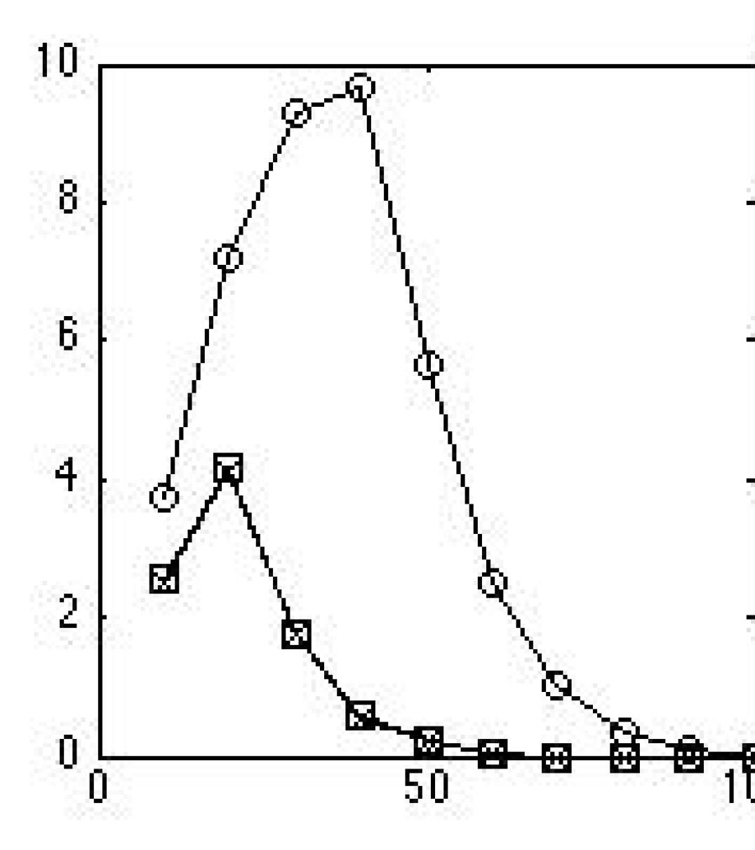
Total number of vertices, $n$

Figure 1: Number of vertices mis-clustered by TTM, HOSVD and NH-Cut as $n$ increases. The figures from left to right correspond to cases with $m=2$, 3 and 4, respectively.

We consider another example on bi-partitioning 3-uniform hypergraphs, where we fix $q=0.2$ but the gap $p$ is decreased as 0.1, 0.05 and 0.025. Figure 2 shows the errors, averaged over 50 runs, incurred by the three methods as the hypergraph grows. Note that the problem becomes harder as $p$ reduces, and the performance of HOSVD is highly affected. But, the effect is much less in case of TTM and NH-Cut. This follows from Theorem 2, where one can observe that, in the present context $\mathsf{Err}(\psi,\psi^{\prime})$ varies as $1/p^{2}$. Same holds for NH-Cut, but in the case of HOSVD, $\mathsf{Err}(\psi,\psi^{\prime})$ varies as $1/p^{4}$ making the algorithm more sensitive to reduction in probability gap.

(a) $p=0.1$                (b) $p=0.05$               (c) $p=0.025$
Error, $\mathsf{Err}(\psi,\psi^{\prime})$
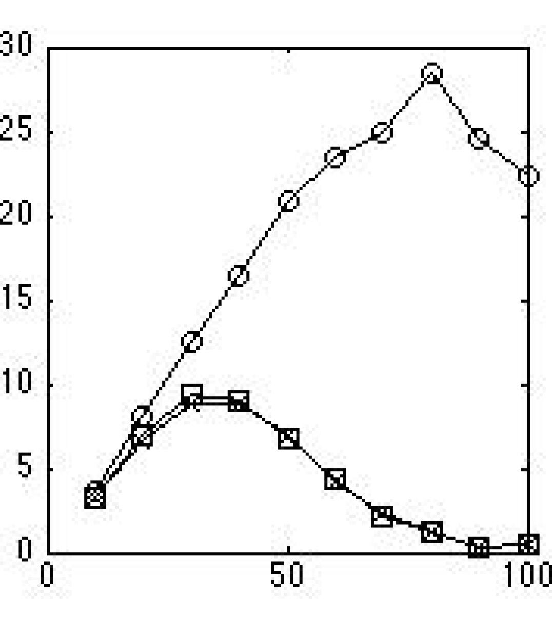
Total number of vertices, $n$

Figure 2: Number of vertices mis-clustered by TTM, HOSVD and NH-Cut as $n$ increases. The figures from left to right correspond to cases with $p=0.1$, 0.05 and 0.025, respectively.

6.2 Comparison of Hypergraph Partitioning Methods

We consider similar studies with other hypergraph partitioning methods, such as methods based on symmetric non-negative tensor factorisation (SNTF) (Shashua et al., 2006), higher order game theoretic clustering (HGT) (Rota Bulo and Pelillo, 2013) and the hMETIS algorithm widely used in VLSI community (Karypis and Kumar, 2000). For the latter two methods, we have used implementations provided by the authors.

We first compare the different algorithms under a planted model for 3-uniform hypergraphs with $k=3$ planted clusters of equal size. As before, we assume the hypergraph to be dense, $\alpha_{n}=1$, and the inter-cluster edges occur with probability $q=0.2$. We study the performance of the methods as the number of vertices $n$, and the probability gap $p$ varies. The fractional clustering error, $\frac{1}{n}\mathsf{Err}(\psi,\psi^{\prime})$, averaged over 50 runs, is reported in Figure 3.

The figure shows the previously observed trends for TTM, NH-Cut and HOSVD. In addition, it is observed that SNTF and hMETIS provide nearly similar, but marginally worse results than TTM. However, HGT uses a greedy strategy for extracting individual clusters, and hence, often identifies a majority of the vertices as outliers, thereby resulting in poor performance.

Probability gap $p$
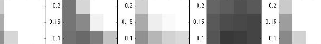
	Number of vertices in each cluster, $n/k$

Figure 3: Fractional error incurred by hypergraph partitioning algorithms under a planted model. The cluster size, $(n/k)$, and the probability gap $p$ are varied. The colour bar indicates the shade corresponding to different levels of error, with darker shade representing larger error.

Since partitioning algorithms find use in a variety of applications, we compare the performance of the above algorithms for the subspace clustering problem. In particular, we consider the line clustering problem in an ambient space of dimension 3. We randomly generate three one-dimensional subspaces, and sampled $n/k$ random points from each subspace. As mentioned in the previous section, the data points in subspace clustering problems are typically perturbed by noise. To simulate this behaviour, we add a zero mean Gaussian noise vector to each point. The covariance of the noise vectors is given as $\sigma_{a}I$, where we vary $\sigma_{a}$ to control the difficulty of the problem. We construct a weighted 3-uniform similarity hypergraph based on polar curvature of triplet of points, which is partitioned by the different methods. The fractional clustering errors are presented in Figure 4. As expected, all the methods can identify the exact subspace in the absence of noise, and the errors increase for larger $\sigma_{a}$. Apart from HGT, a good performance is observed from all the methods.

Noise level, $\sigma_{a}$
	Number of points in each subspace, $n/k$

Figure 4: Fractional error incurred by hypergraph partitioning algorithms in clustering noisy points from three intersecting lines. The cluster size, $(n/k)$, and the noise level $\sigma_{a}$ are varied. The colour bar indicates the shade corresponding to different levels of error, with darker shade representing larger error.

One can observe that the above comparisons were based on very small problems, where the hypergraph consists of at most 120 vertices. This restriction was imposed since specification of the entire affinity tensor is computationally infeasible for large hypergraphs. To demonstrate the performance of TTM in practical settings, we study its sampled variants in the subsequent sections.

6.3 Comparison of Subspace Clustering Algorithms: Synthetic Data

We now compare our method against the state of the art subspace clustering algorithms. We consider sampled variants of the TTM algorithm, i.e., TTM with uniform sampling and TTM with iterative sampling (Tetris). We note that from practical consideration, we do not consider aforementioned hypergraph partitioning methods that require computation of the entire tensor. The clustering algorithms under consideration include:

• $k$-means algorithm for clustering based on Euclidean distance,

• $k$-flats algorithm (Bradley and Mangasarian, 2000) which generalises $k$-means to subspace clustering,

• sparse subspace clustering (SSC) (Elhamifar and Vidal, 2013), which finds clusters by estimating the subspaces,

• subspace clustering using low-rank representation (LRR) (Liu et al., 2010),

• thresholding based subspace clustering (TSC) (Heckel and Bölcskei, 2013),

• faster variant of SSC using orthogonal matching pursuit (SSC-OMP) (Dyer et al., 2013),

• greedy subspace clustering using nearest subspace neighbour search and spectral clustering (NSN+Spectral) (Park et al., 2014),

• spectral curvature clustering (SCC) (Chen and Lerman, 2009), which is an iterative variant of HOSVD,

• sparse Grassmann clustering (SGC) (Jain and Govindu, 2013), yet another variation of HOSVD where some information about the eigenvectors computed in previous iterations is retained,

• Algorithm Tetris, and

• Algorithm TTM with uniform sampling, which is derived by performing a single iteration of Steps 1-14 of Algorithm Tetris.

We first focus on the problem of clustering randomly generated subspaces. In an ambient space of dimension $r_{a}=5$, we randomly generate $k=5$ subspaces each of dimension $r=3$. From each subspace, we randomly sample $n/k$ points and perturb every point with a 5-dimensional Gaussian noise vector with mean zero and covariance $\sigma_{a}I$. In Figure 5, we report the fractional error, $\frac{1}{n}\mathsf{Err}(\psi,\psi^{\prime})$, incurred by various subspace clustering algorithms when $(n/k)$ and $\sigma_{a}$ are varied. The results are averaged over 50 independent trials. We note that for existing methods, we fix the parameters as mentioned in Park et al. (2014). For Tetris and SGC, the parameters are set to the same values as SCC, where $c=100k$ and $\sigma$ as in (33) is determined by the algorithm. In case of uniformly sampled TTM, we fix $\sigma$ to be same as the value determined by Tetris. To demonstrate that sampling more edges lead to error reduction, we consider uniform sampling for two values $c=100k$ and $200k$.

Figure 5 shows that Tetris and SGC clearly outperform other methods over a wide range of settings. In particular, it can be seen that greedy methods like NSN is accurate in the absence of noise, but a drastic increase in error occurs when the data is noisy. The effect of noise is much less in hypergraph based methods like SCC, SGC or Tetris. One can also observe that the hypergraph based methods do not work well when there are very few points in each cluster (for example, 6). This is expected since, by definition, these algorithms construct 5-uniform hypergraphs $(m=r+2)$ in this case, and hence, there are very few edges $(\binom{6}{5}=6)$ with large weight for each cluster. However, with increase in number of points, there is a rapid decay in the clustering error. This also shows the consistency of these methods empirically. To this end, it seems that NSN or SSC should be recommended for small scale problems (smaller $n/k$), whereas Tetris or SGC should be the algorithm of choice for larger $n$ and possible presence of noise. Finally, we also observe that TTM with uniform sampling, even with twice the number of samples, performs quite poorly as compared to Tetris. However, with increase in the number of sampled edges, some extent of error reduction is observed.

Noise level, $\sigma_{a}$
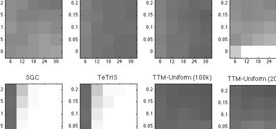
	Number of points in each subspace, $n/k$

Figure 5: Fractional error incurred by subspace clustering algorithms for synthetic data. The number of points in each subspace, $(n/k)$, and the variance of the noise vector $\sigma_{a}$ is varied. The colour bar indicates the shades for different levels of error.

6.4 Comparison of Subspace Clustering Algorithms: Motion Segmentation

The Hopkins 155 database (Tron and Vidal, 2007) contains a number of videos capturing motion of multiple objects or rigid bodies. In each video, few features are tracked along the frames, each giving rise to a motion trajectory that resides in a space of dimension twice the number of frames. One can show that under particular camera models, all trajectories corresponding to a particular rigid body motion span a subspace of dimension at most four (Tomasi and Kanade, 1992). Thus, the problem of segmenting different motions in a video can be posed as a subspace clustering problem.

The Hopkins database contains 120 sequences, each containing two motions, and 35 three motion sequences. We run above mentioned subspace clustering algorithms for purpose of motion segmentation. For existing approaches, the parameters specified in Park et al. (2014) have been used, and for Tetris and SGC, we use the parameters for SCC. TTM with uniform sampling is not considered due to its higher error rate. Table 1 reports the mean and median of the percentage errors incurred by different algorithms, where these statistics are computed over all 2-motion and 3-motion sequences. In order to remove the effect of randomisation due to sampling (for SCC, SGC, Tetris) or initialisation (for $k$-means, $k$-flats, NSN), we average the results over 20 independent trials. The average computational time (in seconds) of each algorithm for each video is also reported.

Table 1 shows that Tetris performs quite well in comparison with state of the art subspace clustering algorithms. In particular, Tetris achieves least mean error for the two motion problem. The computational time for Tetris is also much smaller than other accurate methods like SSC and LRR. The mean error achieved by Tetris is also smaller than SCC in either cases. We note here that the best known results for Hopkins 155 database is achieved by the algorithm in Jung et al. (2014), which uses techniques based on epi-polar geometry, and hence, it is not a subspace clustering algorithm. Smaller errors have also been reported in the literature when one construct larger tensors, $m=8$ (Jain and Govindu, 2013), or uses manual tuning of hyper-parameters (Ghoshdastidar and Dukkipati, 2015a). However, in either cases, computational time increases considerably.

Algorithm	2 motion (120 sequences)			3 motion (35 sequences)
	Mean (%)	Median (%)	Time (s)	Mean (%)	Median (%)	Time (s)
$k$-means	19.58	17.92	0.03	26.13	20.48	0.05
$k$-flats	13.19	10.01	0.38	15.45	14.88	0.76
SSC	1.53	0.00	0.80	4.40	0.56	1.51
LRR	2.13	0.00	0.94	4.03	1.43	1.29
SSC-OMP	16.93	13.28	0.72	27.61	23.79	1.23
TSC	18.44	16.92	0.19	28.58	29.67	0.51
NSN+Spec	3.62	0.00	0.08	8.28	2.76	0.17
SCC	2.53	0.03	0.45	6.40	1.46	0.76
SGC	3.50	0.41	0.54	9.08	5.05	0.89
Tetris	1.31	0.02	0.50	5.71	1.19	0.90

Table 1: Mean and median of clustering error and computational time for different subspace clustering algorithms on Hopkins 155 database.

7 Conclusion

In this paper, we studied the problem of partitioning uniform hypergraphs that arises in several applications in computer vision and databases. We formalised the problem by defining a normalised associativity of a partition in a uniform hypergraph that extends a similar notion used in graph literature. We showed that the task of finding a partition that maximises normalised associativity is equivalent to a tensor trace maximisation problem. We proposed a tensor spectral algorithm (TTM) to solve this problem, and following the lines of our previous works, we showed that the TTM algorithm is consistent under a planted partition model. To this end, we extended the existing model of Ghoshdastidar and Dukkipati (2014, 2017) by allowing both sparsity of edges as well as the possibility of weighted edges. Accounting for these factors makes the model more appropriate in the context of computer vision applications. We derived error bounds for the TTM approach under the planted partition model. Our bounds indicate that under mild assumptions on the sparsity of the hypergraph, TTM is weakly consistent, and the error bound for TTM is comparable that of NH-Cut, but better than the error rates for HOSVD. This fact is also validated numerically.

Weighted uniform hypergraphs have been particularly interesting in the computer vision since hypergraphs provide a natural way to represent multi-way similarities. Yet, it is computationally expensive to compute the entire affinity tensor of the hypergraph. As a consequence, several tensor sampling strategies have come into existence. We provide the first theoretical analysis of such sampling techniques in the context of uniform hypergraph partitioning. Our result suggests that consistency can be achieved even with very few sampled edges provided that one assigns a higher sampling probability for edges with larger weight. The derived sampling rate is much lower than that known in tensor literature (Bhojanapalli and Sanghavi, 2015; Jain and Oh, 2014), and our analysis also justifies the superior performance of popular sampling heuristics (Chen and Lerman, 2009; Duchenne et al., 2011). We finally proposed a iteratively sampled variant of TTM, and empirically demonstrated the potential of this method in subspace clustering and motion segmentation applications.

We conclude with the remark that this paper was motivated by practical aspects of hypergraph partitioning, and our aim was to present an approach that can be analysed theoretically, and at the same time, can compete with practical methods. While the paper manages to achieve this goal, there are several questions that still remain unanswered. We list some of the important open problems:

(i) What is the threshold for detecting planted partitions in hypergraphs?
This question was recently answered for a special model in the case of bi-partitioning (Florescu and Perkins, 2016), but more general cases have still not been explored. For instance, it would interesting to know any extension of the results in Abbe and Sandon (2016) for unweighted hypergraphs. However, this would still not provide any information in the weighted case. We noted that one of the reasons for our condition in (14) being worse by logarithmic factors was our analysis is for weighted hypergraphs. It is not known yet whether one can do better for weighted hypergraphs without making distributional assumptions on the edge weights.

(ii) What are the complicated examples? How can we deal with these cases?
Our error bound leads to a counter-intuitive conclusion that even after collapsing the tensor to a matrix, one can get better performance than direct tensor decomposition (HOSVD). The caveat here is that this result is stated for a special case, and still leaves the possibility that that there are models which do not satisfy the condition $\delta>0$, and hence, TTM does not work. In Ghoshdastidar and Dukkipati (2017), we constructed few examples, but it is not known whether HOSVD works in these cases. We also mention that the use of other tensor methods (such as power iterations) have not been analysed yet. While we showed that existing results cannot be applied due to the difference in assumptions, we do not claim that alternative tensor methods are inapplicable.

On a similar note, it is known in the case of graph partitioning that the eigen gap (quantified by $\delta$ in our results) is not the correct quantity that reflects the presence of a partition. For instance, there are planted graph models, which clearly reflect a separation of the classes, and yet $\delta$ is not positive. It would be interesting to see how one can deal with such examples in the case of hypergraphs. An alternative approach in such cases is to quantify the separation by the minimum difference (or distance) between the $k$ rows of $\mathbf{B}$, which is a matrix for graphs. For uniform hypergraphs, a similar quantity would be the difference between the $(m-1)$-order slices of the tensor $\mathbf{B}$, but it is not clear yet how such a condition can be incorporated into the analysis of hypergraph partitioning.

(iii) What is the minimum sample size for achieving weak consistency?
Similar in spirit to the first problem, one can ask what is the minimum sampling rate required to achieve weak consistency irrespective of the partitioning algorithm. We have not made any attempt to answer this question, and surprisingly, the question is open even in graph partitioning. While column sampling techniques (Drineas et al., 2006) are often used in conjunction with spectral clustering, the error rate for this combination is not known.

(iv) How well does TTM extend for other higher order learning problems?
While TTM unifies a wide variety of higher order learning methods, the special cases studies in this paper were restricted to clustering problems. However, other problems like tensor matching can also be modelled as partitioning uniform hypergraph with two partitions of widely different sizes (Duchenne et al., 2011). In principle, this problem has a flavour quite similar to that of the well known planted clique problem (Alon et al., 1998). The state of the art algorithms in tensor matching rely on tensor power iterations, and in Ghoshdastidar and Dukkipati (2017), we showed that a naive use of NH-Cut does not fare well. We feel that in this particular setting, better theoretical guarantees can be achieved by power iteration based approaches.

Acknowledgments

We thank the reviewers for useful suggestions and key references. During this work, D. Ghoshdastidar was supported by the 2013 Google Ph.D. Fellowship in Statistical Learning Theory. This work is also partly supported by the Science and Engineering Research Board through the grant SERB:SB/S3/EECE/093/2014.

A Proofs of Technical Lemmas and Corollaries

Here, we sequentially present the proofs of lemmas and corollaries stated in the paper. We begin with the calculations that lead to (10).

A.1 Proof of Equation (10)

We recall that the entries of $Y^{(l)}$ is simply $Y_{ij}^{(l)}=\frac{\mathds{1}\{i\in\mathcal{V}_{j}\}}{(\textup{vol}(\mathcal{V}_{j}))^{\beta_{l}}}$. The claimed relation follows by computing diagonal entries of $\mathbf{A}\times_{1}{Y^{(1)}}^{T}\times_{2}{Y^{(2)}}^{T}\times_{3}\ldots\times_{m}{Y^{(m)}}^{T}$, which are given by

$$\left(\mathbf{A}\times_{1}{Y^{(1)}}^{T}\times_{2}\ldots\times_{m}{Y^{(m)}}^{T}\right)_{j\ldots j} =\sum_{i_{1},\ldots,i_{m}=1}^{n}\mathbf{A}_{i_{1}\ldots i_{m}}Y_{i_{1}j}^{(1)}\ldots Y_{i_{m}j}^{(m)}$$

$$=m!\sum_{i_{1}<\ldots<i_{m}}\mathbf{A}_{i_{1}\ldots i_{m}}\frac{\mathds{1}\{i_{1},\ldots,i_{m}\in\mathcal{V}_{j}\}}{(\textup{vol}(\mathcal{V}_{j}))^{\beta_{1}+\ldots+\beta_{m}}}\;,$$

where we use the symmetry of the terms to group all $m!$ permutations of every distinct $i_{1},\ldots,i_{m}$. Since $\sum_{l}\beta_{l}=1$, the denominator is simply $\textup{vol}(\mathcal{V}_{j})$, whereas the indicator in the numerator counts only the edges $e\subset\mathcal{V}_{j}$ and $\mathbf{A}_{i_{1}\ldots i_{m}}$ provides the weights. So the above quantity is simply $m!\frac{\textup{assoc}(\mathcal{V}_{j})}{\textup{vol}(\mathcal{V}_{j})}$, and summing over all diagonal entries results in the normalised associativity, scaled by $m!$.

A.2 Proof of Corollary 3

We begin by computing $\mathcal{A}$ as defined in (12)

$$\mathcal{A}_{ij}=\left\{\begin{array}[]{ll}(m-2)!\alpha_{n}\left(p\binom{\frac{n}{k}-2}{m-2}+q\binom{n-2}{m-2}\right)&\text{if }i\neq j,\psi_{i}=\psi_{j}\\ \\ (m-2)!\alpha_{n}q\binom{n-2}{m-2}&\text{if }i\neq j,\psi_{i}\neq\psi_{j}\\ \\ 0&\text{if }i=j.\end{array}\right.$$

From the definition of $G$, $\mathcal{D}_{\min}$ and $\delta$, one can compute that

$$\mathcal{D}_{\min}=(m-1)!\alpha_{n}\left(p\binom{\frac{n}{k}-1}{m-1}+q\binom{n-1}{m-1}\right)\;,$$ (34)

and

$$\delta=\lambda_{k}(G)\frac{n}{k\mathcal{D}_{\min}}=\frac{(m-2)!\alpha_{n}pn}{k\mathcal{D}_{\min}}\binom{\frac{n}{k}-2}{m-2}$$ (35)

We need to validate that the conditions in (14), or equivalently (18), are satisfied. Given $\alpha_{n}=1$, one can see that $\mathcal{D}_{\min}=\Theta(n^{m-1})$ easily satisfies first condition of (18) for large $n$. Also

$$\delta^{2}\mathcal{D}_{\min}=\Theta\left(\left(\frac{n}{k}\right)^{2m-2}\frac{1}{\mathcal{D}_{\min}}\right)=\Theta\left(\frac{n^{m-1}}{k^{2m-2}}\right)=\Omega\left(n^{(m-1)/2}(\ln n)^{2m-2}\right)\;,$$

taking into account that $k=O\left(\frac{n^{1/4}}{\ln n}\right)$. Thus, the second condition in (18) also holds for large $n$ and for all $m\geq 2$. Subsequently, one can applying the bound in (15) to claim that $\mathsf{Err}(\psi,\psi^{\prime})=O\left(\frac{n^{(3-m)/2}}{(\ln n)^{2m-3}}\right)$ with probability $(1-o(1))$.

A.3 Proof of Corollary 4

For $k=O(\ln n)$, one can verify that (14) holds if $\mathcal{D}_{\min}=\Omega\left(\frac{(\ln n)^{3}}{\delta^{2}}\right)$. From (34) and (35), we have $\mathcal{D}_{\min}=\Theta(\alpha_{n}n^{m-1})$ and $\delta^{2}\mathcal{D}_{\min}=\Omega\left(\alpha_{n}n^{m-1}(\ln n)^{2-2m}\right)$. Hence, choosing $\alpha_{n}\geq\frac{C(\ln n)^{2m+1}}{n^{m-1}}$ for sufficiently large $C$ ensures that (18) is satisfied. Subsequently with probability $\left(1-O\left(n^{-2}+(\ln n)^{-1/4}\right)\right)=(1-o(1))$, we obtain an error bound

$$\mathsf{Err}(\psi,\psi^{\prime})=O\left(\frac{n\ln n}{\delta^{2}\mathcal{D}_{\min}}\right)=O\left(\frac{n\ln n}{\alpha_{n}n^{m-1}(\ln n)^{2-2m}}\right)=O\left(\frac{n}{(\ln n)^{2}}\right)=o(n)\;,$$

which completes the proof.

A.4 Proof of Lemma 1

The proof is along the lines of the proof of Lemma 4.5 in Ghoshdastidar and Dukkipati (2017). We still include a sketch of the proof since the quantities involved are different from the terms dealt in the mentioned paper. From the discussions following (12), one can see that the matrix $\mathcal{A}$ may be expressed as

$$\mathcal{A}=ZGZ^{T}-J\;,$$

where $J\in\mathbb{R}^{n\times n}$ is diagonal with $J_{ii}=G_{\psi_{i}\psi_{i}}$. Following the arguments of Ghoshdastidar and Dukkipati (2017), one can show that there is a matrix $\mathcal{G}\in\mathbb{R}^{k\times k}$ with eigen decomposition $\mathcal{G}=U\Lambda_{1}U^{T}$ such that $\mathcal{L}\mathcal{X}=\mathcal{X}\Lambda_{1}$, where $\mathcal{X}=Z(Z^{T}Z)^{-1/2}U$, and it satisfies $\mathcal{X}^{T}\mathcal{X}=I$. Thus, the columns of $\mathcal{X}$ are orthonormal eigenvectors of $\mathcal{L}$ corresponding to the eigenvalues in $\Lambda_{1}$. It is also known that the other $(n-k)$ orthonormal eigenvectors correspond to eigenvalues from the set $\left\{-\frac{J_{ii}}{\mathcal{D}_{ii}}:{1\leq i\leq n}\right\}$.

Thus, to prove the claim we need to ensure that $\mathcal{X}$ corresponds to the dominant eigenvectors of $\mathcal{L}$, or in other words,

$$\lambda_{k}(\mathcal{G})>\max_{1\leq i\leq n}\left(-\frac{J_{ii}}{\mathcal{D}_{ii}}\right)=-\min_{1\leq i\leq n}\frac{G_{\psi_{i}\psi_{i}}}{\mathcal{D}_{ii}}\;.$$ (36)

A lower bound on $\lambda_{k}(\mathcal{G})$ can be derived from Rayleigh’s principle and Weyl’s inequality as

$$\lambda_{k}(\mathcal{G})\geq\lambda_{k}(G)\min_{1\leq i\leq n}\frac{(Z^{T}Z)_{\psi_{i}\psi_{i}}}{\mathcal{D}_{ii}}-\max_{1\leq i\leq n}\frac{G_{\psi_{i}\psi_{i}}}{\mathcal{D}_{ii}}\;.$$

Noting that $(Z^{T}Z)_{jj}=n_{j}$, size of cluster-$j$, one can readily see from above that if $\delta>0$, then (36) is satisfied and hence, $\mathcal{X}$ contains the dominant eigenvectors. It is also useful to note that $\delta\leq\lambda_{k}(\mathcal{L})-\lambda_{k+1}(\mathcal{L})$, i.e., $\delta$ is a lower bound on the eigen gap between the $k^{th}$ and $(k+1)^{th}$ largest eigenvalues of $\mathcal{L}$. This fact is used later in the proof of Lemma 7.

A.5 Proof of Lemma 6

We begin the proof with the claims that if $\mathcal{D}_{\min}>9(m-1)!\ln n$, then

$$\mathsf{P}_{H}\left(\max_{1\leq i\leq n}\left|\frac{D_{ii}}{\mathcal{D}_{ii}}-1\right|>3\sqrt{\frac{(m-1)!\ln n}{\mathcal{D}_{\min}}}\right)\leq\frac{2}{n^{2}}\;,$$ (37)

and

$$\mathsf{P}_{H}\left(\|\mathcal{D}^{-1/2}(A-\mathcal{A})\mathcal{D}^{-1/2}\|_{2}>3\sqrt{\frac{(m-1)!\ln n}{\mathcal{D}_{\min}}}\right)\leq\frac{2}{n^{2}}\;.$$ (38)

We now bound $\|L-\mathcal{L}\|_{2}$ as

$$\|L-\mathcal{L}\|_{2} \leq\|\mathcal{D}^{-1/2}A\mathcal{D}^{-1/2}-D^{-1/2}AD^{-1/2}\|_{2}+\|\mathcal{D}^{-1/2}A\mathcal{D}^{-1/2}-\mathcal{D}^{-1/2}\mathcal{A}\mathcal{D}^{-1/2}\|_{2}\;.$$

We expand the first term as

$$\|\mathcal{D}^{-1/2}A\mathcal{D}^{-1/2}- D^{-1/2}AD^{-1/2}\|_{2}$$

$$\leq\|(\mathcal{D}^{-1/2}-D^{-1/2})A\mathcal{D}^{-1/2}+D^{-1/2}A(\mathcal{D}^{-1/2}-D^{-1/2})\|_{2}$$

$$\leq\|(\mathcal{D}^{-1}D)^{1/2}-I\|_{2}\|(D\mathcal{D}^{-1})^{1/2}\|_{2}+\|(\mathcal{D}^{-1}D)^{1/2}-I\|_{2},$$

where the last inequality follows since $\|D^{-1/2}AD^{-1/2}\|_{2}=1$. Also, note that

$$\|(\mathcal{D}^{-1}D)^{1/2}-I\|_{2}=\max_{1\leq i\leq n}\left|\sqrt{\frac{D_{ii}}{\mathcal{D}_{ii}}}-1\right|\leq\max_{1\leq i\leq n}\left|{\frac{D_{ii}}{\mathcal{D}_{ii}}}-1\right|.$$

Combining above arguments, we can write

$$\|L-\mathcal{L}\|_{2}\leq\max_{1\leq i\leq n}\left|{\frac{D_{ii}}{\mathcal{D}_{ii}}}-1\right|\left(2+\max_{1\leq i\leq n}\left|{\frac{D_{ii}}{\mathcal{D}_{ii}}}-1\right|\right)+\|\mathcal{D}^{-1/2}A\mathcal{D}^{-1/2}-\mathcal{D}^{-1/2}\mathcal{A}\mathcal{D}^{-1/2}\|_{2}.$$ (39)

Using the bounds in (37) and (38) along with the fact that $3\sqrt{\frac{(m-1)!\ln n}{\mathcal{D}_{\min}}}<1$, one arrives at the claim.

We now prove the concentration bound in (37). Observe that

$$D_{ii}=\sum_{j=1}^{n}A_{ij}=\sum_{i_{2},\ldots,i_{m}=1}^{n}\mathbf{A}_{ii_{2}\ldots i_{m}}=(m-1)!\sum_{e\in\mathcal{E}:e\ni i}w_{e}\;,$$

where the last equality holds since the summation over all $i_{2},\ldots,i_{m}$ counts each edge containing node-$i$ $(m-1)!$ times. Since, $D_{ii}$ is a sum of independent random variables, we can use Bernstein inequality to obtain for any $t>0$,

$$\mathsf{P}_{H}\left(|D_{ii}-\mathcal{D}_{ii}|>t\mathcal{D}_{ii}\right) =\mathsf{P}_{H}\left(\left|\sum_{e\in\mathcal{E}:e\ni i}w_{e}-\mathsf{E}_{H}[w_{e}]\right|>\frac{t\mathcal{D}_{ii}}{(m-1)!}\right)$$

$$\leq 2\exp\left(\frac{-\left(\frac{t\mathcal{D}_{ii}}{(m-1)!}\right)^{2}}{2\sum\limits_{e\in\mathcal{E}:e\ni i}\mathsf{Var}_{H}(w_{e})+\frac{2}{3}\frac{t\mathcal{D}_{ii}}{(m-1)!}}\right)\;.$$ (40)

Since $w_{e}\in[0,1]$, we have

$$\sum\limits_{e\in\mathcal{E}:e\ni i}\mathsf{Var}_{H}(w_{e})\leq\sum\limits_{e\in\mathcal{E}:e\ni i}\mathsf{E}_{H}[w_{e}]=\frac{\mathcal{D}_{ii}}{(m-1)!}\;.$$

Substituting this in (40), we have

$$\mathsf{P}_{H}\left(|D_{ii}-\mathcal{D}_{ii}|>t\mathcal{D}_{ii}\right)\leq 2\exp\left(-\frac{t^{2}\mathcal{D}_{ii}}{3(m-1)!}\right)\leq 2\exp\left(-\frac{t^{2}\mathcal{D}_{\min}}{3(m-1)!}\right).$$

The bound in (37) follows from above by setting $t=3\sqrt{\frac{(m-1)!\ln n}{\mathcal{D}_{\min}}}$, and using a union bound over all $i=1,\ldots,n$.

Finally, we derive (38) using matrix Bernstein inequality (Tropp, 2012, Theorem 1.4), which states that for independent, symmetric, random matrices $Y_{1},\ldots,Y_{M}\in\mathbb{R}^{n\times n}$ with $\mathsf{E}_{H}[Y_{i}]=0$ and $\|Y_{i}\|_{2}\leq R$ almost surely, one has

$$\mathsf{P}\left(\left\|\sum_{i=1}^{M}Y_{i}\right\|_{2}>t\right)\leq n\exp\left(\frac{-{t^{2}}}{2\|\sum_{i}\mathsf{E}[Y_{i}^{2}]\|_{2}+\frac{2Rt}{3}}\right)$$ (41)

for any $t>0$. Owing to the representation in (19), one can write

$$\mathcal{D}^{-1/2}(A-\mathcal{A})\mathcal{D}^{-1/2}=\sum_{e\in\mathcal{E}}(m-2)!\left(w_{e}-\mathsf{E}_{H}[w_{e}]\right)\mathcal{D}^{-1/2}R_{e}\mathcal{D}^{-1/2}$$

as a sum of independent, zero mean random matrices. One can verify that $\|R_{e}\|_{2}\leq(m-1)$, and hence,

$$\left\|(m-2)!\left(w_{e}-\mathsf{E}_{H}[w_{e}]\right)\mathcal{D}^{-1/2}R_{e}\mathcal{D}^{-1/2}\right\|_{2}\leq\frac{(m-1)!}{\mathcal{D}_{\min}}\;.$$

In addition, one can bound

$$\left\|\sum_{e\in\mathcal{E}}\mathsf{E}_{H}\left[\left((m-2)!\left(w_{e}-\mathsf{E}_{H}[w_{e}]\right)\mathcal{D}^{-1/2}R_{e}\mathcal{D}^{-1/2}\right)^{2}\right]\right\|_{2}$$

$$=((m-2)!)^{2}\left\|\sum_{e\in\mathcal{E}}\mathsf{Var}_{H}(w_{e})\mathcal{D}^{-1/2}R_{e}\mathcal{D}^{-1}R_{e}\mathcal{D}^{-1/2}\right\|_{2}$$

$$=((m-2)!)^{2}\left\|\sum_{e\in\mathcal{E}}\mathsf{Var}_{H}(w_{e})\left(\mathcal{D}^{-1}R_{e}\right)^{2}\right\|_{2}$$

$$\leq((m-2)!)^{2}\max_{1\leq i\leq n}\sum_{j=1}^{n}\sum_{e\in\mathcal{E}}\mathsf{Var}_{H}(w_{e})\left(\left(\mathcal{D}^{-1}R_{e}\right)^{2}\right)_{ij}$$

$$\leq\frac{((m-2)!)^{2}}{\mathcal{D}_{\min}}\max_{1\leq i\leq n}\frac{1}{\mathcal{D}_{ii}}\sum_{e\in\mathcal{E}}\mathsf{E}_{H}(w_{e})\sum_{j=1}^{n}\left(R_{e}^{2}\right)_{ij}\;.$$

Here, the first inequality holds due to Gerschgorin’s theorem. Observing that the row sum of $R_{e}^{2}$ is at most $(m-1)^{2}$, the expression can be simplified to show that the quantity is bounded from above by $\frac{(m-1)!}{\mathcal{D}_{\min}}$. Setting $t=3\sqrt{\frac{(m-1)!\ln n}{\mathcal{D}_{\min}}}$ in (41), and combining above arguments, one arrives at (38). This completes the proof.

A.6 Proof of Corollary 10

We begin by characterising $\beta$ for either sampling methods. Note that $\beta\geq\max_{e}\frac{w_{e}}{p_{e}}$. Since, $|\mathcal{E}|=\binom{n}{m}$, it follows that for uniform sampling $p_{e}=\binom{n}{m}^{-1}$ for all $e$, and hence, an appropriate choice of $\beta=\binom{n}{m}$. On the other hand, for the sampling in (27), $\max_{e}\frac{w_{e}}{p_{e}}=\sum_{e}w_{e}$. Using Bernstein inequality, one may easily bound this term from above by $2\sum_{e}\mathsf{E}_{H}[w_{e}]\leq 2\alpha_{n}\binom{n}{m}$, where the bound holds with probability $(1-n^{-2})$.

Thus, ignoring constants factors, one may set $\beta=\xi n^{m}$, where $\xi=1$ for uniform sampling and $\alpha_{n}$ for weighted sampling. The conditions in (28) follow directly from (25) and $d,\delta$ computed in the proof of Corollary 3.

A.7 Proof of Lemma 11

Let $\beta$ be defined as in Theorem 9 and $D_{\min}=\min\limits_{1\leq i\leq n}D_{ii}$. Assume that

$$\mathcal{D}_{\min}>36(m-1)!\ln n\quad\text{ and }\quad N>9\left(1+\frac{2\beta(m-1)!}{\mathcal{D}_{\min}}\right)\ln n\;.$$ (42)

Also let $\Gamma$ denote the event

$$\Gamma=\left\{{D_{\min}}>\frac{\mathcal{D}_{\min}}{2}\right\}\bigcap\left\{\max_{e\in\mathcal{E}}\frac{w_{e}}{p_{e}}\leq\beta\right\}.$$

Then, conditioned on a given random hypergraph and the event $\Gamma$, we claim that the following bounds hold with probability $(1-\frac{2}{n^{2}})$,

$$\max_{1\leq i\leq n}\left|\frac{\widehat{D}_{ii}}{D_{ii}}-1\right|\leq 3\sqrt{\frac{\ln n}{N}\left(1+\frac{2\beta(m-1)!}{\mathcal{D}_{\min}}\right)}\;.$$ (43)

and

$$\|D^{-1/2}(\widehat{A}-A)D^{-1/2}\|_{2}\leq 3\sqrt{\frac{\ln n}{N}\left(1+\frac{2\beta(m-1)!}{\mathcal{D}_{\min}}\right)}\;.$$ (44)

Assuming that the above hold, we now derive a bound on $\|\widehat{L}-L\|_{2}$ in the following way. First, note that the bounds in (43) and (44) are with respect to a conditional probability measure, and need to be converted into a bound with respect to the joint probability measure $\mathsf{P}_{S,H}$. This is not hard to derive as one can see in the case of (44), where one can write

$$\mathsf{P}_{S,H}\left(\|D^{-1/2}(\widehat{A}-A)D^{-1/2}\|_{2}>3\sqrt{\frac{\ln n}{N}\left(1+\frac{2\beta(m-1)!}{\mathcal{D}_{\min}}\right)}\right)$$

$$=\mathsf{E}_{H}\left[\mathsf{P}_{S|H}\left(\|D^{-1/2}(\widehat{A}-A)D^{-1/2}\|_{2}>3\sqrt{\frac{\ln n}{N}\left(1+\frac{2\beta(m-1)!}{\mathcal{D}_{\min}}\right)}\right)\right]$$

$$\leq\mathsf{P}_{H}\left(\Gamma\right)\mathsf{E}_{H|\Gamma}\left[\mathsf{P}_{S|H,\Gamma}\left(\|D^{-1/2}(\widehat{A}-A)D^{-1/2}\|_{2}>3\sqrt{\frac{\ln n}{N}\left(1\text{+}\frac{2\beta(m-1)!}{\mathcal{D}_{\min}}\right)}\right)\right]+\mathsf{P}_{H}\left(\Gamma^{c}\right)$$

$$=O\left(\frac{1}{n^{2}}\right)+\mathsf{P}_{H}\left(\Gamma^{c}\right),$$ (45)

where the inequalities follow by observing that all the quantities are smaller than one, and the first term is bounded due to (44). For bounding $\mathsf{P}_{H}\left(\Gamma^{c}\right)$, note that from (37), it follows that with probability $(1-O(n^{-2}))$, for all $i=1,\ldots,n$,

$$D_{ii}>\mathcal{D}_{ii}\left(1-3\sqrt{\frac{(m-1)!\ln n}{\mathcal{D}_{\min}}}\right).$$

Hence, if $\mathcal{D}_{\min}>36(m-1)!\ln n$, then

$$D_{\min}>\mathcal{D}_{\min}\left(1-3\sqrt{\frac{(m-1)!\ln n}{\mathcal{D}_{\min}}}\right)>\frac{\mathcal{D}_{\min}}{2}\;.$$

This fact, along with the assumption on $\beta$, shows that $\mathsf{P}_{H}(\Gamma^{c})=o(1)$, and so, the upper bound on $\|D^{-1/2}(\widehat{A}-A)D^{-1/2}\|_{2}$ holds with probability $(1-o(1))$ even with respect to joint probability measure. Similar result also holds for (43). Subsequently, we follow the arguments leading to (39) to conclude that

$$\|\widehat{L}-L\|_{2} \leq\max_{1\leq i\leq n}\left|{\frac{\widehat{D}_{ii}}{D_{ii}}}-1\right|\left(2+\max_{1\leq i\leq n}\left|{\frac{\widehat{D}_{ii}}{D_{ii}}}-1\right|\right)+\|D^{-1/2}(\widehat{A}-A)D^{-1/2}\|_{2}$$

$$\leq 12\sqrt{\frac{\ln n}{N}\left(1+\frac{2\beta(m-1)!}{\mathcal{D}_{\min}}\right)}\;,$$

where the last inequality holds with probability $(1-O(n^{-2}))$ under the conditions stated in (42). To complete the proof, we derive the bounds (43) and (44), which again rely on the use of Bernstein inequality. For this, observe that

$$\widehat{D}_{ii}=\frac{(m-2)!}{N}\sum_{j=1}^{n}\sum_{e\in\mathcal{I}}\frac{w_{e}}{p_{e}}(R_{e})_{ij}=\frac{(m-1)!}{N}\sum_{e\in\mathcal{I}}\frac{w_{e}}{p_{e}}\mathds{1}\{i\in e\}\;,$$

where for each $e\in\mathcal{I}$,

$$\mathsf{E}_{S|H,\Gamma}\left[\frac{w_{e}}{p_{e}}\mathds{1}\{i\in e\}\right] =\sum_{e^{\prime}\in\mathcal{E}:e^{\prime}\ni i}p_{e^{\prime}}\frac{w_{e^{\prime}}}{p_{e^{\prime}}}=\frac{D_{ii}}{(m-1)!}\;,$$

$$\mathsf{Var}_{S|H,\Gamma}\left[\frac{w_{e}}{p_{e}}\mathds{1}\{i\in e\}\right] =\sum_{e^{\prime}\in\mathcal{E}:e^{\prime}\ni i}\frac{w_{e^{\prime}}^{2}}{p_{e^{\prime}}}-\left(\frac{D_{ii}}{(m-1)!}\right)^{2}\leq\left(\beta-\frac{D_{ii}}{(m-1)!}\right)\frac{D_{ii}}{(m-1)!}\;,$$

and almost surely with respect to $\mathsf{P}_{S|H,\Gamma}$,

$$\left|\frac{w_{e}}{p_{e}}\mathds{1}\{i\in e\}-\frac{D_{ii}}{(m-1)!}\right| \leq\left(\beta+\frac{D_{ii}}{(m-1)!}\right)\;.$$

Define $t=3\sqrt{\frac{\ln n}{N}\left(1+\frac{2\beta(m-1)!}{\mathcal{D}_{\min}}\right)}$. Since the samples $e\in\mathcal{I}$ are independent and identically distributed, we can use Bernstein inequality to write

$$\mathsf{P}_{S|H,\Gamma} \left(|\widehat{D}_{ii}-D_{ii}|>tD_{ii}\right)$$

$$=\mathsf{P}_{S|H,\Gamma}\left(\left|\sum_{e\in\mathcal{I}}\frac{w_{e}}{p_{e}}\mathds{1}\{i\in e\}-\frac{D_{ii}}{(m-1)!}\right|>\frac{NtD_{ii}}{(m-1)!}\right)$$

$$\leq 2\exp\left(\frac{-\frac{N^{2}t^{2}D_{ii}^{2}}{(m-1)!}}{2N\left(\beta-\frac{D_{ii}}{(m-1)!}\right)\frac{D_{ii}}{(m-1)!}+\frac{2}{3}\frac{NtD_{ii}}{(m-1)!}\left(\beta+\frac{D_{ii}}{(m-1)!}\right)}\right)$$

$$\leq 2\exp\left(\frac{-\frac{ND_{ii}t^{2}}{(m-1)!}}{\frac{2}{3}\left(4\beta-2\frac{D_{ii}}{(m-1)!}\right)}\right)$$

$$\leq 2\exp\left(\frac{-\frac{N\mathcal{D}_{\min}t^{2}}{2(m-1)!}}{\frac{2}{3}\left(4\beta+2\frac{\mathcal{D}_{\min}}{(m-1)!}\right)}\right)\leq\frac{2}{n^{3}}\;.$$

The inequalities are derived using above relations, and the definition of $\Gamma$. From above, (43) follows from union bound.

To prove (44), observe from (24) that

$$D^{-1/2}\widehat{A}D^{-1/2}=\frac{1}{N}\sum_{e\in\mathcal{I}}(m-2)!\frac{w_{e}}{p_{e}}D^{-1/2}R_{e}D^{-1/2}$$

is a sum of independent random matrices with

$$\mathsf{E}_{S|H,\Gamma}\left[(m-2)!\frac{w_{e}}{p_{e}}D^{-1/2}R_{e}D^{-1/2}\right]=D^{-1/2}AD^{-1/2}$$

and

$$\left\|(m-2)!\frac{w_{e}}{p_{e}}D^{-1/2}R_{e}D^{-1/2}-D^{-1/2}AD^{-1/2}\right\|_{2} \leq(m-2)!\beta\|D^{-1/2}R_{e}D^{-1/2}\|_{2}+1$$

$$\leq\left(\frac{2\beta(m-1)!}{\mathcal{D}_{\min}}+1\right)\;.$$

The first bound uses the fact $\|D^{-1/2}AD^{-1/2}\|_{2}=1$ and the second follows since $D_{\min}>\frac{1}{2}\mathcal{D}_{\min}$ and $\|R_{e}\|_{2}\leq(m-1)$. We can also bound the norm of the variance term as

$$\left\|\mathsf{E}_{S|H,\Gamma}\left[\left((m-2)!\frac{w_{e}}{p_{e}}D^{-1/2}R_{e}D^{-1/2}-D^{-1/2}AD^{-1/2}\right)^{2}\right]\right\|_{2}$$

$$=\left\|-\left(D^{-1/2}AD^{-1/2}\right)^{2}+((m-2)!)^{2}\sum_{e\in\mathcal{E}}\frac{w_{e}^{2}}{p_{e}}D^{-1/2}R_{e}D^{-1}R_{e}D^{-1/2}\right\|_{2}$$

$$\leq 1+\frac{((m-2)!)^{2}\beta}{D_{\min}}\left\|\sum_{e\in\mathcal{E}}w_{e}D^{-1}(R_{e})^{2}\right\|_{2}\leq\left(1+\frac{2\beta(m-1)!}{\mathcal{D}_{\min}}\right)\;.$$

Using these relations and the matrix Bernstein inequality, the bound in (44) can be derived quite similar to the derivation of (38).

References

- Abbe and Sandon (2016) E. Abbe and C. Sandon. Achieving the KS threshold in the general stochastic block model with linearized acyclic belief propagation. In Advances in Neural Information Processing Systems (NIPS), 2016.
- Agarwal et al. (2005) S. Agarwal, J. Lim, L. Zelnik-Manor, P. Perona, D. Kriegman, and S. Belongie. Beyond pairwise clustering. In IEEE Conference on Computer Vision and Pattern Recognition (CVPR), pages 838–845, 2005.
- Agarwal et al. (2006) S. Agarwal, K. Branson, and S. Belongie. Higher order learning with graphs. In International Conference on Machine Learning (ICML), pages 17–24, 2006.
- Alon et al. (1998) N. Alon, M. Krivelvich, and B. Sudakov. Finding a large hidden clique in a random graph. In ACM-SIAM Symposium on Discrete Algorithms (SODA), pages 594–598, 1998.
- Anandkumar et al. (2014) A. Anandkumar, R. Ge, D. Hsu, and S. M. Kakade. A tensor approach to learning mixed membership community models. Journal of Machine Learning Research, 15:2239–2312, 2014.
- Anandkumar et al. (2015) A. Anandkumar, R. Ge, and M. Janzamin. Learning overcomplete latent variable models through tensor methods. In Conference on Learning Theory (COLT), 2015.
- Arias-Castro et al. (2011) E. Arias-Castro, G. Chen, and G. Lerman. Spectral clustering based on local linear approximations. Electronic Journal of Statistics, 5:1537–1587, 2011.
- Bapst and Coja-Oghlan (2015) V. Bapst and A. Coja-Oghlan. The condensation phase transition in the regular k-SAT model. arXiv preprint, arXiv:1507.03512, 2015.
- Belkin et al. (2004) M. Belkin, I. Matveeva, and P. Niyogi. Regularization and semi-supervised learning on large graphs. In Conference on Learning Theory (COLT), 2004.
- Berge (1984) C. Berge. Hypergraphs: Combinatorics of Finite Sets, volume 45. Elsevier, 1984.
- Bernstein (1908) F. Bernstein. Zur theorie der trigonometrischen Reihen. Leipz. Bet., 60:325–338, 1908.
- Bhaskara et al. (2014) A. Bhaskara, M. Charikar, A. Moitra, and A. Vijayaraghavan. Smoothed analysis of tensor decompositions. In ACM Symposium on Theory of Computing (STOC), pages 594–603, 2014.
- Bhojanapalli and Sanghavi (2015) S. Bhojanapalli and S. Sanghavi. A new sampling technique for tensors. arXiv preprint, arXiv:1502.05023, 2015.
- Bolla (1993) M. Bolla. Spectra, Euclidean representations and clusterings of hypergraphs. Discrete Mathematics, 117(1):19–39, 1993.
- Boutsidis et al. (2015) C. Boutsidis, A. Gittens, and P. Kambadur. Spectral clustering via the power method - provably. In International Conference on Machine Learning (ICML), 2015.
- Bradley and Mangasarian (2000) P. S. Bradley and O. L. Mangasarian. -plane clustering. Journal of Global Optimization, 16:23–32, 2000.
- Chen and Lerman (2009) G. Chen and G. Lerman. Spectral curvature clustering. International Journal of Computer Vision, 81(3):317–330, 2009.
- Comon (2001) P. Comon. From source separation to blind equalization: Contrast based approaches. In International Conference on Image and Signal Processing, 2001.
- Comon et al. (2008) P. Comon, G. Golub, L. H. Lim, and B. Mourrain. Symmetric tensors and symmetric tensor rank. SIAM Journal of Matrix Analysis and Applications, 30(3):1254–1279, 2008.
- Cour et al. (2007) T. Cour, P. Srinivasan, and J. Shi. Balanced graph matching. In Advances in Neural Information Processing Systems (NIPS), 2007.
- De Lathauwer et al. (2000) L. De Lathauwer, B. De Moor, and J. Vandewalle. A multilinear singular value decomposition. SIAM Journal on Matrix Analysis and Applications, 21(4):1253–1278, 2000.
- Drineas et al. (2006) P. Drineas, R. Kannan, and M. W. Mahoney. Fast Monte Carlo algorithms for matrices I: Approximating matrix multiplication. SIAM Journal on Computing, 36(1):132–157, 2006.
- Duchenne et al. (2011) O. Duchenne, F. Bach, I.-S. Kweon, and J. Ponce. A tensor-based algorithm for high-order graph matching. IEEE Transactions on Pattern Analysis and Machine Intelligence, 33(12):2383–2395, 2011.
- Dyer et al. (2013) E. L. Dyer, A. C. Sankaranarayanan, and R. G. Baraniuk. Greedy feature selection for subspace clustering. Journal of Machine Learning Research, 14(1):2487–2517, 2013.
- Elhamifar and Vidal (2013) E. Elhamifar and R. Vidal. Sparse subspace clustering: Algorithm, theory, and applications. IEEE Transactions on Pattern Analysis and Machine Intelligence, 35(11):2765–2781, 2013.