.pspdf.pdfps2pdf -dEPSCrop -dNOSAFER #1

ROBUST ESTIMATION OF PROPENSITY SCORE WEIGHTS

VIA SUBCLASSIFICATION

¹Linbo Wang, ²Yuexia Zhang, ³Thomas S. Richardson, ⁴Xiao-Hua Zhou

^1,2University of Toronto, ³University of Washington, ⁴Peking University

Abstract: Weighting estimators based on propensity scores are widely used for causal estimation in a variety of contexts, such as observational studies, marginal structural models and interference. They enjoy appealing theoretical properties such as consistency and possible efficiency under correct model specification. However, this theoretical appeal may be diminished in practice by sensitivity to misspecification of the propensity score model. To improve on this, we borrow an idea from an alternative approach to causal effect estimation in observational studies, namely subclassification estimators. It is well known that compared to weighting estimators, subclassification methods are usually more robust to model misspecification. In this paper, we first discuss an intrinsic connection between the seemingly unrelated weighting and subclassification estimators, and then use this connection to construct robust propensity score weights via subclassification. We illustrate this idea by proposing so-called full-classification weights and accompanying estimators for causal effect estimation in observational studies. Our novel estimators are both consistent and robust to model misspecification, thereby combining the strengths of traditional weighting and subclassification estimators for causal effect estimation from observational studies. Numerical studies show that the proposed estimators perform favorably compared to existing methods.

Key words and phrases: Causal inference; Inverse probability weighting; Observational studies

1 Introduction

The propensity score, defined as the probability of assignment to a particular treatment conditioning on observed covariates, plays a central role in obtaining causal effect estimates in a variety of settings. In a seminal paper, Rosenbaum and Rubin, (1983) showed that adjusting for the propensity score would be sufficient for removing confounding bias due to observed covariates. Since then, many propensity score adjustment methods have been proposed for causal effect estimation. One popular approach is propensity score weighting, which reweights the individuals within each treatment group to create a pseudo-population in which the treatment is no longer associated with the observed covariates. Examples include inverse probability weighting (IPW) estimators (e.g., Rosenbaum,, 1987; Robins et al.,, 2000; Liu et al.,, 2016), doubly robust (DR) estimators (e.g., Robins et al.,, 1994), and non-parametric weighting estimators (e.g., Hirano et al.,, 2003). Much of the popularity of weighting estimators comes from their theoretical appeal. For instance, under correct specification of the propensity score model, one can show that the IPW estimators and the classical DR estimator are all consistent for estimating the average treatment effect (ATE). The latter attains the semiparametric efficiency bound if the analyst correctly specifies an additional outcome regression model.

The major criticism of weighting methods is that they are sensitive to misspecification of the propensity score model (e.g. Kang and Schafer,, 2007). Although in principle, non-parametric models can be used for the propensity score (e.g. Hirano et al.,, 2003; McCaffrey et al.,, 2004), they may not perform well in practice due to the curse of dimensionality. Over the past decade, there have been many endeavors to make the weighting estimators more stable and robust to model misspecification, especially for the classical DR estimator proposed by Robins et al., (1994). Most of these methods construct robust weights by deliberately incorporating the outcome data; see Rotnitzky and Vansteelandt, (2014) for a review. In a more recent stream of literature, researchers instead construct robust propensity score weights by balancing empirical covariate moments (Hainmueller,, 2012; Imai and Ratkovic,, 2014; Zubizarreta,, 2015; Chan et al.,, 2016; Wong and Chan,, 2017). In contrast to the previous approach, the covariate-balancing propensity score weights are constructed without using the outcome data. This leads to two advantages. Firstly, as advocated by Rubin, (2007), the design stage, including the analysis of data on the treatment assignment, should be conducted prior to seeing any outcome data. The separation of the design stage from the analysis stage helps prevent selecting models that favor “publishable” results, thereby ensuring the objectivity of the design. Secondly, this separation widens the applicability of a robust weighting scheme as, in principle, it could be applied to any weighting estimators (Imai and Ratkovic,, 2014).

In this paper, we propose an alternative approach to construct robust propensity score weights, by borrowing ideas from the subclassification estimator (Rosenbaum and Rubin,, 1984). Rather than adjusting weights to try to achieve covariate balance, we aim directly for robust propensity score weights by employing a rank-based approach at the design stage. Specifically, we initially fit a parametric propensity score model, but we use this solely to sort and cluster the units; the propensity weights are then computed as empirical averages within each group. Similar to the covariate-balancing propensity score weights, our subclassification weights are constructed independently of the outcome data. Furthermore, our approach enjoys several other attractive properties. First, under correct propensity score model specification (and the positivity assumption), the ATE is estimated consistently, regardless of the response pattern. Second, relative to weights estimated parametrically, there is a dramatic improvement in both weight stability and covariate balance, especially when the propensity score model is misspecified. Third, with the proposed weights, different weighting estimators tend to give similar answers; in particular, two popular IPW estimators coincide with each other (see Proposition 1). As we discuss later in Section 3.4, none of the existing covariate-balancing methods has all these properties.

Our proposal is also closely related to the propensity score subclassification estimator for the ATE. The conventional subclassification estimator is constructed by grouping units into several subclasses based on their estimated propensity scores, so that the propensity scores are approximately balanced in all treatment groups within each subclass (Rosenbaum and Rubin,, 1984). Analysts then take weighted averages of the crude effect estimates within each subclass to estimate the ATE. The convention is to subclassify at quintiles of estimated propensity scores (even for substantial sample sizes), since it has been claimed that this will remove over 90% of the confounding bias due to observed covariates (Rosenbaum and Rubin,, 1984). However, due to residual confounding, the conventional subclassification estimator is inconsistent for estimating the ATE. In contrast, when combined with the Horvitz-Thompson estimator or the classical DR estimator, our proposed propensity score weighting scheme leads to novel estimators that are (root-N) consistent.

The rest of this article is organized as follows. In Section 2, we give a brief overview of relevant propensity score adjustment methods. In Section 3, we introduce the subclassification weighting scheme and discuss its theoretical properties. We also relate our approach to covariate balancing weighting schemes in the literature, and discuss further beneficial properties of our method. Sections 4 and 5 contain simulations and an illustrative data analysis. We end with a discussion in Section 6.

2 Background

2.1 The propensity score

Let $Z$ be the treatment indicator (1=active treatment, 0=control) and $\bm{X}$ denote baseline covariates. We assume each subject has two potential outcomes $Y(1)$ and $Y(0)$, defined as the outcomes that would have been observed had the subject received the active treatment and control, respectively. We make the consistency assumption such that the observed outcome $Y$ satisfies $Y=ZY(1)+(1-Z)Y(0).$ We also assume that there is no interference between study subjects and there is only one version of treatment (Rubin,, 1980). Suppose that we independently sample $N$ units from the joint distribution of $(Z,\bm{X},Y)$, and denote them as triples $(Z_{i},\bm{X}_{i},Y_{i}),i=1,\ldots,N$.

Rosenbaum and Rubin, (1983) introduced the propensity score $\pi(\bm{X})=pr(Z=1\mid\bm{X})$ as the probability of receiving the active treatment conditioning on observed covariates. They showed that adjusting for the propensity score was sufficient for removing confounding bias under the following assumption:

Assumption 1

Strong Ignorability of Treatment Assignment: the treatment assignment is uninformative of the potential outcomes given observed covariates. Formally, $Z\Large\mbox{$\perp\kern-5.5pt\perp$}\{Y(0),Y(1)\}\mid\bm{X}$.

It is worth noting that while the covariates may be high-dimensional, the propensity score is always one-dimensional and lies within the unit interval. This dimension reduction property of the propensity score is partly responsible for its popularity.

2.2 Propensity score weighting estimators

Propensity score is often used to obtain unbiased causal effect estimates via weighting. As a leading example, consider the estimation problem of ATE, namely $\Delta=E\{Y(1)\}-E\{Y(0)\},$ where $E\{\cdot\}$ denotes expectation in the population.

In its simplest form, the IPW estimator for $\Delta$ is known as the Horvitz-Thompson estimator and weights individual observations by the reciprocal of the estimated propensity scores (Horvitz and Thompson,, 1952; Rosenbaum,, 1987):

$$\hat{\Delta}_{HT}=\dfrac{1}{N}\sum\limits_{i=1}^{N}\dfrac{Z_{i}Y_{i}}{\hat{\pi}_{i}}-\dfrac{1}{N}\sum\limits_{i=1}^{N}\dfrac{(1-Z_{i})Y_{i}}{1-\hat{\pi}_{i}},$$

where $\hat{\pi}(\bm{X})$ is the estimated propensity score and $\hat{\pi}_{i}=\hat{\pi}(\bm{X}_{i})$. There have been many estimators which are based on refinements of $\hat{\Delta}_{HT}$, including the Ratio estimator which normalizes the weights in the Horvitz-Thompson estimator within the active treatment and control group (Hájek,, 1971):

$$\hat{\Delta}_{Ratio}=\dfrac{\sum\limits_{i=1}^{N}Z_{i}Y_{i}/\hat{\pi}_{i}}{\sum\limits_{i=1}^{N}Z_{i}/\hat{\pi}_{i}}-\dfrac{\sum\limits_{i=1}^{N}(1-Z_{i})Y_{i}/(1-\hat{\pi}_{i})}{\sum\limits_{i=1}^{N}(1-Z_{i})/(1-\hat{\pi}_{i})},$$

and the classical doubly robust estimator (Robins et al.,, 1994):

$$\hat{\Delta}_{DR}=\dfrac{1}{N}\sum\limits_{i=1}^{N}\dfrac{Z_{i}Y_{i}-(Z_{i}-\hat{\pi}_{i})\hat{b}_{1}(\bm{X}_{i})}{\hat{\pi}_{i}}-\dfrac{1}{N}\sum\limits_{i=1}^{N}\dfrac{(1-Z_{i})Y_{i}+(Z_{i}-\hat{\pi}_{i})\hat{b}_{0}(\bm{X}_{i})}{1-\hat{\pi}_{i}},$$ (2.1)

where $\hat{b}_{z}(\bm{X})$ is an estimate of $E(Y|Z=z,\bm{X})$ obtained via outcome regression.

The propensity score weighting estimators are attractive theoretically. For example, under correct model specification, $\hat{\Delta}_{DR}$ attains the semiparametric efficiency bound; furthermore, it is doubly robust in the sense that it is consistent if either the propensity score model or the outcome regression model is correctly specified. However, this theoretical appeal may be diminished in practice because of sensitivity to model misspecification (e.g. Kang and Schafer,, 2007).

Besides the ATE, alternative estimands that are popular in practice include the multiplicative causal effect $E\{Y(1)\}/E\{Y(0)\}$, and the average treatment effect on the treated $E\{Y(1)-Y(0)\mid Z=1\}.$ Although we use $\Delta$ as an example, our focus in this paper is on estimation of propensity score weights, and methodologies introduced here are applicable to these alternative estimands.

2.3 Propensity score subclassification estimators for the ATE

The propensity score subclassification estimator for the ATE involves stratifying units into subclasses based on estimated propensity scores, and then directly comparing treated and control units within the same subclass (Rosenbaum and Rubin,, 1984). Formally, let $[\hat{\pi}_{min},\hat{\pi}_{max}]$ be the range of estimated propensity scores; $\hat{C}_{k}=[\hat{q}_{k-1},\hat{q}_{k})\ (k=1,\ldots,K)$ be disjoint divisions of the interval $[\hat{\pi}_{min},\hat{\pi}_{max})$; ${n_{k}}=\sum_{i=1}^{N}I(\hat{\pi}_{i}\in\hat{C}_{k})$ and $n_{zk}=\sum_{i=1}^{N}I(\hat{\pi}_{i}\in\hat{C}_{k})I(Z_{i}=z),z=0,1$. Then the subclassification estimator is

$$\hat{\Delta}_{S}=\sum\limits_{k=1}^{K}\dfrac{{n_{k}}}{N}\left\{\dfrac{1}{n_{1k}}\sum\limits_{i=1}^{N}Z_{i}Y_{i}I(\hat{\pi}_{i}\in\hat{C}_{k})-\dfrac{1}{n_{0k}}\sum\limits_{i=1}^{N}(1-Z_{i})Y_{i}I(\hat{\pi}_{i}\in\hat{C}_{k})\right\}.$$

Note that due to strong ignorability of the propensity score, we have

$$\Delta=E_{\pi(\bm{X})}\left[E\{Y|\pi(\bm{X}),Z=1\}-E\{Y|\pi(\bm{X}),Z=0\}\right].$$ (2.2)

The subclassification estimator can hence be viewed as a histogram approximation to (2.2).

Most applied publications choose $K$ to be $5$ based on Rosenbaum and Rubin, (1984)’s recommendation, in which case the cut-off points are often chosen as sample quintiles. It is well-known that when $K$ is fixed, $\hat{\Delta}_{S}$ is biased and inconsistent for estimating $\Delta$ due to residual bias (e.g., Lunceford and Davidian,, 2004).

3 Methodology

In this section, we describe a novel robust method to estimate propensity score weights. Typically in practice, researchers assume a parametric model for the propensity score, i.e.

$$pr(Z=1\mid\bm{X})=\pi(\bm{X};\beta).$$

However, it is well-known that even under mild model misspecification, parametric model-based propensity score estimates may be very close to 0 or 1, causing their reciprocals to behave wildly. To address this, we develop subclassification-based propensity score weights to mitigate the bias due to misspecification of the parametric models. We achieve this robustness by using only the rank information from model-based propensity score estimates, rather than their specific values. In what follows, we first outline the subclassification weights, and then discuss the choice of the number of subclasses. We also compare the subclassification weights to various previous proposals for robust estimation of propensity score weights.

3.1 The subclassification weights

The subclassification weights can be constructed in the following steps: (i) use model-based propensity score estimates to form subclasses $\hat{C}_{k},k=1,\ldots,K$, as in the construction of $\hat{\Delta}_{S}$; (ii) estimate the subclass-specific propensity score $p_{k}=pr(Z=1\mid\hat{\pi}_{i}\in\hat{C}_{k})$ by its empirical estimate, i.e. $n_{1k}/n_{k}$; here $p_{k}$ is well-defined as $\hat{\pi}_{1},\ldots,\hat{\pi}_{N}$ are identically distributed; (iii) use $\hat{p}_{k}$ as the propensity score estimate for all subjects in subclass $k$. Mathematically, the subclassification weights are defined as

$$w_{S}=\frac{Z}{{\hat{p}_{\hat{k}_{i}}}}+\frac{1-Z}{1-\hat{p}_{\hat{k}_{i}}},$$

where $\hat{k}_{i}=k$ if $\hat{\pi}_{i}\in\hat{C}_{k}.$ Intuitively, the subclassification weights can be viewed as a coarsened version of the original model-based propensity score weights.

When applied to the Horvitz-Thompson estimator for estimating the ATE, the subclassification weights give rise to the usual subclassification estimator $\hat{\Delta}_{S}.$ In other words, let superscript $S$ denote the subclassification weighting scheme, we have the following identity:

$$\hat{\Delta}_{S}=\hat{\Delta}_{HT}^{S}=\dfrac{1}{N}\sum\limits_{i=1}^{N}\left\{\dfrac{Y_{i}Z_{i}}{\hat{p}_{\hat{k}_{i}}}-\dfrac{Y_{i}(1-Z_{i})}{1-\hat{p}_{\hat{k}_{i}}}\right\};$$ (3.3)

see also Imbens and Rubin, (2015, §17.8). Identity (3.3) motivates the name for subclassification weights. We emphasize that since the subclassification weights are constructed independently of the outcome data, in principle, it can be applied to any propensity score weighting estimator.

As advocated by Rubin, (2007), the propensity scores should be estimated in a way such that different model-based adjustments tend to give similar answers. In Proposition 1, we show that when used in combination with the subclassification weights, the Horvitz-Thompson estimator coincides with the Ratio estimator. This is appealing as the latter has better statistical properties in terms of both efficiency and robustness (Lunceford and Davidian,, 2004), while the former is easier to describe and arguably more widely used in practice.

Proposition 1

If we estimate the propensity score with ${\hat{p}_{\hat{k}_{i}}}$, then the Horvitz-Thompson estimator coincides with the Ratio estimator: $\hat{\Delta}_{HT}^{S}=\hat{\Delta}_{Ratio}^{S}$.

3.2 Choice of the number of subclasses

A practical problem in specifying the subclassification weights is choosing the number of subclasses $K$. Intuitively a large number of subclasses reduces bias, but potentially leads to higher variance. We hence consider increasing the number of subclasses with sample size such that with large enough sample size the coarsened weights can approximate the individual (model-based) weights to an arbitrary level, while with small sample size the coarsened weights are much more stable than the individual (model-based) weights.

To make our discussion concrete, we apply subclassification weights to the Horvitz-Thompson estimator, and study the rate at which the number of subclasses should increase with the sample size. Formally, we rewrite the Horvitz-Thompson estimator with subclassification weights as follows:

$$\hat{\Delta}_{HT}^{S}=\sum\limits_{k=1}^{K(N)}\dfrac{{n_{k}}}{N}\left\{\dfrac{1}{n_{1k}}\sum\limits_{i=1}^{N}Z_{i}Y_{i}I(\hat{\pi}_{i}\in\hat{C}_{k})-\dfrac{1}{n_{0k}}\sum\limits_{i=1}^{N}(1-Z_{i})Y_{i}I(\hat{\pi}_{i}\in\hat{C}_{k})\right\},$$

where we write $K=K(N)$ to emphasize that the number of subclasses $K$ is a function of the sample size $N$. With slight abuse of notation, we define $\hat{C}_{k},n_{k}$ and $n_{zk}$ as in Section 2.3, with $K(N)$ replacing $K$ in the original definitions. Following convention, we stratify at quantiles of estimated propensity scores such that $n_{1}\approx\cdots\approx n_{K(N)}\approx N/K(N)$.

We now discuss the choice for the number of subclasses in $\hat{\Delta}_{HT}^{S}$. Intuitively, $K(N)$ should increase fast enough with $N$ so that the residual bias is negligible asymptotically. This is formalized in Theorem 2, with proof in the Supplementary Material.

Theorem 2

Assume that Assumption 1 and the regularity conditions in the Supplementary Material hold, $\hat{\Delta}_{HT}^{S}$ is well-defined and

$$K(N) \rightarrow\infty\text{ as }N\rightarrow\infty.$$ (3.4)

Then $\hat{\Delta}_{HT}^{S}$ is a consistent estimator for $\Delta$, i.e. $\hat{\Delta}_{HT}^{S}\rightarrow_{p}\Delta.$ If we assume additionally that

$$K(N)/\sqrt{N}\rightarrow\infty\text{ as }N\rightarrow\infty,$$ (3.5)

and

$$\left[K(N)\log\{K(N)\}\right]/{N}\rightarrow 0\text{ as }N\rightarrow\infty,$$ (3.6)

then $\hat{\Delta}_{HT}^{S}$ is a root-N consistent estimator for $\Delta$.

Recall that the subclassification estimator essentially uses histograms to approximate $\Delta$. The key insight given by Theorem 2 is that to achieve the root-N consistency, smaller bandwidths are needed in the histogram approximation. This is similar in spirit to the kernel density estimation methods that use under-smoothing to achieve the root-N consistency (e.g., Newey,, 1994; Newey et al.,, 1998; Paninski and Yajima,, 2008).

On the other hand, for $\hat{\Delta}_{HT}^{S}$ to be well-defined, the number of subclasses should grow slowly enough so that for all subclasses, there is at least one observation from each treatment group. This is formalized in Theorem 3, with proof in the Supplementary Material.

Theorem 3

Assume that the regularity conditions in the Supplementary Material hold and (3.6) is satisfied, then $\hat{\Delta}_{HT}^{S}$ is asymptotically well defined: $pr(n_{zk}>0,\text{ for all }z,k)\rightarrow 1.$

Theorems 2 and 3 provide theoretical guidelines for the choice of $K(N)$. In practice, we propose to choose the maximum number of subclasses such that $\hat{\Delta}_{HT}^{S}$ is well-defined:

$$K_{max}=\max\left\{K:\hat{\Delta}_{HT}^{S}\text{ is well-defined}\right\}.$$

In other words, we choose the largest $K$ such that for all subclasses $\hat{C}_{1},\ldots,\hat{C}_{K}$ there is at least one observation from each treatment group. The resulting estimator is called the full subclassification estimator:

$$\hat{\Delta}_{FS}=\sum\limits_{k=1}^{K_{max}}\dfrac{{n_{k}}}{N}\left\{\dfrac{1}{n_{1k}}\sum\limits_{i=1}^{N}Z_{i}Y_{i}I(\hat{\pi}_{i}\in\hat{C}_{k})-\dfrac{1}{n_{0k}}\sum\limits_{i=1}^{N}(1-Z_{i})Y_{i}I(\hat{\pi}_{i}\in\hat{C}_{k})\right\},$$

and the resulting subclassification weights are called the full subclassification weights. It follows from Theorem 3 that $\hat{\Delta}_{FS}$ satisfies the rate conditions in Theorem 2; see the Supplementary Material for a detailed argument. The definition of $K_{max}$ does not use information from the outcome data, thus it is aligned with the original spirit of propensity score adjustment (Rubin,, 2007).

3.3 Application to doubly robust estimation

In this section, we apply the proposed full subclassification weights to doubly robust procedures, which leads to novel estimators. This illustrates the use of our new weighting scheme beyond the simple estimators discussed in Proposition 1. In particular, we replace the model-based propensity score estimate $\hat{\pi}_{i}$ in (2.1) with our subclassification-based propensity score estimate $\hat{p}_{\hat{k}_{i}}$:

$$\hat{\Delta}_{DR}^{S}=\dfrac{1}{N}\sum\limits_{i=1}^{N}\dfrac{Z_{i}Y_{i}-(Z_{i}-\hat{p}_{\hat{k}_{i}})\hat{b}_{1}(\bm{X}_{i})}{\hat{p}_{\hat{k}_{i}}}-\dfrac{1}{N}\sum\limits_{i=1}^{N}\dfrac{(1-Z_{i})Y_{i}+(Z_{i}-\hat{p}_{\hat{k}_{i}})\hat{b}_{0}(\bm{X}_{i})}{1-\hat{p}_{\hat{k}_{i}}}.$$

The following theorem shows that under the conditions of Theorems 2 and 3, $\hat{\Delta}_{DR}^{S}$ is doubly robust and locally semiparametric efficient.

Theorem 4

Assume conditions (3.4), (3.6), the regularity conditions assumed in Theorems 2, 3, and additional standard regularity conditions hold. If either (i) the model used to estimate $b_{z}(\bm{X}_{i})$ is correct so that $\|\hat{b}_{z}(\bm{X}_{i})-b_{z}(\bm{X}_{i})\|=O_{p}(1/\sqrt{N}),z=0,1,$ or (ii) the propensity score model $\pi(\bm{X};\beta)$ is correctly specified, then $\hat{\Delta}_{DR}^{S}$ is consistent for estimating $\Delta$. If conditions (i) and (ii) hold simultaneously, then $\hat{\Delta}_{DR}^{S}$ is asymptotically linear with an influence function

$$D_{dr}=\dfrac{ZY-(Z-\Pi)B_{1}}{\Pi}-\dfrac{(1-Z)Y+(Z-\Pi)B_{0}}{1-\Pi}-\Delta,$$

where $\Pi=\pi(\bm{X})$ and $B_{z}=b_{z}(\bm{X})$. Consequently,

$$\sqrt{N}(\hat{\Delta}_{DR}^{S}-\Delta)\rightarrow_{d}N(0,\sigma_{dr}^{2}),$$

where $\sigma_{dr}^{2}={\rm Var}(D_{dr})$. Furthermore, $\sigma_{dr}^{2}$ attains the semiparametric variance bound under the nonparametric model. The asymptotic variance $\sigma_{dr}^{2}$ can be consistently estimated by

$$\hat{\sigma}_{dr}^{2}=\dfrac{1}{N}\sum\limits_{i=1}^{N}\left\{\dfrac{Z_{i}Y_{i}-(Z_{i}-\hat{p}_{\hat{k}_{i}})\hat{b}_{1}(\bm{X}_{i})}{\hat{p}_{\hat{k}_{i}}}-\dfrac{(1-Z_{i})Y_{i}+(Z_{i}-\hat{p}_{\hat{k}_{i}})\hat{b}_{0}(\bm{X}_{i})}{1-\hat{p}_{\hat{k}_{i}}}-\hat{\Delta}_{DR}^{S}\right\}^{2}.$$

In the Supplementary Material we present a proof for Theorem 4. From the proof, we can see that if $K=C\times{N}^{1/3}$, where $C$ is a constant, we have

$$\|\widehat{\Pi}-\Pi\|\leq O_{p}\left(\dfrac{\sqrt{K}}{\sqrt{N}}\right)+O_{p}\left(\dfrac{1}{K}\right)+O_{p}\left(\dfrac{1}{\sqrt{N}}\right)=O_{p}\left(\dfrac{1}{N^{1/3}}\right).$$

In this case, condition (i) in Theorem 3 can be relaxed so that $\|\hat{b}_{z}(\bm{X}_{i})-b_{z}(\bm{X}_{i})\|=o_{p}(1/{N^{1/6}}),z=0,1.$ As this convergence rate is much slower than the parametric convergence rate $O_{p}(1/\sqrt{N})$, this choice of $K$ allows for use of off-the-shelf nonparametric regression and flexible machine learning tools for estimating the outcome regressions $b_{z}(X),z=0,1.$ It remains a practical problem, however, to choose the constant $C$ in practice. We leave this as a future topic for investigation.

Remark 5

In the last two decades, doubly robust estimation has been the focus of intensive research and there have been many refinements. These new estimators often have improved large sample properties and better finite sample performance compared to the original estimator proposed by Robins et al., (1994); see Tan, (2010, §2.4) for a list of properties enjoyed by some of these estimators. These developments are orthogonal to our proposal in this paper, which focuses on robust estimation of the propensity score weights rather than improved estimation of the ATE. In fact, a distinctive feature of our novel propensity score weights is that, in principle, they may be combined with these new approaches. Section 3.3 provides an illustration using the doubly robust estimator of Robins et al., (1994).

3.4 Relation to covariate balancing weighting schemes

The full subclassification weighting method is closely related to covariate balancing weighting methods, which also aim to achieve robust estimates of the ATE without using the outcome data (Hainmueller,, 2012; Imai and Ratkovic,, 2014; Zubizarreta,, 2015; Chan et al.,, 2016; Wong and Chan,, 2017). These methods directly weight observations in a way that ensures the empirical moments of pre-specified covariates are balanced in the weighted sample. However, as pointed out by Zubizarreta, (2015), tighter covariate balancing generally comes at the cost of greater weight instability. Although the covariate balancing conditions can be used to eliminate biases due to imbalance in moment conditions (Hainmueller,, 2012; Chan et al.,, 2016), as we show later in empirical studies, eliminating bias may give rise to extreme weights even with a correct propensity score model. This instability of weight estimates not only increases the variance of the final causal effect estimates, but also makes these estimates highly sensitive to outliers in the outcome data. In contrast, as we show later in simulation studies, the full subclassification weighting method often achieves a good compromise for this covariate balance-stability trade-off. In related work, Wong and Chan, (2017) presented a more general method that reduced biases arising from imbalance in general functions living in a reproducing-kernel Hilbert space.

The full subclassification weighting method has a number of advantageous features which are not possessed by individual covariate balancing methods. First, the reciprocal of the full subclassification weights have the interpretation of coarsened propensity scores; in particular, they always lie within the unit interval. Consequently, the full subclassification weighting methods can be conceptualized as creating a pseudo population through inverse probability weighting. In contrast, although the reciprocal of normalized empirical balancing (EB) weights (Hainmueller,, 2012) and empirical balancing calibration (CAL) weights (Chan et al.,, 2016) imply propensity scores asymptotically, they can be greater than 1 or even negative in small sample settings. This is concerning for many practitioners given the “black box” involved in estimating these weights. Second, our method may use any parametric form for the posited propensity score model, whereas the default versions of the EB and CAL method both implicitly assume a logistic regression model. Third, calculating the full subclassification weight is a convex problem as long as the parameter estimation in the propensity score model is convex. In contrast, it was reported in the literature that even with a logistic regression model, the optimization problem of covariate balancing propensity score (CBPS, Imai and Ratkovic,, 2014) may be non-convex, so it may be difficult to find the global optimal solution in practice (Zhao and Percival,, 2017).

4 Simulation Studies

In this section we evaluate the finite sample performance of the proposed full subclassification weighting scheme. Our simulation setting is the same as that in Chan et al., (2016). Under this setting, we also evaluate the variance estimator $\hat{\sigma}^{2}_{dr}$ described in Theorem 4.

Specifically, our simulation data consist of $N$ independent samples from the joint distribution of $(Z,\bm{X},Y,\bm{W})$. The covariates $\bm{X}=(X_{1},X_{2},X_{3},X_{4})^{\top}$ follow a standard multivariate normal distribution $N(0,\mathbf{I}_{4})$, where $\mathbf{I}_{4}$ is a $4\times 4$ identity matrix. The treatment variable $Z$ follows a Bernoulli distribution with mean $\text{expit}(\bm{X}^{\top}\bm{\gamma})$, where $\bm{\gamma}=(-1,0.5,-0.25,-0.1)^{\top}$. Conditional on $\bm{X}$, the potential outcome $Y(1)$ is defined by the linear model $Y(1)=210+b(\bm{X})+\epsilon$ and $Y(0)$ is defined by the linear model $Y(0)=200-0.5b(\bm{X})+\epsilon$, where $b(\bm{X})=27.4X_{1}+13.7X_{2}+13.7X_{3}+13.7X_{4}$ and the independent error term $\epsilon$ follows a standard normal distribution. The observed outcome is generated following the consistency assumption: $Y=Y(z)$ if $Z=z$. Following Kang and Schafer, (2007), we consider four combinations based on whether the propensity score model or the outcome regression model is correctly specified. To correctly specify the propensity score model, we (correctly) include $\bm{X}$ in the posited logistic regression model. Otherwise we include covariates $\bm{W}=(W_{1},W_{2},W_{3},W_{4})^{\top}$, which are non-linear transformations of $\bm{X}$ with $W_{1}=\exp(X_{1}/2),{W_{2}=X_{2}/\{1+\exp(X_{1})\}},W_{3}=(X_{1}X_{3}/25+0.6)^{3}$, and $W_{4}=(X_{2}+X_{4}+20)^{2}$. The specifications of the outcome regression model are similar. We are interested in estimating the ATE, whose true value is $10$. All the simulation results are based on 1000 Monte Carlo samples.

We first compare the full subclassification estimator $\hat{\Delta}_{FS}$ with the classical subclassification estimator $\hat{\Delta}_{S}$ (with $K=5$) and the Ratio estimator $\hat{\Delta}_{Ratio}$. $\hat{\Delta}_{HT}$ is not included as it performs uniformly worse than $\hat{\Delta}_{Ratio}$, and $\hat{\Delta}_{DR}$ is included later as its performance depends on an additional outcome regression model. For comparison, we include the matching estimator of Abadie and Imbens, (2016), which is implemented with the default options in R package Matching. Results are summarized in Table 1; see also Figure S1 in the Supplementary Material. When the propensity score model is correctly specified, the classical subclassification estimator is not consistent; in fact, its bias stabilizes with increasing sample size. The rest of the estimators are consistent for the ATE. The RMSE of $\hat{\Delta}_{FS}$ is smaller than those of $\hat{\Delta}_{Ratio}$ and $\hat{\Delta}_{Match}$. When the propensity score model is misspecified, the Ratio estimator is severely biased; in fact, its bias and RMSE grow with the sample size. Consistent with previous findings in the literature, the other estimators are more robust to model misspecification, with $\hat{\Delta}_{FS}$ and the matching estimator having smaller bias compared to $\hat{\Delta}_{S}$.

Table 1: Bias and root mean squared error (RMSE) of the classical subclassification estimator (S), the full subclassification estimator (FS), the Ratio estimator (Ratio) and the matching estimator (Match) under Chan et al., (2016)’s setting.

Sample size	PS model correct				PS model incorrect
	S	FS	Ratio	Match	S	FS	Ratio	Match
Bias
100	-0.76	-0.77	-0.51	-0.54	-1.12	-0.81	1.33	-0.90
200	-0.61	-0.37	-0.18	-0.29	-0.88	-0.31	3.77	-0.39
500	-0.60	-0.24	-0.05	-0.23	-0.97	-0.31	5.42	-0.39
1000	-0.35	0.17	0.17	0.15	-0.77	0.02	6.62	0.07
2000	-0.54	-0.02	-0.04	0.00	-0.92	-0.10	7.93	-0.09
5000	-0.54	-0.02	-0.02	-0.02	-0.91	-0.07	9.84	-0.08
10000	-0.58	-0.05	-0.06	-0.04	-0.95	-0.10	10.12	-0.08
RMSE
100	6.84	6.93	7.90	7.52	6.51	6.72	9.31	7.18
200	4.46	4.74	5.24	4.92	4.40	4.60	10.98	4.89
500	2.78	2.97	3.39	3.10	2.82	2.81	11.33	3.06
1000	1.93	2.09	2.41	2.23	2.03	2.01	12.12	2.13
2000	1.43	1.43	1.69	1.54	1.61	1.38	13.63	1.51
5000	1.01	0.92	1.04	0.99	1.23	0.87	15.73	0.97
10000	0.83	0.65	0.75	0.69	1.12	0.63	15.56	0.67

We then compare various weighting schemes for the three classical weighting estimators introduced in Section 2.2: $\hat{\Delta}_{HT},\hat{\Delta}_{Ratio}$, and $\hat{\Delta}_{DR}$. The weights we consider include true weights; logit weights, obtained by inverting propensity score estimates from a logistic regression model; trimmed weights, obtained by trimming logit weights at their 5% percentiles and 95% percentiles; (over-identified) covariate balancing propensity score (CBPS) weights of Imai and Ratkovic, (2014); empirical balancing calibration weights of Chan et al., (2016) implied by exponential tilting (CAL-ET) or quadratic loss (CAL-Q), and the proposed full subclassification (FS) weights. We use the default options of R packages CBPS and ATE for calculating the CBPS and CAL weights, respectively.

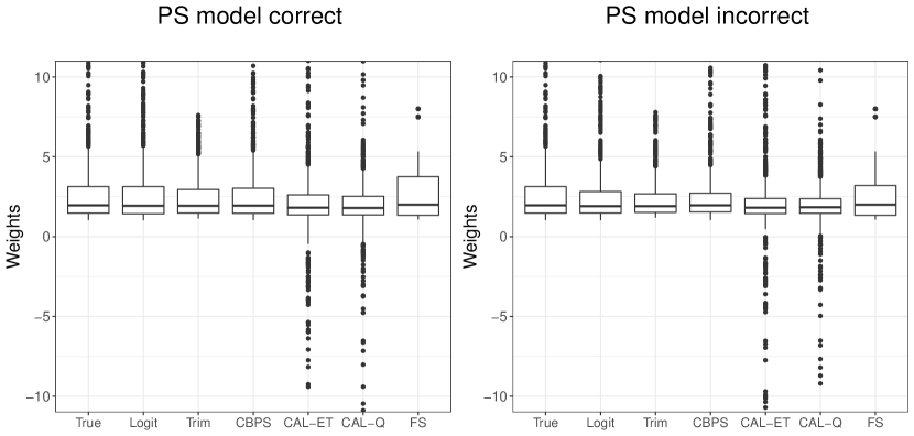
Figure 1: Distributions of weight estimates with various weighting scheme with a random simulated data set of sample size 1000. Weights outside the range of $[-10,10]$ are truncated; see also Figure S2 in the Supplementary Material for the full plot.

Table 2: Standardized imbalance measures of various weighting schemes under Chan et al., (2016)’s setting. We consider both correct ($\checkmark$) and incorrect ($\times$) specifications of the propensity score (PS) model*.

Sample size	Model		Weighting scheme
	PS		Logit	Trim	CBPS	CAL-ET	CAL-Q	FS
200	$\checkmark$		0.16	0.14	0.19	0.00	0.00	0.16
	$\times$		0.52	0.18	0.19	0.00	0.00	0.17
1000	$\checkmark$		0.07	0.06	0.09	0.00	0.00	0.07
	$\times$		0.70	0.08	0.11	0.00	0.00	0.08
5000	$\checkmark$		0.03	0.03	0.04	0.00	0.00	0.03
	$\times$		6.09	0.05	0.12	0.00	0.00	0.06

*: For the covariate balancing weighting schemes, we say the propensity score model is “correctly specified” if we impose balancing conditions on $\bm{X}$, and say the propensity score model is “misspecified” if we impose balancing conditions on $\bm{W}$.

As part of the design stage, we use Figure 1 and Figure S2 in the Supplementary Material to visualize the weight stability of various weighting schemes and Table 2 to assess the covariate balance after weighting. The covariate balance is measured using the standardized imbalance measure (Rosenbaum and Rubin,, 1985):

$$\text{Imb}=\Bigg{\{}\left(\dfrac{1}{N}\sum\limits_{i=1}^{N}\left[(Z_{i}w_{1i}-(1-Z_{i})w_{0i})\bm{X}_{i}\right]^{\top}\right)\left(\dfrac{1}{N}\sum\limits_{i=1}^{N}\bm{X}_{i}\bm{X}_{i}^{\top}\right)^{-1}\\ \times\left(\dfrac{1}{N}\sum\limits_{i=1}^{N}(Z_{i}w_{1i}-(1-Z_{i})w_{0i})\bm{X}_{i}\right)\Bigg{\}}^{1/2},$$

where $w_{1i}$ are weights for the treated and $w_{0i}$ are weights for the control. The logit weights perform reasonably well with a correctly specified propensity score model. However, with the misspecified propensity score model, they become highly unstable and cause severely imbalanced covariate distributions between the two treatment groups. The CAL weights may look very appealing as by design, they achieve exact balance in the standardized imbalance measure between the two treatment groups. However, as one can see from Figure 1 and Figure S2, they are highly unstable even under correct specification of the propensity score model. Consequently, the causal effect estimate may be driven by some highly influential observations. Moreover, the CAL weights can even be negative for many units. In contrast, the trimmed, CBPS and FS weights improve upon the logit weights in term of both stability and covariate balance, with trimmed and FS weights exhibiting uniformly better performance than CBPS weights. The performance of FS on covariate balance is particularly impressive as it does not (directly) target at achieving covariate balance between the two treatment groups.

Table 3: Bias and RMSE of classical weighting estimators with various weighting schemes under Chan et al., (2016)’s setting. We consider both correct ($\checkmark$) and incorrect ($\times$) specifications of the propensity score (PS) model* or the outcome regression (OR) model. The sample size is 1000.

Estimator	Model		Weighting scheme
	PS	OR	True	Logit	Trim	CBPS	CAL-ET	CAL-Q	FS
Bias
$\hat{\Delta}_{HT}$	$\checkmark$	$-$	-0.02	0.22	-0.12	-0.34	0.14	0.14	0.17
$\hat{\Delta}_{HT}$	$\times$	$-$	$-$	38.67	-4.20	9.91	0.07	1.80	0.02
$\hat{\Delta}_{Ratio}$	$\checkmark$	$-$	0.12	0.17	0.14	-0.18	0.14	0.14	0.17
$\hat{\Delta}_{Ratio}$	$\times$	$-$	$-$	6.62	-2.50	1.25	0.07	1.80	0.02
$\hat{\Delta}_{DR}$	$\checkmark$	$\checkmark$	0.14	0.14	-0.87	0.14	0.14	0.14	0.14
$\hat{\Delta}_{DR}$	$\checkmark$	$\times$	0.30	0.29	-0.85	0.57	1.67	2.97	0.43
$\hat{\Delta}_{DR}$	$\times$	$\checkmark$	$-$	0.14	-3.18	0.14	0.14	0.14	0.14
$\hat{\Delta}_{DR}$	$\times$	$\times$	$-$	-10.06	-4.27	-1.75	0.07	1.80	-0.78
RMSE
$\hat{\Delta}_{HT}$	$\checkmark$	$-$	16.98	7.76	5.09	6.67	1.72	1.72	2.09
$\hat{\Delta}_{HT}$	$\times$	$-$	$-$	136.54	6.78	12.61	1.91	2.62	2.01
$\hat{\Delta}_{Ratio}$	$\checkmark$	$-$	2.57	2.41	1.95	2.23	1.72	1.72	2.09
$\hat{\Delta}_{Ratio}$	$\times$	$-$	$-$	12.12	3.26	2.53	1.91	2.62	2.01
$\hat{\Delta}_{DR}$	$\checkmark$	$\checkmark$	1.72	1.72	1.80	1.72	1.72	1.72	1.72
$\hat{\Delta}_{DR}$	$\checkmark$	$\times$	2.23	2.18	1.89	2.11	2.47	3.50	2.16
$\hat{\Delta}_{DR}$	$\times$	$\checkmark$	$-$	1.74	3.57	1.72	1.72	1.72	1.72
$\hat{\Delta}_{DR}$	$\times$	$\times$	$-$	53.24	4.59	2.93	1.91	2.62	2.07

*: For the covariate balancing weighting schemes, we say the propensity score model is “correctly specified” if we impose balancing conditions on $\bm{X}$, and say the propensity score model is “misspecified” if we impose balancing conditions on $\bm{W}$.

Table 3 summarizes the performance of various weighting schemes when they are applied to the three classical weighting estimators. For brevity, we only show results with sample size fixed at 1000. Consistent with the findings of Kang and Schafer, (2007), logit weights are sensitive to misspecification of the propensity score model, regardless of whether the weighting estimator is doubly robust or not. Use of the full subclassification weights or the covariate balancing weights (CBPS, CAL-ET and CAL-Q) greatly improves upon the naive weights obtained from a logistic regression model. Among them, FS, CAL-ET and CAL-Q weights perform better than CBPS weights under most simulation settings, and the IPW estimator coincides with the Ratio estimator with the FS, CAL-ET and CAL-Q weights. One noticeable exception is the scenario where the propensity score model is correctly specified while the outcome regression model is misspecified. In this case, when combined with $\hat{\Delta}_{DR},$ CAL-ET and CAL-Q produce estimates with large bias. This is not surprising as neither of these two estimators relies on an explicit propensity score model, so unlike CBPS and FS, their performance does not directly benefit from correct specification of the propensity score model. From Table 3, one can also see that the proposed FS weights outperform the trimmed weights. This suggests that the FS weights improve upon the logit weights beyond stabilizing the extreme weights.

Figure 2 presents results on interval estimates. Following Theorem 4, we consider the setting where both conditions (i) and (ii) hold. We compare interval estimates based on two variance estimators: $\hat{\sigma}_{dr}^{2}$ described in Theorem 4, and the variance estimator based on 1000 non-parametric bootstrap samples. The left panel in Figure 2 shows that estimates from the corresponding standard deviation estimators are close to the Monte Carlo standard deviation, and decrease with the sample size at approximately the root-N rate. The right panel in Figure 2 shows the empirical coverage probability of the 95% Wald-type confidence intervals constructed based on the two variance estimators. Both of these confidence intervals have approximately the nominal coverage level as the sample size increases.

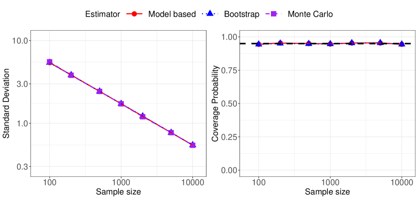
Figure 2: Performance of model-based variance estimator for $\hat{\Delta}_{DR}^{S}.$ The black dashed line on the right panel shows the 95% nominal coverage level.

5 Application to a childhood nutrition study

We illustrate the application of the proposed full subclassification weighting method using data from the 2007-2008 National Health and Nutrition Examination Survey (NHANES), which is a program of studies designed to assess the health and nutritional status of adults and children in the United States. The data set we use was created by Chan et al., (2016), which contained observations on 2330 children aged from 4 to 17. Of these children, 55.1% participated in the National School Lunch or the School Breakfast programs. These were federally funded meal programs primarily designed to provide meals for children from poor neighborhoods in the United States. However, there have been concerns that meals provided through these programs may cause childhood obesity (Stallings et al.,, 2010). Hence here we study how participation in these meal programs contributes to childhood obesity as measured by body mass index (BMI). We control for the same set of potential confounders in our analysis as Chan et al., (2016); see the Supplementary Material for a detailed list.

Table S1 in the Supplementary Material summarizes baseline characteristics and outcome measure by participation status in the school meal programs. Children participating in the school meal programs are more likely to be black or Hispanic, and come from a family with lower social economic status. Respondents for such children also tend to be younger and female. These differences in baseline characteristics suggest that the observed mean difference in BMI, that is 0.53 $kg/m^{2}$ (95% CI (0.11, 0.96)), may not be fully attributable to the school meal programs.

We then apply various weighting methods to estimate the effect of participation in the meal programs. We consider two models for the propensity score: a logistic model and a complementary log-log model. We also consider a linear outcome regression model on the log-transformed BMI. All the covariates enter the propensity score model or the outcome regression model as linear terms. Figure 3 visualizes the distributions of propensity score weights and their reciprocals. Results with the complementary log-log propensity score model are similar to those with the logistic regression model and are omitted. We can see that the reciprocals of propensity score weights estimated using the full subclassification method or the CBPS method lie within the unit interval. In contrast, the reciprocals of CAL weights can be negative or greater than 1. Hence these weights cannot be interpreted as propensity scores. Furthermore, consistent with our findings in Figures 1 and S2, the CAL weights are much more dispersed than other weights. The five most extreme weights estimated by CAL-ET are $1350,1259,-959,-943,677$, and those for CAL-Q are $324,153,-97,-97,85.$ As these weights are obtained independently of the outcome data, the final causal estimates are highly sensitive to these outliers.

Table 4 summarizes the standardized imbalance measure and causal effect estimates. As advocated by Rubin, (2007), the construction of propensity score weights should make the final causal effect estimate insensitive to the weighting estimator used. However, the propensity score weights estimated with a parametric model or the CBPS method tend to give different answers with different weighting estimators. With these weighting methods, a Horvitz-Thompson estimator would suggest that participation in the school meal programs led to a significantly lower BMI. The Ratio estimator and DR estimator instead yield estimates that are much closer to zero. In contrast, the trimmed weights, the subclassification weights (both the classical ones and the FS weights), and the CAL weights have a consistent implication with different weighting estimators that participation in school meal programs have negligible effects on the BMI. Moreover, although different parametric propensity score models may give rise to very different causal effect estimates with a Horvitz-Thompson estimator, they yield much closer estimates with a (full) subclassification estimator. These results show that the subclassification methods are robust against propensity score model misspecification.

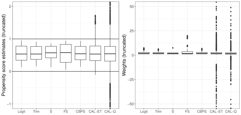
Figure 3: Distributions of propensity score estimates and weights with the NHANES data.

Table 4: The average causal effect estimates associated with participation in the school meal programs. The 95% Wald-type confidence intervals in brackets are computed based on bootstrap estimates.

	Imbalance	HT	Ratio	DR
Naive*	1.04	0.53 (0.11,0.96)	0.53 (0.11,0.96)	0.10 (-0.21,0.42)
Logit	0.10	-1.52 (-2.46,-0.58)	-0.16 (-0.64,0.32)	0.08 (-0.38,0.54)
Trim	0.06	-0.01 (-1.09,1.06)	-0.00 (-0.53,0.53)	0.09 (-0.35,0.52)
S	0.08	-0.12 (-0.61,0.38)	-0.12 (-0.61,0.38)	-0.02 (-0.48,0.44)
FS	0.12	-0.20 (-0.75,0.36)	-0.20 (-0.75,0.36)	-0.10 (-0.60,0.40)
Cloglog**	0.15	-2.26 (-3.67,-0.85)	-0.23 (-0.76,0.30)	0.14 (-0.35,0.63)
Trim $\plus$ Cloglog	0.13	0.70 (-0.48,1.88)	0.20 (-0.33,0.73)	0.17 (-0.26,0.60)
S $\plus$ Cloglog	0.16	-0.05 (-0.55,0.44)	-0.05 (-0.55,0.44)	0.01 (-0.45,0.47)
FS $\plus$ Cloglog	0.14	0.01 (-0.57,0.59)	0.01 (-0.57,0.59)	0.08 (-0.43,0.60)
CBPS	0.10	-1.25 (-2.11,-0.40)	-0.05 (-0.49,0.39)	0.07 (-0.35,0.50)
CAL-ET	0.00	-0.05 (-0.48,0.39)	-0.05 (-0.48,0.39)	0.07 (-0.36,0.51)
CAL-Q	0.00	-0.02 (-0.45,0.42)	-0.02 (-0.45,0.42)	0.10 (-0.34,0.53)

*: “Naive” corresponds to the crude estimator not adjusting for any confounders;
**: Cloglog indicates that the propensity scores are estimated with a complementary log-log model.

6 Discussion

Propensity score weighting is among the most popular tools for drawing causal inference in various contexts. However, with parametric specification of the propensity score model, propensity score weighting estimators tend to be very sensitive to model misspecification. In this paper, we investigate robust estimation of propensity score weights, along the line of research by Hainmueller, (2012); Imai and Ratkovic, (2014); Zubizarreta, (2015); Chan et al., (2016). Specifically, we propose a novel (full) subclassification scheme that only exploits the rank information from the parametric model-based propensity score estimates, and thus improving upon robustness to model misspecification. As discussed in detail by Zubizarreta, (2015), a covariate balance-stability trade-off is key to constructing robust propensity score weights. Through extensive empirical studies, we show that the full subclassification weighting method achieves a good compromise in this trade-off, and dramatically improves upon model-based propensity score weights in both aspects, especially when the propensity score model is misspecified.

Our approach in this paper is based on subclassification by the quantiles of the estimated propensity scores. It is an interesting area for subsequent research to consider alternative ways of forming subclasses and providing theoretical justifications for these alternative approaches. We refer interested readers to Myers and Louis, (2007) for an earlier investigation along these lines.

We have focused our illustration on causal estimation from observational studies. Since the full subclassification weights are constructed independently of the outcome data, it can potentially be applied to improve propensity score estimation in other contexts, such as addressing the missing data problem under the missing at random (MAR) assumption (see e.g., Rubin,, 1978; Gelman and Meng,, 2004; Kang and Schafer,, 2007), causal inference with a marginal structural model (Robins et al.,, 2000) and in presence of interference (Tchetgen Tchetgen and VanderWeele,, 2012). It can also be extended to obtain robust estimates of the generalized propensity score with multi-arm treatments (Imbens,, 2000; Imai and Van Dyk,, 2004).

SUPPLEMENTARY MATERIALS FOR

“ROBUST ESTIMATION OF PROPENSITY SCORE WEIGHTS

VIA SUBCLASSIFICATION”

¹Linbo Wang, ²Yuexia Zhang, ³Thomas S. Richardson, ⁴Xiao-Hua Zhou

^1,2University of Toronto, ³University of Washington, ⁴Peking University

S1 Proof of Proposition 1

The proof is straightforward by noting that

$$\sum\limits_{i=1}^{N}Z_{i}/\hat{p}_{\hat{k}_{i}}=\sum\limits_{i=1}^{N}n_{\hat{k}_{i}}Z_{i}/n_{1\hat{k}_{i}}=\sum\limits_{k=1}^{K}\left\{(n_{k}/n_{1k})\sum\limits_{i:\hat{k}_{i}=k}Z_{i}\right\}=\sum\limits_{k=1}^{K}\left\{(n_{k}/n_{1k})n_{1k}\right\}=N,$$

and similarly

$$\sum\limits_{i=1}^{N}(1-Z_{i})/(1-\hat{p}_{\hat{k}_{i}})=N.$$

S2 Regularity conditions for Theorem 1

We now introduce the regularity conditions that will be used for proving (root-N) consistency of $\hat{\Delta}_{HT}^{S}$.

Assumption S2

(Compact set) The parameter $\Delta$ lies in the interior of a compact set $\mathscr{A}$; $\beta$ lies in the interior of a compact set $\mathscr{B}$.

Assumption S3

(Uniform positivity) (i) The support of $\pi(\bm{X};\beta)$ can be written as $[\pi_{min},\pi_{max}]$, where $\pi_{min}>0,\pi_{max}<1$, and the quantile distribution of $\pi(\bm{X};\beta)$ is Lipschitz continuous. (ii) There exist constants $c_{1}$ and $c_{2}$ such that $0<c_{1}<\pi(\bm{X};\bar{\beta})<c_{2}<1$ almost surely for all $\bar{\beta}\in\mathscr{B}$.

Assumption S3 (i) implies that the cumulative distribution function of $\pi(\bm{X};\beta)$ has no flat portions between $[\pi_{min},\pi_{max}]$, or the quantile distribution of $\pi(\bm{X};\beta)$ is continuous on $[0,1]$. Violation of this assumption will cause some subclasses to be always empty, and the subclassification estimator to be ill-defined. This problem may be solved by considering only non-empty subclasses in constructing the subclassification estimator. For simplicity, we do not get into discussion of this issue here.

Assumption S4

(Uniform consistency of estimated propensity scores) The propensity score model is correctly specified such that for all $N,\hat{\pi}_{i}\ (i=1,\ldots,N)$ is uniformly convergent in probability to $\pi_{i}\ (i=1,\ldots,N)$ at $\sqrt{N}$ rate, where $\hat{\pi}_{i}=\hat{\pi}(\bm{X}_{i})$ and $\pi_{i}=\pi(\bm{X}_{i};\beta)$. Formally, $\sqrt{N}\max\limits_{1\leq i\leq N}|\hat{\pi}_{i}-\pi_{i}|=O_{p}(1)$.

Under a smooth parametric model, the uniformity part in Assumptions S3 and S4 can usually be inferred from uniform boundedness of the maximum norm of covariates, $|\bm{X}_{i}|_{\infty}$ $(i=1,\ldots,N)$. The latter assumption holds if the support of the covariate $\bm{X}$ is a bounded set in $\mathbb{R}^{p}$, where $p$ is the dimension of $\bm{X}$. This assumption has been widely used in the causal inference literature (for example, see Hirano et al.,, 2003).

As an illustration, suppose the true propensity score model is a logistic regression model:

$$\pi(\bm{X};\beta)=\text{expit}(\bm{X}^{\top}\beta)=\dfrac{\text{exp}(\bm{X}^{\top}\beta)}{1+\text{exp}(\bm{X}^{\top}\beta)}.$$

In this case, $\pi(\bm{X}_{i};\beta)$ is uniformly bounded away from 0 and 1 if $|\bm{X}_{i}|_{\infty}\ (i=1,\ldots,N)$ are uniformly bounded. At the same time, by the mean value theorem,

$$\sqrt{N}\left|\hat{\pi}(\bm{X}_{i})-\pi(\bm{X}_{i};\beta)\right| =\sqrt{N}\left|\text{expit}(\bm{X}_{i}^{\top}\tilde{\beta})\{1-\text{expit}(\bm{X}_{i}^{\top}\tilde{\beta})\}\bm{X}_{i}^{\top}(\hat{\beta}-\beta)\right|$$

$$\leq\sqrt{N}\|\bm{X}_{i}\|_{\infty}\|\hat{\beta}-\beta\|_{\infty},$$

where $\hat{\beta}$ is a consistent estimator of $\beta$, and $\tilde{\beta}$ lies between $\hat{\beta}$ and $\beta$. Hence $\hat{\pi}(\bm{X}_{i})-\pi(\bm{X}_{i};\beta)\ (i=1,\ldots,N)$ is uniformly convergent in probability to zero at $\sqrt{N}$ rate if $|\bm{X}_{i}|_{\infty}\ (i=1,\ldots,N)$ are uniformly bounded.

Assumption S5

(Smoothness of propensity score model) $\pi(\bm{X};\beta)$, $\partial\pi(\bm{X};\beta)/\partial\beta$ and $\partial^{2}\pi(\bm{X};\beta)/\partial\beta\partial\beta^{\top}$ are continuous functions of $\beta$.

Assumption S6

(Finite second moments) $E(Y^{2})<\infty$ and $E\|\partial\pi(\bm{X};\beta)/\partial\beta\|^{2}<\infty$, where $\|\cdot\|$ denotes the Euclidean norm.

Assumptions S5 and S6 are standard regularity conditions in the M-estimation theory.

Assumption S7

(Weak correlation between subclasses) $\max\limits_{k,j\in\{1,\ldots,K\},k\neq j}\big{|}\text{cov}(n_{1k},n_{1j}\mid I(\hat{\pi}_{i}\in\hat{C}_{\ell}),i=1,\ldots,N,\ell=1,\ldots,K)\big{|}=O_{p}(N/K^{2})$.

If one employs a sampling splitting procedure in which separate samples are used for constructing the subclasses, and estimating the average treatment effect, then $n_{1k}\Large\mbox{$\perp\kern-5.5pt\perp$}n_{1j}\mid I(\hat{\pi}_{i}\in\hat{C}_{\ell}),i=1,\ldots,N,\ell=1,\ldots,K$. In this case, Assumption S7 holds trivially.

S3 Proof of Theorem 1

Under Assumptions S1–S5, it can be proved using the standard M-estimation theory that

$$\sqrt{N}(\hat{\Delta}_{HT}-\Delta)\rightarrow_{d}N(0,\Sigma_{HT}),$$

where $\Sigma_{HT}$ is computed in Lunceford and Davidian, (2004). To prove Theorem 1, we connect $\hat{\Delta}_{HT}^{S}$ and $\hat{\Delta}_{HT}$ with an intermediate (infeasible) estimator $\hat{\Delta}_{S-HT}$:

$$\hat{\Delta}_{S-HT}=\sum\limits_{k=1}^{K}\left\{\dfrac{1}{N{p_{k}}}\sum\limits_{i=1}^{N}Z_{i}Y_{i}I(\hat{\pi}_{i}\in\hat{C}_{k})-\dfrac{1}{N(1-{p_{k}})}\sum\limits_{i=1}^{N}(1-Z_{i})Y_{i}I(\hat{\pi}_{i}\in\hat{C}_{k})\right\},$$

where $p_{k}=pr(Z=1\mid\hat{\pi}_{i}\in\hat{C}_{k}).$

In the first step, Lemma 6 shows that the difference between $\hat{\Delta}_{S-HT}$ and $\hat{\Delta}_{HT}$ tends to zero. We defer the proof of Lemma 6 to the end of this section. In the second step, we show that the difference between $\hat{\Delta}_{HT}^{S}$ and $\hat{\Delta}_{S-HT}$ tends to zero.

Lemma 6

Under Assumption 1, the regularity conditions in the Supplementary Material, and condition (3.4),

• $\hat{\Delta}_{S-HT}$ is consistent for estimating $\Delta$: $\hat{\Delta}_{S-HT}-\Delta=o_{p}(1);$

• If we assume additionally that (3.5) holds, then $\hat{\Delta}_{S-HT}$ is $\sqrt{N}$-consistent for estimating $\Delta$: $\sqrt{N}(\hat{\Delta}_{S-HT}-\Delta)=O_{p}(1).$

We now turn to the second step, in which we show that under (3.5),

$$\sqrt{N}(\hat{\Delta}_{HT}^{S}-\hat{\Delta}_{S-HT})=O_{p}(1).$$ (S3.1)

By symmetry, we only show (S3.1) for the active treatment group, i.e.

$$\sqrt{N}\sum\limits_{k=1}^{K}\dfrac{n_{k}}{N}\left\{\left(1-\dfrac{n_{1k}}{n_{k}p_{k}}\right)\dfrac{1}{n_{1k}}\sum\limits_{i=1}^{N}Z_{i}Y_{i}I(\hat{\pi}_{i}\in\hat{C}_{k})\right\}=O_{p}(1),$$ (S3.2)

where $K$ is used as a shorthand for $K(N)$.

Without loss of generality, we assume $n_{1}=\cdots=n_{K}=N/K\triangleq n$. As $\hat{\Delta}_{HT}^{S}$ is well-defined, $n_{1k}\notin\{0,n\},k=1,\ldots,K$. Thus $n_{1k}\sim tBin(n,p_{k})$, where $tBin$ denotes truncated binomial distribution with range $[1,n-1]$.

We will use Markov’s inequality to show (S3.2). Denote

$$h_{k} =\dfrac{1-p_{k}^{n-1}}{1-p_{k}^{n}-(1-p_{k})^{n}}-\dfrac{n_{1k}}{np_{k}}=c_{Nk}-\dfrac{n_{1k}}{np_{k}}\quad\text{ (note }E[h_{k}]=0);$$

$$m_{1k} =\dfrac{1}{n_{1k}}\sum\limits_{i=1}^{N}Z_{i}Y_{i}I(\hat{\pi}_{i}\in\hat{C}_{k});$$

$$S_{NK} =\dfrac{1}{K}\sum\limits_{k=1}^{K}h_{k}m_{1k}.$$

Then the left hand side of (S3.2) can be written as

$$\sqrt{N}\sum\limits_{k=1}^{K}\dfrac{n}{N}\left\{\left(1-c_{Nk}\right)\dfrac{1}{n_{1k}}\sum\limits_{i=1}^{N}Z_{i}Y_{i}I(\hat{\pi}_{i}\in\hat{C}_{k})\right\}$$ (S3.3)

$$+\sqrt{N}\sum\limits_{k=1}^{K}\dfrac{n}{N}\left\{\left(c_{Nk}-\dfrac{n_{1k}}{np_{k}}\right)\dfrac{1}{n_{1k}}\sum\limits_{i=1}^{N}Z_{i}Y_{i}I(\hat{\pi}_{i}\in\hat{C}_{k})\right\}$$

$$= \dfrac{\sqrt{N}}{K}\sum\limits_{k=1}^{K}(1-c_{Nk})m_{1k}+\sqrt{N}S_{NK}.$$

We shall show that

$$\dfrac{\sqrt{N}}{K}\sum\limits_{k=1}^{K}(1-c_{Nk})m_{1k}=o_{p}(1),$$ (S3.4)

and

$$\sqrt{N}S_{NK}=O_{p}(1).$$ (S3.5)

Let $\pi_{thres}=\min\{\pi_{min}/2,(1-\pi_{max})/2\}$. Note that equation (S4.16) (see the proof of Lemma 6) implies $c_{Nk}-1=\{p_{k}^{n}-p_{k}^{n-1}+(1-p_{k})^{n}\}/\{1-p_{k}^{n}-(1-p_{k})^{n}\}=O((1-\pi_{thres})^{n})$. Moreover, by symmetry, we have

$$E(m_{1k}^{2}\mid n_{1k}) =\mu_{1k}^{12}+a_{2}\dfrac{1}{n_{1k}},$$

where $a_{2}=\mu_{1k}^{11}-\mu_{1k}^{12}$ with $\mu_{1k}^{11}=E\{Y_{1}^{2}\mid Z_{1}I(\hat{\pi}_{1}\in\hat{C}_{k})=1\}$ and $\mu_{1k}^{12}=E\{Y_{1}Y_{2}\mid Z_{1}I(\hat{\pi}_{1}\in\hat{C}_{k})Z_{2}I(\hat{\pi}_{2}\in\hat{C}_{k})=1\}$. Furthermore,

$$E(m_{1k}^{2})=E\left(\mu_{1k}^{12}+a_{2}\dfrac{1}{n_{1k}}\right)=\mu_{1k}^{12}+a_{2}\left\{\dfrac{np_{k}}{(np_{k}+r_{k})^{2}}+O\left(\dfrac{1}{n^{2}}\right)\right\},$$

where $r_{k}=1-p_{k}$, and we use the fact that $E(1/n_{1k})=np_{k}/\{(np_{k}+r_{k})^{2}\}+O(1/n^{2})$ (Znidaric,, 2005). According to Assumption S5, $\mu_{1k}^{12}=O(1)$ and $a_{2}=O(1)$. Thus, $E(m_{1k}^{2})=O(1)$. Based on the Markov’s inequality, we have $m_{1k}=O_{p}(1)$. If Assumptions (3.5) and (3.6) are also satisfied, then $\sqrt{N}\max_{1\leq k\leq K}|(1-c_{Nk})m_{1k}|=\sqrt{N}O((1-\pi_{thres})^{n})O_{p}(1)=o_{p}(1)$. Since $\sqrt{N}/{K}\sum_{k=1}^{K}(1-c_{Nk})m_{1k}\leq\sqrt{N}\max_{1\leq k\leq K}|(1-c_{Nk})m_{1k}|$, then (S3.4) holds.

Note that

$$E(NS_{NK}^{2})=E\dfrac{N}{K^{2}}\left(\sum\limits_{k=1}^{K}h_{k}m_{1k}\right)^{2}=\dfrac{N}{K^{2}}\left\{\sum_{k=1}^{K}E(h_{k}^{2}m_{1k}^{2})+\sum_{k\neq j}E(h_{k}m_{1k}h_{j}m_{1j})\right\}.$$ (S3.6)

Under Assumptions S5, (3.5) and (3.6),

$$\max\limits_{1\leq k\leq K}E(h_{k}^{2}m_{1k}^{2})= \max\limits_{1\leq k\leq K}E\{E(h_{k}^{2}m_{1k}^{2}\mid n_{1k})\}$$ (S3.7)

$$= \max\limits_{1\leq k\leq K}E\{h_{k}^{2}E(m_{1k}^{2}\mid n_{1k})\}$$

$$= \max\limits_{1\leq k\leq K}E\left\{h_{k}^{2}\left(\mu_{1k}^{12}+a_{2}\dfrac{1}{n_{1k}}\right)\right\}$$

$$= \max\limits_{1\leq k\leq K}\left\{\mu_{1k}^{12}E\left(c_{Nk}^{2}-\dfrac{2c_{Nk}n_{1k}}{np_{k}}+\dfrac{n_{1k}^{2}}{n^{2}p_{k}^{2}}\right)+a_{2}E\left(\dfrac{c_{Nk}^{2}}{n_{1k}}-\dfrac{2c_{Nk}}{np_{k}}+\dfrac{n_{1k}}{n^{2}p_{k}^{2}}\right)\right\}$$

$$= \max\limits_{1\leq k\leq K}\Bigg{[}\mu_{1k}^{12}\left\{c_{Nk}^{2}-2c_{Nk}^{2}+\dfrac{(n^{2}p_{k}^{2}+np_{k}-np_{k}^{2}-n^{2}p_{k}^{n})c_{Nk}}{(1-p_{k}^{n-1})n^{2}p_{k}^{2}}\right\}$$

$$\qquad\quad+a_{2}\left[c_{Nk}^{2}\left\{\dfrac{np_{k}}{(np_{k}+r_{k})^{2}}+O\left(\dfrac{1}{n^{2}}\right)\right\}-\dfrac{2c_{Nk}}{np_{k}}+\dfrac{c_{Nk}}{np_{k}}\right]\Bigg{]}$$

$$= \max\limits_{1\leq k\leq K}\Bigg{[}\left\{\dfrac{\mu_{1k}^{12}(n^{2}p_{k}^{2}+np_{k}-np_{k}^{2}-n^{2}p_{k}^{n})}{(1-p_{k}^{n-1})n^{2}p_{k}^{2}}-\dfrac{(\mu_{1k}^{11}-\mu_{1k}^{12})}{np_{k}}\right\}c_{Nk}$$

$$\qquad\quad+\left\{(\mu_{1k}^{11}-\mu_{1k}^{12})\dfrac{np_{k}}{(np_{k}+r_{k})^{2}}-\mu_{1k}^{12}\right\}c_{Nk}^{2}+O\left(\dfrac{1}{n^{2}}\right)\Bigg{]}$$

$$= O\left(\dfrac{1}{n}\right)+O\left(\dfrac{1}{n^{2}}\right)=O\left(\dfrac{1}{n}\right),$$

where the last equality holds because $p_{k}$ is bounded away from 0 and 1. Moreover,

$$\max\limits_{k,j\in\{1,\ldots,K\},k\neq j}E(h_{k}m_{1k}h_{j}m_{1j})$$ (S3.8)

$$= \max\limits_{k,j\in\{1,\ldots,K\},k\neq j}E\{E(h_{k}m_{1k}h_{j}m_{1j}\mid n_{1k},n_{1j})\}$$

$$= \max\limits_{k,j\in\{1,\ldots,K\},k\neq j}E\{h_{k}h_{j}E(m_{1k}m_{1j}\mid n_{1k},n_{1j})\}$$

$$= \max\limits_{k,j\in\{1,\ldots,K\},k\neq j}E\left[h_{k}h_{j}E\left\{\dfrac{1}{n_{1k}}\sum\limits_{i=1}^{N}Z_{i}Y_{i}I(\hat{\pi}_{i}\in\hat{C}_{k})\dfrac{1}{n_{1j}}\sum\limits_{i=1}^{N}Z_{i}Y_{i}I(\hat{\pi}_{i}\in\hat{C}_{j})\big{\mid}n_{1k},n_{1j}\right\}\right]$$

$$= \max\limits_{k,j\in\{1,\ldots,K\},k\neq j}E\left[h_{k}h_{j}E\left\{Y_{1}Y_{2}\big{\mid}Z_{1}I(\hat{\pi}_{1}\in\hat{C}_{k})Z_{2}I(\hat{\pi}_{2}\in\hat{C}_{j})=1\right\}\right]\text{ (by symmetry)}$$

$$= \max\limits_{k,j\in\{1,\ldots,K\},k\neq j}E\left\{\left(c_{Nk}-\dfrac{n_{1k}}{np_{k}}\right)\left(c_{Nj}-\dfrac{n_{1j}}{np_{j}}\right)\right\}E\left\{Y_{1}Y_{2}\big{\mid}Z_{1}I(\hat{\pi}_{1}\in\hat{C}_{k})Z_{2}I(\hat{\pi}_{2}\in\hat{C}_{j})=1\right\}$$

$$= \max\limits_{k,j\in\{1,\ldots,K\},k\neq j}\frac{1}{n^{2}p_{k}p_{j}}\left\{E(n_{1k}n_{1j})-E(n_{1k})E(n_{1j})\right\}E\left\{Y_{1}Y_{2}\big{\mid}Z_{1}I(\hat{\pi}_{1}\in\hat{C}_{k})Z_{2}I(\hat{\pi}_{2}\in\hat{C}_{j})=1\right\}$$

$$= \max\limits_{k,j\in\{1,\ldots,K\},k\neq j}\frac{1}{n^{2}p_{k}p_{j}}\text{cov}(n_{1k},n_{1j})E\left\{Y_{1}Y_{2}\big{\mid}Z_{1}I(\hat{\pi}_{1}\in\hat{C}_{k})Z_{2}I(\hat{\pi}_{2}\in\hat{C}_{j})=1\right\}$$

$$= \max\limits_{k,j\in\{1,\ldots,K\},k\neq j}\Bigg{[}\frac{1}{n^{2}p_{k}p_{j}}\Big{[}E\{\text{cov}(n_{1k},n_{1j}\mid I(\hat{\pi}_{i}\in\hat{C}_{\ell}),i=1,\ldots,N,\ell=1,\ldots,K)\}$$

$$\!+\!\text{cov}\left\{E\left(n_{1k}\!\mid\!I(\hat{\pi}_{i}\in\hat{C}_{\ell}),i=1,\ldots,N,\ell=1,\ldots,K\right),E(n_{1j}\!\mid\!I(\hat{\pi}_{i}\in\hat{C}_{\ell}),i=1,\ldots,N,\ell=1,\ldots,K)\right\}\Big{]}$$

$$\qquad\qquad\qquad\times E\left\{Y_{1}Y_{2}\big{\mid}Z_{1}I(\hat{\pi}_{1}\in\hat{C}_{k})Z_{2}I(\hat{\pi}_{2}\in\hat{C}_{j})=1\right\}\Bigg{]}$$

$$= \max\limits_{k,j\in\{1,\ldots,K\},k\neq j}\Bigg{[}\frac{1}{n^{2}p_{k}p_{j}}E\{\text{cov}(n_{1k},n_{1j}\mid I(\hat{\pi}_{i}\in\hat{C}_{\ell}),i=1,\ldots,N,\ell=1,\ldots,K)\}$$

$$\qquad\qquad\qquad\times E\left\{Y_{1}Y_{2}\big{\mid}Z_{1}I(\hat{\pi}_{1}\in\hat{C}_{k})Z_{2}I(\hat{\pi}_{2}\in\hat{C}_{j})=1\right\}\Bigg{]}$$

$$\leq \max\limits_{k,j\in\{1,\ldots,K\},k\neq j}\left[\frac{1}{n^{2}p_{k}p_{j}}\Big{|}E\left\{Y_{1}Y_{2}\big{\mid}Z_{1}I(\hat{\pi}_{1}\in\hat{C}_{k})Z_{2}I(\hat{\pi}_{2}\in\hat{C}_{j})=1\right\}\Big{|}\right]$$

$$\times E\left\{\max\limits_{k,j\in\{1,\ldots,K\},k\neq j}\Big{|}\text{cov}(n_{1k},n_{1j}\mid I(\hat{\pi}_{i}\in\hat{C}_{\ell}),i=1,\ldots,N,\ell=1,\ldots,K)\Big{|}\right\}.$$

Under Assumption S5, we have $\big{|}E\left\{Y_{1}Y_{2}\big{\mid}Z_{1}I(\hat{\pi}_{1}\in\hat{C}_{k})Z_{2}I(\hat{\pi}_{2}\in\hat{C}_{j})=1\right\}\big{|}=O(1)$. Combined with Assumption S6, we then get that

$$\max_{k,j\in\{1,\ldots,K\},k\neq j}E(h_{k}m_{1k}h_{j}m_{1j})=O(1/N).$$ (S3.9)

Equations (S3.6), (S3.7) and (S3.9) together imply that $E(NS_{NK}^{2})=O(1)$. Based on the Markov’s inequality, we can get (S3.5).

We have hence finished the proof.

S4 Proof of Lemma 6

For simplicity we only prove claim (ii). Proof of claim (i) can be obtained following similar arguments. Due to the asymptotic normality of $\hat{\Delta}_{HT}$, it suffices to show that

$$\sqrt{N}(\hat{\Delta}_{S-HT}-\hat{\Delta}_{HT})=O_{p}(1).$$

Let $\pi_{1},\ldots,\pi_{n}$ be independent samples of $\pi(\bm{X};\beta)$, and $F^{-1}(\cdot)$ be the quantile distribution of $\pi(\bm{X};\beta)$. For $t\in(0,1)$, the empirical quantile distribution is defined as

$$\mathbb{F}_{N}^{-1}(t)=\inf\left\{x:\mathbb{F}_{N}(x)\geq t\right\},$$

where $\mathbb{F}_{N}(x)=\sum_{i=1}^{N}1_{(-\infty,x]}(\pi_{i})/N$ is the empirical distribution function.

Using standard empirical process theory (Shorack and Wellner,, 1986), we can show that

$$\sqrt{N}\|\mathbb{F}_{N}^{-1}-F^{-1}\|_{0}^{1}=\sqrt{N}\sup\limits_{0\leq t\leq 1}|\mathbb{F}_{N}^{-1}(t)-F^{-1}(t)|=O_{p}(1).$$ (S4.10)

As $F^{-1}(t)$ is Lipschitz continuous,

$$K\max\limits_{1\leq k\leq K}\{q_{k}-q_{k-1}\}=O(1),$$ (S4.11)

where $q_{k}=F^{-1}\left(k/K\right)$. Assumption (3.5), results (S4.10) and (S4.11) together imply

$$\sqrt{N}\max\limits_{1\leq k\leq K}|\tilde{q}_{k}-q_{k}|=O_{p}(1)\text{\quad and \quad}\sqrt{N}\max\limits_{1\leq k\leq K}\{\tilde{q}_{k}-\tilde{q}_{k-1}\}=O_{p}(1),$$ (S4.12)

where $\tilde{q}_{k}=\mathbb{F}_{N}^{-1}\left(k/K\right)\ (k=1,\ldots,K)$, the sample quantiles of the (true) propensity scores. Now let $\hat{q}_{k}$ be the sample quantiles of the estimated propensity scores, Assumptions (3.5) and S4, and result (S4.12) imply

$$\sqrt{N}\max\limits_{1\leq k\leq K}|\hat{q}_{k}-q_{k}|=O_{p}(1)\text{\quad and \quad}\sqrt{N}\max\limits_{1\leq k\leq K}\{\hat{q}_{k}-\hat{q}_{k-1}\}=O_{p}(1).$$ (S4.13)

Denote $\hat{\pi}_{min}=\min\{\hat{\pi}_{i},i=1,\ldots,N\}$, $\hat{\pi}_{max}=\max\{\hat{\pi}_{i},i=1,\ldots,N\}$ and $\pi_{thres}=\min\{\pi_{min}/2,(1-\pi_{max})/2\}$, Assumptions S3 and S4 imply that for large enough $N$,

$$\pi_{thres}<\min(\hat{\pi}_{min},1-\hat{\pi}_{max}).$$ (S4.14)

Moreover, if we let $\delta=\max_{1\leq i\leq N}|\hat{\pi}_{i}-\pi_{i}|$, then

$$p_{\hat{k}_{i}} =P(Z=1\mid\hat{\pi}_{i}\in[\hat{q}_{\hat{k}_{i}-1},\hat{q}_{\hat{k}_{i}}])$$

$$=E_{\pi_{i}\mid\hat{\pi}_{i}\in[\hat{q}_{\hat{k}_{i}-1},\hat{q}_{\hat{k}_{i}}]}E\left\{P(Z=1\mid\pi_{i},\hat{\pi}_{i}\in[\hat{q}_{\hat{k}_{i}-1},\hat{q}_{\hat{k}_{i}}])\mid\hat{\pi}_{i}\in[\hat{q}_{\hat{k}_{i}-1},\hat{q}_{\hat{k}_{i}}]\right\}$$

$$=E_{\pi_{i}\mid\hat{\pi}_{i}\in[\hat{q}_{\hat{k}_{i}-1},\hat{q}_{\hat{k}_{i}}]}E\left\{\pi_{i}\mid\hat{\pi}_{i}\in[\hat{q}_{\hat{k}_{i}-1},\hat{q}_{\hat{k}_{i}}]\right\}$$

$$\in[\hat{q}_{\hat{k}_{i}-1}-\delta,\hat{q}_{\hat{k}_{i}}+\delta].$$

On the other hand, $\hat{\pi}_{i}\in[\hat{q}_{\hat{k}_{i}-1},\hat{q}_{\hat{k}_{i}}]\subset[\hat{q}_{\hat{k}_{i}-1}-\delta,\hat{q}_{\hat{k}_{i}}+\delta]$, hence

$$|p_{\hat{k}_{i}}-\hat{\pi}_{i}|\leq\max\limits_{1\leq k\leq K}\{\hat{q}_{k}-\hat{q}_{k-1}\}+2\max\limits_{1\leq i\leq N}|\hat{\pi}_{i}-\pi_{i}|.$$ (S4.15)

Combining (S4.15) with (S4.13), (S4.14), and Assumption S4, we have for large enough $N$,

$$\pi_{thres}\leq p_{k}\leq 1-\pi_{thres}.$$ (S4.16)

On the other hand, for large enough $N$, we have

$$\sqrt{N}|\hat{\Delta}_{S-HT}-\hat{\Delta}_{HT}|$$

$$\leq\sqrt{N}\dfrac{1}{N}\sum\limits_{i=1}^{N}|Y_{i}|I(Z_{i}=1)\left|\dfrac{1}{p_{\hat{k}_{i}}}-\dfrac{1}{\hat{\pi}_{i}}\right|+\sqrt{N}\dfrac{1}{N}\sum\limits_{i=1}^{N}|Y_{i}|I(Z_{i}=0)\left|\dfrac{1}{1-p_{\hat{k}_{i}}}-\dfrac{1}{1-\hat{\pi}_{i}}\right|$$

$$\leq\sqrt{N}\dfrac{1}{N}\sum\limits_{i=1}^{N}|Y_{i}|\dfrac{|p_{\hat{k}_{i}}-\hat{\pi}_{i}|}{\pi_{thres}^{2}}$$

$$\leq\sqrt{N}\dfrac{1}{N}\sum\limits_{i=1}^{N}|Y_{i}|\dfrac{\max\limits_{1\leq k\leq K}\{\hat{q}_{k}-\hat{q}_{k-1}\}+2\max\limits_{1\leq i\leq N}|\hat{\pi}_{i}-\pi_{i}|}{\pi_{thres}^{2}}$$

$$=O_{p}(1).$$

Hence we complete the proof of Lemma 6.

S5 Proof of Theorem 2

When $N$ is large enough, by uniform convergence of $\hat{\pi}_{i}\ (i=1,\ldots,N)$ and uniform convergence of sample quantiles $\hat{q}_{k}\ (k=1,\ldots,K)$ (see Section S4 for the detailed proof), we have for large enough $N$,

$${\pi_{thres}}\leq pr(Z=1\mid\hat{\pi}(\bm{X})\in\hat{C}_{k})\leq 1-{\pi_{thres}}.$$

Then

$$\quad\ \ pr(\text{exists }z,k,\text{ such that }n_{zk}=0)$$

$$\leq\sum\limits_{z=0}^{1}\sum\limits_{k=1}^{K}pr(n_{zk}=0)$$

$$\leq\sum\limits_{k=1}^{K}\left(pr(Z=1\mid\hat{\pi}_{i}\in\hat{C}_{k})^{n_{k}}+pr(Z=0\mid\hat{\pi}_{i}\in\hat{C}_{k})^{n_{k}}\right)$$

$$\leq\sum\limits_{k=1}^{K}2(1-{\pi_{thres}})^{N/K-1}$$

$$=\exp\left\{\log(2K)+\left(\dfrac{N}{K}-1\right)\log(1-\pi_{thres})\right\}$$

$$\rightarrow 0.$$

This completes the proof of Theorem 2.

S6 Proof that $K_{max}$ satisfies the rate condition in Theorem 1

Suppose that $K(N)$ grows at a polynomial rate slower than 1, i.e. $K(N)=N^{\alpha},\alpha<1$, then

$$K(N)\log(K(N))/N=\alpha\log N/N^{1-\alpha}\rightarrow 0$$

as $N\rightarrow\infty$. Hence by Theorem 2, $\hat{\Delta}_{HT}^{S}$ is asymptotically well-defined. Now pick any $\alpha_{0}\in(0.5,1),$ say $\alpha_{0}=0.9$. From the definition of $K_{\text{max}}$ we have that $N^{0.9}/K_{\text{max}}=O(1)$. Consequently,

$$K_{\text{max}}/\sqrt{N}\rightarrow\infty$$

as $N\rightarrow\infty$. This is exactly equation (3.5) in Theorem 1.

S7 Proof of Theorem 3

Let

$$\hat{\Delta}_{DR}^{S}=\dfrac{1}{N}\sum\limits_{i=1}^{N}\dfrac{Z_{i}Y_{i}-(Z_{i}-\hat{p}_{\hat{k}_{i}})\hat{b}_{1}(\bm{X}_{i})}{\hat{p}_{\hat{k}_{i}}}-\dfrac{1}{N}\sum\limits_{i=1}^{N}\dfrac{(1-Z_{i})Y_{i}+(Z_{i}-\hat{p}_{\hat{k}_{i}})\hat{b}_{0}(\bm{X}_{i})}{1-\hat{p}_{\hat{k}_{i}}}\equiv\hat{\Delta}_{DR,1}^{S}-\hat{\Delta}_{DR,0}^{S}.$$

Denote $B_{1}^{*}$ and $\Pi^{*}$ as the probability limit of $\hat{B}_{1}$ and $\widehat{\Pi}$, respectively. We now show that the bias of $\hat{\Delta}_{DR,1}^{S}$ for estimating $\Delta_{1}\equiv E\{Y(1)\}$ admits a product structure. Results for $\hat{\Delta}_{DR,0}^{S}$ can be shown similarly and are omitted.

$$\hat{\Delta}_{DR,1}^{S}-\Delta_{1}= \mathbb{P}_{N}\left(\dfrac{Z(Y-\hat{B}_{1})}{\widehat{\Pi}}+\hat{B}_{1}\right)-\Delta_{1}$$

$$= (\mathbb{P}_{N}-\mathbb{P}_{0})\left(\dfrac{Z(Y-\hat{B}_{1})}{\widehat{\Pi}}+\hat{B}_{1}\right)+\mathbb{P}_{0}\left(\dfrac{Z(Y-\hat{B}_{1})}{\widehat{\Pi}}+\hat{B}_{1}\right)-\Delta_{1}$$

$$= (\mathbb{P}_{N}-\mathbb{P}_{0})\left(\dfrac{Z(Y-\hat{B}_{1})}{\widehat{\Pi}}+\hat{B}_{1}-\dfrac{Z(Y-{B}^{*}_{1})}{{\Pi}^{*}}-{B}^{*}_{1}\right)+$$

$$(\mathbb{P}_{N}-\mathbb{P}_{0})\left(\dfrac{Z(Y-{B}^{*}_{1})}{{\Pi}^{*}}+{B}_{1}^{*}\right)+\mathbb{P}_{0}\left(\dfrac{Z(Y-\hat{B}_{1})}{\widehat{\Pi}}+\hat{B}_{1}\right)-\Delta_{1}$$

$$= o_{p}\left(N^{-1/2}\right)+(\mathbb{P}_{N}-\mathbb{P}_{0})\left(\dfrac{Z(Y-{B}^{*}_{1})}{{\Pi}^{*}}+{B}^{*}_{1}\right)+\mathbb{P}_{0}\left(\dfrac{Z(Y-\hat{B}_{1})}{\widehat{\Pi}}+\hat{B}_{1}\right)-\Delta_{1}$$

$$\equiv o_{p}\left(N^{-1/2}\right)+(\mathbb{P}_{N}-\mathbb{P}_{0})D_{dr}({B}^{*}_{1},\Pi^{*})+\mathbb{P}_{0}\left(\dfrac{Z(Y-\hat{B}_{1})}{\widehat{\Pi}}+\hat{B}_{1}\right)-\mathbb{P}_{0}\left(B_{1}\right)$$

$$= o_{p}\left(N^{-1/2}\right)+(\mathbb{P}_{N}-\mathbb{P}_{0})D_{dr}({B}^{*}_{1},\Pi^{*})+\mathbb{P}_{0}\left(\dfrac{(\widehat{\Pi}-\Pi)(\hat{B}_{1}-B_{1})}{\widehat{\Pi}}\right),$$ (S7.17)

where $\mathbb{P}_{N}$ denotes the empirical mean: $\mathbb{P}_{N}(O)=\sum_{i=1}^{N}O_{i}/N$, and $\mathbb{P}_{0}$ denotes expectation conditional on estimated functionals $\hat{\pi}(\cdot)$ and $\hat{b}(\cdot)$. Due to the Cauchy-Schwartz inequality and equation (S4.14), the last term in (S7.17) satisfies

$$\mathbb{P}_{0}\left\{\dfrac{(\widehat{\Pi}-\Pi)(\hat{B}_{1}-B_{1})}{\widehat{\Pi}}\right\}\leq\dfrac{1}{\pi_{thres}}\mathbb{P}_{0}\|\widehat{\Pi}-\Pi\|\mathbb{P}_{0}\|\hat{B}_{1}-B_{1}\|.$$ (S7.18)

The fourth equality in (S7.17) holds if $D_{dr}(\hat{B}_{1},\widehat{\Pi})$ falls in a Donsker class with probability tending to 1, and $\mathbb{P}_{0}[\{D_{dr}(\hat{B}_{1},\widehat{\Pi})-D_{dr}(B_{1}^{*},\Pi^{*})\}^{2}]\rightarrow_{p}0$.

We now discuss the convergence property of $\|\widehat{\Pi}-\Pi\|$. Note that by the triangle inequality,

$$\mathbb{P}_{N}\|\widehat{\Pi}-\Pi\| \leq\left\{\dfrac{1}{N}\sum\limits_{i=1}^{N}(p_{\hat{k}_{i}}-\hat{p}_{\hat{k}_{i}})^{2}\right\}^{1/2}+\left\{\dfrac{1}{N}\sum\limits_{i=1}^{N}(p_{\hat{k}_{i}}-\hat{\pi}_{i})^{2}\right\}^{1/2}+\left\{\dfrac{1}{N}\sum\limits_{i=1}^{N}(\hat{\pi}_{i}-\pi_{i})^{2}\right\}^{1/2}$$ (S7.19)

$$\leq\left\{\dfrac{1}{N}\sum\limits_{k=1}^{K}n\left(\dfrac{n_{1k}}{n}-p_{k}\right)^{2}\right\}^{1/2}+O_{p}\left(\dfrac{1}{K}\right)+O_{p}\left(\dfrac{1}{\sqrt{N}}\right)+O_{p}\left(\dfrac{1}{\sqrt{N}}\right)$$

$$=O_{p}\left(\dfrac{\sqrt{K}}{{\sqrt{N}}}\right)+O_{p}\left(\dfrac{1}{K}\right)+O_{p}\left(\dfrac{1}{\sqrt{N}}\right)$$

$$=o_{p}(1),$$

where the second inequality is due to (S4.15). Combining (S7.19) with (S7.17) and (S7.18), we finish the proof.

S8 Additional simulation results

In this section, we present additional results for the simulation studies. Figure 4 shows the figure corresponding to Table 1 in the main paper. Figure 5 visualizes the weight stability of various weighting schemes; see also Figure 1 in the main paper.

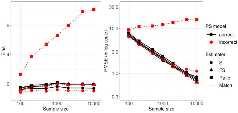
Figure 4: Bias and root mean squared error (RMSE) of the classical subclassification estimator (S), the full subclassification estimator (FS), the Ratio estimator (Ratio) and the matching estimator (Match) under Chan et al., (2016)’s setting.

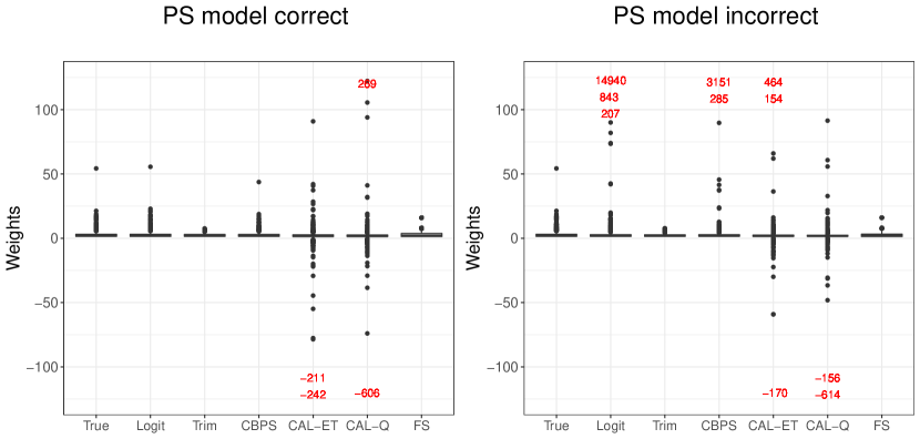
Figure 5: Distributions of weight estimates with various weighting scheme with a random simulated data set of sample size 1000. Weights outside of the plot range are annotated on the boarders.

S9 Descriptive statistics for the NHANES data

Following Chan et al., (2016), we control for the following potential confounders in our analysis: child age, child gender, child race (black, Hispanic versus others), coming from a family above 200% of the federal poverty level, participation in Special Supplemental Nutrition (SSN) Program for Women Infants and Children, participation in the Food Stamp Program, childhood food security as measured by an indicator of two or more affirmative responses to eight child-specific questions in the NHANES Food Security Questionnaire Module, any health insurance coverage, and the age and gender of the survey respondent (usually an adult in the family).

In Table 5 we provide summary statistics for potential confounders and outcome measure by participation status in the school meal programs.

Table 5: Baseline characteristics and outcome measure by participation status in the school meal programs

	Participated	Not participated
	(N=1284)	(N=1046)
Child Age, mean (SD)	10.1 (3.5)	9.9 (4.4)
Child Male, N (%)	657 (51.2%)	549 (52.5%)
Black, N (%)	396 (30.8%)	208 (19.9%)
Hispanic, N (%)	421 (32.8%)	186 (17.8%)
Above 200% of poverty level, N (%)	317 (24.7%)	692 (66.2%)
Participation in SSN program, N (%)	328 (25.5%)	115 (11.0%)
Participation in food stamp program, N (%)	566 (44.1%)	122 (11.7%)
Childhood food security, N (%)	418 (32.6%)	155 (14.8%)
Insurance Coverage, N (%)	1076 (83.8%)	927 (88.6%)
Respondent Age, mean (SD)	38.6 (10.4)	40.3 (9.7)
Respondent Male, N (%)	506 (39.4%)	526 (50.3%)
BMI, mean (SD)	20.4 (5.5)	19.8 (5.4)

References

- Abadie and Imbens, (2016) Abadie, A. and Imbens, G. W. (2016). Matching on the estimated propensity score. Econometrica, 84(2):781–807.
- Chan et al., (2016) Chan, K. C. G., Yam, S. C. P., and Zhang, Z. (2016). Globally efficient non-parametric inference of average treatment effects by empirical balancing calibration weighting. Journal of the Royal Statistical Society. Series B, Statistical methodology, 78(3):673–700.
- Gelman and Meng, (2004) Gelman, A. and Meng, X.-L. (2004). Applied Bayesian modeling and causal inference from incomplete-data perspectives. John Wiley & Sons.
- Hainmueller, (2012) Hainmueller, J. (2012). Entropy balancing for causal effects: A multivariate reweighting method to produce balanced samples in observational studies. Political Analysis, 20(1):25–46.
- Hájek, (1971) Hájek, J. (1971). Comment on an essay on the logical foundations of survey sampling by Basu, D. Foundations of Statistical Inference, 236.
- Hirano et al., (2003) Hirano, K., Imbens, G. W., and Ridder, G. (2003). Efficient estimation of average treatment effects using the estimated propensity score. Econometrica, 71(4):1161–1189.
- Horvitz and Thompson, (1952) Horvitz, D. G. and Thompson, D. J. (1952). A generalization of sampling without replacement from a finite universe. Journal of the American Statistical Association, 47(260):663–685.
- Imai and Ratkovic, (2014) Imai, K. and Ratkovic, M. (2014). Covariate balancing propensity score. Journal of the Royal Statistical Society: Series B (Statistical Methodology), 76(1):243–263.
- Imai and Van Dyk, (2004) Imai, K. and Van Dyk, D. A. (2004). Causal inference with general treatment regimes: Generalizing the propensity score. Journal of the American Statistical Association, 99(467):854–866.
- Imbens, (2000) Imbens, G. W. (2000). The role of the propensity score in estimating dose-response functions. Biometrika, 87(3):706–710.
- Imbens and Rubin, (2015) Imbens, G. W. and Rubin, D. B. (2015). Causal Inference in Statistics, Social, and Biomedical Sciences. Cambridge University Press.
- Kang and Schafer, (2007) Kang, J. D. Y. and Schafer, J. L. (2007). Demystifying double robustness: A comparison of alternative strategies for estimating a population mean from incomplete data. Statistical Science, 22(4):523–539.
- Liu et al., (2016) Liu, L., Hudgens, M. G., and Becker-Dreps, S. (2016). On inverse probability-weighted estimators in the presence of interference. Biometrika, 103(4):829–842.
- Lunceford and Davidian, (2004) Lunceford, J. K. and Davidian, M. (2004). Stratification and weighting via the propensity score in estimation of causal treatment effects: A comparative study. Statistics in Medicine, 23(19):2937–2960.
- McCaffrey et al., (2004) McCaffrey, D. F., Ridgeway, G., and Morral, A. R. (2004). Propensity score estimation with boosted regression for evaluating causal effects in observational studies. Psychological Methods, 9(4):403.
- Myers and Louis, (2007) Myers, J. A. and Louis, T. A. (2007). Optimal propensity score stratification. Johns Hopkins University, Dept. of Biostatistics Working Papers. Working Paper 155.
- Newey, (1994) Newey, W. K. (1994). Series estimation of regression functionals. Econometric Theory, 10(01):1–28.
- Newey et al., (1998) Newey, W. K., Hsieh, F., and Robins, J. (1998). Undersmoothing and bias corrected functional estimation. Working Paper, MIT.
- Paninski and Yajima, (2008) Paninski, L. and Yajima, M. (2008). Undersmoothed kernel entropy estimators. Information Theory, IEEE Transactions on, 54(9):4384–4388.
- Robins et al., (2000) Robins, J. M., Hernan, M. A., and Brumback, B. (2000). Marginal structural models and causal inference in epidemiology. Epidemiology, 11(5):550–560.
- Robins et al., (1994) Robins, J. M., Rotnitzky, A., and Zhao, L. P. (1994). Estimation of regression coefficients when some regressors are not always observed. Journal of the American Statistical Association, 89(427):846–866.
- Rosenbaum, (1987) Rosenbaum, P. R. (1987). Model-based direct adjustment. Journal of the American Statistical Association, 82(398):387–394.