On the inclusion of the diagonal Born-Oppenheimer correction in surface hopping methods

Abstract

The diagonal Born-Oppenheimer correction (DBOC) stems from the diagonal second derivative coupling term in the adiabatic representation, and it can have an arbitrary large magnitude when a gap between neighbouring Born-Oppenheimer (BO) potential energy surfaces (PESs) is closing. Nevertheless, DBOC is typically neglected in mixed quantum-classical methods of simulating nonadiabatic dynamics (e.g., fewest-switch surface hopping (FSSH) method). A straightforward addition of DBOC to BO PESs in the FSSH method, FSSH+D, has been shown to lead to numerically much inferior results for models containing conical intersections. More sophisticated variation of the DBOC inclusion, phase-space surface-hopping (PSSH) was more successful than FSSH+D but on model problems without conical intersections. This work comprehensively assesses the role of DBOC in nonadiabatic dynamics of two electronic state problems and the performance of FSSH, FSSH+D, and PSSH methods in variety of one- and two-dimensional models. Our results show that the inclusion of DBOC can enhance the accuracy of surface hopping simulations when two conditions are simultaneously satisfied: 1) nuclei have kinetic energy lower than DBOC and 2) PESs are not strongly nonadiabatically coupled. The inclusion of DBOC is detrimental in situations where its energy scale becomes very high or even diverges, because in these regions PESs are also very strongly coupled. In this case, the true quantum formalism heavily relies on an interplay between diagonal and off-diagonal nonadiabatic couplings while surface hopping approaches treat diagonal terms as PESs and off-diagonal ones stochastically.

I Introduction

The commonly used adiabatic representation defines nuclear dynamics on multiple electronic surfaces that are coupled through terms resulted from the nuclear kinetic energy operator acting on the Born-Oppenheimer (BO) electronic wavefunctions.Cederbaum (2004) Kinetic energy coupling between different BO electronic states gives rise to two effects disappearing in the BO approximation: 1) Interstate (off-diagonal) derivative couplings are responsible for transferring nuclear wavepackets between electronic surfaces. 2) Second-order diagonal derivative terms, hereon referred as diagonal Born-Oppenheimer corrections (DBOCs), modify the BO PESs.Lengsfield III and Yarkony (1986) Mathematically, DBOC is a potential-like term and thus its addition to BO PES seems very reasonable in consideration of quantum nuclear dynamics. Without DBOC, BO approximation estimates for the system total energies are not variational.Brattsev (1965); Epstein (1966) In regions of close proximity of BO PESs, DBOCs can become arbitrarily large, and a nuclear wavepacket travelling on modified PESs (such surfaces are usually called adiabatic surfaces) can undergo very different dynamics compared to that on BO PESs.Ryabinkin, Joubert-Doriol, and Izmaylov (2014) Generally, in nonadiabatic regions for adequate modelling of true quantum nuclear dynamics in the adiabatic representation, all terms related to potential and kinetic energies as well as geometric phase appearing in conical intersections must be taken into account.Ryabinkin, Joubert-Doriol, and Izmaylov (2014)

Often to address nonadiabatic dynamics in large systems mixed quantum-classical (MQC) methods such as FSSH and Ehrenfest are adequate and computationally feasible.Tully (1990, 1998) Nuclear dynamics in these methods is simplified to the classical level and is governed by forces obtained from variously defined electronic surfaces. A natural question in this context is whether adding DBOC to electronic surfaces can improve the performance of these methods? A nontrivial character of this question is related to the fact that in MQC methods we do not have quantum nuclear wavepackets. Thus, although DBOC is necessary for the correct dynamics of nuclear wavepackets, it may not necessarily improve dynamics of classical particles. Indeed, for conical intersection problems, a straightforward addition of DBOC to BO PESs in the FSSH method was found to be detrimental for dynamics.Gherib, Ryabinkin, and Izmaylov (2015) In further discussion we will refer to this modification of FSSH as FSSH+D. Moreover, in the Ehrenfest method, DBOC inclusion breaks down the invariance of the approach with respect to the adiabatic-to-diabatic electronic basis transformation. One of the reasons why DBOC is detrimental in CI problems is the absence of explicit account of the geometric phase in MQC methods.Gherib, Ryabinkin, and Izmaylov (2015) However, not all problems have CIs that affect nonadiabatic dynamics, therefore including DBOC in surface hopping approaches for non-CI problems may have its benefits and has been advocated in Ref. Akimov and Prezhdo, 2013; Shenvi, 2009.

Recently, Shenvi proposed an alternative to FSSH, the phase-space surface-hopping (PSSH) method.Shenvi (2009) The key idea behind PSSH is the use of phase-space surfaces that incorporate both DBOC and first derivative couplings. It was deemed that such surfaces would be coupled weaker than corresponding BO PESs in FSSH. On a few one-dimensional model systems it was shown that PSSH performs very well and generally better than FSSH+D. Surprisingly, no comparison of PSSH results with those of the original FSSH method has been done. Also, the PSSH method have not been tried in situations when DBOC is very large or diverging (e.g., conical intersections).

In this work we would like to assess whether including DBOC can improve results of nonadiabatic dynamics in FSSH+D and PSSH methods based on results in few representative one- and two-dimensional models. If there are such cases which method among these two should be preferred. The rest of the paper is organized as follows. Section II A reviews the fully quantum formalism that gives rise to DBOC. Section II B illustrates how FSSH, FSSH+D, and PSSH classical equations of motion (EOM) can be rationalized within a general framework. In Section III, nonadiabatic numerical simulations of various 1D and 2D models are presented and show the strengths and limitations of FSSH, FSSH+D and PSSH. Section IV concludes the work by summarizing main results and discussing potential future challenges. Atomic units will be used throughout this work.

II Theory

II.1 Diagonal Born-Oppenheimer correction

To see how DBOC emerges in the exact quantum-mechanical formalism let us start with the exact quantum mechanical molecular Hamiltonian

$$\hat{H}_{m}=\hat{T}_{n}+\hat{H}_{e},$$ (1)

where $\hat{T}_{n}$ is the kinetic nuclear energy operator and $\hat{H}_{e}$ is the electronic Hamiltonian, the sum of the total molecular potential energy and the kinetic electronic energy. The adiabatic representation involves the basis of electronic functions $\{\ket{\phi_{j}(\textbf{R})}\}$ that solve the electronic time-independent Schrödinger equation (TISE) for a fixed nuclear configuration R

$$\hat{H}_{e}\ket{\phi_{i}(\textbf{R})}=E_{i}(\textbf{R})\ket{\phi_{i}(\textbf{R})}.$$ (2)

Using $\{\ket{\phi_{j}(\textbf{R})}\}$, an eigenfunction of $\hat{H}_{m}$ can be written as

$$\Psi(\textbf{r},\textbf{R})=\sum_{j}\phi_{j}(\textbf{r};\textbf{R})\chi_{j}(\textbf{R}),$$ (3)

where nuclear counterparts $\chi_{j}(\textbf{R})$ can be obtained from projecting the full TISE, $\hat{H}_{m}\Psi(\textbf{r},\textbf{R})=\mathcal{E}\Psi(\textbf{r},\textbf{R})$, onto the electronic basis

$$\sum_{j}\left[\braket{\phi_{i}(\textbf{R})}{\hat{T}_{n}}{\phi_{j}(\textbf{R})}+\delta_{ij}E_{j}\right]\chi_{j}(\textbf{R})=\mathcal{E}\chi_{i}(\textbf{R}).$$ (4)

For the sake of simplicity we will only consider one nuclear degree of freedom (DOF) with a nuclear mass $M$

$$\hat{T}_{n}=-\frac{1}{2M}{\nabla_{\textbf{R}}}^{2},$$ (5)

the following consideration can be straightforwardly extended to more nuclear DOF. Due to the parametric dependency of adiabatic states on R, the evaluation of $\braket{\phi_{i}(\textbf{R})}{\hat{T}_{n}}{\phi_{j}(\textbf{R})}$ in Eq. (4) requires use of the chain rule in the action of the Laplacian on $\ket{\phi_{j}(\textbf{R})}$

$$\braket{\phi_{i}(\textbf{R})}{\hat{T}_{n}}{\phi_{j}(\textbf{R})}=-\frac{1}{2M}[\delta_{ij}{\nabla_{\textbf{R}}}^{2}$$ (6)

$$+2\braket{\phi_{i}(\textbf{R})}{\nabla_{\textbf{R}}\phi_{j}(\textbf{R})}\nabla_{\textbf{R}}+\braket{\phi_{i}(\textbf{R})}{{\nabla_{\textbf{R}}}^{2}\phi_{j}(\textbf{R})}].$$

By introducing a resolution of the identity $\sum_{k}\ket{\phi_{K}(\textbf{R})}\bra{\phi_{K}(\textbf{R})}$ inside the last component in Eq. (II.1), the matrix elements of the nuclear kinetic energy can be expressed as

$$\braket{\phi_{i}(\textbf{R})}{\hat{T}_{n}}{\phi_{j}(\textbf{R})}=-\frac{1}{2M}[\delta_{ij}{\nabla_{\textbf{R}}}^{2}$$

$$+\braket{\phi_{i}(\textbf{R})}{\nabla_{\textbf{R}}\phi_{j}(\textbf{R})}\nabla_{\textbf{R}}+\nabla_{\textbf{R}}\braket{\phi_{i}(\textbf{R})}{\nabla_{\textbf{R}}\phi_{j}(\textbf{R})}$$

$$+\sum_{k}\braket{\phi_{i}(\textbf{R})}{\nabla_{\mathbf{R}}\phi_{k}(\textbf{R})}\braket{\phi_{k}(\textbf{R})}{\nabla_{\mathbf{R}}\phi_{j}(\textbf{R})}].$$ (7)

For a system with two electronic states, kinetic energy matrix operator, $\mathbf{T_{n}}$, takes the following form

$$\mathbf{T_{n}}=-\frac{1}{2M}\begin{pmatrix}{\nabla_{\textbf{R}}}^{2}-{\mathbf{d}_{12}}^{2}&\nabla_{\mathbf{R}}\cdot\mathbf{d}_{12}+\mathbf{d}_{12}\cdot\nabla_{\mathbf{R}}\\ \nabla_{\mathbf{R}}\cdot\mathbf{d}_{21}+\mathbf{d}_{21}\cdot\nabla_{\mathbf{R}}&{\nabla_{\textbf{R}}}^{2}-{\mathbf{d}_{21}}^{2}\end{pmatrix}.$$ (8)

The components $\mathbf{d}_{12}=\braket{\phi_{1}(\textbf{R})}{\nabla_{\mathbf{R}}\phi_{2}(\textbf{R})}$ and ${\mathbf{d}_{12}}^{2}/(2M)$ are the nonadiabatic coupling vector (NAC) and DBOC, respectively. DBOC is a function of R and a diagonal element of the total molecular Hamiltonian projected in the electronic adiabatic basis

$$\textbf{H}_{m}=\mathbf{T_{n}}+\begin{pmatrix}E_{1}(\textbf{R})&0\\ 0&E_{2}(\textbf{R})\end{pmatrix}.$$ (9)

Thus, DBOC can be summed to the BO PESs and regarded as a second-order correction in $\hbar$

$$\tilde{E_{j}}(\textbf{R})=E_{j}(\textbf{R})+\frac{{\mathbf{d}_{12}}^{2}}{2M}.$$ (10)

We will refer to $\tilde{E_{j}}(\textbf{R})$ surfaces as adiabatic PESs in contrast with $E_{j}(\textbf{R})$ which are referred to as BO PESs. Adiabatic PESs, $\tilde{E_{j}}$, have always a larger value than corresponding BO PESs, $E_{j}(\textbf{R})$. The difference between two types of PESs grows with the length of NAC which is inversely proportional to the difference between electronic energies

$$\mathbf{d}_{12}=\frac{\braket{\phi_{1}(\textbf{R})}{\nabla_{\textbf{R}}H}{\phi_{2}(\textbf{R})}}{E_{2}-E_{1}},$$ (11)

and hence, both NAC and DBOC become large in the region of close proximity of two BO PESs.

II.2 Surface hopping methods

Here, we provide a uniform framework rationalizing various versions of classical nuclear EOM used in surface hopping methods.

FSSH:

Let us transform the molecular Hamiltonian, $\hat{H}_{m}$ in Eq. (1) to its classical analogue $H_{m}^{\textrm{cl}}$, by converting $\hat{T}_{n}$ to ${{\textbf{P}}^{2}}/{(2M)}$, where P is the classical nuclear momentum. This step amounts to substituting the quantum operator $-i\nabla_{\textbf{R}}$ by the P variable. The resulting molecular Hamiltonian is

$$\hat{H}_{m}^{\textrm{cl}}=\frac{{\textbf{P}}^{2}}{2M}+\hat{H}_{e}.$$ (12)

By projecting $\hat{H}_{m}^{\textrm{cl}}$ onto the adiabatic basis we obtain

$$\hat{H}_{m}^{\textrm{cl}}=\delta_{ij}\left(\frac{{\textbf{P}}^{2}}{2M}+E_{i}(\textbf{R})\right),$$ (13)

which corresponds to uncoupled EOM whereby nuclei are classical and evolve on BO PESs $E_{i}(\textbf{R})$.

It should be noted that by following this route, DBOC does not emerge due to the quantum-classical transformation that removes quantum kinetic energy operator before the adiabatic electronic basis is introduced.

FSSH+D:

An alternative route to the classical nuclear EOM involves inverting the order of the quantum-classical transformation and the projection to the adiabatic electronic basis. This inversion amounts to starting from Eq. (9) instead of Eq. (1) and leads to the Hamiltonian

$$H_{n}^{1)\rightarrow 2)}=\begin{pmatrix}\frac{\textbf{P}^{2}}{2M}+\tilde{E}_{1}(\textbf{R})&-\frac{i\mathbf{d}_{12}\cdot{\textbf{P}}}{M}\\ \frac{i\mathbf{d}_{12}\cdot{\textbf{P}}}{M}&\frac{\textbf{P}^{2}}{2M}+\tilde{E}_{2}(\textbf{R})\end{pmatrix}.$$ (14)

From thereon, we can remove the off-diagonal terms and obtain uncoupled classical Hamiltonians corresponding to two electronic states. In this alternative route, the potential on which the nuclei are evolving are DBOC-modified potentials $\tilde{E}_{i}(\textbf{R})$.

PSSH:

If one does not discard the off-diagonal couplings in the Hamiltonian $H_{n}^{1)\rightarrow 2)}$ but rather diagonalizes $H_{n}^{1)\rightarrow 2)}$ to obtain an electronic basis parametrically dependent on R and P

$$H_{n}^{1)\rightarrow 2)}\ket{n_{i}^{\rm PS}(\textbf{R},\textbf{P})}=E_{i}^{\rm PS}\ket{n_{i}^{\rm PS}(\textbf{R},\textbf{P})},$$ (15)

$\{\ket{n_{i}^{\rm PS}(\textbf{R},\textbf{P})}\}$ is referred as phase-space adiabatic representation. $E_{i}^{\rm PS}$ are phase-space total energies and for a two-level system they are

$$E_{\pm}^{\rm PS}(\textbf{R},\textbf{P})= \frac{\textbf{P}^{2}}{2M}+\frac{1}{2}\left(\tilde{E}_{1}(\textbf{R})+\tilde{E}_{2}(\textbf{R})\right)$$

$$\pm\frac{1}{2}\sqrt{\left({E}_{1}(\textbf{R})-{E}_{2}(\textbf{R})\right)^{2}+4\left(\frac{\mathbf{d}_{12}\cdot{\textbf{P}}}{M}\right)^{2}}.$$ (16)

For the excited state, DBOC is enhanced by the NAC related term while for the ground state DBOC can be compensated by the NAC term. Hence, the phase-space representation can lift the degeneracy in the adiabatic representation. Far from strongly coupled regions, phase-space and adiabatic representation electronic wavefunctions and PESs converge to each other. The classical trajectories for nuclei on a single phase-space surface $E_{\pm}^{\rm PS}$ can be obtained using Hamilton’s EOM

$$\dot{\textbf{R}}_{\pm}=\frac{\partial E_{\pm}^{\rm PS}}{\partial\textbf{P}},\quad\dot{\textbf{P}}_{\pm}=-\frac{\partial E_{\pm}^{\rm PS}}{\partial\textbf{R}}.$$ (17)

In all these approaches nuclear dynamics experience stochastic hops between PESs, the hopping probabilities are proportional to NACs and their explicit expressions and further details on the electronic dynamics can be found in the supplementary material.mis

III Numerical simulations

To determine whether DBOC could be beneficial in surface hopping approaches and to assess more extensively the accuracy of PSSH and FSSH+D, we consider in this section three types of systems: 1) two flat one-dimensional BO PES coupled nonadiabatically, 2) one-dimensional avoided crossing model with different diabatic couplings, 3) two-dimensional linear vibronic coupling (2D-LVC) models containing CIs in the adiabatic representation. All FSSH and FSSH+D simulations were performed in the adiabatic representation.

III.1 Flat BO PESs

We begin by considering model 2 of the PSSH original paperShenvi (2009) (Fig. 1). The molecular Hamiltonian in the diabatic representation for this model is

$$H^{\rm D}_{\rm F}=-\frac{1}{2M}\frac{\partial^{2}}{\partial{R}^{2}}\cdot\mathbf{1}_{2}+\begin{bmatrix}-A\cos(\theta)&A\sin(\theta)\\ A\sin(\theta)&A\cos(\theta)\end{bmatrix},$$ (18)

where $\theta=C\pi\left(\tanh(D{R})+1)\right)$, $A=0.005$, $C=5.5$, $D=0.8$ and $M=2000$ a.u. The model involves two flat BO PES coupled with NAC that has a $\mathrm{sech}\,^{2}({R})$ form.

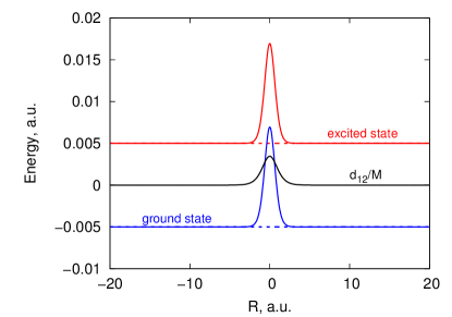
Figure 1: Nonadiabatic coupling (solid black) and PESs for the model with flat BO PESs: ground (dashed blue) and excited (dashed red) BO PESs, ground (solid blue) and excited (solid red) adiabatic PESs.

The exact quantum dynamics simulations were performed using the split operator method on a grid of 2048 points inside a box of length 40 a.u. and a time-step of 0.1 fs. The initial wavepacket was a Gaussian $\Psi({R},0)=e^{i\braket{{P}}{R}}e^{-\left(({R}-\braket{R})/\sigma\right)^{2}}$ with a width parameter $\sigma=20/\braket{{P}}$. The SH simulations were done with 2000 trajectories for all three SH methods, and time-steps of 0.025 fs, 0.025 fs, and 0.01 fs for FSSH, PSSH, and FSSH+D, respectivley. The initial distribution of positions and momenta for the SH simulations was taken as the Wigner transform of $\Psi({R},0)$.

The initial assessment in Ref. Shenvi, 2009 investigated the ability of FSSH+D and PSSH to simulate transmission of a nuclear wavepacket starting from $\braket{{R}}=-10$. It was shown that in the case of low initial $\braket{{P}}$, PSSH can model transmission more accurately that FSSH+D (Fig. 2). To determine whether the failure of FSSH+D simulations resides in the presence of DBOC, we have redone the nonadiabatic dynamics using FSSH. As can be seen from Fig. 2, FSSH can in fact model transmission in this model for most cases (FSSH deviates when $\braket{{P}}\in(6,7)$). In this model DBOC acts as a barrier that reflects particles with low momenta. DBOC elimination removes the reflection and allows particles to pass through even at low momenta. Thus, in this particular model, DBOC should not be simply added to BO PESs.

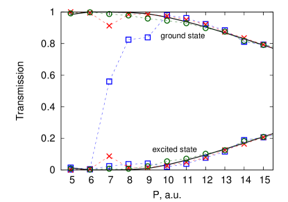
Figure 2: Probability of transmission on the ground and excited states with respect to the initial average momentum of the distribution located on the ground state: exact quantum (black lines), FSSH (red crosses), FSSH+D (blue squares), and PSSH (green circles). The dashed lines are not representing results between the points but serve as an eye guide.

The deviation of FSSH for $\braket{{P}}\in(6,7)$ can be explained by considering that the lowest momentum that permits hopping is ${P}_{\rm min}=\sqrt{2M\Delta E_{12}}\approx 6.3$ a.u. Thus, when a classical particle has ${P}\approx{P}_{\rm min}$, upon hopping to the excited state it will have a momentum close to zero. Because the BO PESs are flat, there is no source of acceleration and hopped particles remain frozen on the excited state.

In this model, the difference between curvatures of the potential energy surfaces in FSSH+D and PSSH methods stems from the square root term in Eq. (II.2). This term partially cancels the repulsive barrier coming from DBOC for the ground state in PSSH (see Fig. 3). Thus the ground state DBOC repulsive barrier is effectively lower in PSSH than in FSSH+D. This allows PSSH to have good transmission for PSSH even at low momenta (Fig. 2).

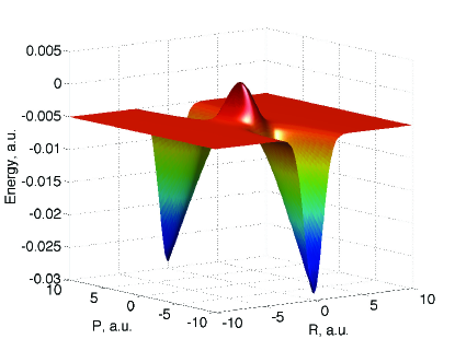
Figure 3: Phase-space ground state potential energy surface without the kinetic energy like term, ${E}_{-}^{\rm PS}-{P}^{2}/(2M)$, for the model with flat BO PESs.

Following this logic of compensation there should be a point in the ${P}$-space where the momentum is so low, that DBOC cannot be compensated by the square root term. To determine how well PSSH describes the transition from transmitting to reflecting regimes, simulations for the transmission coefficient have been performed for low momenta (see Fig. 4). The transmission coefficients show that for low momenta, DBOC completely repulses classical particles in FSSH+D, while in FSSH all particles can pass through the nonadiabatic region. The exact dynamics shows that in the considered range of momenta, the nuclear wavepacket bifurcates on a single surface while crossing the nonadiabatic region. PSSH captures this phenomenon accurately by quantifying adequately the fraction of the distribution that is transmitted. Note that at this range of momenta, the nuclear subsystem in all surface hopping variations does not have enough kinetic energy to hop, therefore, the dynamics is purely adiabatic.

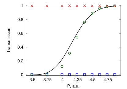
Figure 4: Probability of transmission on the ground state with respect to the initial average momentum of the distribution located on the ground state: exact quantum (black line), FSSH (red crosses), FSSH+D (blue squares), and PSSH (green circles)

It has been noted in Ref. Shenvi, 2009 that momenta of classical particles in PSSH increase while crossing the nonadiabatic region. However, this does not imply an increase in velocity. Indeed as shown in Fig. 5, particles in PSSH actually slow down while crossing the nonadiabatic region on the ground state. In PSSH, this slow down comes from the square root term in the potential energy, which has a negative contribution on the ground state phase-space PES. In the exact quantum dynamics, the slow-down occurs due to the partial transfer of the wavepacket population to the excited state. A consequent increase in potential energy leads to a decrease in the kinetic nuclear energy. In SH methods, the initial average momentum $\braket{{P}}=5$ a.u. does not allow hops to occur. In FSSH, the nuclear coordinate does not experience any force and evolves similarly to the centre of the nuclear wavepacket on a flat PES in the quantum BO dynamics. Due to DBOC, FSSH+D overestimates a repulsive character of the electronic potential. Therefore both FSSH and FSSH+D fail to model accurately the spatial evolution of the nuclear coordinate when nonadiabatic couplings are non-negligible. Only PSSH models accurately the slow-down that a nuclear wavepacket experiences in the true quantum dynamics in a nonadiabatic region.

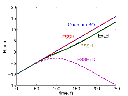
Figure 5: The average position of the nuclear distribution in different methods as a function of time: SH variants (dashed lines) and quantum calculations (full lines).

In the excited phase-space PES, the square root term adds on to DBOC and increases the potential energy barrier classical particles need to surmount in order to pass through nonadiabatic region (Fig. 6). By performing the same simulations as Fig. 2, but starting from the excited adiabatic state, the nuclear wavepacket is repulsed at higher momenta (see Fig. 7). Here, FSSH fails completely in the region of low momenta by showing almost complete transmission. Both FSSH+D and PSSH reproduce quantum dynamics very well.

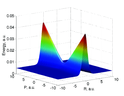
Figure 6: Phase-space excited state potential energy surface without the kinetic energy like term, ${E}_{-}^{\rm PS}-{P}^{2}/(2M)$, for the model with flat BO PESs.

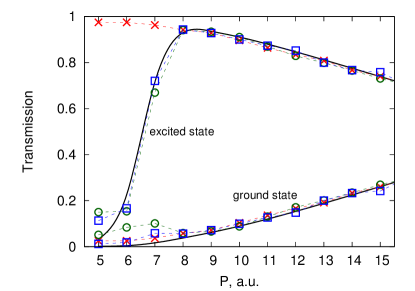
Figure 7: Probability of transmission on the ground and excited states with respect to the initial average momentum of the distribution located on the excited state: exact quantum (black lines), FSSH (red crosses), FSSH+D (blue squares), and PSSH (green circles). The dashed lines are not representing results between the points but serve as an eye guide.

III.2 Avoided crossing

While the previous model successfully showed regimes where FSSH, FSSH+D and PSSH differ, it does not describe situations where BO PESs come very close to each other. An avoided crossing model allows to explore such regimes, its diabatic Hamiltonian is

$$H^{\rm D}_{\rm AC}=-\frac{1}{2M}\frac{\partial^{2}}{\partial{R}^{2}}\mathbf{1}_{2}+\begin{bmatrix}-b{R}&c\\ c&b{R}\end{bmatrix},$$ (19)

where $b=0.01$ is fixed and $c$ will be varied. In the adiabatic representation, this model has BO PESs whose lowest energy gap is $\Delta E_{12}=2c$ and DBOC is

$$\frac{d_{12}^{2}}{2M}=\frac{b^{2}c^{2}}{8M(c^{2}+b^{2}R^{2})^{2}}$$ (20)

(see Fig. 8). The initial nuclear wavepacket was $\Psi({R},0)=e^{-4\left({R}-5\right)^{2}}$. The nuclear mass, $M$, the number of trajectories, and time-step lengths were taken as in the model with flat BO PESs.

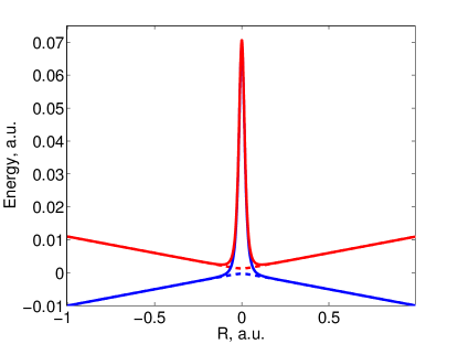
Figure 8: BO (dashed) and adiabatic (solid) PESs of the avoided crossing model with $c=3\times 10^{-4}$.

The property of interest is the probability for the nuclear wavepacket starting from the excited state to transfer to the ground state. When the diabatic coupling constant, $c$, is high, the wavepacket is expected to remain on the upper adiabatic state for the entire simulation while for low diabatic constant, a nearly complete transfer to the lower adiabatic state is envisioned. Figure 9 presents results for a range of $c$’s that corresponds to a range of DBOC maximum energies of $6.3\times 10^{-3}$ – $6.3\times 10^{-5}$ a.u. These energies are much smaller than the kinetic energy that the wave-packet gains at $R=0$, $5\times 10^{-2}$ a.u., and thus, all SH variations model nuclear dynamics accurately (Fig. 9).

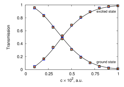
Figure 9: Probability of transmission on the ground state with respect to the diabatic coupling constant, $c$: exact quantum (black line), FSSH (red crosses), FSSH+D (blue squares), and PSSH (green circles). The initial nuclear distribution is on the excited state.

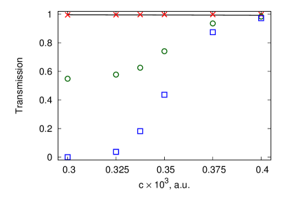
Figure 10: Probability of transmission on the ground and excited states with respect to diabatic coupling constant, $c$: exact quantum (black lines), FSSH (red crosses), FSSH+D (blue squares), and PSSH (green circles). The initial nuclear distribution is on the excited state.

Decreasing $c$ to values where DBOC maxima are comparable or higher than the kinetic energy of the nuclear wave-packet at $R=0$ separates all SH methods, see Fig. 10. In both FSSH+D and PSSH, the system transfer to the ground state is significantly inhibited by increasing DBOC. Qualitatively, for both methods the reason for this deviation is similar but it is easier to illustrate it in the FSSH+D case (see Fig. 11). In FSSH+D, a repulsive DBOC potential reduces nuclear momentum of a particle and as a consequence the nonadiabatic transfer probability to zero before the particle reaches the intersection $R=0$. This allows the nonadiabatic transfer to take place only before the intersection where the particle will not have enough kinetic energy to overcome the DBOC induced barrier on the ground state.

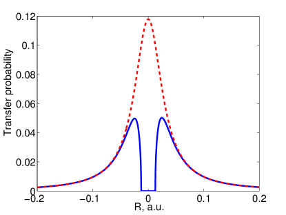
Figure 11: Transfer probability ($d_{12}P/M$) as a function of position for the avoided crossing model with $c=3\times 10^{-4}$: FSSH (red dashed) and FSSH+D (solid blue). $P$ as a function of $R$ is evaluated using $\sqrt{2M\max(E_{0}-E_{+}(R),0)}$, where $E_{0}=-bR_{0}$ is the initial energy with $R_{0}=-5$ a.u. and $E_{+}(R)$ are excited state PESs with and without DBOC.

PSSH suffers less from the DBOC inclusion (Fig. 10) because of two reasons: First, if the non-adiabatic transfer happens to the ground state, DBOC can be compensated there by the $d_{12}P/M$ term. Second, PSSH particles have generally larger velocities on the excited state in the nonadiabatic region. In this region the difference between BO PES becomes negligible ($E_{2}(R)-E_{1}(R)\approx 0$) and the nuclear velocity in PSSH can be approximated as

$$\dot{R}_{\pm}=\frac{P}{M}\left(1\pm\left|\frac{d_{12}}{P}\right|\right).$$ (21)

Thus, nuclear DOF can experience an acceleration if they are on the phase-space excited state and a deceleration if they are on the phase-space ground state. For classical particles the DBOC effect will reduce $P$. However, due to $d_{12}$ the $P$ reduction does not lead to velocity reduction. In other words, in PSSH, nuclei can use $d_{12}$ to overcome a part of the DBOC repulsion.

On the other hand FSSH correlates with the exact dynamics and shows complete transfer. In the absence of DBOC, nothing prevents classical particles in FSSH from accessing the region of strong nonadiabatic coupling and hopping to the ground state (Fig. 11). The final outcome will not depend on whether a hop taken place before or after the intersection because the ground state does not have a DBOC induced barrier. Thus for weakly diabatically coupled avoided crossing models, FSSH surpasses both PSSH and FSSH+D in describing excited state dynamics.

Interestingly, in the small $c$ case, interpreting DBOC as a repulsive potential in quantum dynamics is incorrect because in the nonadiabatic region ($R\approx 0$) NAC becomes very large

$$d_{12}=\frac{bc}{2(c^{2}+b^{2}R^{2})}\rightarrow\frac{b}{2c},\quad R\rightarrow 0$$ (22)

and thus the adiabatic surface interpretation of the dynamics is misleading. Instead, the simplest quantum dynamical picture emerges in the diabatic representation where for very small $c$’s dynamics is almost fully confined to a single diabatic surface. In the diabatic representation, DBOC does not appear and the absence of any other repulsive potentials on the diabats illustrates that there is a complete cancellation of diagonal and off-diagonal derivative coupling terms when one goes from the adiabatic representation to the diabatic one. Moreover, if one subtracts DBOC from the adiabatic nuclear Hamiltonian [Eq. (9)] the transfer dynamics becomes slower and less efficient. Thus, effectively, removing DBOC introduces the repulsive potential in the quantum dynamics. To understand this, it is instructive to transform the adiabatic Hamiltonian without DBOC to the diabatic representation where subtracting the DBOC leads to two dips on the diabats at the point of their intersections (Fig. 12). These dips give rise to the over-barrier reflection of the wave-packet traveling on a diabat and thus reduces the efficiency of passing the crossing point (Fig. 13). This is purely quantum effect and it will be lost when classical mechanics is used on the same potential.

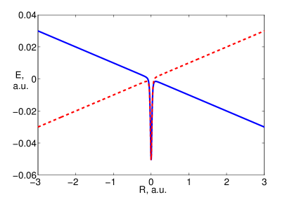
Figure 12: Diabatic surfaces (solid blue and dashed red) for the avoided crossing model when DBOC is subtracted from the Hamiltonian in the adiabatic representation, $c=3.5\times 10^{-4}$.

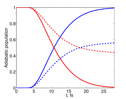
Figure 13: Dynamics of the adiabatic population starting from the initial wavepacket on the excited state, $M=200$ a.u., $c=3.5\times 10^{-4}$: red and blue are populations of the excited and ground states, solid and dashed are with and without DBOC, respectively.

III.3 Conical intersections

Conical intersections are ubiquitous in molecular systems and allow for ultra-fast transfer between electronic states. At the exact point of intersection, electronic states are degenerate and give rise to an infinitely large DBOC, which have been shown to decrease the rate of electronic transitions in FSSH+D.Gherib, Ryabinkin, and Izmaylov (2015) Analysis of the interplay between DBOC and other nonadiabatic terms in fully quantum dynamics for CIs is complicated by appearance of a nontrivial geometric phase and is provided in Ref. Ryabinkin, Joubert-Doriol, and Izmaylov, 2014. It was found that for CIs, DBOC is only compensated by other terms when the geometric phase is included. Without geometric phase, DBOC creates repulsive potential for the quantum nuclear wavepacket, therefore, since SH methods do not have geometric phase for the nuclear wave-function, they also experience DBOC as a repulsive potential even in a greater extent because classical particles cannot tunnel under DBOC.

To determine whether PSSH can model population dynamics through CIs, we consider the 2D-LVC model

$$H^{\rm D}_{\rm LVC}=T_{2D}\mathbf{1}_{2}+\begin{bmatrix}V_{11}&V_{12}\\ V_{12}&V_{22}\end{bmatrix},$$ (23)

where

$$V_{11} =\frac{1}{2}\left[\omega_{1}^{2}\left(x+\frac{a}{2}\right)^{2}+\omega_{2}^{2}y^{2}+{\Delta}\right],$$ (24)

$$V_{22} =\frac{1}{2}\left[\omega_{1}^{2}\left(x-\frac{a}{2}\right)^{2}+\omega_{2}^{2}y^{2}-{\Delta}\right],$$ (25)

$$V_{12} =cy.$$ (26)

This diabatic model corresponds to two paraboloids shifted in space in the $x$-direction by $a$ and in energy by $\Delta$. Three molecular systems whose ultrafast excited state dynamics is well represented with 2D-LVC have been investigated: bis(methylene) adamantyl cation (BMA),Blancafort, Hunt, and Robb (2005) butatriene cationKöppel, Domcke, and Cederbaum (1984); Cederbaum et al. (1977); Cattarius et al. (2001); Sardar et al. (2008); Burghardt, Gindensperger, and Cederbaum (2006); Gindensperger, Burghardt, and Cederbaum (2006) and pyrazine.Seidner, Domcke, and von Niessen (1993); Woywod et al. (1994); Sukharev and Seideman (2005) Their 2D-LVC parameters are given in Table 1.

Table 1: Parameters of the 2D-LVC Hamiltonian, Eq. (23) for the three CI systems.

$\omega_{1}$	$\omega_{2}$	$a$	$c$	$\Delta$
Bis(methylene) adamantyl cation
$7.743\times 10^{-3}$	$6.680\times 10^{-3}$	31.05	$8.092\times 10^{-5}$	0.000
Butatriene cation
$9.557\times 10^{-3}$	$3.3515\times 10^{-3}$	20.07	$6.127\times 10^{-4}$	0.020
Pyrazine
$3.650\times 10^{-3}$	$4.186\times 10^{-3}$	48.45	$4.946\times 10^{-4}$	0.028

MQC simulations are done using 2000 trajectories and 0.05, 0.01, and 0.001 fs time-steps for FSSH, FSSH+D, and PSSH, respectively. Similarly to FSSH, in PSSH each trajectory carries both an electronic wavefunction and an active electronic surface. However, in PSSH these quantities correspond to the phase-space basis and PESs, which are identical to their adiabatic counterparts far from the nonadiabatic region, but differ from them when adiabatic states become coupled. To model adiabatic population dynamics using PSSH, one is faced with the following problem: How to use phase-space information to calculate the adiabatic populations ?

A straightforward procedure consists in rotating the electronic wavefunction to the adiabatic representation using a unitary matrix and taking absolute squares of the complex amplitudes to obtain the adiabatic populations. An alternative method consists in ignoring the electronic wavefunction and decomposing the active phase-space surface into adiabatic state weights. Both methods were used in the following simulations, and we will denote population calculations based on the amplitudes of electronic wavefunctions as PSSH-A and based on the active phase-space surface as PSSH-S.

For all CI models, PSSH nonadiabatic dynamics is in a worse agreement with the exact one than that of FSSH (see Figs. 14-16). However, PSSH clearly outperforms FSSH+D. In the cases of BMA (Fig. 14) and pyrazine (Fig. 16), there is only partial population transfer within the considered time span. This failure of PSSH does not stem from the procedure used to convert phase-space electronic information into adiabatic populations, but rather from the presence of DBOC in phase-space PESs. DBOC repulses classical particles away from regions where hops are probable.

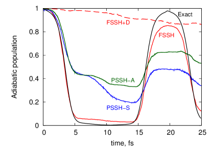
Figure 14: Excited state adiabatic population dynamics for BMA cation in different methods.

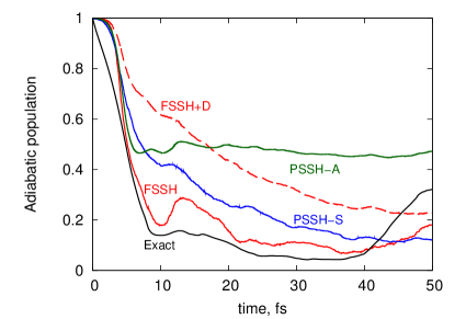
Figure 15: Excited state adiabatic population dynamics for butatriene cation in different methods.

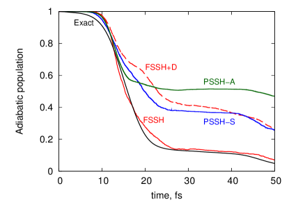
Figure 16: Excited state adiabatic population dynamics for pyrazine in different methods.

In light of the results of Fig. 10, the failure of PSSH is justified. In system with CIs, most classical particles never go through the CI, instead, the majority evolve on PESs that resemble avoided crossings. Particles travelling in regions of low diabatic couplings will experience greater DBOC and will be pushed away from nonadiabatic regions.

IV Conclusions

We systematically assessed the inclusion of DBOC in surface hopping methods for various one- and two-dimensional nonadiabatic models. It was found that for DBOC to affect dynamics its energy scale must be larger or comparable with that of the nuclear kinetic energy. In cases when DBOC is large the off-diagonal NACs are also significant. This relation makes improving BO PESs by adding DBOC to them less appealing because a PES picture is only adequate when corresponding couplings are small. Inherently, all surface hopping methods use classical mechanics to describe the nuclear motion within a PES and stochastic treatment of inter-surface couplings. Therefore the best representation for these methods needs to have low overall couplings between PESs.

When DBOC is simply added to BO PESs, the FSSH+D approach, it always brings a repulsive potential that slows down classical particles and thus makes nonadiabatic transitions less probable. For the dynamics on the excited state of the one-dimensional model with flat BO PESs this behaviour is in accord with the exact quantum nuclear dynamics. However, for the ground state dynamics of the same system and excited state dynamics of the avoided crossing and conical intersection models FSSH+D overestimates the effect of the DBOC repulsion and deviates qualitatively from the exact dynamics.

More advanced treatment of DBOC via the PSSH approach operates with phase-space PESs that account for some interplay between DBOC and off-diagonal NACs. For all cases, PSSH performed better than FSSH+D, this can be related to the DBOC compensation by NACs for the ground state dynamics and NACs contribution to velocity enhancements in nonadiabatic regions that allows particle to advance further on the excited state in spite of the DBOC repulsion. However, in very weakly coupled avoided crossing and conical intersection problems, PSSH performance was worse than the that of the original FSSH method without DBOC. We attribute this to difficulty of capturing the correct interplay between DBOC and NACs at a very localized nonadiabatic regions appearing in these problems. The full quantum formalism is capable of treating this interplay mainly because it involves quantum nuclear wavefunctions. Also, modelling a very weakly diabatically coupled avoided crossing system revealed that a repulsive potential consideration of DBOC that appears in surface hopping treatment is qualitatively incorrect. In this case DBOC is responsible for providing smooth diabatic surfaces, and its removal leads to diabatic surfaces with a prominent over-barrier reflection for a quantum nuclear wavepacket.

Applying PSSH on large molecular systems in conjunction with electronic structure methods poses a future challenge. The algorithm requires not only computing first and second-order nonadiabatic couplings but also their gradients with respect to nuclear coordinates. The latter are necessary to compute the forces acting on nuclei evolving on phase-space PESs. Furthermore, for weakly diabatically coupled avoided crossing and conical intersection problems, there is no advantage in using PSSH instead of FSSH. The former class of systems frequently appear in simulations of long range charge and energy transfers and have been referred in literature as trivial unavoided crossings.Meek and Levine (2014); Wang and Prezhdo (2014) Thus, considering relatively small range of systems where adding DBOC could improve current surface hopping approaches and additional computational expenses for DBOC evaluation it is not advisable to incorporate this quantity in the mixed quantum-classical calculations.

Current findings are also in accord with our recent work on the quantum classical Liouville equation (QCLE)Ryabinkin et al. (2014) which is a more advanced and rigorously derivable mixed quantum-classical approach.Kapral (2006) Two main steps in the QCLE derivation are a projection to adiabatic electronic states and a Wigner transformation of nuclear coordinates. These two steps do not commute and their different orders give rise to two different methods: Adiabatic-then-Wigner (AW)Ando (2002); Horenko et al. (2002) and Wigner-then-Adiabatic (WA)Kelly and Kapral (2010) QCLEs. Although two methods perform in many instances similarly,Ando and Santer (2003) based on analysis of conical intersection models and associated geometric phase effects it was found that only WA-QCLE is mathematically well defined approach.Ryabinkin et al. (2014) Interestingly, DBOC does not appear in WA-QCLE, but it is a part of AW-QCLE. Recently, FSSH approach has been connected to WA-QCLE methodSubotnik, Ouyang, and Landry (2013); Kap and in light of this connection it is natural that FSSH should not include DBOC.

V Acknowledgements

A.F.I. would like to thank Neil Shenvi for helpful discussions and acknowledges funding from the Natural Sciences and Engineering Research Council of Canada (NSERC) through the Discovery Grants Program and the Alfred P. Sloan Foundation. R.G. would like to acknowledge funding from the Queen Elizabeth II Graduate Scholarship in Science and Technology.

References

- Cederbaum (2004) L. S. Cederbaum, in Conical Intersections, edited by W. Domcke, D. R. Yarkony, and H. Köppel (World Scientific Co., Singapore, 2004) pp. 3–40.
- Lengsfield III and Yarkony (1986) B. H. Lengsfield III and D. R. Yarkony, J. Chem. Phys. 84, 348 (1986).
- Brattsev (1965) V. F. Brattsev, Dokl. Akad. Nauk SSSR 160, 570 (1965).
- Epstein (1966) S. T. Epstein, J. Chem. Phys. 44, 836 (1966).
- Ryabinkin, Joubert-Doriol, and Izmaylov (2014) I. G. Ryabinkin, L. Joubert-Doriol, and A. F. Izmaylov, J. Chem. Phys. 140, 214116 (2014).
- Tully (1990) J. C. Tully, J. Chem. Phys. 93, 1061 (1990).
- Tully (1998) J. C. Tully, Farad. Discuss. 110, 407 (1998).
- Gherib, Ryabinkin, and Izmaylov (2015) R. Gherib, I. G. Ryabinkin, and A. F. Izmaylov, J. Chem. Theory Comput. 11, 1375 (2015).
- Akimov and Prezhdo (2013) A. V. Akimov and O. V. Prezhdo, J. Chem. Theory Comput. 9, 4959 (2013).
- Shenvi (2009) N. Shenvi, J. Chem. Phys. 130, 124117 (2009).
- (11) See supplementary material at http://dx.doi.org/XXX for implementation details of surface hopping approaches.
- Note (1) The adiabatic-to-diabatic transformation is exactly the same as without subtracting since DBOC is the diagonal term that has the same value for both states.
- Blancafort, Hunt, and Robb (2005) L. Blancafort, P. Hunt, and M. A. Robb, J. Am. Chem. Soc. 127, 3391 (2005).
- Köppel, Domcke, and Cederbaum (1984) H. Köppel, W. Domcke, and L. S. Cederbaum, “Multimode Molecular Dynamics Beyond the Born-Oppenheimer Approximation,” (John Wiley & Sons, Inc., 1984) Chap. 2, pp. 59–246.
- Cederbaum et al. (1977) L. Cederbaum, W. Domcke, H. Köppel, and W. Von Niessen, Chem. Phys 26, 169 (1977).
- Cattarius et al. (2001) C. Cattarius, G. A. Worth, H.-D. Meyer, and L. S. Cederbaum, J. Chem. Phys. 115, 2088 (2001).
- Sardar et al. (2008) S. Sardar, A. K. Paul, P. Mondal, B. Sarkar, and S. Adhikari, Phys. Chem. Chem. Phys. 10, 6388 (2008).
- Burghardt, Gindensperger, and Cederbaum (2006) I. Burghardt, E. Gindensperger, and L. S. Cederbaum, Mol. Phys. 104, 1081 (2006).
- Gindensperger, Burghardt, and Cederbaum (2006) E. Gindensperger, I. Burghardt, and L. S. Cederbaum, J. Chem. Phys. 124, 144103 (2006).
- Seidner, Domcke, and von Niessen (1993) L. Seidner, W. Domcke, and W. von Niessen, Chem. Phys. Lett. 205, 117 (1993).
- Woywod et al. (1994) C. Woywod, W. Domcke, A. L. Sobolewski, and H.-J. Werner, J. Chem. Phys. 100, 1400 (1994).
- Sukharev and Seideman (2005) M. Sukharev and T. Seideman, Phys. Rev. A 71, 012509 (2005).
- Meek and Levine (2014) G. A. Meek and B. G. Levine, J. Phys. Chem. Lett. 5, 2351 (2014).
- Wang and Prezhdo (2014) L. Wang and O. V. Prezhdo, J. Phys. Chem. Lett. 5, 713 (2014).
- Ryabinkin et al. (2014) I. G. Ryabinkin, C.-Y. Hsieh, R. Kapral, and A. F. Izmaylov, J. Chem. Phys. 140, 084104 (2014).
- Kapral (2006) R. Kapral, Annu. Rev. Phys. Chem. 57, 129 (2006).
- Ando (2002) K. Ando, Chem. Phys. Lett. 360, 240 (2002).
- Horenko et al. (2002) I. Horenko, C. Salzmann, B. Schmidt, and C. Schütte, J. Chem. Phys. 117, 11075 (2002).
- Kelly and Kapral (2010) A. Kelly and R. Kapral, J. Chem. Phys. 133, 084502 (2010).
- Ando and Santer (2003) K. Ando and M. Santer, J. Chem. Phys. 118, 10399 (2003).
- Subotnik, Ouyang, and Landry (2013) J. E. Subotnik, W. Ouyang, and B. R. Landry, J. Chem. Phys. 139, 214107 (2013).
- (32) R. Kapral, “Surface hopping from the perspective of quantum-classical Liouville dynamics,” submitted to Chem. Phys.