Model-Based Clustering with Data Correction for Removing Artifacts in Gene Expression Data

Abstract

The NIH Library of Integrated Network-based Cellular Signatures (LINCS) contains gene expression data from over a million experiments, using Luminex Bead technology. Only 500 colors are used to measure the expression levels of the 1,000 landmark genes measured, and the data for the resulting pairs of genes are deconvolved. The raw data are sometimes inadequate for reliable deconvolution leading to artifacts in the final processed data. These include the expression levels of paired genes being flipped or given the same value, and clusters of values that are not at the true expression level. We propose a new method called model-based clustering with data correction (MCDC) that is able to identify and correct these three kinds of artifacts simultaneously. We show that MCDC improves the resulting gene expression data in terms of agreement with external baselines, as well as improving results from subsequent analysis.

Keywords: model-based clustering, MCDC, gene regulatory network, LINCS.

1 Introduction

One of the major challenges in molecular biology is that of identifying gene regulatory networks. This problem addresses the central dogma of molecular biology as put forth by Francis Crick, most simply stated as “DNA makes RNA makes protein”(Crick and others,, 1970). Much effort has been put into discovering the mechanics behind this statement with the knowledge that understanding the genetic interactions within cells will lead to a much fuller understanding of how organisms develop at a cellular level, as well as how diseases such as cancer affect cells and how they can be treated.

Recent improvements in gene expression measurement technologies, such as microarrays (Ball et al.,, 2002) and RNAseq (Wang et al.,, 2009), have greatly increased the amount of data available for inferring these networks. This explosion in data has led to the development of a number of methods for inferring the underlying regulatory network. These include stochastic methods such as mutual information (Basso et al.,, 2005; Faith et al.,, 2007; Margolin et al.,, 2006; Meyer et al.,, 2007), linear models (Gustafsson et al.,, 2009; Lo et al.,, 2012; Menéndez et al.,, 2010; Young et al.,, 2014), and Bayesian networks (Kim et al.,, 2003; Murphy et al.,, 1999; Zou and Conzen,, 2005) as well as deterministic methods such as differential equations (Bansal et al.,, 2006; D’haeseleer et al.,, 1999). Some of these methods model the network holistically, while others identify the most probable regulatory relationships supported by the data.

The performance of any method is limited by the quality of the data being used. This is true for data from gene expression experiments due to a number of factors, from variability in environmental conditions to uncertainties inherent in the measurement technologies themselves (Liu and Rattray,, 2010). The data used for inference have usually gone through a preprocessing pipeline to adjust the data to be more amenable to analysis (Sebastiani et al.,, 2003). Examples of preprocessing steps include log transformation of raw fluorescence values and quantile normalization. Although these techniques are often helpful, they can sometimes introduce artifacts into the data (Lehmann et al.,, 2013). It is important to identify these additional sources of variation and correct them if possible, or if not to account for them in the assessment of variability and uncertainty.

Our work is motivated by a gene expression dataset from the NIH Library of Integrated Network-based Cellular Signatures (LINCS) program. In this dataset, genes are paired in the experimental setup and this leads to multiple issues in the processed data, including clustering, switched expression values of the two genes, and assignment of the same expression value to the two genes. We develop a new method to fix these issues. The method is an extension of model-based clustering that explicitly incorporates the expression level swaps while simultaneously addressing the other problems in the data. We call it model-based clustering with data correction, or MCDC. We show that our method works well on simulated datasets. We also show that it improves the gene expression data, both in terms of agreement with an external baseline and in subsequent inference.

Section 2 describes the motivating data for our method. Section 3 outlines our method, MCDC, as well as a practical EM algorithm for implementation. In Section 4 we present a simulation study, showing the our method is able to identify and correct points which have been altered. Section 5 shows how MCDC can be applied to our motivating data to improve the data overall as well as improve subsequent analyses. Section 6 concludes with a discussion.

2 Data

The Library of Integrated Network-based Cellular Signatures (LINCS) program (Duan et al.,, 2014), http://lincsproject.org, is funded by the Big Data to Knowledge (BD2K) Initiative at the National Institutes of Health (NIH) whose aim is to generate genetic and molecular signatures off human cells in response to various perturbations. This program includes gene expression, protein-protein interaction, and cellular imaging data (Vempati et al.,, 2014). These data allow researchers to gain new insights into cellular processes. Vidović et al., (2013) used the LINCS data to understand drug action at the systems level. Shao et al., (2013) studied kinase inhibitor induced pathway signatures. Both Chen et al., (2015) and Liu et al., (2015) looked at associating chemical compounds with gene expression profiles.

The LINCS L1000 data is a vast library of gene expression profiles that include over one million experiments covering more than seventy human cell lines. These cell lines are populations of cells descended from an original source cell and having the same genetic makeup, kept alive by growing them in a culture separate from their original source. The L1000 data include experiments using over 20,000 chemical perturbagens, namely drugs added to the cell culture to induce changes in the gene expression profile. In addition, there are genetic perturbation experiments targeting a single gene to control its expression level, either suppressing it (knockdown) or enhancing it (overexpression). The LINCS L1000 data is publicly available for download from http://lincscloud.org and from the Gene Expression Omnibus (GEO) database with accession number GSE70138 http://www.ncbi.nlm.nih.gov/geo/query/acc.cgi?acc=GSE70138.

2.1 Experimental design of the L1000 data

Each individual L1000 experiment measures the expression levels of approximately 1,000 landmark genes in the human genome. The goal of the LINCS project is to capture the cells’ response to perturbations. Therefore, the project was designed to include a very large number of experiments, but this came at the expense of measuring only a limited number of selected landmark genes. These landmark genes were selected to cover as much of the variation in cellular gene expression as possible. In each experiment, the selected perturbation was applied and the cells were allowed to culture for a specified period of time before the gene expression levels were measured.

The L1000 experiments were performed using the Luminex Bead technology (Peck et al.,, 2006; Dunbar,, 2006), in which color-coded microspheres are produced to attach to specific RNA sequences corresponding to a landmark gene and fluoresce according to the amount of RNA produced as that gene is expressed. Sets of beads for measuring the 1,000 landmark genes were added to the solution for a single experiment along with the perturbing agent. The gene expression levels were measured by sampling the beads from solution and analyzing each bead using lasers to both classify the bead, identifying the specific gene being measured, and measure the fluorescence level, indicating the expression level of the gene.

The L1000 experiments used only 500 bead colors to measure the expression levels of the 1,000 landmark genes. This means that each bead color had to do double duty, accounting for a pair of genes. These gene pairs were selected to have different levels of expression, and the beads for a pair were mixed in approximately a 2:1 ratio. This means that, ideally, when the beads are sampled a histogram of fluorescence levels corresponding to gene expression is created with two peaks, one of which has twice the number of observations as the second peak.

2.2 L1000 Data Preprocessing

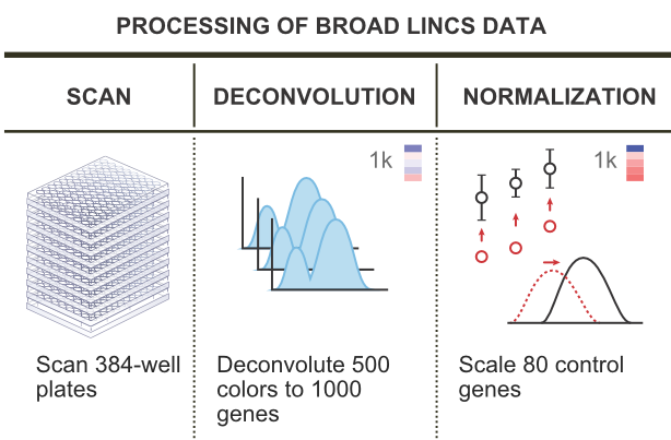
In order to facilitate statistical analysis on the L1000 data, the raw bead fluorescence measurements are combined and transformed. First, the measurements from many beads of the same color are deconvolved to assign expression values to the appropriate pair of genes. The data then goes through multiple normalization steps (Liu et al.,, 2015; Bolstad et al.,, 2003). First, a set of genes are identified as being stable across cell lines and perturbations, and these are used to inform a power law transformation of all gene values. The expression values are then quantile-normalized across sets of experiments to make the distribution of expression levels the same for all experiments. These steps are illustrated in Figure 1.

Figure 1: The L1000 data preprocessing pipeline. The raw data are first measured from the beads in the experiments. Next, the data from each color of bead are deconvolved to assign expression values to the two genes which share that bead color. Finally, the data are normalized to yield directly comparable data across experiments. Source: Broad Institute LINCS cloud website (http://lincscloud.org).

Although these data processing steps result in data that are more amenable to statistical analysis, we have found that the deconvolution step in particular introduces artifacts in the data. This can be seen when we look at multiple experiments on the same cell line with the same experimental conditions. If we look at a pair of genes that share a bead color and form a scatterplot of their values across many experiments, we see that these artifacts can take several forms.

First of all, two genes that are paired on the same bead color may not be expressed at levels such that they are easily distinguished. This can lead to assigning both genes the same value, resulting in a clustering of data directly on the $x=y$ diagonal. Secondly, the deconvolution step, which uses a simple $k$-means algorithm, can be misled if there are many beads sampled with very low fluorescence values. This, combined with the quantile normalization step, can lead to additional clusters that are not at the true expression value. Finally, the deconvolution step can result in assigning the expression levels of the genes incorrectly. That is, the expression level of gene A of the pair on the same bead color is sometimes assigned to gene B instead, and vice versa. Figure 2 shows examples of the raw bead data and illustrates the difficulty of the deconvolution step.

Figure 2: Example histograms of raw bead fluorescence values for single bead colors. The plot on the left shows an example where the two peaks corresponding to the genes sharing the bead color are relatively easy to distinguish. The right plot shows an example where the deconvolution is difficult.

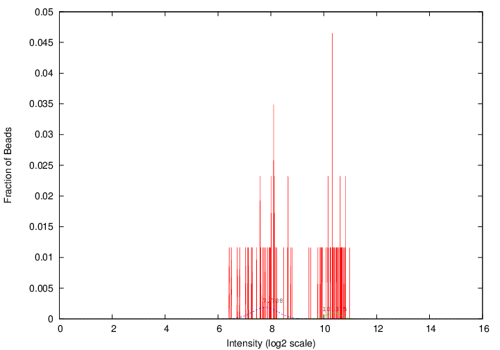
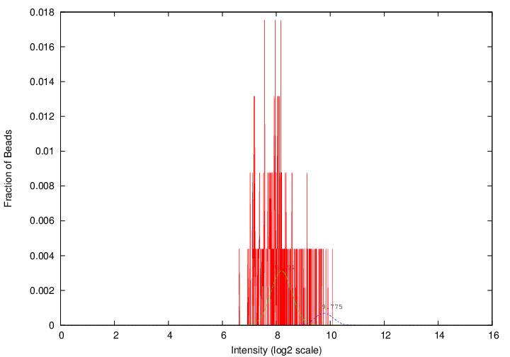
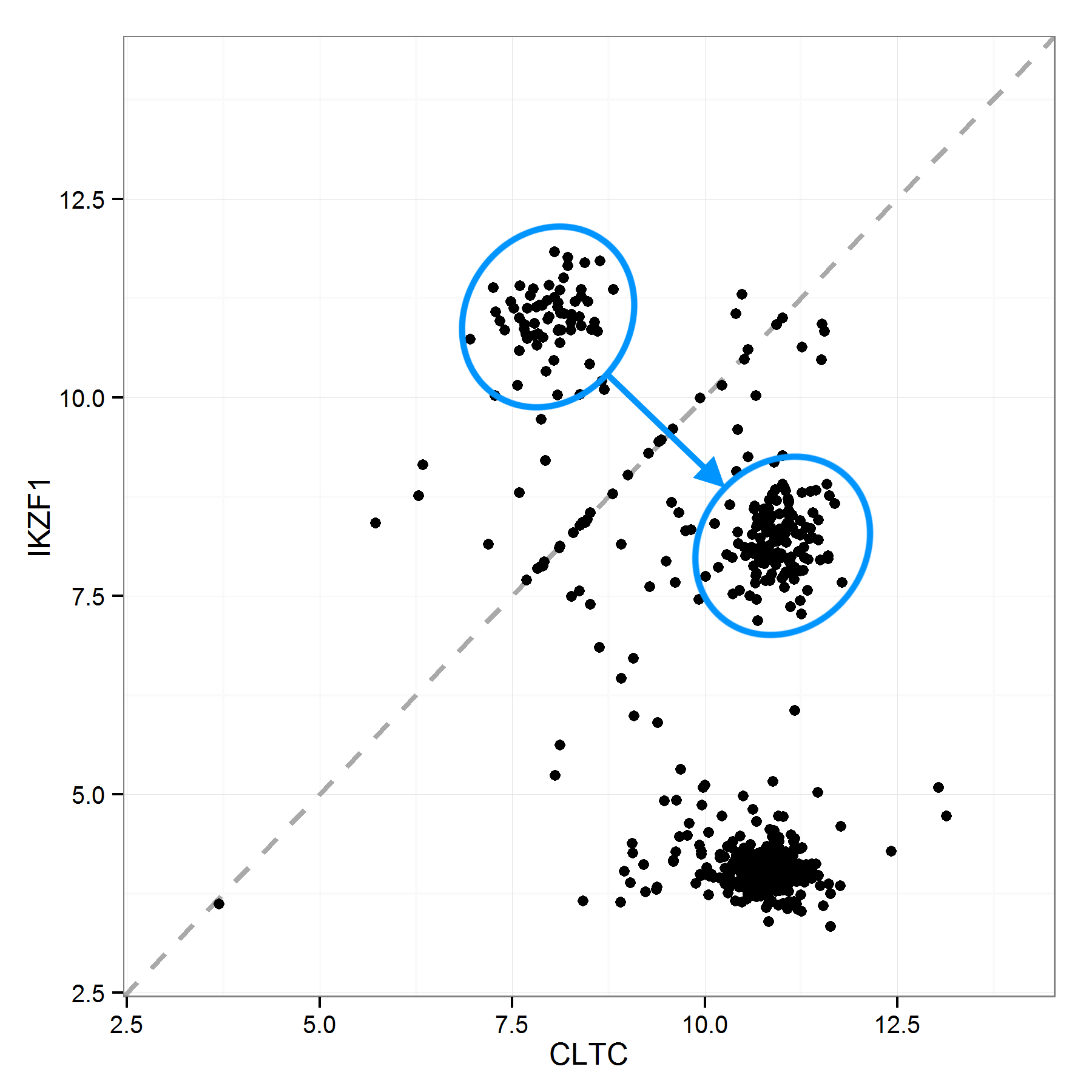
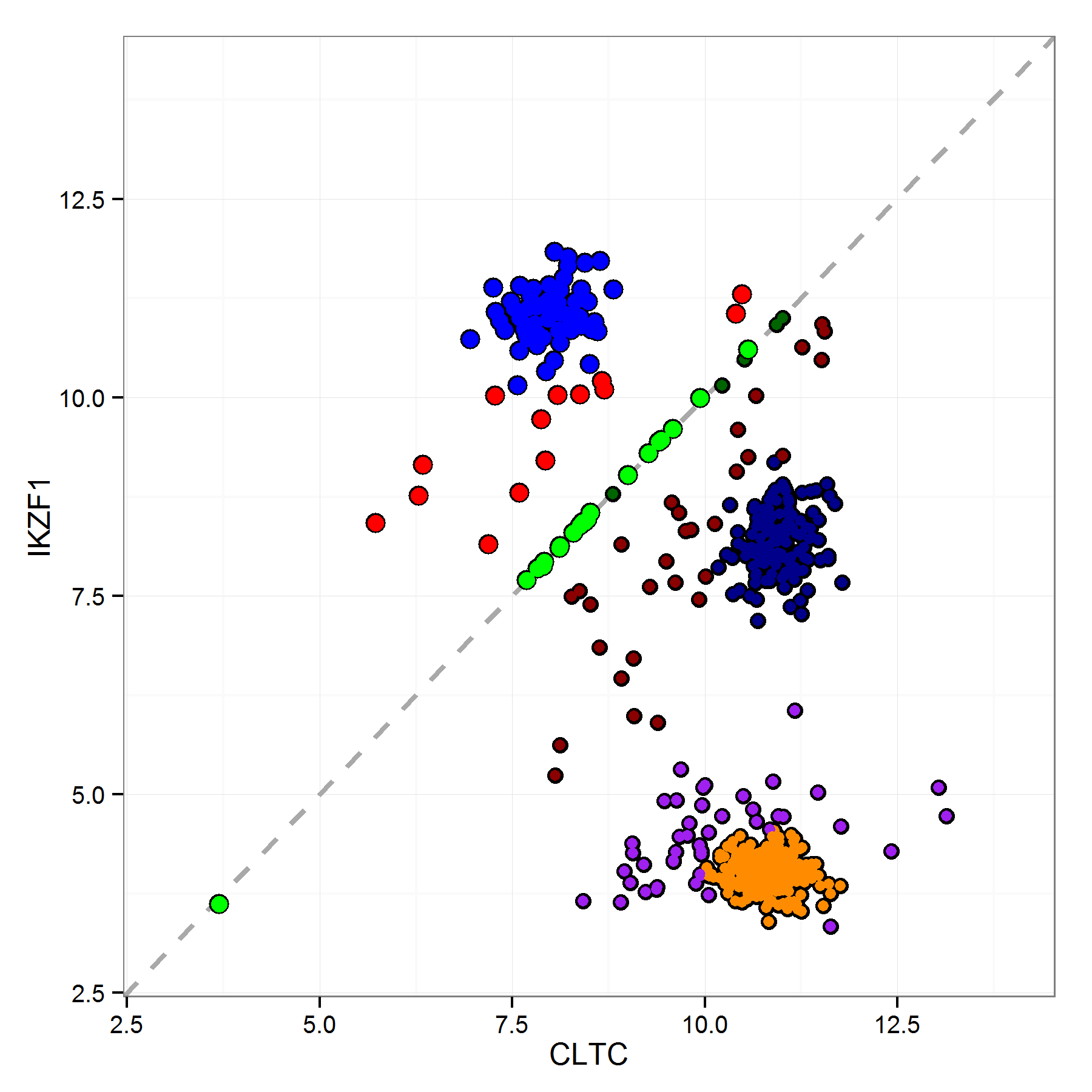
Figure 3 shows examples of these three types of artifact in the L1000 data. The figure shows the expression values for two paired genes, CTLC and IKZF1. Each point shows the values measured in a single experiment. All experiments in this dataset are on the same cell line, A375, and are untreated, used as controls. As such, we would expect a single cloud of observations centered around the point defined by the true expression values of the two genes. Instead, we see several clusters of observations, as well as points lying on or very near the diagonal. Note in particular the two circled sets of points. These appear to be a single cluster in which some of the points were flipped, with the expression values assigned to the wrong genes. If we flip one set of points across the diagonal, it falls directly on the other set. These phenomena occur with varying frequency across all the gene pairs.

Figure 3: Expression levels on a log-base-2 scale for two paired genes, CLTC and IKZF1, measured on the same bead, in the L1000 data. Data artifacts include points directly on the diagonal, multiple clusters rather than a single one as may be expected, and flipping between the two circled clusters of points, with the CLTC value incorrectly assigned to IKZF1, and vice versa. The blue arrow shows the effect of data correction using MCDC.

3 Method

We propose a method to detect and correct all three kinds of artifact present in the LINCS L1000 data: the multiple clusters introduced by the preprocessing pipeline, the erroneous assignment of the same expression value to paired genes, and flipping of the expression levels of paired genes. This improves the quality of the data and leads to better downstream analysis. We do this by looking at the data holistically rather than reprocessing the raw data, as in Liu et al., (2015). We adopt this holistic approach because some of the artifacts are likely to persist even if the deconvolution method is improved for individual gene pairs in isolation.

Our method is an extension of model-based clustering (Wolfe,, 1970; Banfield and Raftery,, 1993; McLachlan and Peel,, 2000; Fraley and Raftery,, 2002), which is a model-based method for finding clusters by fitting a multivariate Gaussian mixture model to the data. It has been found useful in many different contexts, including geochemical analysis (Templ et al.,, 2008), chemometrics (Fraley and Raftery,, 2007), and health studies (Flynt and Daepp,, 2015). This method is well adapted to estimating the expression levels because sometimes there are small groups of points not in the main cloud around the true value, such as the points on the diagonal in Figure 3. Model-based clustering can identify these groups as clusters and remove or downweight them, thus preventing them from contaminating the estimation of the gene expression levels.

However, while model-based clustering is able to identify the clusters as well as identifying outliers, it does not have a mechanism for identifying particular points as flipped. Here we extend the model-based clustering method to detect and take into account the flipping in the data. More generally, it can be used for data with any invertible transformation applied to a subset of the data. This extension allows us to use an Expectation-Maximization (EM) algorithm commonly used to estimate finite mixture models (Dempster et al.,, 1977; McLachlan and Krishnan,, 1997).

3.1 Model

Suppose we have some multivariate data, $\{\mathbf{x}_{i}:\;i=1,\dots,N$, generated by a finite mixture of $G$ distributions $f_{k}$, $k=1,\dots,G$ with probabilities $\tau_{1},\dots,\tau_{G}$:

$$f(\mathbf{x})=\sum_{k=1}^{G}\tau_{k}f_{k}(\mathbf{x}|\theta_{k}).$$

Suppose further that we do not observe $\mathbf{x}_{i}$, but rather $\mathbf{y}_{i}$, a possibly transformed version of $\mathbf{x}_{i}$, where the probability of a data point having been transformed can depend on the mixture component $k$ that $\mathbf{x}_{i}$ is drawn from:

$$\mathbf{y}_{i}=\left\{\begin{array}[]{ll}\mathbf{x}_{i}&\text{with probability }\pi_{k},\\ \mathbf{T}\mathbf{x}_{i}&\text{with probability }(1-\pi_{k}).\end{array}\right.$$

Here, $\mathbf{T}$ is any invertible transformation that preserves the domain of $\mathbf{x}$. Often, this may be represented as a matrix, but it may also be a functional transformation (i.e. a component-wise monotonic transformation). In the case of the L1000 data, this is just the $2\times 2$ matrix with zeros on the diagonals and ones on the off-diagonals, switching the two values.

Given the transformation $\mathbf{T}$, the distribution of $\mathbf{y}_{i}$ can be written as follows:

$$f(\mathbf{y}_{i}|\bm{\tau},\bm{\pi},\bm{\theta})=\sum_{k=1}^{G}\tau_{k}\left[\pi_{k}f_{k}(\mathbf{y}_{i}|\theta_{k})+(1-\pi_{k})f_{k}(\mathbf{T}^{-1}\mathbf{y}_{i}|\theta_{k})\right].$$

To simplify the notation, define $f_{ik}\equiv f_{k}(\mathbf{y}_{i}|\theta_{k})$ and $f^{-}_{ik}\equiv f_{k}(\mathbf{T}^{-1}\mathbf{y}_{i}|\theta_{k})$. Then the distribution of $\mathbf{y}_{i}$ can be written

$$f(\mathbf{y}|\bm{\tau},\bm{\pi},\bm{\theta})=\prod_{i=1}^{n}\sum_{k=1}^{G}\tau_{k}\left[\pi_{k}f_{ik}+(1-\pi_{k})f^{-}_{ik}\right].$$

3.2 EM Algorithm

We estimate this model by maximum likelihood using the EM algorithm. We formulate this as a missing data problem where the complete data are $\{\mathbf{y}_{i},\mathbf{z}_{i},\xi_{i}\}$. Here, $\mathbf{z}_{i}=(z_{i1},\dots,z_{iG})$ and $\xi_{i}$ are unobserved labels, with

$$z_{ik}=\left\{\begin{array}[]{ll}1&\text{if }\mathbf{y_{i}}\text{ belongs to group }k,\\ 0&\text{otherwise},\end{array}\right.$$

and

$$\xi_{i}=\left\{\begin{array}[]{ll}0&\text{if }\mathbf{y_{i}}\text{ has been transformed},\\ 1&\text{otherwise}.\end{array}\right.$$

Then the complete-data log-likelihood is

$$\ell(\bm{\theta},\bm{\tau},\mathbf{z},\bm{\pi},\bm{\xi}|\mathbf{y})=\sum_{i=1}^{n}\sum_{k=1}^{G}z_{ik}\left[\right.\xi_{i}\log\left(\pi_{k}\tau_{k}f_{ik}\right)+\left.(1-\xi_{i})\log\left((1-\pi_{k})\tau_{k}f^{-}_{ik}\right)\right].$$

We can also write down the joint distribution of $\mathbf{z}_{i}$ and $\bm{\xi}_{i}$ given $\mathbf{y}_{i}$ and $\bm{\theta}$:

$$f(\mathbf{z}_{i},\bm{\xi}_{i}|\mathbf{y}_{i},\bm{\theta})=\frac{1}{f(\mathbf{y}_{i}|\bm{\tau},\bm{\pi},\bm{\theta})}\prod_{k=1}^{G}\left[(\tau_{k}\pi_{k}f_{ik})^{\xi_{i}}\cdot(\tau_{k}(1-\pi_{k})f_{ik}^{-})^{(1-\xi_{i})}\right]^{z_{ik}}.$$ (3)

For the E-step of the algorithm, we need to calculate the expected complete-data log-likelihood, namely

$$Q(\bm{\theta}|\bm{\theta}^{*}) = E[\ell(\bm{\theta},\bm{\tau},\mathbf{z},\bm{\pi},\bm{\xi}|\mathbf{y})|\mathbf{y},\bm{\tau}^{*},\bm{\pi}^{*},\bm{\theta}^{*}],$$

$$= \sum_{i=1}^{n}\sum_{k=1}^{G}E[z_{ik}\xi_{i}|\mathbf{y},\bm{\tau}^{*},\bm{\pi}^{*},\bm{\theta}^{*}]\log\left(\pi_{k}\tau_{k}f_{ik}\right)+$$

$$E[z_{ik}(1-\xi_{i})|\mathbf{y},\bm{\tau}^{*},\bm{\pi}^{*},\bm{\theta}^{*}]\log\left((1-\pi_{k})\tau_{k}f^{-}_{ik}\right).$$

From Equation (3), we have

$$E[z_{ik}\xi_{i}|\mathbf{y},\bm{\tau}^{*},\bm{\pi}^{*},\bm{\theta}^{*}] = \frac{\tau_{k}^{*}\pi_{k}^{*}f_{ik}}{f(\mathbf{y}_{i}|\bm{\tau}^{*},\bm{\pi}^{*},\bm{\theta}^{*})},$$

$$E[z_{ik}(1-\xi_{i})|\mathbf{y},\bm{\tau}^{*},\bm{\pi}^{*},\bm{\theta}^{*}] = \frac{\tau_{k}^{*}(1-\pi_{k}^{*})f_{ik}^{-}}{f(\mathbf{y}_{i}|\bm{\tau}^{*},\bm{\pi}^{*},\bm{\theta}^{*})}.$$

We have $z_{ik}\xi_{i}+z_{ik}(1-\xi_{i})=z_{ik}$ and $\sum_{k=1}^{G}z_{ik}=1$. This leads to the following updates of the estimates of $z_{ik}$ and $\xi_{i}$, which make up the E-step:

$$\widehat{z}_{ik} = \frac{\tau_{k}^{*}[\pi_{k}^{*}f_{ik}+(1-\pi_{k}^{*}f_{ik}^{-})]}{f(y_{i}|\bm{\tau}^{*},\bm{\pi}^{*},\bm{\theta}^{*})},$$

$$\widehat{\xi}_{i} = \frac{\sum_{k=1}^{G}\tau_{k}^{*}\pi_{k}^{*}f_{ik}}{f(y_{i}|\bm{\tau}^{*},\bm{\pi}^{*},\bm{\theta}^{*})}.$$

The M-step is then as follows:

$$\widehat{\tau}_{k} \leftarrow \frac{n_{k}}{n},$$

$$\widehat{\pi}_{k} \leftarrow \frac{\sum_{i=1}^{n}\widehat{z}_{ik}\widehat{\xi}_{i}}{n_{k}},$$

$$\widehat{\bm{\mu}}_{k} \leftarrow \frac{\sum_{i=1}^{n}\widehat{z}_{ik}(\widehat{\xi}_{i}\mathbf{y}_{i}+(1-\widehat{\xi}_{i})\mathbf{T}^{-1}\mathbf{y}_{i})}{n_{k}},$$

$$n_{k} \equiv \sum_{i=1}^{n}\widehat{z}_{ik}.$$

To get the variance of the clusters, we follow the steps from Celeux and Govaert, (1995), modifying the within-cluster scattering matrix $W$ and the scattering matrix $W_{k}$ of cluster $k$ to be

$$W = \sum_{k=1}^{G}\sum_{i=1}^{n}\widehat{z}_{ik}\left[\widehat{\xi}_{i}(\mathbf{y}_{i}-\widehat{\bm{\mu}}_{k})(\mathbf{y}_{i}-\widehat{\bm{\mu}}_{k})^{\prime}+(1-\widehat{\xi}_{i})(\mathbf{T}^{-1}\mathbf{y}_{i}-\widehat{\bm{\mu}}_{k})(\mathbf{T}^{-1}\mathbf{y}_{i}-\widehat{\bm{\mu}}_{k})^{\prime}\right],$$

$$W_{k} = \sum_{i=1}^{n}\widehat{z}_{ik}\left[\widehat{\xi}_{i}(\mathbf{y}_{i}-\widehat{\bm{\mu}}_{k})(\mathbf{y}_{i}-\widehat{\bm{\mu}}_{k})^{\prime}+(1-\widehat{\xi}_{i})(\mathbf{T}^{-1}\mathbf{y}_{i}-\widehat{\bm{\mu}}_{k})(\mathbf{T}^{-1}\mathbf{y}_{i}-\widehat{\bm{\mu}}_{k})^{\prime}\right].$$

These can then be used to calculate $\Sigma_{k}$ under different variance models.

We iterate the EM steps until convergence, and this leads to a local optimum of the log-likelihood (Wu,, 1983). Although this is not guaranteed to be the global optimum, choosing starting values intelligently or doing multiple restarts have been shown to lead to good solutions (Fraley and Raftery,, 1998; Biernacki et al.,, 2003).

Our model assumes that each cluster variance is independent. We select the best number of clusters by running MCDC with the number of clusters ranging from 1 to some maximum number of clusters (9 in our case) and then comparing the BIC values for the resulting estimated models (Fraley and Raftery,, 2002).

For our gene expression data, we estimate the expression levels of a pair of genes as the mean of the largest cluster (the cluster with the most points assigned to it) found using the chosen model. This allows us to ignore the artifactual clusters that result from the preprocessing of the data in estimating the expression levels of the genes.

4 Simulation Study

We now describe a simulation study in which data with some of the key characteristics of the LINCS L1000 data were simulated. We simulated datasets with no clustering (i.e. one cluster), but where some of the observations were flipped. We also simulated datasets with clustering (two clusters), where some of the observations were flipped.

Finally, we simulated a dataset where no observations were flipped, but instead some observations were rotated and scaled. This is to show that the method can be effective when some of the data are perturbed in ways other than flipping.

4.1 Simulation 1: One Cluster With Flipping

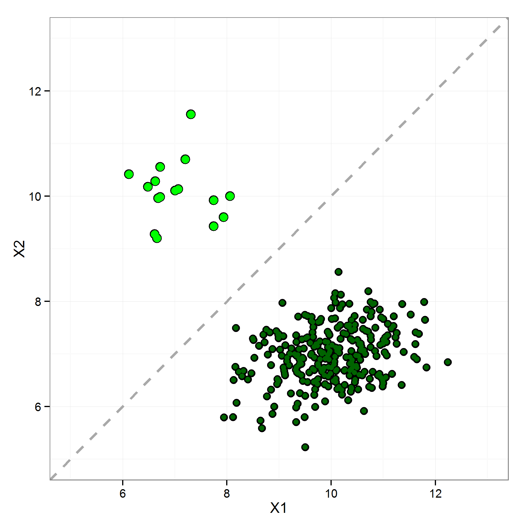
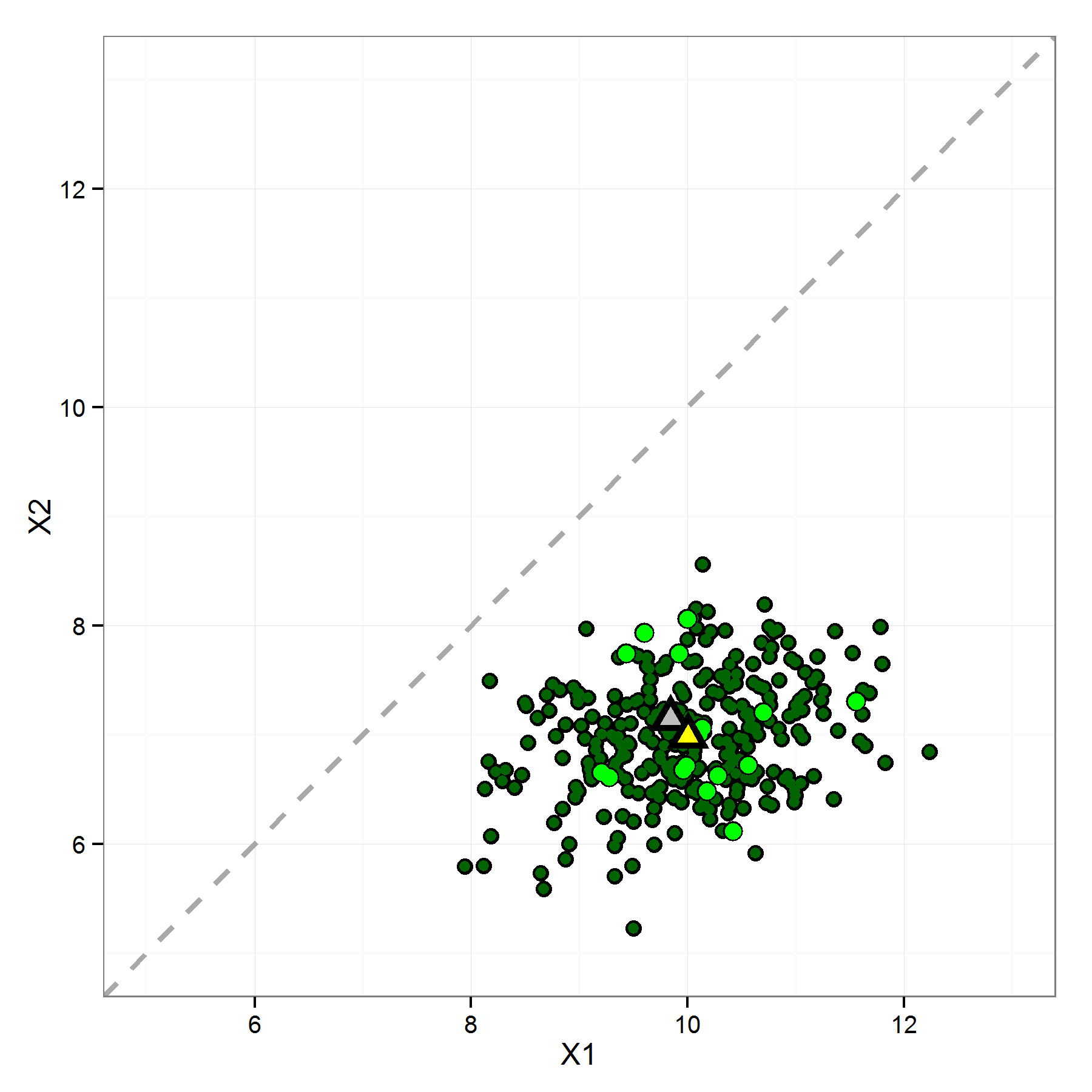
Figure 4 is an example dataset from our first simulation. This simulation represents what we see in the LINCS L1000 data in the best case, with no clustering or diagonal values (i.e. a single cluster), but with some flipping. For the simulation, we generated 100 datasets with 300 points each from the single cluster model with flipping probabilities $(1-\pi)$ of 0.05 to 0.45 in increments of 0.05. We applied MCDC to each simulated dataset and counted the number of times the correct number of clusters (one) was selected as well as the percentage of the points correctly identified as flipped or not. Finally, we looked at the inferred gene means compared to taking the mean of the data without MCDC.

The correct number of clusters (i.e. one) was selected for all but one of the 900 datasets, and in the one erroneous dataset out of 900 only a few points were in a second cluster. In 858 of the 900 datasets no errors were made - all the points were correctly identified as being flipped or not flipped. In three datasets, all with the highest probability of flipping, namely 0.45, all the points were misidentified by being flipped to the wrong side, while in one dataset (again with $\pi=0.55$), a single large cluster with no flipping was identified. The remaining 38 datasets had one to three points out of 300 misidentified. All these misidentifications make sense, since we expect rare cases where a point crosses the $x=y$ line as well as cases where more points are flipped when using a flipping probability near 0.5.

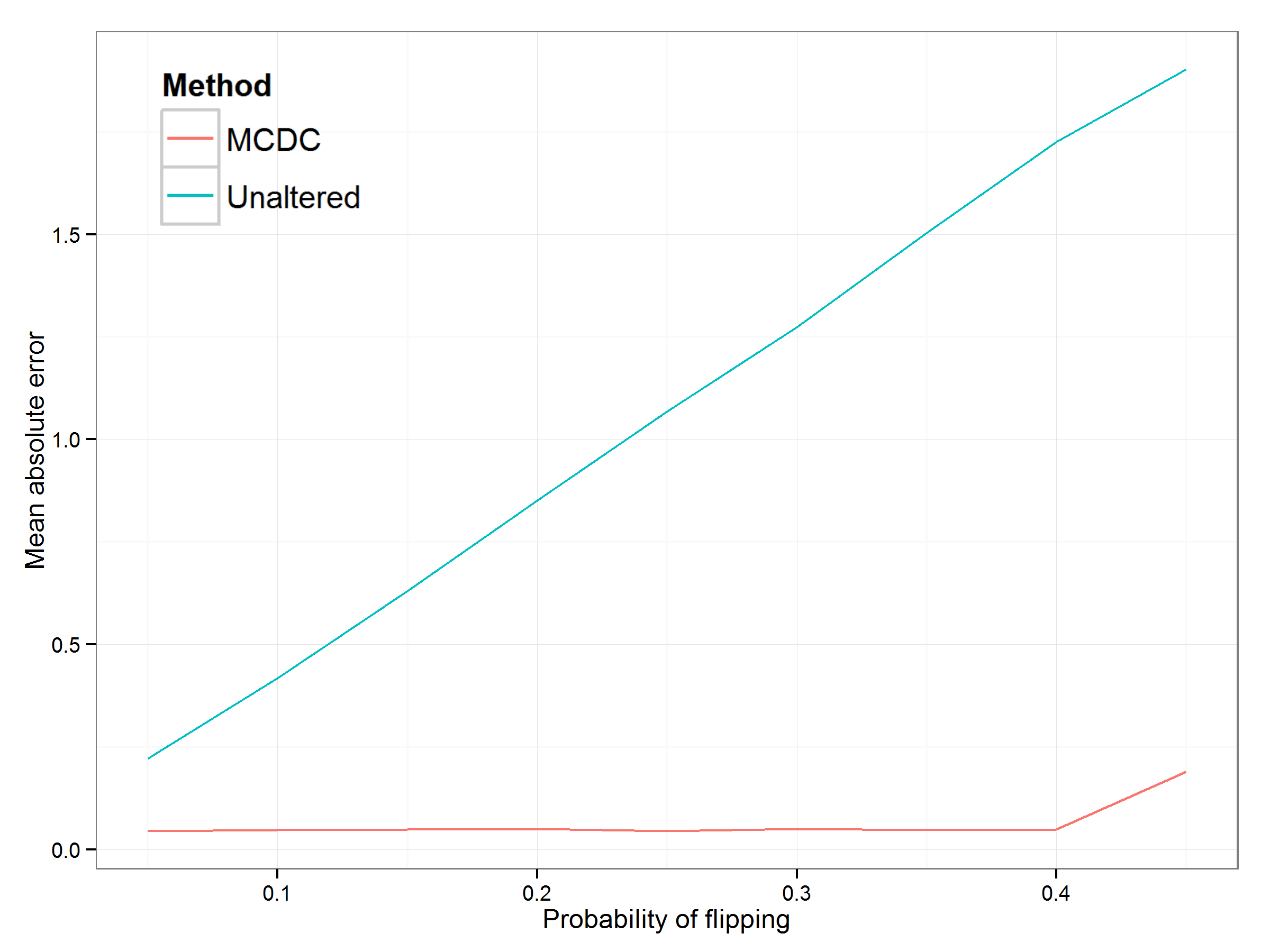
Figure 5 and Table 1 show the mean absolute error in inferred mean using MCDC versus the unaltered data. For each flipping probability, we calculated the mean absolute error of the inferred mean from the true mean. MCDC did much better than taking the unaltered mean in all cases, improving on the unaltered data by a factor of 5 to 36, depending on the probability of flipping.

Figure 4: One Dataset from Simulation 1: One Cluster with Flipping. Left panel: Original data with flipped data points. Right panel: Data after correction by MCDC. MCDC identified and corrected all the flipped points. The grey triangle is the mean of all the data, and the yellow triangle is the mean of the data after correction by MCDC.

Figure 5: Simulation 1: Mean Absolute Error in Inferred Mean. The blue line is using unaltered data, while the red line is using the mean of the largest cluster found by MCDC.

Table 1: Simulation 1: Mean Absolute Error (MAE) in Inferred Mean for Unaltered data and MCDC-corrected Data, as the probability of flipping increases. The MAE ratio is the ratio of mean absolute error using the unaltered data divided by the MAE using the MCDC-corrected data. Values greater than 1 indicate improvement by using MCDC.

Probability of	Unaltered	MCDC	MAE
Flipping	MAE	MAE	Ratio
0.05	0.22	0.04	5
0.10	0.42	0.05	9
0.15	0.63	0.05	13
0.20	0.85	0.05	17
0.25	1.07	0.05	24
0.30	1.27	0.05	25
0.35	1.50	0.05	32
0.40	1.73	0.05	36
0.45	1.90	0.19	10

4.2 Simulation 2: Two Clusters with Flipping

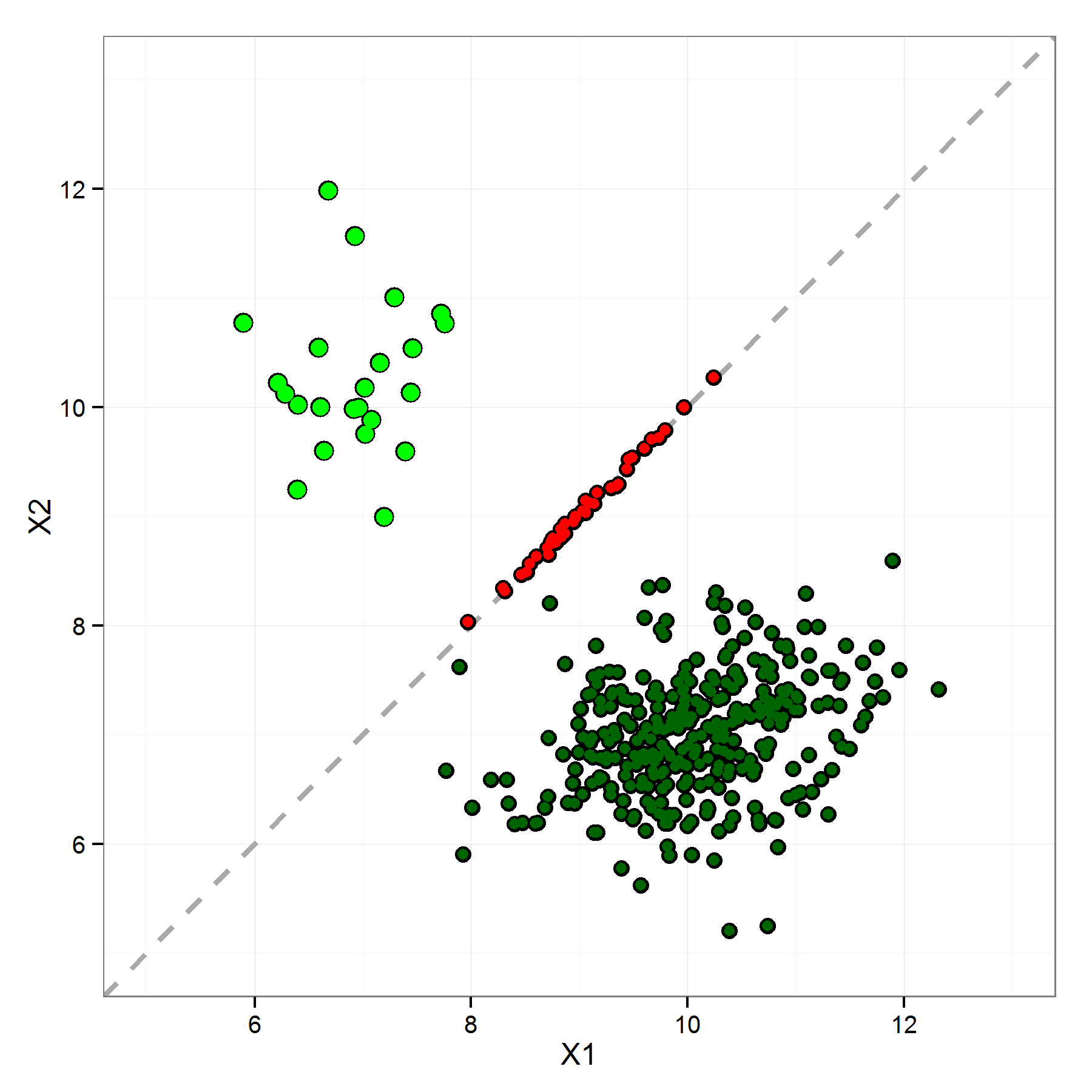
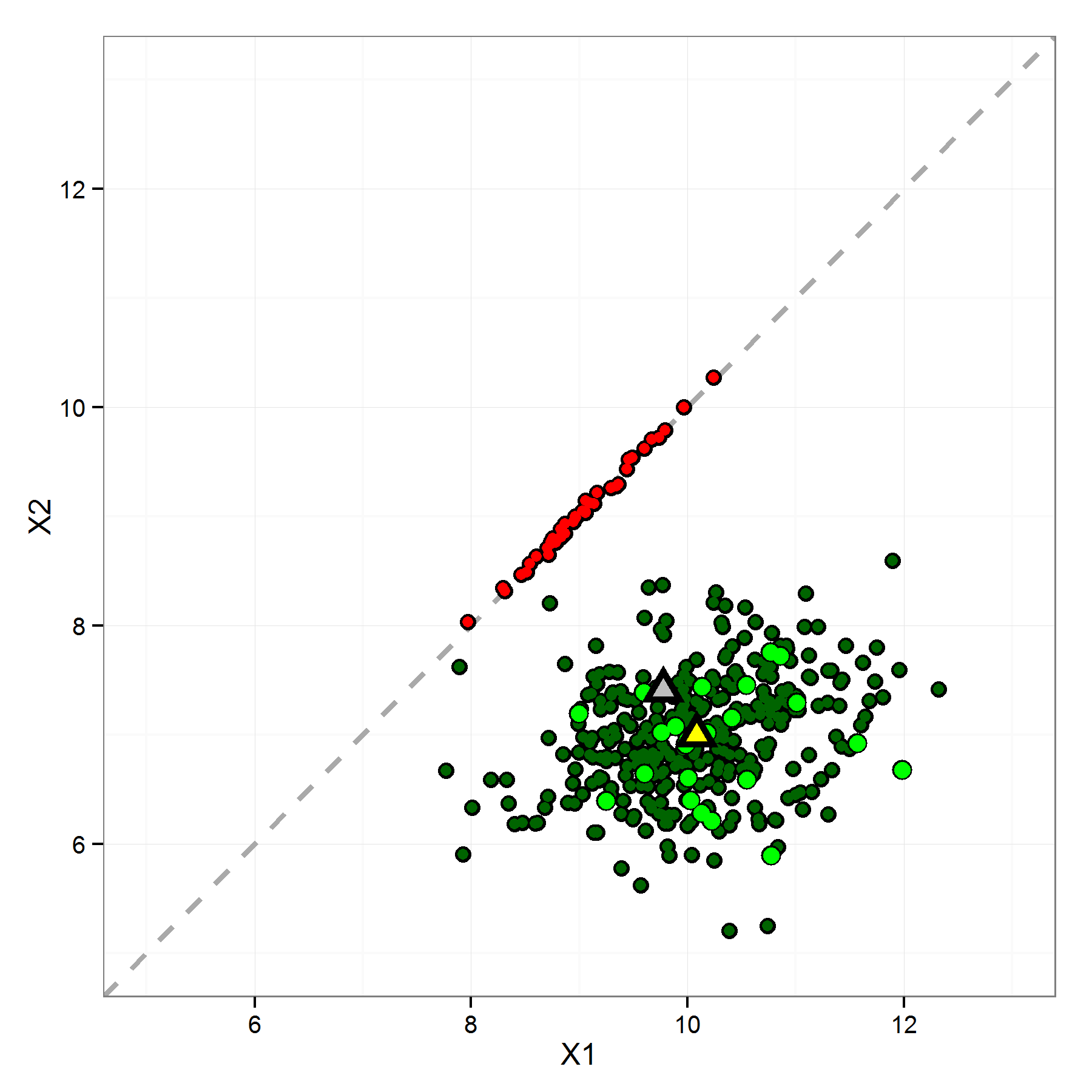
For the second simulation, we added a second cluster on the diagonal, as demonstrated in Figure 6. This reflects a common issue we see in the L1000 data. When the data processing pipeline has trouble differentiating between the two gene expression levels, it can end up assigning them both the same value. For these data, we wanted to see how well MCDC identified the “good” points (not the diagonal cluster). Again, we used the mean of the largest cluster as the inferred mean. For the simulation, we generated 100 datasets with 400 points each for the two-cluster model with flipping probabilities $(1-\pi)$ of 0.05 to 0.45, and probability $\tau$ of a point being in the true cluster 0.55 to 0.95, in increments of 0.05.

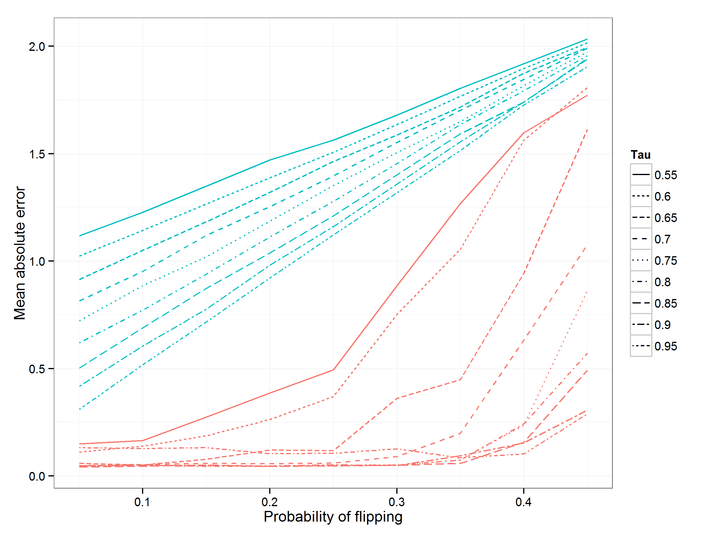
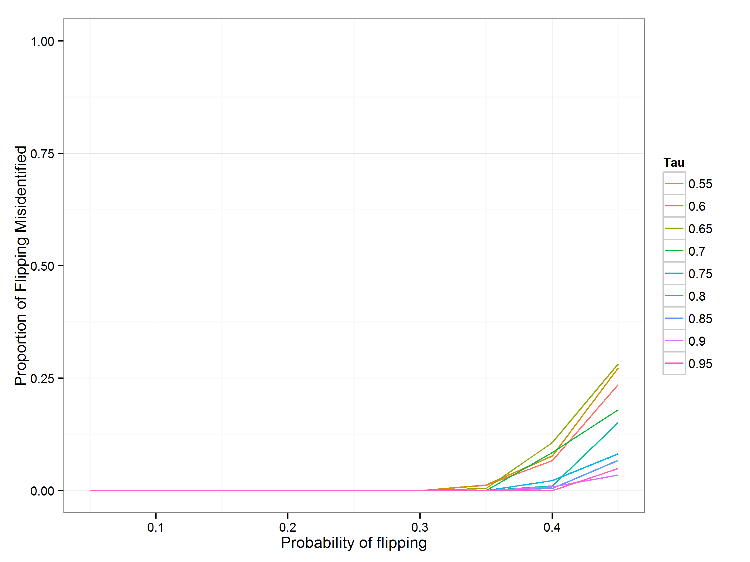
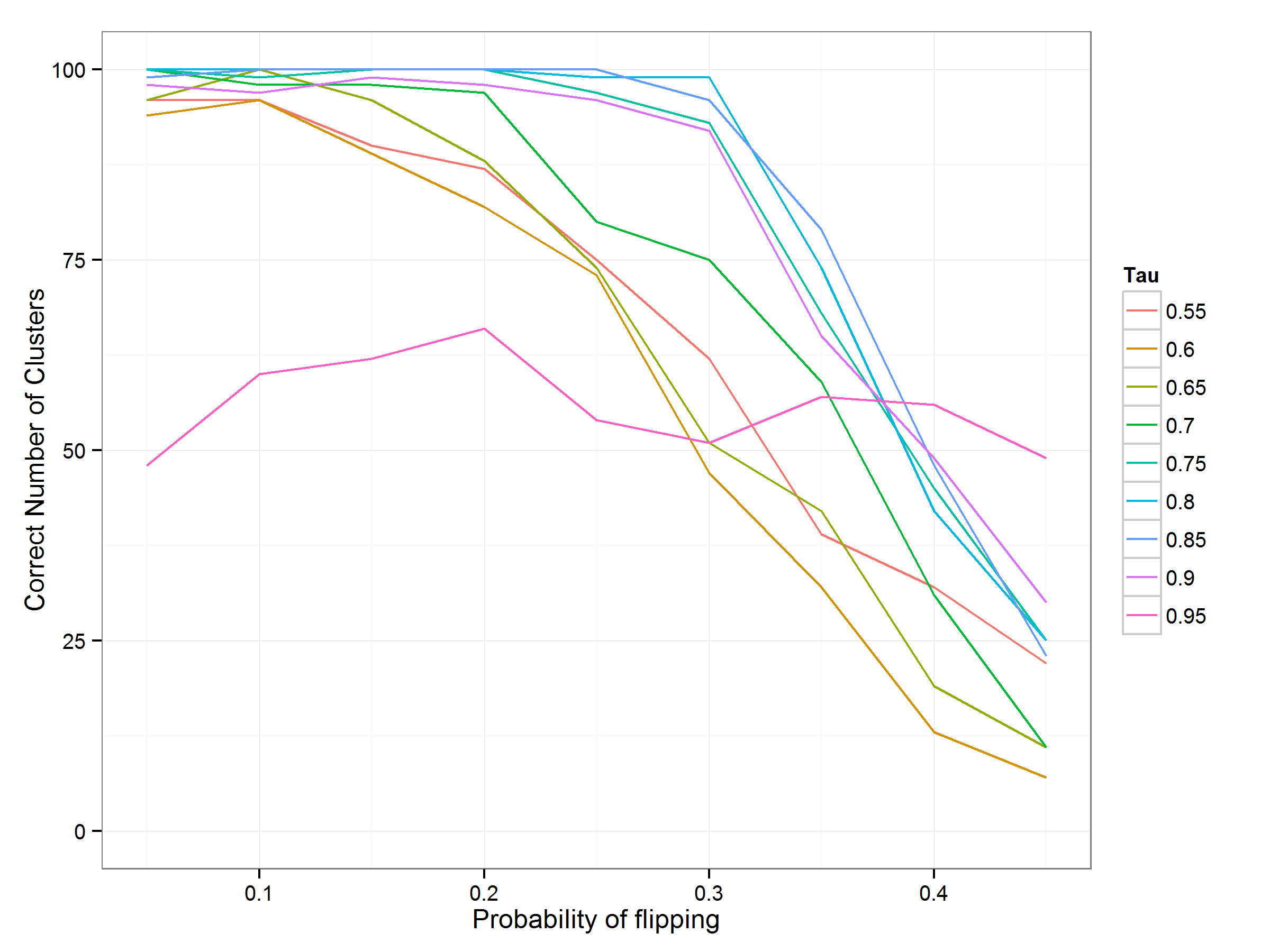
Figure 7 shows the comparison of mean absolute error in the inferred mean. The MCDC results are better across the board, although we see that as $\tau$ decreases, it is more likely to find the diagonal cluster as the largest one. Figure 8 shows that MCDC does well in identifying which points are flipped or not. In Figure 9, we see that the correct number of clusters is not generally identified as well as we might like. This may be due to poor initialization of the algorithm and may be corrected with multiple random initializations.

Figure 6: Simulated dataset 2: 2 clusters after flipping. MCDC correctly identifies the two clusters and the flipped points, as seen in the plot on the left. The grey triangle is the mean of all the data, which is moved from its true position due to the second cluster. The yellow triangle is the mean of the largest cluster found by MCDC and is much closer to the true value.

Figure 7: Mean absolute error in inferred mean comparison for simulation 2 when varying $\tau$, the probability that a point comes from the primary cluster. The blue line is using unaltered data, while the red line is using the mean of the largest cluster found by MCDC.

Figure 8: Proportion of points correctly identified as flipped or not flipped for simulation 2 when varying $\tau$, the probability that a point comes from the primary cluster. When there is a high probability of flipping (near 0.5), there may be more points in the flipped cluster, leading to MCDC identifying it as the main cluster and thus misidentifying all points for a particular dataset.

Figure 9: Number of datasets (out of 100) which identify 2 clusters as the best result for simulation 2 when varying $\tau$, the probability that a point comes from the primary cluster. When $\tau$ is high, MCDC may not identify the cluster on the diagonal properly due to the low number of points in that cluster.

4.3 Simulation 3: Three Clusters With Rotation and Scaling

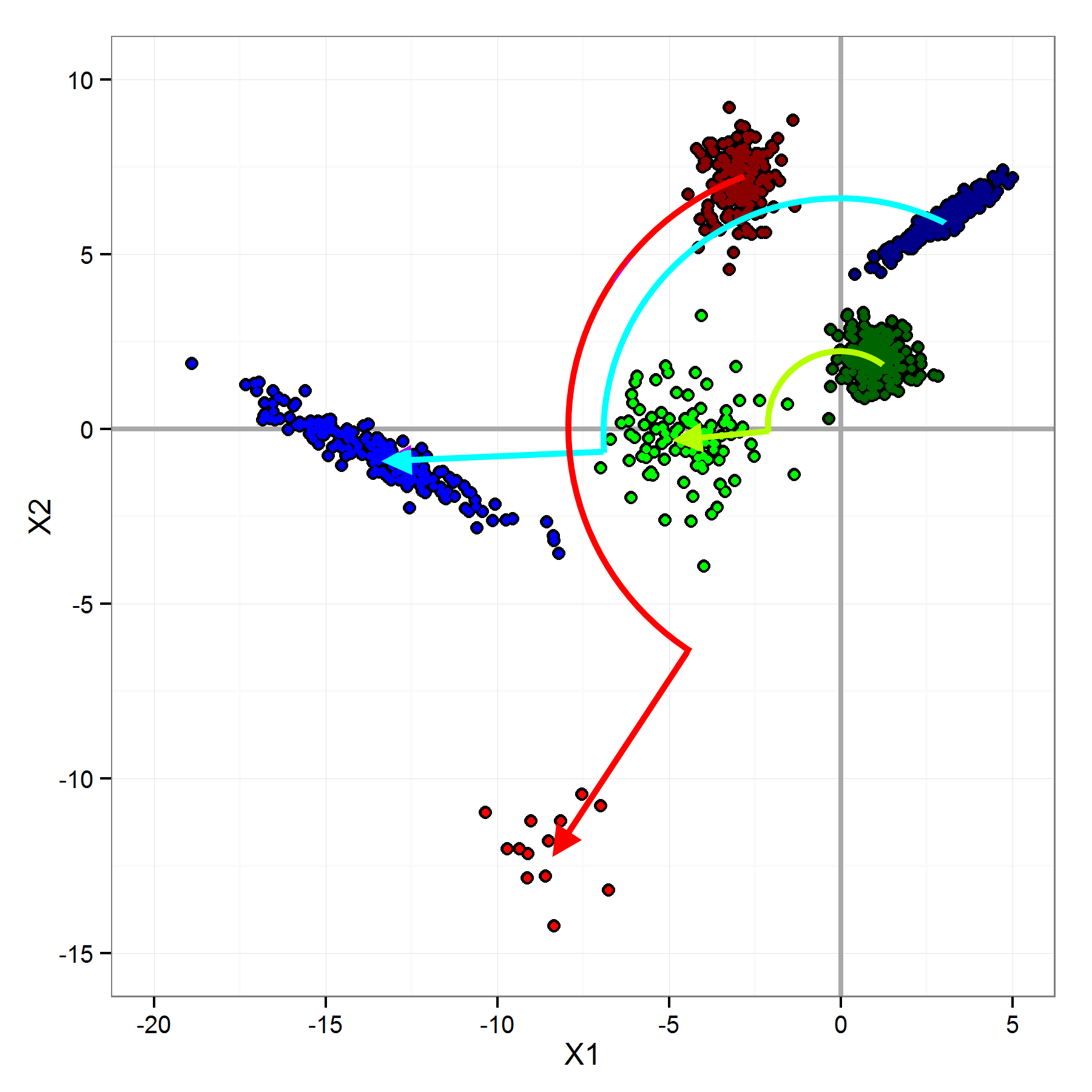
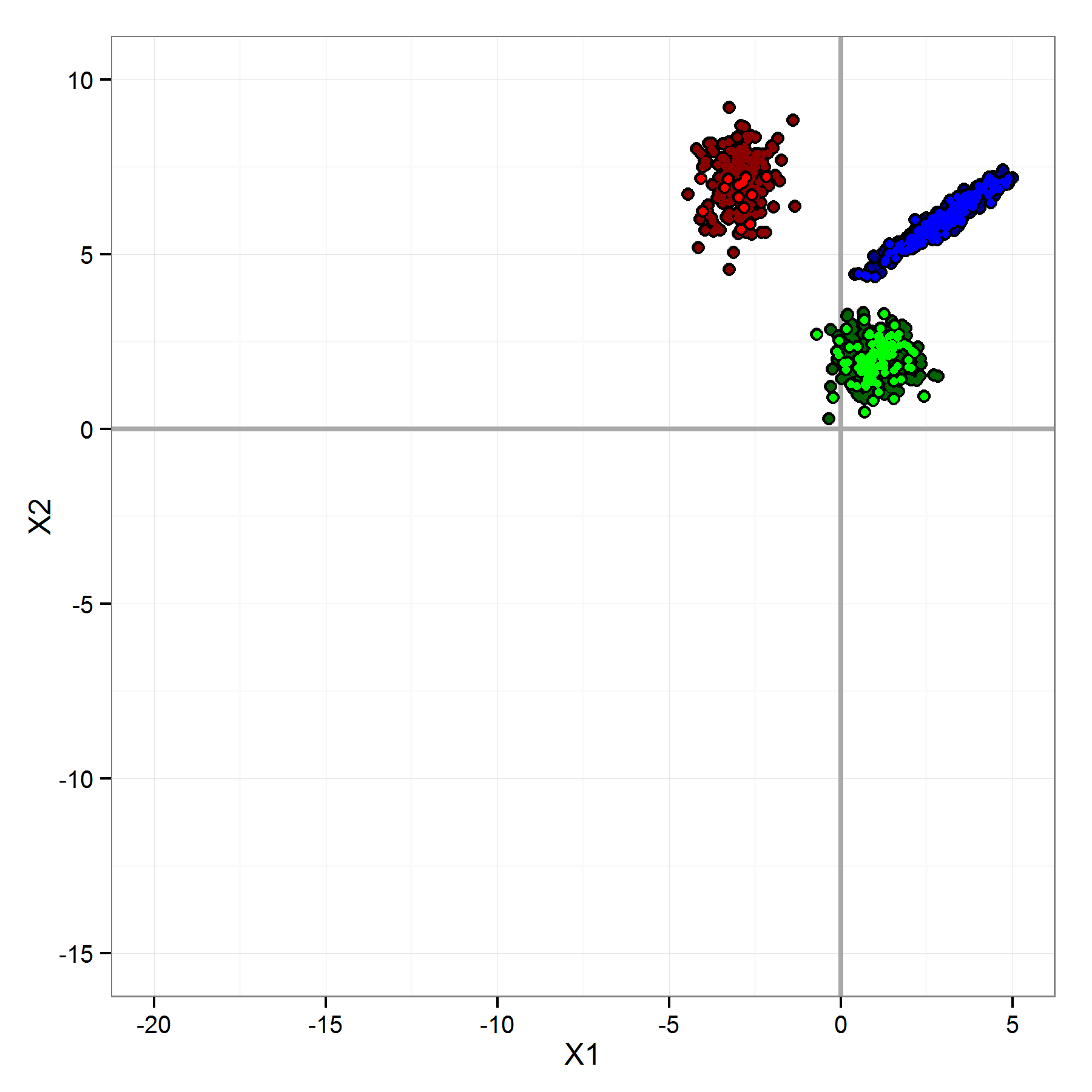
To show that MCDC can be applied to other kinds of data errors than flipping, we also generated a dataset with three clusters where the error process rotates and scales the data points affected. In this more complex situation, we used $n=1000$ points split among the three clusters with varying probabilities of transformation. MCDC selected the correct number of clusters and correctly classified all the points. Figure 10 shows the original and MCDC-corrected data. One caveat is that here, as in the flipping situation, the data error process was known to the MCDC algorithm.

Figure 10: Simulation dataset 3: 3 clusters with rotation and scaling. A data point is transformed by rotating it $120^{\circ}$ counter-clockwise around the origin and then scaling out from the origin by a factor of 2, as seen in the plot on the right. MCDC is able to identify the correct clusters and assign the transformed points back into the appropriate clusters, as on the left.

5 Application to LINCS L1000 Data

We applied MCDC to a portion of the LINCS L1000, namely the data from cell line A375, a human skin malignant melanoma cell line. We chose this cell line because it has good coverage in the L1000 data in terms of the number of different perturbations applied. We looked at improvement of the data in aggregate as well as improvement in a specific inferential setting.

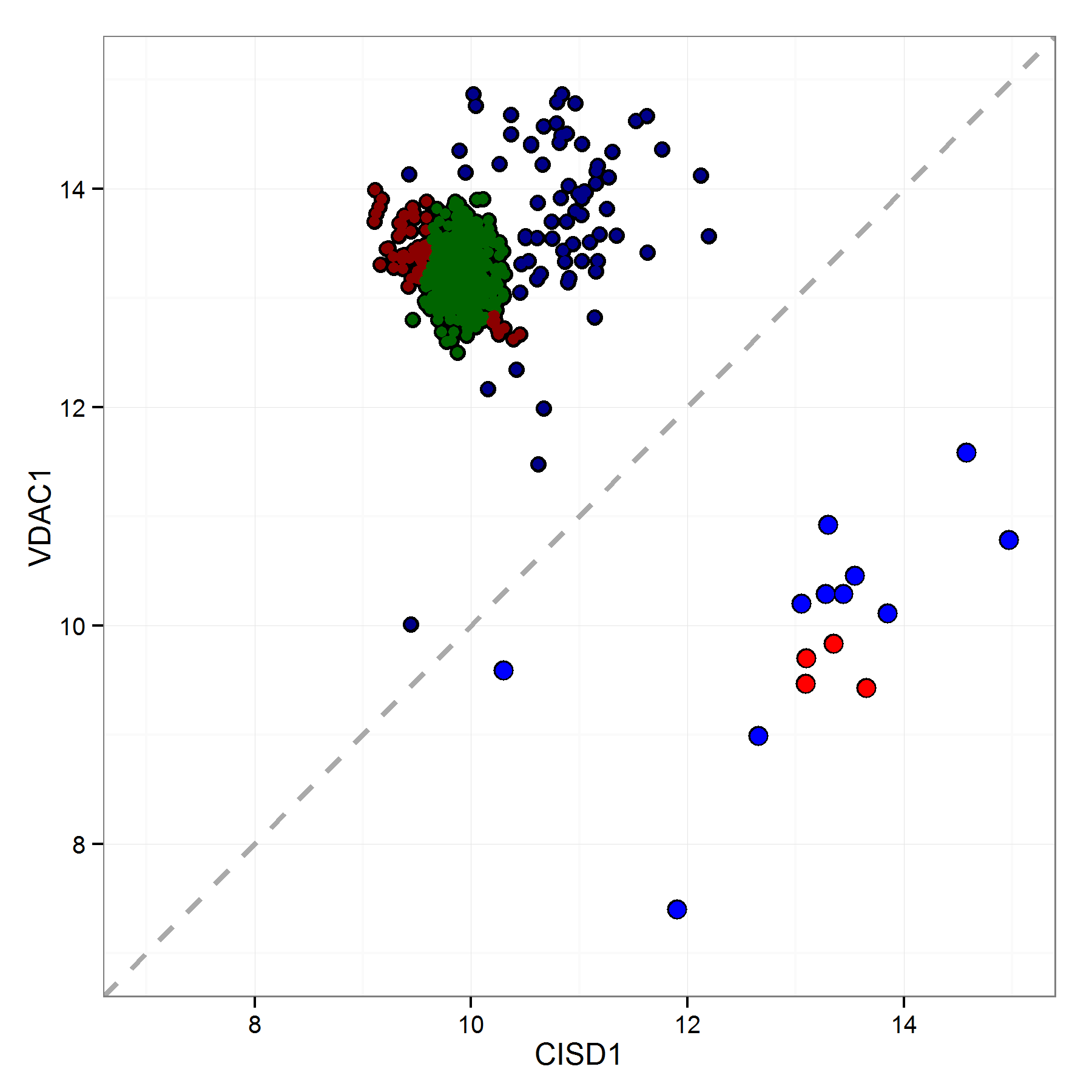
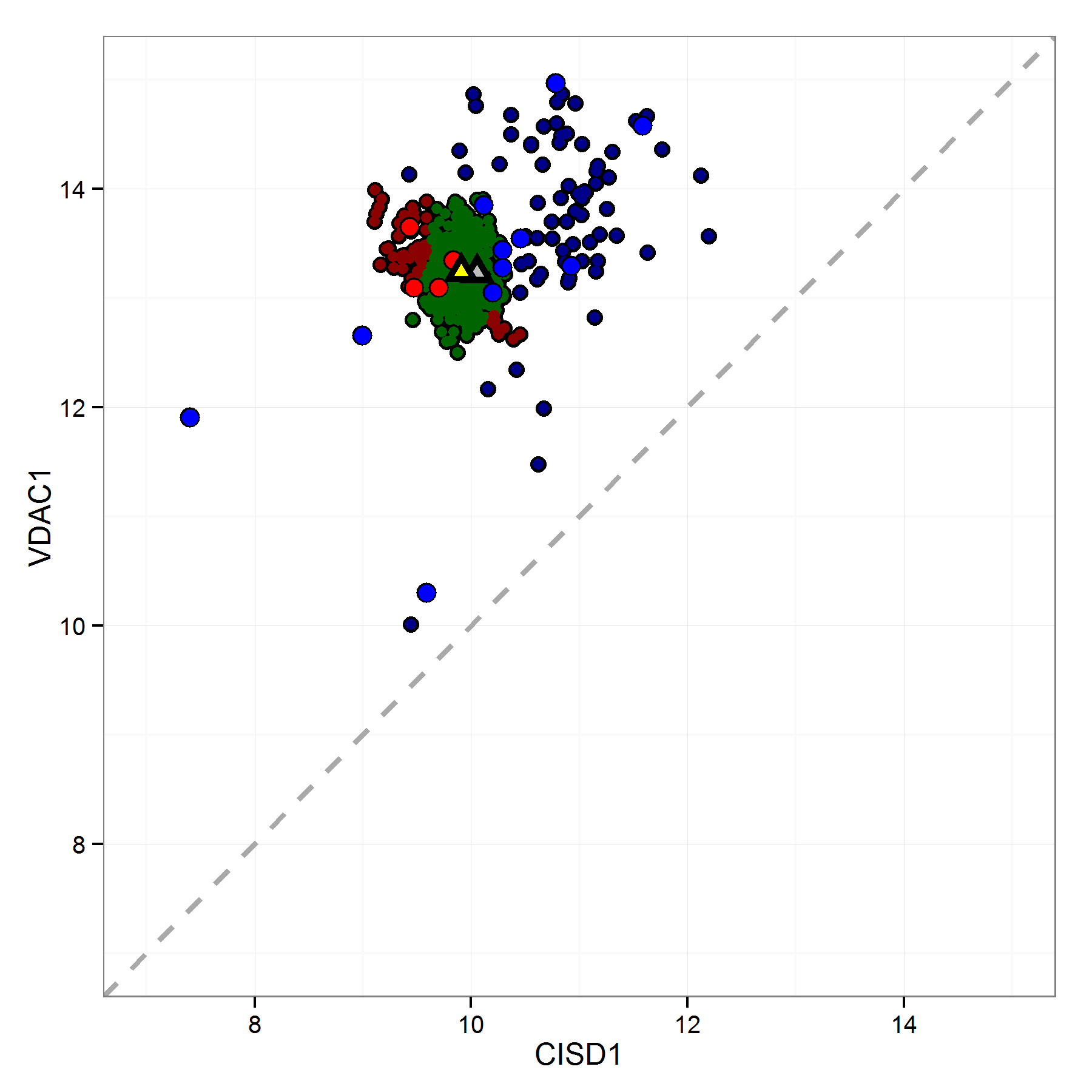
Figure 11 shows the results of applying MCDC to one gene pair in untreated experiments on cell line A375. Each point corresponds to a single experiment, and most of the points fall in the same region. However, there are a few points which appear to be mirrored across the $x=y$ line, and we suspect that these points have had the expression levels of the two genes switched. MCDC corrects these points and we see that they do indeed fall within the main body of points.

Figure 11: Example 1 showing results of applying MCDC to L1000 data. On the left is the data before correction, and on the right is that data after correction. Triangles indicate inferred mean - gray is the mean of all the data while yellow is the mean of the largest cluster found by MCDC.

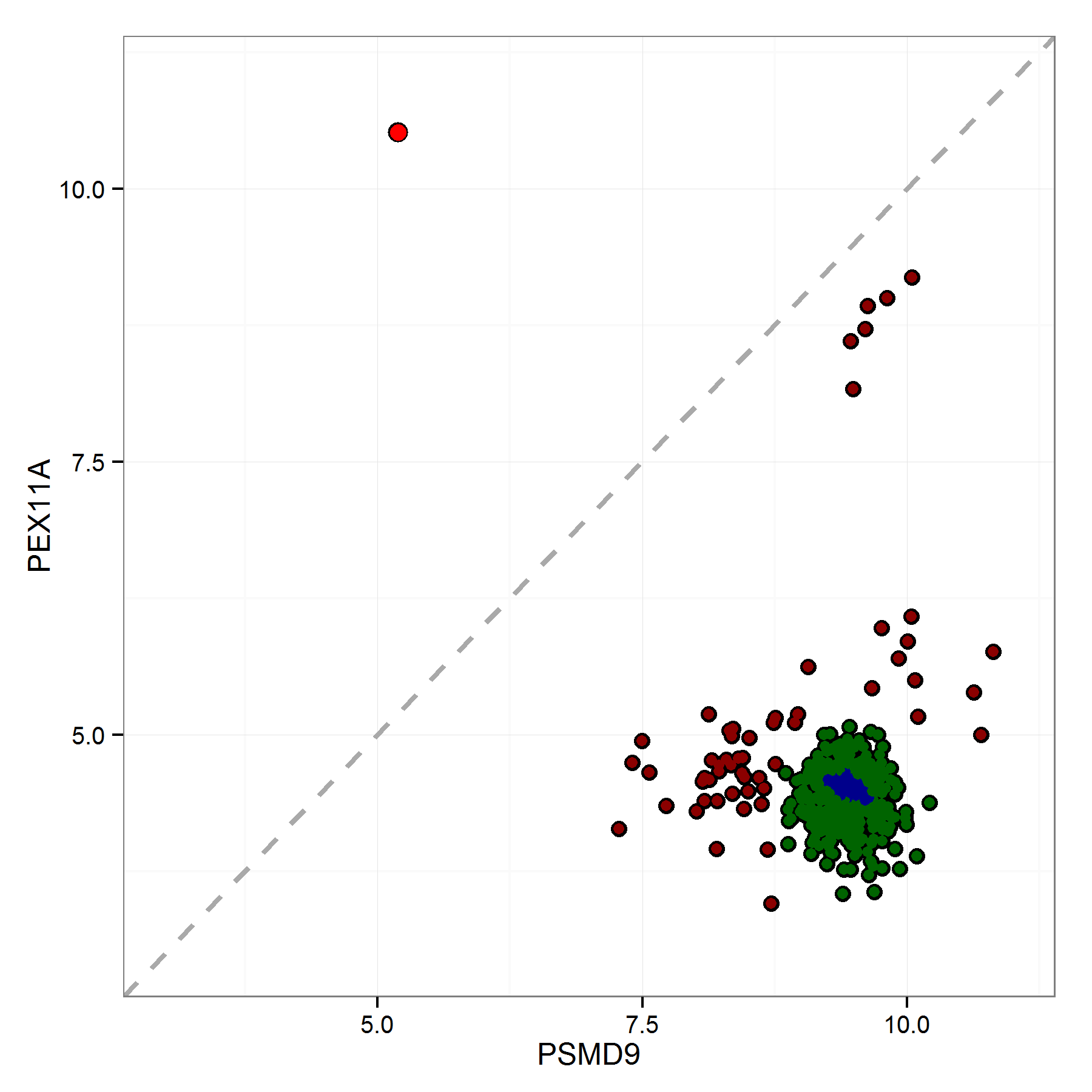
Note that here the best solution involves three components. This means that the distribution of the points may not be strictly normal, but the components overlap such that they form one contiguous cluster.

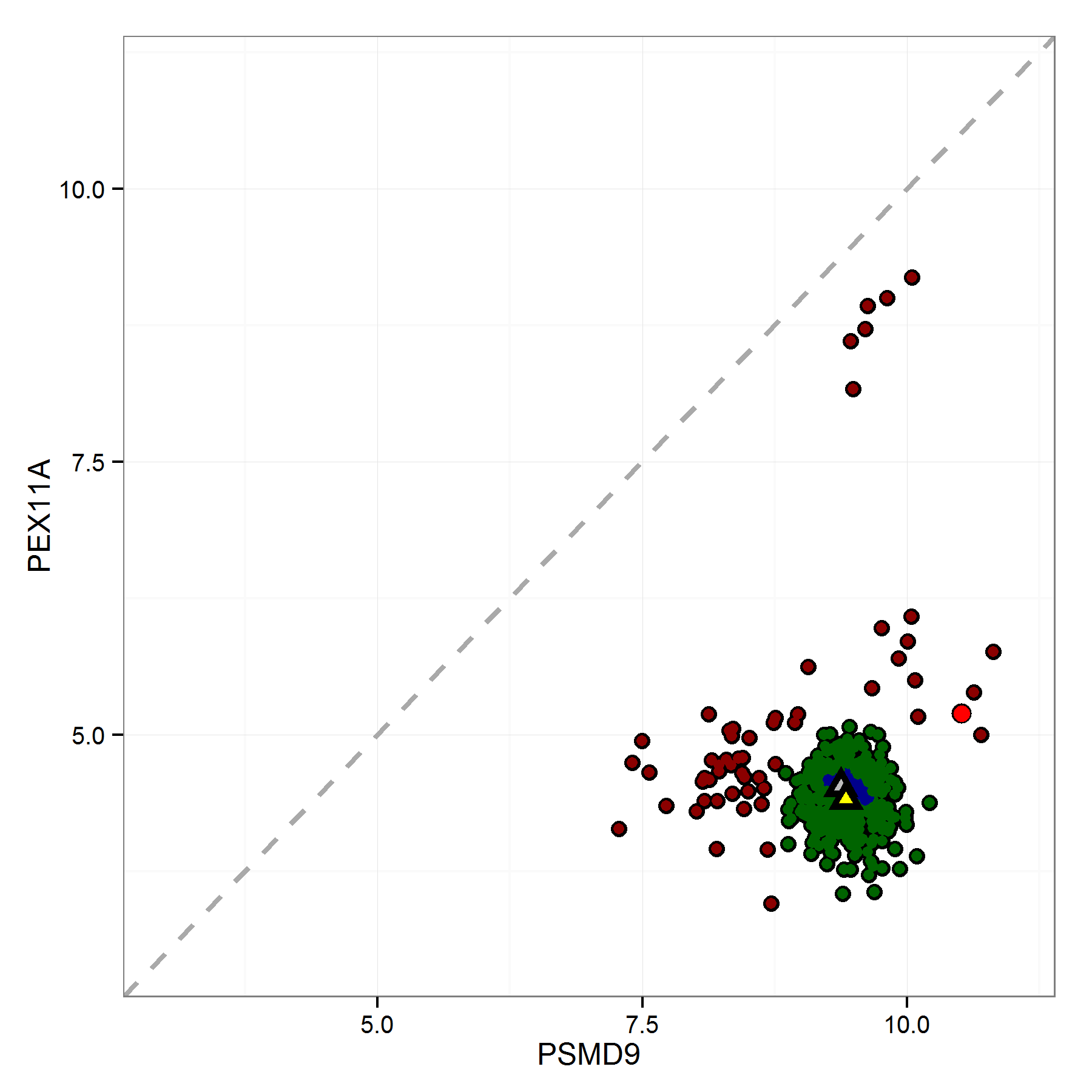
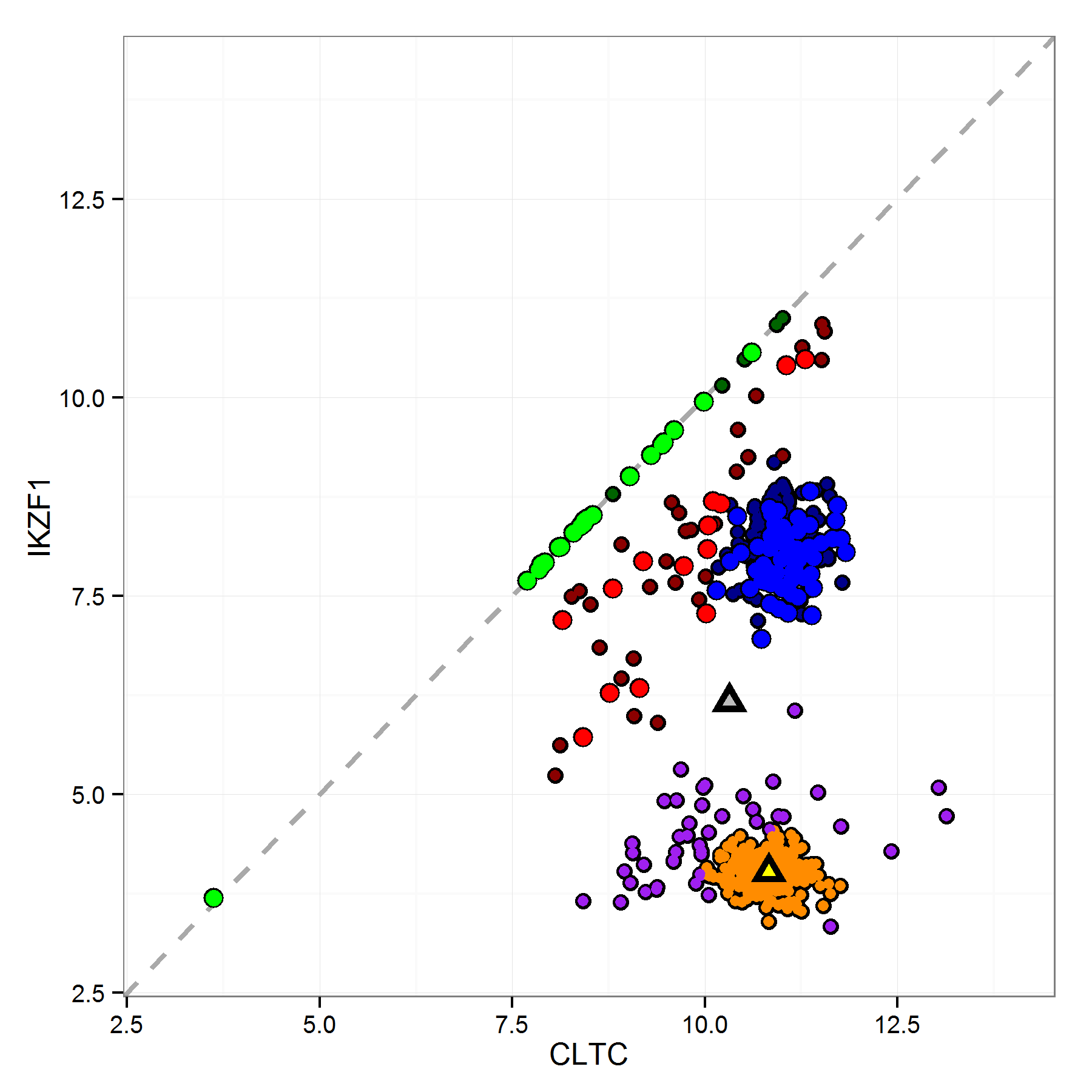
Figures 12 and 13 show MCDC applied to additional gene pairs in the same dataset. In each case MCDC succeeded in removing the artifacts in the data.

Figure 12: Example 2 showing results of applying MCDC to L1000 data. On the left is the data before correction, and on the right is that data after correction. Triangles indicate inferred mean - gray is the mean of all the data while yellow is the mean of the largest cluster found by MCDC.

Figure 13: Example 3 showing results of applying MCDC to L1000 data. On the left is the data before correction, and on the right is that data after correction. Triangles indicate inferred mean - gray is the mean of all the data while yellow is the mean of the largest cluster found by MCDC.

5.1 Agreement with External Baseline Data

First of all, we wanted to see if MCDC improves the data relative to an external baseline. There are about 2,000 untreated experiments in the A375 cell line. These experiments should all yield similar expression levels since they are all done under the same experimental conditions. We can get an estimate of the gene expression level of a particular gene by taking the mean across all the experiments. We refer to this as the unaltered data.

There are two expression level baseline datasets included in the LINCS L1000 metadata for cell line A375, one using RNAseq technology and the other using Affymetrix microarray technology. Each of these data were generated using an independent technology and can be compared to the values in the L1000 data. Since the baseline datasets are produced using different technologies, the scales of the expression levels are different than that from the L1000 data. In order to take this difference into account, we looked at the mean squared error (MSE) from a simple linear regression of the baseline data on the inferred gene expression levels from the L1000 data.

We then applied MCDC to see if this improved the estimates of gene expression. To do this, we applied MCDC separately to each pair of genes that were measured using the same bead color. For a gene pair, we ran MCDC on the data from the 2,000 experiments. Doing this for all 500 gene pairs, we ended up with an estimated gene expression level for all of the 1,000 landmark genes. These estimates were also compared to the baseline estimates and we were able to compare the MSEs of the unaltered data with those from the corrected data. Note particularly in Figure 13 that the inferred mean after MCDC is substantially different than the mean of the full dataset, moving it from a location not near any data to within the largest cluster.

Table 2 shows the results of this analysis. Using the corrected data improved the MSE by 8% when using the Affymetrix data and by 7% when using the RNAseq data.

Table 2: MSE of regressing external baseline data on imputed gene means. Comparison of unaltered means and MCDC data. Affymetrix and RNAseq baselines both are from external sources independent of the LINCS L1000 data.

	Affymetrix	RNAseq
Method	Baseline	Baseline
Unaltered	1.91	1.66
MCDC	1.76	1.55

5.2 Gene Regulatory Network Inference

As well as improving the overall estimates of gene expression levels, MCDC identifies particular experiments where the gene pairs are flipped. This improvement of the data leads to improvements in methods that use the data in a more granular way.

To see this improvement, we looked at inferring gene regulatory networks from the LINCS L1000 data. We looked at knockdown experiments, which target a specific gene to suppress its expression level. This target gene is the regulator in these experiments, and the remaining genes are potential targets, giving us a causal pathway by which to infer networks.

We developed a simple posterior probability approach using the knockdown data to infer edges. To do this, we first standardized the knockdown data using the untreated experiments on the same plate to get $z$-values. We then used a simple linear regression model, regressing each potential target on the knocked down gene. This can be converted into a posterior probability of there being an edge from the knocked-down gene to the target gene. This approach is fast and allows us to incorporate prior probabilities as well. The final result is a ranked edgelist.

The LINCS L1000 data includes multiple knockdown experiments for most of the landmark genes. We used the posterior probability method on the knockdown experiments for cell line A375 to generate a ranked list of potential edges. In order to assess the results, we used a gene-set library compiled from TRANSFAC and JASPAR (Wingender et al.,, 2000; Sandelin et al.,, 2004) and accessed from Enrichr at http://amp.pharm.mssm.edu/Enrichr/ (Chen et al.,, 2013). This is a list of transcription factors, namely genes that are known to control the expression levels of other genes. Each transcription factor has a list of target genes, yielding an assessment edgelist.

The TRANSFAC and JASPAR (T&J) edgelist is not a complete reference since not all gene relationships are captured in the T&J library. This is partially because the T&J data focuses on transcription factors but also because the true regulatory networks are not fully known. The T&J edgelist includes edges for 37 transcription factors also found among the LINCS landmark genes. This includes approximately 4,200 regulator-target pairs out of about 42,000 potential edges for which we computed posterior probabilities.

To see the effect of MCDC, we applied the posterior probability method using the unaltered data and compared the results with using the same posterior probability method on the data after it had been corrected using MCDC. This results in two ranked lists of gene pairs with associated posterior probabilities. We compare these with the T&J assessment dataset by taking all edges with a posterior probability over a specified cutoff and creating two-by-two tables showing how well the truncated edgelists overlap with the T&J edgelist

Table 3 shows the two-by-two tables generated at posterior probability cutoffs of 0.5 and 0.95. We also report approximate $p$-values by using the probability of getting at least the number of true positives found using a binomial($n$, $p$) distribution, where $n$ is the number of pairs in the inferred list and $p$ is the probability of selecting a true edge from the total number of possible edges. From the table, we can see that the $p$-value is better for the corrected data at both probability cutoffs. The corrected data includes more edges at both cutoffs but maintains a similar precision, the proportion of edges which are true edges.

Table 3: 2x2 tables for cell line A375 using knockdown experiments for finding edges. Compared to TRANSFAC and JASPAR from Enrichr. When using the unaltered data and looking at edges with posterior probability of 0.5 or greater, 41 of the 302 candidate edges are found in TRANSFAC and JASPAR, and 14 of the 81 candidate edges at a cutoff of 0.95 are true edges. Similarly, when using the MCDC-corrected data, 63 of the 463 candidate edges at a cutoff of 0.5 are true edges and 20 of the 119 at a cutoff of 0.95 are true edges. Approximate binomial p-values included.

			T&J
			cutoff: 0.5			cutoff: 0.95
			Yes	No		Yes	No
	Unaltered	Yes	41	261		14	67
		No	4152	38836		4179	39030
			p-value: 0.02			p-value: 0.02
	MCDC	Yes	63	400		20	99
		No	4130	38697		4173	38998
			p-value: 0.004			p-value: 0.01

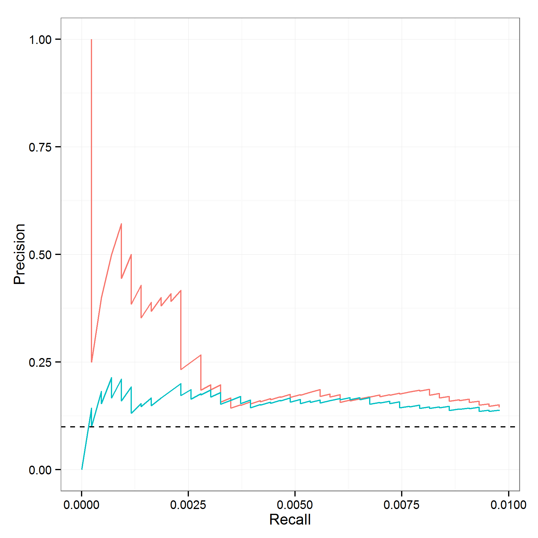
Another way of looking at the results is via the precision-recall curve (Raghavan et al.,, 1989). Precision and recall are both calculated by truncating our ranked list of edges and looking only at the edges in the truncated list. Precision is the proportion of the edges in the truncated list which are true edges. Recall is the proportion of all true edges which are in the truncated list. The precision-recall curve takes a ranked list of edges from a procedure and shows how the precision varies as more and more edges are included from that list. High precision at low recall indicates that the procedure is good at identifying true edges at the highest probability. This is important in many cases, particularly genetic studies, because it gives researchers good information on where to focus their efforts in subsequent studies.

Figure 14 compares the precision-recall curves for the unaltered and corrected data at the very top of the edgelist. The dashed line shows what would be expected by randomly ordering the edges, and above that line is an improvement. Both methods are improvements, but the corrected data yields much better results for the very top edges returned. This is of particular importance for further research because having high confidence in the top edges allows the biologist to develop further experiments to focus on these edges in additional, more targeted experiments. In this respect, data correction with MCDC provides substantial improvement.

We can see this by looking at the inferred edges, ranked so that the first edge has the highest posterior probability, the second has the second highest, and so one. Table 4 is constructed by ranking the edgelist from the posterior probability method on a particular dataset. Thus the first edge in the list is that with the highest posterior probability, the second edge has the next highest posterior probability, and so on. We then look at each edge and see if it also is found in the T&J assessment edgelist. The rank in the table indicates the position at with the $n$-th edge in T&J was found in the ranked edgelist. So the edge with highest posterior probability using the MCDC-corrected data is in T&J, as is the edge with the 5th highest posterior probability, etc. Only one of the top 10 edges from the unaltered data is a true edge, while 5 of the top 10 edges from the MCDC-corrected data are true edges.

Figure 14: Precision-recall curve comparing edgelists from unaltered (blue line) and MCDC-corrected (red line) data on knock down data.

Table 4: Comparison of the rank of the first 5 edges found that match the TRANSFAC and JASPAR edgelist. Edges ranked by posterior probability. MCDC-corrected data produces found edges at higher ranks than the uncorrected data. See text for explanation of how the table was constructed.

Found Edge	Unaltered Rank	MCDC Rank
1	7	1
2	11	5
3	14	6
4	19	7
5	26	10

6 Discussion

When working with any data, understanding the unique aspects of how it was generated and processed can be helpful in developing models and methods, leading to improved inference. This is particularly true with genomic data. There are often many steps of data transformation and normalization between the raw measured data and what is used by the researcher in drawing conclusions (Binder and Preibisch,, 2008). When these steps are not known or understood, assumptions about sources of error can be misinformed and lead to degraded performance in inference. Price et al., (2006) identified population stratification of allele frequency in disease studies, while Gomez-Alvarez et al., (2009) found that a particular sequencing technique resulted in many artificial replicates. Lehmann et al., (2013) showed that quantile normalization of microarray data introduced a phase shift into time-series in strains of cyanobacteria, changing night-expressed genes into day-expressed genes and vice versa. Stokes et al., (2007) developed a tool to identify and remove artifacts in genomic data. Batch effects have been identified as a significant source of systematic error that can be corrected (Leek et al.,, 2010; Chen et al.,, 2011; Sun et al.,, 2011). Identifying these sources of error is crucial, and in some cases can lead to vastly improved results.

We showed how understanding the data-processing pipeline of the LINCS L1000 data allowed us to identify the introduction of a particular error, namely the flipping of expression values for gene pairs. This led to the development of MCDC, which is able to identify and correct these flipping errors. We were able to apply MCDC to improve the L1000 data in aggregate, as measured against external standards. This improvement of the data also led to improved inference of regulatory relationships between the genes, in particular for the edges ranked highest. Moreover, the use of the EM algorithm for optimization makes MCDC fast and useful for large datasets.

MCDC is an extension of model-based clustering, which has been extensively used in other analyses of genetic data, including sequence analysis (Verbist et al.,, 2015) and image analysis of microarrays (Li et al.,, 2005). One of the most common uses of model-based clustering in genetics is in finding meaningful groups among gene expression profiles across multiple experiments under different experimental conditions (cell sources, phases, applied drugs, etc.) (Siegmund et al.,, 2004; Jiang et al.,, 2004). This includes methods using Gaussian mixture models (Yeung et al.,, 2001), infinite mixture models (Medvedovic and Sivaganesan,, 2002) and Bayesian hierarchical clustering (Cooke et al.,, 2011). Our use of MCDC as a step in improving data quality is complementary to these analysis methods.

We showed in our simulation experiments that MCDC is able to accurately identify the data points which have been altered and thus improve the quality of the data. It is not limited to flipping as seen in the LINCS data, but is able to handle any dataset where a subset of the data points have been altered in a known way. One possible extension of this method would be to compare different possible data transformations to identify which is most compatible with the observed data.

References

- Ball et al., (2002) Ball, C. A., Sherlock, G., Parkinson, H., Rocca-Sera, P., Brooksbank, C., Causton, H. C., Cavalieri, D., Gaasterland, T., Hingamp, P., Holstege, F., et al. (2002). Standards for microarray data. Science, 298:539–539.
- Banfield and Raftery, (1993) Banfield, J. D. and Raftery, A. E. (1993). Model-based Gaussian and non-Gaussian clustering. Biometrics, 49:803–821.
- Bansal et al., (2006) Bansal, M., Della Gatta, G., and Di Bernardo, D. (2006). Inference of gene regulatory networks and compound mode of action from time course gene expression profiles. Bioinformatics, 22:815–822.
- Basso et al., (2005) Basso, K., Margolin, A. A., Stolovitzky, G., Klein, U., Dalla-Favera, R., and Califano, A. (2005). Reverse engineering of regulatory networks in human B cells. Nature Genetics, 37:382–390.
- Biernacki et al., (2003) Biernacki, C., Celeux, G., and Govaert, G. (2003). Choosing starting values for the EM algorithm for getting the highest likelihood in multivariate Gaussian mixture models. Computational Statistics and Data Analysis, 41:561–575.
- Binder and Preibisch, (2008) Binder, H. and Preibisch, S. (2008). “Hook”-calibration of Genechip-microarrays: Theory and algorithm. Algorithms for Molecular Biology, 3:1–25.
- Bolstad et al., (2003) Bolstad, B. M., Irizarry, R. A., Åstrand, M., and Speed, T. P. (2003). A comparison of normalization methods for high density oligonucleotide array data based on variance and bias. Bioinformatics, 19:185–193.
- Celeux and Govaert, (1995) Celeux, G. and Govaert, G. (1995). Gaussian parsimonious clustering models. Pattern Recognition, 28:781–793.
- Chen et al., (2015) Chen, B., Greenside, P., Paik, H., Sirota, M., Hadley, D., and Butte, A. (2015). Relating chemical structure to cellular response: An integrative analysis of gene expression, bioactivity, and structural data across 11,000 compounds. CPT: Pharmacometrics & Systems Pharmacology, 4:576–584.
- Chen et al., (2011) Chen, C., Grennan, K., Badner, J., Zhang, D., Gershon, E., Jin, L., and Liu, C. (2011). Removing batch effects in analysis of expression microarray data: an evaluation of six batch adjustment methods. PloS one, 6:e17238.
- Chen et al., (2013) Chen, E. Y., Tan, C. M., Kou, Y., Duan, Q., Wang, Z., Meirelles, G. V., Clark, N. R., and Ma’ayan, A. (2013). Enrichr: interactive and collaborative HTML5 gene list enrichment analysis tool. BMC Bioinformatics, 14:article 128.
- Cooke et al., (2011) Cooke, E. J., Savage, R. S., Kirk, P. D., Darkins, R., and Wild, D. L. (2011). Bayesian hierarchical clustering for microarray time series data with replicates and outlier measurements. BMC Bioinformatics, 12:article 399.
- Crick and others, (1970) Crick, F. and others (1970). Central dogma of molecular biology. Nature, 227:561–563.
- Dempster et al., (1977) Dempster, A. P., Laird, N. M., and Rubin, D. B. (1977). Maximum likelihood for incomplete data via the EM algorithm (with discussion). Journal of the Royal Statistical Society, Series B, 39:1–38.
- D’haeseleer et al., (1999) D’haeseleer, P., Wen, X., Fuhrman, S., Somogyi, R., et al. (1999). Linear modeling of mRNA expression levels during CNS development and injury. In Pacific Symposium on Biocomputing, volume 4, pages 41–52. World Scientific.
- Duan et al., (2014) Duan, Q., Flynn, C., Niepel, M., Hafner, M., Muhlich, J. L., Fernandez, N. F., Rouillard, A. D., Tan, C. M., Chen, E. Y., Golub, T. R., et al. (2014). LINCS Canvas Browser: interactive web app to query, browse and interrogate LINCS L1000 gene expression signatures. Nucleic Acids Research, page article gku476.
- Dunbar, (2006) Dunbar, S. A. (2006). Applications of Luminex® xMAP™technology for rapid, high-throughput multiplexed nucleic acid detection. Clinica Chimica Acta, 363:71–82.
- Faith et al., (2007) Faith, J. J., Hayete, B., Thaden, J. T., Mogno, I., Wierzbowski, J., Cottarel, G., Kasif, S., Collins, J. J., and Gardner, T. S. (2007). Large-scale mapping and validation of Escherichia coli transcriptional regulation from a compendium of expression profiles. PLoS Biology, 5:article e8.
- Flynt and Daepp, (2015) Flynt, A. and Daepp, M. I. (2015). Diet-related chronic disease in the northeastern United States: a model-based clustering approach. International Journal of Health Geographics, 14:1–14.
- Fraley and Raftery, (1998) Fraley, C. and Raftery, A. E. (1998). How many clusters? Which clustering method? Answers via model-based cluster analysis. Computer Journal, 41:578–588.
- Fraley and Raftery, (2002) Fraley, C. and Raftery, A. E. (2002). Model-based clustering, discriminant analysis, and density estimation. Journal of the American Statistical Association, 97:611–631.
- Fraley and Raftery, (2007) Fraley, C. and Raftery, A. E. (2007). Model-based methods of classification: Using the mclust software in chemometrics. Journal of Statistical Software, 18:1–13.
- Gomez-Alvarez et al., (2009) Gomez-Alvarez, V., Teal, T. K., and Schmidt, T. M. (2009). Systematic artifacts in metagenomes from complex microbial communities. The ISME Journal, 3:1314–1317.
- Gustafsson et al., (2009) Gustafsson, M., Hörnquist, M., Lundström, J., Björkegren, J., and Tegnér, J. (2009). Reverse engineering of gene networks with LASSO and nonlinear basis functions. Annals of the New York Academy of Sciences, 1158:265–275.
- Jiang et al., (2004) Jiang, D., Tang, C., and Zhang, A. (2004). Cluster analysis for gene expression data: A survey. IEE Transactions on Knowledge and Data Engineering, 16:1370–1386.
- Kim et al., (2003) Kim, S. Y., Imoto, S., Miyano, S., et al. (2003). Inferring gene networks from time series microarray data using dynamic Bayesian networks. Briefings in Bioinformatics, 4:228–235.
- Leek et al., (2010) Leek, J. T., Scharpf, R. B., Bravo, H. C., Simcha, D., Langmead, B., Johnson, W. E., Geman, D., Baggerly, K., and Irizarry, R. A. (2010). Tackling the widespread and critical impact of batch effects in high-throughput data. Nature Reviews Genetics, 11:733–739.
- Lehmann et al., (2013) Lehmann, R., Machné, R., Georg, J., Benary, M., Axmann, I. M., and Steuer, R. (2013). How cyanobacteria pose new problems to old methods: challenges in microarray time series analysis. BMC Bioinformatics, 14:article 133.
- Li et al., (2005) Li, Q., Fraley, C., Bumgarner, R. E., Yeung, K. Y., and Raftery, A. E. (2005). Donuts, scratches and blanks: robust model-based segmentation of microarray images. Bioinformatics, 21:2875–2882.
- Liu et al., (2015) Liu, C., Su, J., Yang, F., Wei, K., Ma, J., and Zhou, X. (2015). Compound signature detection on LINCS L1000 big data. Molecular BioSystems, 11:714–722.
- Liu and Rattray, (2010) Liu, X. and Rattray, M. (2010). Including probe-level measurement error in robust mixture clustering of replicated microarray gene expression. Statistical Applications in Genetics and Molecular Biology, 9:article 42.
- Lo et al., (2012) Lo, K., Raftery, A. E., Dombek, K. M., Zhu, J., Schadt, E. E., Bumgarner, R. E., and Yeung, K. Y. (2012). Integrating external biological knowledge in the construction of regulatory networks from time-series expression data. BMC Systems Biology, 6:article 101.
- Margolin et al., (2006) Margolin, A. A., Nemenman, I., Basso, K., Wiggins, C., Stolovitzky, G., Favera, R. D., and Califano, A. (2006). ARACNE: an algorithm for the reconstruction of gene regulatory networks in a mammalian cellular context. BMC Bioinformatics, 7:article S7.
- McLachlan and Krishnan, (1997) McLachlan, G. J. and Krishnan, T. (1997). The EM Algorithm and Extensions. Wiley.
- McLachlan and Peel, (2000) McLachlan, G. J. and Peel, D. (2000). Finite Mixture Models. Wiley.
- Medvedovic and Sivaganesan, (2002) Medvedovic, M. and Sivaganesan, S. (2002). Bayesian infinite mixture model based clustering of gene expression profiles. Bioinformatics, 18:1194–1206.
- Menéndez et al., (2010) Menéndez, P., Kourmpetis, Y. A., ter Braak, C. J., and van Eeuwijk, F. A. (2010). Gene regulatory networks from multifactorial perturbations using Graphical Lasso: application to the DREAM4 challenge. PLoS One, 5:article e14147.
- Meyer et al., (2007) Meyer, P. E., Kontos, K., Lafitte, F., and Bontempi, G. (2007). Information-theoretic inference of large transcriptional regulatory networks. EURASIP Journal on Bioinformatics and Systems Biology, 2007:8–8.
- Murphy et al., (1999) Murphy, K., Mian, S., et al. (1999). Modelling gene expression data using dynamic Bayesian networks. Technical report, Technical report, Computer Science Division, University of California, Berkeley, CA.
- Peck et al., (2006) Peck, D., Crawford, E. D., Ross, K. N., Stegmaier, K., Golub, T. R., and Lamb, J. (2006). A method for high-throughput gene expression signature analysis. Genome Biology, 7:article R61.
- Price et al., (2006) Price, A. L., Patterson, N. J., Plenge, R. M., Weinblatt, M. E., Shadick, N. A., and Reich, D. (2006). Principal components analysis corrects for stratification in genome-wide association studies. Nature Genetics, 38:904–909.
- Raghavan et al., (1989) Raghavan, V., Bollman, P., and Jung, G. S. (1989). A critical investigation of recall and precision as measures of retrieval system performance. ACM Transactions on Information Systems, 7:205–220.
- Sandelin et al., (2004) Sandelin, A., Alkema, W., Engström, P., Wasserman, W. W., and Lenhard, B. (2004). JASPAR: an open-access database for eukaryotic transcription factor binding profiles. Nucleic Acids Research, 32:D91–D94.
- Sebastiani et al., (2003) Sebastiani, P., Gussoni, E., Kohane, I. S., and Ramoni, M. F. (2003). Statistical challenges in functional genomics. Statistical Science, 18:33–60.
- Shao et al., (2013) Shao, H., Peng, T., Ji, Z., Su, J., and Zhou, X. (2013). Systematically studying kinase inhibitor induced signaling network signatures by integrating both therapeutic and side effects. PLoS One, 8:article e80832.
- Siegmund et al., (2004) Siegmund, K. D., Laird, P. W., and Laird-Offringa, I. A. (2004). A comparison of cluster analysis methods using DNA methylation data. Bioinformatics, 20:1896–1904.
- Stokes et al., (2007) Stokes, T. H., Moffitt, R. A., Phan, J. H., and Wang, M. D. (2007). Chip artifact CORRECTion (caCORRECT): a bioinformatics system for quality assurance of genomics and proteomics array data. Annals of Biomedical Engineering, 35:1068–1080.
- Sun et al., (2011) Sun, Z., Wu, Y., White, W. M., Donkena, K. V., Klein, C. J., Garovic, V. D., Therneau, T. M., and Kocher, J.-P. A. (2011). Batch effect correction for genome-wide methylation data with Illumina Infinium platform. BMC Medical Genomics, 4:article 84.
- Templ et al., (2008) Templ, M., Filzmoser, P., and Reimann, C. (2008). Cluster analysis applied to regional geochemical data: problems and possibilities. Applied Geochemistry, 23:2198–2213.
- Vempati et al., (2014) Vempati, U. D., Chung, C., Mader, C., Koleti, A., Datar, N., Vidović, D., Wrobel, D., Erickson, S., Muhlich, J. L., Berriz, G., et al. (2014). Metadata standard and data exchange specifications to describe, model, and integrate complex and diverse high-throughput screening data from the Library of Integrated Network-based Cellular Signatures (LINCS). Journal of Biomolecular Screening, 19:803–816.
- Verbist et al., (2015) Verbist, B., Clement, L., Reumers, J., Thys, K., Vapirev, A., Talloen, W., Wetzels, Y., Meys, J., Aerssens, J., Bijnens, L., et al. (2015). ViVaMBC: estimating viral sequence variation in complex populations from illumina deep-sequencing data using model-based clustering. BMC Bioinformatics, 16:article 59.
- Vidović et al., (2013) Vidović, D., Koleti, A., and Schürer, S. C. (2013). Large-scale integration of small molecule-induced genome-wide transcriptional responses, kinome-wide binding affinities and cell-growth inhibition profiles reveal global trends characterizing systems-level drug action. Frontiers in Genetics, 5:342–342.
- Wang et al., (2009) Wang, Z., Gerstein, M., and Snyder, M. (2009). RNA-Seq: a revolutionary tool for transcriptomics. Nature Reviews Genetics, 10:57–63.
- Wingender et al., (2000) Wingender, E., Chen, X., Hehl, R., Karas, H., Liebich, I., Matys, V., Meinhardt, T., Prüß, M., Reuter, I., and Schacherer, F. (2000). TRANSFAC: an integrated system for gene expression regulation. Nucleic Acids Research, 28:316–319.
- Wolfe, (1970) Wolfe, J. H. (1970). Pattern clustering by multivariate mixture analysis. Multivariate Behavioral Research, 5:329–350.
- Wu, (1983) Wu, C. F. J. (1983). On convergence properties of the EM algorithm. Annals of Statistics, 11:95–103.
- Yeung et al., (2001) Yeung, K. Y., Fraley, C., Murua, A., Raftery, A. E., and Ruzzo, W. L. (2001). Model-based clustering and data transformations for gene expression data. Bioinformatics, 17:977–987.
- Young et al., (2014) Young, W. C., Raftery, A. E., and Yeung, K. Y. (2014). Fast Bayesian inference for gene regulatory networks using ScanBMA. BMC Systems Biology, 8:article 47.
- Zou and Conzen, (2005) Zou, M. and Conzen, S. D. (2005). A new dynamic Bayesian network (DBN) approach for identifying gene regulatory networks from time course microarray data. Bioinformatics, 21:71–79.