Modelling the Evolution of Ly$\alpha$ Blobs and Ly$\alpha$ Emitters

Abstract

In this work we model the observed evolution in comoving number density of Lyman-alpha blobs (LABs) as a function of redshift, and try to find which mechanism of emission is dominant in LAB. Our model calculates LAB emission both from cooling radiation from the intergalactic gas accreting onto galaxies and from star formation (SF). We have used dark matter (DM) cosmological simulation to which we applied empirical recipes for Ly$\alpha$ emission produced by cooling radiation and SF in every halo. In difference to the previous work, the simulated volume in the DM simulation is large enough to produce an average LABs number density. At a range of redshifts $z\sim 1-7$ we compare our results with the observed luminosity functions of LABs and LAEs. Our cooling radiation luminosities appeared to be too small to explain LAB luminosities at all redshifts. In contrast, for SF we obtained a good agreement with observed LFs at all redshifts studied. We also discuss uncertainties which could influence the obtained results, and how LAB LFs could be related to each other in fields with different density.

1 Introduction

Ly$\alpha$ blobs (LABs) are very luminous ($\sim 10^{43}$-$10^{44}$ erg s^-1) and very extended (with diameters of $\sim 50$-$100$ kpc and more) regions of Ly$\alpha$ emission, which are radio quiet. They are observed at a range of redshifts $z\sim 1-6.6$, but the bulk of objects currently known is found between $z\sim 2-3$ (e.g. Steidel et al., 2000; Matsuda et al., 2004, 2011; Saito et al., 2006; Ouchi et al., 2009; Yang et al., 2009, 2010; Erb et al., 2011; Bridge et al., 2012; Prescott et al., 2012). Similar objects are large Ly$\alpha$ nebulae surrounding some high redshift radio galaxies (e.g. McCarthy et al., 1987; Villar-Martín, 2007). However, it is much less clear what is the source of emission in LABs. Most probable proposed sources of energy are: photoionization by starbursts or by active galactic nuclei (AGN) (e.g. Geach et al., 2009), superwinds driven by starburst supernovae (e.g. Taniguchi & Shioya, 2000), cooling radiation from cold streams of gas accreting onto galaxies (e.g. Haiman et al., 2000; Dijkstra & Loeb, 2009; Goerdt et al., 2010) , or some combination thereof (e.g. Colbert et al., 2011). LABs are rare (with comoving number density $\sim 10^{-6}$ Mpc^-3 - $10^{-4}$ Mpc^-3) and preferentially found in overdense regions (e.g. Yang et al., 2010), which indicates that LABs could be the sites of the formation of the most massive galaxies. LABs comoving number density decreases at low redshifts (see Keel et al., 2009; Prescott, 2009; Barger et al., 2012). LABs are not observed below $z\lesssim 1$, but, in the local Universe some star-forming galaxies are observed with extended Ly$\alpha$ emission to $\sim 10-30$ kpc (Keel et al., 2005; Hayes et al., 2013).

A large number of LABs is associated with submillimetre and infrared sources (Chapman et al., 2001; Geach et al., 2005, 2007) or with obscured AGN (Basu-Zych & Scharf, 2004; Scarlata et al., 2009), which could indicate a significant role of stellar feedback and AGN in their luminosity. For example, Colbert et al. (2011) used mid-IR and submillimeter observations of LABs at $z=2.38-3.09$ which are detected by Matsuda et al. (2004) and Palunas et al. (2004), and they have found that IR emission of 60 per cent of LABs originates mostly from SF, while the rest are powered by AGN or extreme starburst. In addition, a large LAB firstly discovered by Steidel et al. (2000) is observed to have polarized radiation, which indicates presence of central source of energy (Hayes et al., 2011). However, a number of LABs are not associated with sources that are powerful enough to explain the observed Ly$\alpha$ luminosities, or have large equivalent widths which are not easily explained with star formation. In such cases cooling radiation could play a dominant role in LAB luminosity (Nilsson et al., 2006; Matsuda et al., 2006; Smith et al., 2008; Saito et al., 2008) (but see also Prescott et al., 2015). For example, Matsuda et al. (2004) found that $1/3$ of the LABs which they observed at $z=3.1$ have too large equivalent widths (EWs) to be explained with simple photoionization by massive stars with Salpeter initial mass function. However, these LABs could still be explained if the stars are zero-metallicity stars or with stellar initial mass function with an extreme slope of $\alpha=0.5$, or if ionizing UV sources are hidden from our line of sight. In addition, $\sim 40$ percent of objects observed by Saito et al. (2008) at $z\sim 3-5$ are most likely powered by cooling radiation, and they show a correlation between Ly$\alpha$ luminosities and velocity widths. Besides these sources of energy, resonant scattering could significantly influence the observed Ly$\alpha$ emission. Steidel et al. (2011) observed SB profiles in Ly$\alpha$ line and UV continuum in deep imaging. They found that the Ly$\alpha$ emission comes mainly from scattered radiation from galaxy HII regions, and that on average the contribution from cooling radiation is not significant.

Similar, but much more common and usually less bright, objects are Lyman-alpha emitters (LAEs). They are usually defined as objects with Ly$\alpha$ equivalent width larger than 20Å. Steidel et al. (2011) observed LAEs at $z\sim 2-3$, and concluded that if observations are deep enough than all LAEs would be classified as LABs, with extended Ly$\alpha$ emission (but see also Hayes et al., 2013; Wisotzki et al., 2015). LAEs are observed at a range of redshifts from $z\sim 0$ to $z\sim 7$, and higher (e.g. Dawson et al., 2007; Ouchi et al., 2008; Barger et al., 2012). Most of LAEs at $z\sim 2-7$ are young metal-poor star-forming galaxies, most probably with a negligible fraction of AGN activity (e.g. Gawiser et al., 2006; Finkelstein et al., 2007). Some LAEs have high equivalent widths, which are not explained by a simple star formation with a Salpeter IMF. As determined from population synthesis models, LAEs have small stellar masses of $10^{8}-10^{9}M_{\odot}$ (e.g. Nilsson et al., 2007). At lower redshifts, $z\sim 1$, AGN activity is detected in some fraction of LAEs (Barger et al., 2012).

Observations and theoretical models showed that the accretion of gas from the intergalactic medium has an important role in galaxy formation and evolution. Numerical simulations show that galaxies acquire their gas through the cold and hot modes (e.g. Katz et al., 2003; Kereš et al., 2005, 2009; Ocvirk et al., 2008; Dekel et al., 2009). According to the simulations, in the hot mode, the accreting gas is shock heated to roughly the virial temperature. After cooling it collapses into galaxies in a presumably spherically symmetric manner. In the cold mode, gas maintains a temperature of $T<2.5\times 10^{5}$ K and is accreted onto galaxies in the form of filamentary streams. Simulations show that most of the baryons in a galaxy are accreted via the cold mode (e.g. Kereš et al., 2009). While the cold gas is streaming towards the dark-matter halo potential well, gravitational binding energy is released and the hydrogen atoms are excited, followed by cooling emission of Ly$\alpha$ (e.g. Haiman et al., 2000; Furlanetto et al., 2005; Dekel & Birnboim, 2008).

Previously a number of authors have created simulations and analytical models which tried to explain LAB emission through the cooling radiation alone. Some of them are briefly summarized here. Dijkstra & Loeb (2009) developed an analytical model to predict Ly$\alpha$ emission of galaxies from cooling radiation of cold gas accreting into galaxies. According to their work, if $\gtrsim 20$ per cent of the gravitational energy of the gas is radiated away, their LABs have similar Ly$\alpha$ luminosity functions and line widths as the observed LABs at $z=3.1$, however their diameters seem to be too large. Goerdt et al. (2010) used cosmological hydrodynamical simulations to calculate Ly$\alpha$ emission from cooling radiation in galaxies inside massive haloes at high redshift, where LABs are expected to be found. Their luminosity function is in agreement with observation of Matsuda et al. (2004) at $z=3.1$, and the relation luminosity – area is roughly in agreement with the same observation. In addition, they derived an analytical model based on released gravitational energy from infalling gas, which provides similar results. However, Faucher-Giguère et al. (2010) showed that adding a more precise calculation of radiative transfer changes these results. They used cosmological hydrodynamical simulations to predict Ly$\alpha$ emission from cooling radiation, which included a precise calculation of radiative transfer of the Ly$\alpha$ emission. When self-shielding and sub-resolution models are properly included in a simulation, the computed luminosities could differ by an order of magnitude. Faucher-Giguère et al. (2010) concluded that it is difficult to explain LABs luminosities only with cooling radiation, unless if the gas of density sufficient to form stars is in gaseous phase. Rosdahl & Blaizot (2012) simulated massive haloes and described cold streams with better resolution than in previous simulations. They have also properly modelled self shielding from UV background, and calculated gravitational efficiency of cooling radiation. Their simulated LABs have luminosity, extent and morphology in agreement with observations, but they slightly overpredict LABs abundances (at $z=3$).

Photoionization by starbursts alone or in a combination with cooling radiation is another probable model proposed to explain LABs (e.g. Furlanetto et al., 2005; Cen & Zheng, 2013). Recently, Cen & Zheng (2013) developed a starburst model for LABs, in which they also included Ly$\alpha$ emission from cooling radiation. In their model, emission from gravitational sources (which includes cooling radiation) is significant, but sub-dominant compared to stellar emission. They successfully reproduced LAB luminosity function and luminosity-size relation at $z=3.1$. Yajima et al. (2012) used cosmological hydrodynamic simulations to predict Ly$\alpha$ properties of progenitors of local $L^{*}$ galaxies with size and substructure similar to Milky Way. According to their results, Ly$\alpha$ emission from cooling radiation increases with redshift, contributing roughly $50$ per cent of the total at $z\gtrsim 6$.

However, in all of these works derived properties of simulated LABs were compared to the observed LABs at $z=3.1$ (Matsuda et al. (2011) survey, volume $1.6\times 10^{6}{\rm Mpc^{3}}$), but none of them included observations at other redshifts. More importantly, their volumes are less than a volume necessary to produce an average LABs number density: e.g. Matsuda et al. (2011) survey has a volume of $1.6\times 10^{6}$ Mpc³, while simulations have volumes of up to $\sim 10^{5}$ Mpc³ (Table 1). An exception is analytical model of Dijkstra & Loeb (2009) who assumed Sheth-Tormen distribution of haloes and Navarro, Frenk & White (1997) dark matter profiles. It is computationally expensive to simulate a large volume in a hydrodynamical simulation and keep all of the required physics. In an another approach, large scale cosmological dark matter (DM) simulations could be combined with semi-analytical recipes. This is applied in our work. The recipes used include cold gas accretion rates from a (smaller-scale) hydrodynamical simulation, stellar masses from matching of DM haloes to the observed galaxies, escape fraction of Ly$\alpha$ photons from comparison of observed SFR functions to Ly$\alpha$ luminosity functions, and intergalactic opacity from observations of Ly$\alpha$ forest.

Table 1: Comoving volumes and maximal halo virial masses (at $z\sim 3$) in selected simulations.

Reference	$V_{\rm com}[10^{6}Mpc^{3}]$	$M_{\max}[M_{\odot}]$
Goerdt et al. (2010)	0.02, 0.36	$10^{13}$
Faucher-Giguère et al. (2010)	0.19	$2.5\times 10^{11}$
Yajima et al. (2012)	0.00036	$1.6\times 10^{12}$
Rosdahl & Blaizot (2012)	0.13	$1.3\times 10^{13}$
Cen & Zheng (2013)	0.03	$5\times 10^{12}$
present work	6.4	$2.5\times 10^{13}$

With this, for every DM halo we calculate Ly$\alpha$ luminosities from cooling radiation and from SF. At a range of redshifts $z\sim 1-7$ we determine luminosity functions, and compare them with the observations in order to determine which mechanism is the dominant source of Ly$\alpha$ emission in LABs. The outline of this paper is as follows. In section §2 we describe the dark matter simulation. In §3 we summarize observations at different redshifts. Section §4 describes the physical models used, which include computation of Ly$\alpha$ luminosity from cooling radiation and SF. Our results are presented in section §5. In §5.1 it is shown how our calculated LAB luminosities depend on halo masses. Our luminosity functions are compared with observations in sections §5.2 and §5.3. The calculated star formation rate functions are compared with observations in §5.4. A discussion about our model is presented in section §6, and includes LAB areas and influence of different parameters on the results. Our conclusions are summarized in section §7. Details about cold gas accretion rates and influence of the resolution of the DM simulation are presented in Appendix §A.

2 Dark matter simulation

Cosmological simulation used in this paper evolves a $\Lambda CDM$ cosmology in a periodic box with a side of $130\,\,\rm{h^{-1}Mpc}$ and a $512^{3}$ dark matter particles which translates to a particle mass resolution of $1.14\times 10^{9}\,\,\rm{h^{-1}M_{\odot}}$.

Initial conditions were configured using LasDamas cosmology (McBridge et al., 2009) which assumes flat geometry and cosmological parameters with values: $\Omega_{m}=0.25$, $\Omega_{\Lambda}=0.75$, $\Omega_{b}=0.04$, $h=0.7$. Linear expansion part of the simulation was computed using 2nd order Lagrangian perturbation theory (Crocce et al., 2006; Scoccimarro, 1998). Transfer function was calculated by the CMBfast code (Seljak & Zaldarriaga, 1998) with assumed power-law index of $n_{s}=1$ for primordial power spectrum and rms mass fluctuations on $8\,\,\rm{h^{-1}Mpc}$ scale of $\sigma_{8}=0.8$.

Simulation was executed with GADGET2 code (Springel, 2005) starting from $z=599$ and with a softening length of $\epsilon=8\,\,\rm{h^{-1}kpc}$. Groups were first found by friends-of-friends (FOF) code with a linking length of $b=0.2$ of a mean particle separation. After that, SUBFIND algorithm (Springel et al., 2001) was used to find subhaloes within the groups by defining them as self-bound locally overdense structures. For identification of dark matter subhaloes we use resolution of at least 50 bound particles, which corresponds to haloes with mass of $\sim 10^{11}\,\,\rm{h^{-1}M_{\odot}}$.

3 Observations

Our results are compared with LABs and LAEs observations at $z=1-6.6$. In order to do this, we found all surveys in which $\geq 1$ LABs are observed ($>1$ LABs at $z\sim 2-3$). Properties of these surveys are summarized in Table 2. We present survey redshifts, comoving volumes, number density contrasts (usually in the number of LAEs), surface brightness (SB) thresholds which would correspond to $z=3.1$ (denoted with $SB(z=3.1)$), and number of LABs detected. The corresponding $SB(z=3.1)$ are calculated from $SB(z=3.1)/SB(z)=(z+1)^{4}/(3.1+1)^{4}$. In Table 3 we summarize observations of LAEs with which we compare our results.

We determine observed cumulative luminosity functions directly from published LABs luminosities in different surveys, with exception of Saito et al. (2006) and Matsuda et al. (2011). During this, for Yang et al. (2009) survey we use their LAB number densities which are corrected for incompleteness. For Matsuda et al. (2011) we use their cumulative luminosity function from Goerdt et al. (2010) and cumulative area function from Rosdahl & Blaizot (2012). For Saito et al. (2006) we determine cumulative luminosity function from their non-cumulative luminosity function (fig. 13 in Saito et al., 2006), and compare with our results at $z=4-5$.

Table 2: Properties of LABs surveys: survey reference, redshift ($z$), comoving volume ($V_{\rm com}$), surface brightness threshold which would correspond to $z=3.1$ (${\rm SB}_{\rm th}$), number of LABs detected ($n_{\rm LABs}$), and , number density contrast of LAEs ($\delta$).

Survey	$z$	$V_{\rm com}$	${\rm SB}_{\rm th}$	$n_{\rm LABs}$	$\delta$
		$[10^{6}Mpc^{-3}]$	${\rm[ergs^{-1}cm^{-2}arcsec^{-2}]}$
Keel et al. (2009)	0.8	$\sim 2$	0.3	0	$>0$ ∗3
Barger et al. (2012)	1	2.3	0.4	1	0
Prescott (2009)	1.6-2.9	130	7 ∗2	5	0
Yang et al. (2009)	2.3	2.14	2.1	4	0
Yang et al. (2010) (fields) ∗1	2.3	0.44	2.3	9	0
Yang et al. (2010) (CDFS)	2.3	0.11	2.3	16	5.7 ∗4
Erb et al. (2011)	2.3	0.1	0.6	6	7 ∗5	(Steidel et al., 2005)
Matsuda et al. (2004)	3.1	0.14	2.2	35	4.7	(Steidel et al., 2000)
Matsuda et al. (2011)	3.1	1.6	1.4	201	$\sim 0$ ∗6
Saito et al. (2006)	3.24-4.95	$\sim 3$	$\sim 8$	41	0
Ouchi et al. (2009)	6.6	0.82	11.8	1	1	(Ouchi et al., 2009)

^∗1 - fields CDF-N, COSMOS1, COSMOS2

^∗2 - In difference to most of the other work, Prescott (2009) used broad-band survey to observe LABs. As Prescott (2009) mentioned, their SB threshold is similar to Yang et al. (2009).

^∗3 - these authors observed clusters of galaxies, however they did not discuss their number density contrast

^∗4 - We have estimated $\delta\sim 5.7$ of the peak in the LAE number density from the figure 12 in Yang et al. (2010), with the assumption that the minimum surface density contour corresponds to the average LAE number density.

^∗5 - $\delta\sim 7$ is the number density contrast of galaxies. Steidel et al. (2005) have also determined density contrast in dark matter, $\delta_{DM}\sim 1.8$.

^∗6 - see Goerdt et al. (2010) and Rosdahl & Blaizot (2012)

Table 3: Properties of LAEs surveys: survey reference and redshift ($z$).

Survey	$z$
Barger et al. (2012)	0.67-1.16
Hayes et al. (2010)	2.2
Kudritzki et al. (2000)	3.1
Dawson et al. (2007)	4.5
Taniguchi et al. (2005)	6.6

4 Method

In our work a large scale cosmological dark matter (DM) simulations is combined with semi-analytical recipes. The simulation is described in Martinović (2015) and in our section §2. In this section we describe how we compute emission from cooling radiation (§4.1) and from star formation (§4.2). Section §4.3 explains how we determine mean luminosity functions.

4.1 Cold mode gas accretion

In this model Ly$\alpha$ emission is calculated from the released gravitational potential energy. While cold gas is streaming from virial radius $R_{\rm vir}$ to some radius $r_{0}$ in a halo, released gravitational potential energy per unit time between radii $r_{1}$ and $r_{2}$ is equal to

$${{\dot{E}_{\rm grav}}(r)=\dot{M_{\rm c}}(r)\left|\frac{\partial\Phi}{\partial r}\right|,}$$ (1)

where $r=(r_{1}+r_{2})/2$, $\Phi(r)$ is gravitational potential at radius $r$ and $M_{\rm c}$ is mass of cold gas. If $f_{\rm c}$ is the fraction of released gravitational potential energy that is heating the cold streams, then energy radiated from cold gas streams is equal to $f_{\rm c}\dot{E}_{\rm grav}$. The rest of the energy is converted in kinetic energy or is heating the hot streams of the gas. In this work we assume that $f_{\rm c}=1$, which gives the upper estimate of cooling radiation that can contribute to Ly$\alpha$ luminosity. Observed Ly$\alpha$ luminosity which originates from a shell between radii $r_{1}$ and $r_{2}$ is equal to

$${L_{Ly\alpha}=f_{\alpha}f_{\rm c}\int^{r_{1}}_{r_{2}}\dot{E}_{\rm grav}(r)dr,}$$ (2)

where factor $f_{\alpha}$ is the fraction of the energy radiated from cold gas streams that we see in Ly$\alpha$ line.

Figure 1: Cold gas accretion rates at 1, 0.5, and 0.2 $R_{\rm vir}$ for redshifts $z=0-8$ (from the lowest to the highest values). Symbols $+$ are FG11 estimates at $z=0,1,2,3,4,5$ (red, green, blue, yellow, rose and cyan), lines are our fit, and black diamonds are maximum masses for haloes which could host cold streams according to Dekel & Birnboim (2006). At each redshift we display extrapolated cold gas accretion rates up to the maximum halo masses from the DM simulation.

Figure 2: Image of one of our LAB at $z=2.3$. Upper image is not smoothed, and lower image is smoothed with a 2D Gaussian kernel with FWHM which corresponds to seeing. Different colours correspond to different surface brightness $\log$ SB.

For every halo we calculate Ly$\alpha$ luminosities and areas as follows. First, we divide each halo into shells between spheres of radii $L_{\rm soft}\times j$ , $j=0,1,2,...n,$ where $L_{\rm soft}$ is the softening length of the DM simulation in (physical) kpc and $n=L_{\rm soft}/R_{\rm vir}$. The softening length in DM simulation is almost the same as the pixel size from observations at redshifts $z\gtrsim 2$. We compute luminosity in every layer by using eq. (1) and eq. (2). We calculate gravitational potential, and other quantities as follows:

1) gravitational potential. For every halo we calculate gravitational potential from spherically averaging distribution of dark matter particles inside the halo, following equation given in Binney & Tremaine (1994):

$${\Phi(r)=-4\pi G\left[\frac{1}{r}\int^{r}_{0}\rho(r^{\prime})r^{\prime 2}dr^{\prime}+\int_{r}^{\infty}\rho(r^{\prime})r^{\prime}dr^{\prime}\right],}$$ (3)

where $\Phi(r)$ is gravitational potential and $\rho(r)$ is mass density in dark matter at radius $r$.

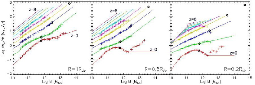
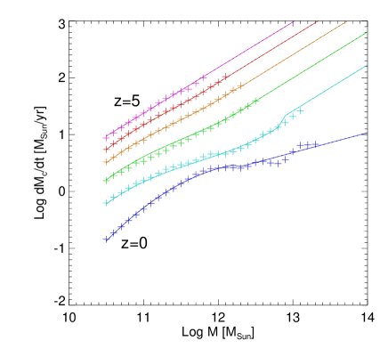
2) cold gas accretion rate $\dot{M}_{\rm c}$ . We use cold gas accretion rates from the simulation of FG11 without winds, primarily because these authors have provided $\dot{M}_{\rm c}$ at a few different radii inside a halo. This is important because $\dot{M}_{\rm c}$ are lower near the halo centres, especially at low redshifts. FG11 have provided median cold gas accretion rates in shells located at $0.2,0.5$ and $1\times R_{\rm vir}$ as a function of dark matter halo masses at redshifts $z=0,1,2,3,4,5$. These rates are computed directly using instantaneous velocity vectors of particles. They include both accretion through mergers and smooth accretion. Thicknesses of the shells are 0.2, 0.2, 0.1 $R_{\rm vir}$, respectively. We estimate $\dot{M_{c}}$ at all relevant masses and redshifts by interpolating and extrapolating $\dot{M_{c}}$ from FG11 (see Appendix §A.1). In Figure 1 we present $\dot{M_{\rm c}}$ at 1, 0.5, and 0.2 $R_{\rm vir}$, at different masses and redshifts.

3) $f_{\alpha}$ - fraction of energy that we see in Ly$\alpha$. Ly$\alpha$ flux is diminished by absorption through the intergalactic medium (IGM), particularly at the blue side of the line. We use effective optical depth of Faucher-Giguère et al. (2008) : $\tau_{\rm eff}=0.0018(1+z)^{3.92}$ (their eq. 21). We account for the IGM opacity by multiplying the calculated emissivities by $f_{\alpha}=0.5+0.5\exp(-\tau_{\rm eff})$ . Here, we assume that half of the Ly$\alpha$ flux is emitted from the blue side of the line, and that the whole flux from the red side of the line is transmitted. If LAB emission originates mainly from cold gas accretion, then dust opacity within the galaxy would be negligible.

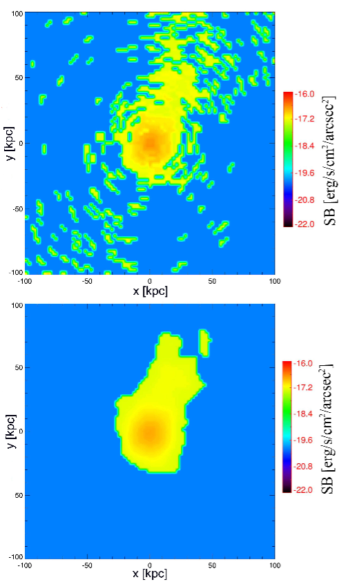
4) Cold gas filaments. In previous work it was shown that cold gas is placed along dark matter filaments inside a halo (see e.g. Dekel et al., 2009). Considering that we use pure DM simulation without gas, we further divide each shell into cells, and assume that within each shell cold gas is distributed uniformly and only in cells where dark matter density is larger than the halo’s average density in dark matter. A shell which is situated between spheres of radii $nL_{\rm soft}$ and $(n+1)L_{\rm soft}$, $n\geq 1$ is divided into $n+1$ parts, such that their projection onto xy-plane consists of $n+1$ concentric circles with radii $L_{\rm soft}\times j,j=1,2,...,n+1$. Then, each part whose projection is between circles of radii $jL_{\rm soft}$ and $(j+1)L_{\rm soft}$, $j\geq 1$, is further divided into $2j$ equal cells which enclose the same angles with the halo centre. In this way, the cells have roughly equal dimensions and their projection is straightforward to calculate. Then, SB maps are obtained by projecting haloes onto the xy-plane (see the upper image in Figure 2).

5) LABs images and influence of the atmosphere (seeing). The SB images are transferred into rectangular coordinate system with cells of size $L_{\rm soft}$, for all redshifts $z\gtrsim 2.3$. Then, at $z\gtrsim 2.3$ the images are smoothed with a 2D Gaussian kernel of FWHM which corresponds to the seeing of 1 arcsec, which is approximately equal to the seeing in LABs surveys. At $z\sim 1$ softening length in DM simulation is smaller than the 5.3 arcsec spatial resolution in the corresponding GALEX NUV band observations, thereby at $z\sim 1$ we merge a few cells in order to obtain similar resolution. Afterwards, in every halo we find all objects which do not contain adjacent cells with common vertices above a chosen SB threshold. At $z=1,2.3,3.1,4,5,6.6$ we use SB thresholds from the observations of Barger et al. (2012), Yang et al. (2009), Matsuda et al. (2004), Saito et al. (2006), and Ouchi et al. (2009). For every source we calculate its luminosity by summing the luminosities from all its cells above the SB threshold (hereafter these luminosities are denoted by $L_{\rm CR,obs}$, while cooling radiation luminosities from all cells are denoted by $L_{\rm CR,tot}$). Image of one of our LABs is presented in Figure 2. After smoothing, the emission is less fragmented and more similar to the observed LABs, while, on average, luminosities and areas are smaller.

4.2 Ly$\alpha$ from star formation

Newly formed stars could photoionize surrounding neutral HI gas and radiate in Ly$\alpha$. Luminosities in Ly$\alpha$ and H$\alpha$ trace star formation rate (SFR). H$\alpha$ emission originates mostly from HII regions around young hot stars. SFR is obtained when this emission is extrapolated to lower mass stars, by assuming Salpeter initial mass function. For case B recombination the relation between the emitted luminosity and SFR is derived from a combination of equation 2 in Kennicutt (1998) and of Brocklehurst (1971). The observed luminosity is calculated by multiplying the emitted luminosity by the escape fraction $f_{\rm esc}$, which denotes the fraction of the emitted luminosity which is not absorbed by the dust inside a halo or by IGM, and is observed from the Earth. The relation between the observed luminosity and SFR is:

$${L_{Ly\alpha}=1.1\times 10^{42}\times f_{\rm esc}{\rm SFR}.}$$ (4)

We calculate luminosities from SFR as follows:

1) Stellar mass. For each halo we calculate its stellar mass, using equations given in Behroozi et al. (2013). Behroozi et al. (2013) matched observed galaxies to their host haloes by using dark matter simulations and observed stellar mass function and star formation rates (SFR), and determined how stellar mass is related to halo mass and redshift. Their results are in agreement with observed stellar mass functions and SFRs at a range of redshifts $z=0-8$. We use their equations (3) and (4):

$$\log_{10}(M_{\ast}(M_{h})) = \log_{10}(\epsilon M_{1})+f\left(\log_{10}\left(\frac{M_{h}}{M_{1}}\right)\right)-f(0)$$

$$f(x) = -\log_{10}(10^{\alpha x}+1)+\delta\frac{(\log_{10}(1+\exp(x)))^{\gamma}}{1+\exp(10^{-x})}.$$ (6)

$$\nu(a) = \exp(-4a^{2})$$

$$\log_{10}(M_{1}) = M_{1,0}+(M_{1,a}(a-1)+M_{1,z}z)\nu$$

$$\log_{10}(\epsilon) = \epsilon_{0}+(\epsilon_{a}(a-1)+\epsilon_{z}z)\nu+\epsilon_{a,2}(a-1)$$

$$\alpha = \alpha_{0}+(\alpha_{a}(a-1))\nu$$

$$\delta = \delta_{0}+(\delta_{a}(a-1)+\delta_{z}z)\nu$$

$$\gamma = \gamma_{0}+(\gamma_{a}(a-1)+\gamma_{z}z)\nu.$$ (7)

Here $M_{\ast}$ is stellar mass, $M_{h}$ is halo mass, $z$ is redshift, $a$ is scale factor, and the rest are parameters. The parameters are taken from Behroozi et al. (2013).

2) Correcting stellar masses in merger trees. For some haloes, stellar mass is smaller than in the previous snapshot, and calculated SFR has a negative value. When two haloes are merging, some particles become gravitationally unbound, implying that the halo’s virial mass is smaller than in the previous snapshot. Then, in the following snapshot, merger remnant forms and new halo virializes. In some cases, this intermediate snapshot catches the moment of merger when material unbinds and halo’s mass decreases. We correct halo masses for this effect by interpolating between the snapshots, in those cases where the drop in halo mass occurs.

3) SFRs. For a halo $i$ with mass $M$ at redshift $z$ we calculate SFR in the following manner. We find all progenitors of halo $i$ in previous snapshot (at redshift $z+{\rm d}z$). Then we calculate stellar mass M_∗ of the halo $i$, and subtract stellar masses of progenitor haloes. This difference is the mass in stars which formed between two consecutive snapshots. Finally, we divide this mass with the time interval between $z$ and $z+{\rm d}z$:

$${SFR(i,z)=\frac{M_{*}(i,z)-\sum_{j=0}^{k}M_{*}(j,z+dz)}{dt}.}$$ (8)

In section §5.4 we show that our SFR functions at its bright end are in agreement with other recent works (e.g. Tescari et al., 2014).

4) Luminosities from SFRs. Ly$\alpha$ luminosities are calculated from eq. (4), where for $f_{\rm esc}$ we have used fit from Dijkstra & Jeeson-Daniel (2013), $f_{\rm esc}(z)=e^{-4.0+0.52z}$. Their $f_{\rm esc}$ includes IGM opacity. Dijkstra & Jeeson-Daniel (2013) determined $f_{\rm esc}$ by comparing observed SFR functions to Ly$\alpha$ luminosity functions from observations of LAEs at redshifts $z=0.35,3.1,3.7,5.7$. They successfully reproduced observed LAEs luminosity functions with $f_{\rm esc}$ which depends only on redshift, not on halo mass or SFR, over $\sim 2$ orders of magnitude in the luminosity. But, when we implemented the same $f_{\rm esc}$ in our model, LFs were not well reproduced at high redshifts, so we fitted ours (see Figure 5 and $f_{\rm esc1,2}$ in Figure 4).

4.3 Luminosity functions

Cumulative luminosity function (LF) displays the number density of objects with luminosities greater than $L$.

However, volumes with different density could have a range of different LFs. In order to account for this effect, we chose 1000 random cubical sub-volumes from the DM simulation box. Each sub-volume has a volume equal to an observing survey of LABs at the same redshift. At $z=0.8-1,1.5-2.3,3.1,4-5,6.6$ we chose surveys of Keel et al. (2009) (one half of their total volume, which would roughly correspond to the volume around one of the observed clusters), Erb et al. (2011) (which is almost the same as Yang et al. (2010) (CDFS)), Matsuda et al. (2004), Saito et al. (2006), and Ouchi et al. (2009), respectively.

For each LF we calculate (in log-scale) the area below it on the Figure 4. These areas we will call LF-areas. Then, we distribute all LF-areas into bins, fit a gaussian distribution, and find the mean value. We define the mean LF as the average of all LFs from the bin in which the mean LF-area is situated. LFs which differ by $\pm 2\sigma$ from the mean are determined from those two LF-areas which enclose $\pm 2\sigma$ values around the mean LF-area.

5 Results

5.1 Luminosity versus mass

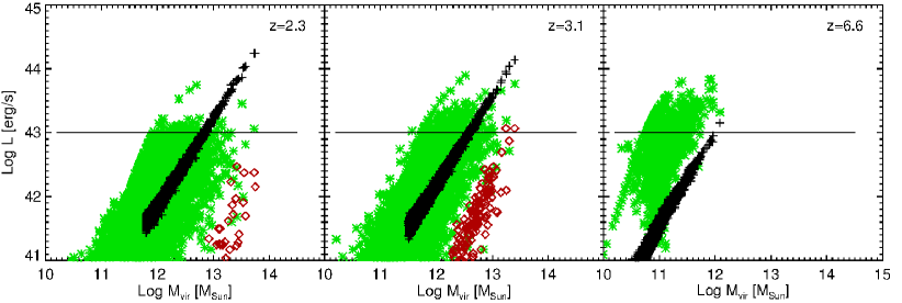
In Figure 3 we show how the modelled luminosities are related to halo masses. This includes SF luminosities ($L_{\rm SF}$); cooling radiation luminosities above a corresponding SB threshold - for the most luminous source inside a halo ($L_{\rm CR,obs}$; see §4.1); and total cooling radiation luminosities ($L_{\rm CR,tot}$), which includes total cooling radiation luminosity from all cells.

At $z\sim 3$ our relation halo mass - luminosity $L_{\rm CR,tot}$ is similar to the same relation in Dijkstra & Loeb (2009) model, and in Faucher-Giguère et al. (2010) prescription 7. However, in comparison to Rosdahl & Blaizot (2012), our relation halo mass - luminosity is steeper, and our luminosities are lower. The Figure also shows that $L_{\rm CR,obs}$ are less than $L_{\rm CR,tot}$ by $\sim$ an order of magnitude, or more. This difference is the most significant at lower redshifts, where haloes are more extended and have more rarefied gas, and at higher redshifts $z\gtrsim 5$, where the sources are less luminous.

Figure 3: Luminosity versus mass. Green stars represent luminosities from star formation, red diamonds are luminosities from cooling radiation above SB threshold, and black pluses are total luminosities from cooling radiation. Line at $L=10^{43}$ erg s^-1 represents a minimum luminosity above which could be detected LABs in most observations.

5.2 Luminosity functions from cooling radiation

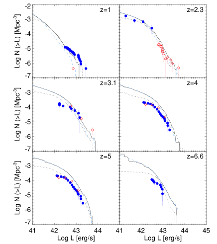
In Figure 4 we present cumulative luminosity functions at different redshifts calculated from:

1) our model with cooling radiation, $L_{\rm CR}$,

2) our model with star formation, $L_{\rm SF}$,

3) observations of LAEs and LABs in fields (symbols).

The Figure includes mean LFs and $\pm 2\sigma$ range from them, and Poisson errors for both observed and simulated data. The mean LFs almost coincide with the LFs calculated in the whole simulation box.

Figure 4: LAB and LAE cumulative luminosity functions at a few different redshifts. Light blue lines present LFs from cooling radiation (above SB threshold), black lines are LFs from SF, and green lines are LFs from SF but calculated for our $f_{\rm esc}$ ($f_{\rm esc}$ are also indicated on the Figure: $f_{\rm esc,1}$ are from Dijkstra & Jeeson-Daniel (2013), while $f_{\rm esc,2}$ are our best fit). For LFs from SF (cooling radiation) full lines (dot-dashed lines) represent LFs in the whole simulation box, thick full (dot-dashed) lines represent mean LFs, upper and lower dashed (double-dot-dashed) lines represent $2\sigma$ value distribution around the mean LFs (see §4.3), and upper and lower dotted lines represent Poisson errors in the simulated LFs. Observations are presented with different symbols: filled circles are observed LAEs LFs, while red symbols are observed LABs LFs. At $z=2.3$ different LABs observations are denoted with different symbols: diamonds are Yang et al. (2009) and triangles are Yang et al. (2010) (fields). Observations in fields ($\delta\sim 0$) at other redshifts are summarized in section 3. Observed LFs are presented with Poisson error bars.

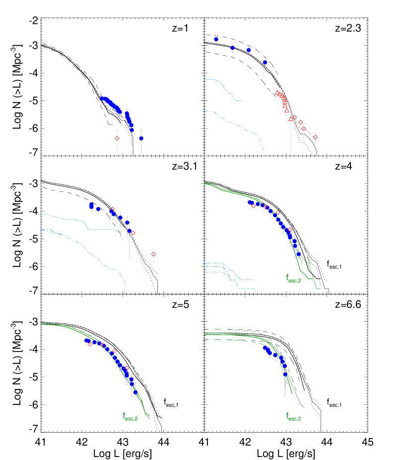
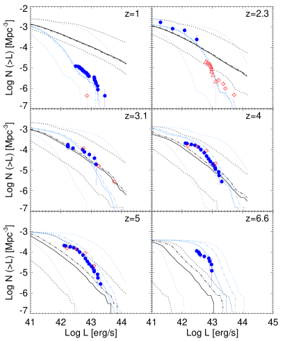
At all redshifts LFs calculated from cooling radiation are below the observed ones. This could be seen particularly at lower ($z\sim 1$) and at higher ($z\sim 6$) redshifts. At $z\sim 2-4$ our $L_{\rm CR}$ are too low to explain the observed LABs and LAEs LFs. At $z\sim 1$ and $z\gtrsim 5$ we did not obtain any Ly$\alpha$ emission from cooling radiation above the SB thresholds. Even if for every halo we sum luminosity from all cells above the SB threshold, our LFs would still be below the observed ones. Our results show that cooling radiation, as we modelled it, is insufficient to power most of LABs, at every redshift from $z=1-6.6$ and at every halo mass.

5.3 Luminosity functions from star formation

At a range of redshifts $z=1-5$ we obtain a good agreement of our LFs with observed LABs and LAEs LFs. At $z\sim 2.3-3.1$ observed LABs and LAEs LFs are falling inside $\pm 2\sigma$ from the mean modelled LFs, eventually with the exception of the most luminous LABs at $z\sim 3$. At $z=1$ our LF is in a good agreement with the observed LAEs LF, however somewhat above. This could be explained by additional AGN activity, as is detected in some of these LAEs. One LAB detected at $z=1$ is roughly falling inside $\pm 2\sigma$. At $z=4-5$ our LFs are in agreement with the observed LAEs and LABs LFs , however our values are somewhat above the observations.

At redshift $z=6.6$ our LF is above the observed LAEs LF, implying that our SF luminosities are too high. This could be explained if the most massive haloes are overabundant or have too high SFRs, or if $f_{\rm esc}$ is overestimated. Actually, massive haloes at high redshift are slightly overabundant (Martinović 2015), but we do not expect that this would significantly influence our results. On the other hand, our SFR functions (SFRFs) are in agreement with other work (see section §5.4), but note that at high luminosities observations are rare, and results from various models could differ. In comparison with Schechter SFRFs from Smit et al. (2012), which used Dijkstra & Jeeson-Daniel (2013), SFRs from our model are too high in massive haloes at high redshifts.

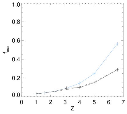
If the number density of massive haloes and SFRs are not overestimated significantly, than $f_{\rm esc}$ should be smaller. In Figure 4 we also show our LFs, but with $f_{\rm esc}$ for which we obtain the best agreement with observations (denoted by $f_{\rm esc,2}$). In this case, for appropriate $f_{\rm esc}$ we obtain a good agreement with the data. As a function of redshift, our $f_{\rm esc}$ could be fitted with a function of the same shape as in Dijkstra & Jeeson-Daniel (2013), $f_{\rm esc}(z)=e^{-a-bz}$, with parameters $a=3.76,b=-0.38$. At $z\geq 4$ we will further use our $f_{\rm esc}$.

In Figure 5 we show our escape fraction as a function of redshift. While at $z\lesssim 3$ our $f_{\rm esc}$ are almost the same as in Dijkstra & Jeeson-Daniel (2013), at higher redshifts the $f_{\rm esc}$ are smaller, but not ruled out from Dijkstra & Jeeson-Daniel (2013) with a great significance. For example, at $z\sim 4$ and $z\sim 6.6$ we found $f_{\rm esc}\sim 0.10$ and $f_{\rm esc}\sim 0.29$, respectively, while Dijkstra & Jeeson-Daniel (2013) fit gives $f_{\rm esc}\sim 0.15$ ($f_{\rm esc}\sim 0.1-0.2$) and $f_{\rm esc}\sim 0.57$ ($f_{\rm esc}\sim 0.35-0.92$) (see also discussion in Dijkstra & Jeeson-Daniel (2013)). In addition, note that differences between our model and Dijkstra & Jeeson-Daniel (2013) could influence the calculated $f_{\rm esc}$: our SFRFs differ from Schechter functions, we do not have scattering in $f_{\rm esc}$, we include observed LFs at redshifts higher than $z=5.7$, and we are not using non-cumulative luminosity functions.

Figure 5: Escape fraction as a function of redshift. Blue line is $f_{\rm esc}$ from Dijkstra & Jeeson-Daniel (2013). Full black line with symbols represents our $f_{\rm esc}$, and black dashed line represents fit to our $f_{\rm esc}$.

5.3.1 Influence of overdensity

Figure 6: LFs for SF model, as calculated in the most overdense regions, at redshifts $z=2.3$, 3.1, 6.6. Diamonds represent observations from Yang et al. (2010) (protocluster; $z=2.3$), Matsuda et al. (2004) ($z=3.1$) and Ouchi et al. (2009) ($z=6.6$); triangles represent observations from Erb et al. (2011) ($z=2.3$).

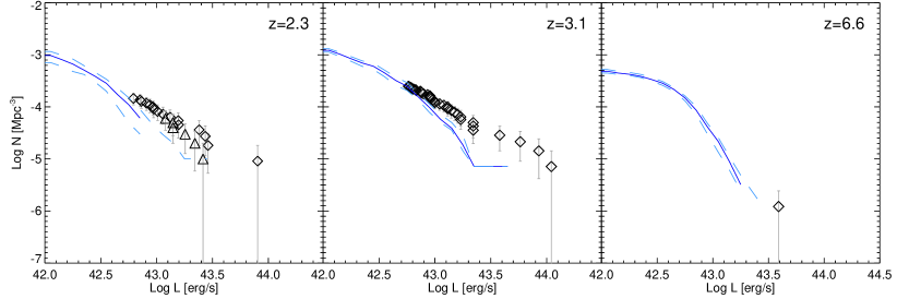
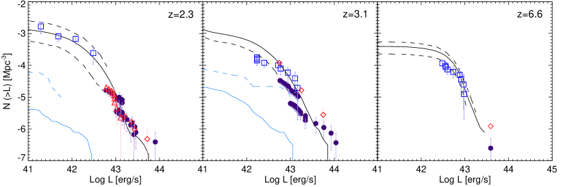
Figure 6 represents LFs in the most overdense regions at $z=2.3$, 3.1 and 6.6. We randomly choose 3000 sub-volumes with the same volume as in observations in overdense regions (Yang et al. (2010) at $z=2.3$, Matsuda et al. (2004) at $z=3.1$ and Ouchi et al. (2009) at $z=6.6$). We calculate LFs in the most overdense sub-volumes, with dark matter overdensity higher than $\delta_{\rm min}+(\delta_{\rm max}-\delta_{\rm min})\times 0.85$. Here, $\delta_{\rm min}$ and $\delta_{\rm max}$ are minimum and maximum density contrast of all sub-volumes. The Figure shows that the calculated LFs are roughly in agreement with observations, but somewhat lower at the highest luminosities ($\sim$ half order of magnitude at $z=3.1$). This could be explained if the most overdense sub-volumes are less dense than the observed protoclusters. The maximum density contrasts in dark matter and in the number of LAEs in subvolumes are equal to 0.6, 2, 1.8 , and to 0.5, 1.3, 1.4 at $z=6.6,3.1,2.3$, respectively.

5.4 SFR functions

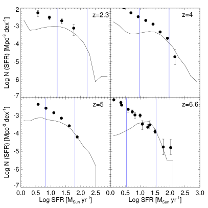
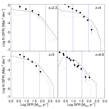
In order to investigate how accurate our method is, we compare our star formation rate functions (SFRFs) with other similar works at $z\sim 2-7$ (Figure 7). The Figure shows that for high SFRs, $\log SFR\gtrsim 1-1.5M_{\odot}$ yr^-1, our results are in agreement with observations (Hayes et al. (2010) at $z\sim 2.3$ and Smit et al. (2012) at $z\sim 4-6.6$). These SFRs correspond roughly to luminosities $\log L\gtrsim 42-43$.

However, in comparison with Schechter SFRFs from Smit et al. (2012) (which used Dijkstra & Jeeson-Daniel (2013); not shown in the Figure), SFRs from our model are higher in massive haloes at high redshifts. For example, at $z=4$ at $\log SFR\sim 2.3$ our SFRF gives $N=-4.8{\rm Mpc^{-3}dex^{-1}}$, while Smit et al. (2012) gives $N=-5.5{\rm Mpc^{-3}dex^{-1}}$. Similar conclusions hold at $z>4$. On the other hand, observations at bright end are rare, and results from various models could differ (see e.g. Tescari et al., 2014). Roughly, our SFRFs at bright end are in the range between different simulations of Tescari et al. (2014). We mention that, as Dijkstra & Jeeson-Daniel (2013) discussed, SFRFs are better described by Saunders functions instead of Schechter functions (Salim & Lee, 2012). These functions are almost identical at smaller luminosities, but at higher luminosities Saunders functions decrease more slowly, which is consistent with our larger number of more luminous haloes.

At small SFRs our SFRFs are too small, due to the limited resolution for the minimum halo mass $M_{\rm min}$ in DM simulation. We could apply our results at $\log SFR\gtrsim 1-1.5M_{\odot}$ yr^-1, which corresponds to luminosities $\log L\gtrsim 42-42.5$ erg s^-1. Influence of resolution is further discussed in Appendix §A.3.

Figure 7: Star formation rate functions from our model at redshifts $z\sim 2.3,4,5,6.6$. Blue vertical lines denote $\log SFR$ which correspond to luminosities $L=10^{42}$ and $10^{43}$ erg s^-1. Filled circles are the observations from Hayes et al. (2010) (at $z=2.3$) and from figure 2 in Smit et al. (2012) (at $z=4-6.6$). Smit et al. (2012) used results from UV observations in Bouwens et al. (2007, 2011).

5.5 Relation luminosity - stellar mass

Figure 8: Luminosity as a function of stellar mass, at redshifts $z=3.1$ (black diamonds) and at $z=6.6$ (light blue pluses).

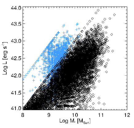
In Figure 8 we present luminosity ($L_{SF}$) as a function of stellar mass. As expected, haloes with larger masses and situated at higher redshifts show larger luminosities. Our results are roughly in agreement with LAB stellar masses estimated in different observations at $z\sim 3-6$. LAB stellar masses estimated in observations at $z\sim 3$ are $\sim 1-5\times 10^{11}M_{\odot}$ for LABs with luminosity $L\sim 10^{44}$ erg s^-1 (see Smith et al., 2008; Martin et al., 2014) , and at $z\sim 6.6$ for a LAB with luminosity $L\sim 4\times 10^{43}$ erg s^-1 the estimated stellar mass is $\sim 3.5\times 10^{10}M_{\odot}$ (see Ouchi et al., 2009).

6 Discussion

Sections §6.1, §6.2 and §6.3 discuss LAB areas, influence of the parametes used, and bias factor of LABs. Other uncertainties include assumption that particles inside a halo are spherically symmetrically distributed, lack of radiative transfer calculation (see e.g. Faucher-Giguère et al., 2010), and lack of influence of other sources of energy (such as AGN and starburst supernovae). LAB source of energy is discussed in section §6.4.

6.1 LAB areas in SF model

By using the method presented in §4.2, we could not calculate LAB areas. We estimate LABs areas by assuming how luminosity is distributed inside haloes.

In previous works the surface brightness profiles of extended Ly$\alpha$ emission are well fitted by

$${SB(r)=C\exp(-r/\beta),}$$ (9)

where $C$ and $\beta$ are free parameters, and $r$ is the projected radius (see Steidel et al., 2011; Momose et al., 2014; Matsuda et al., 2012). The parameters ranges are $C=1.4-15.7$ and $\beta=25.2-28.4$ in Steidel et al. (2011) for all objects except Ly$\alpha$ absorbers, and $C=0.8-5.3$ and $\beta=5.9-12.6\approx$ const in Momose et al. (2014) for LAEs at $z=2.2-6.6$.

Motivated by these results, we assume that in all haloes luminosity is distributed (spherically symmetrically) as in eq. (9), with a constant parameter $\beta$. For a few different $\beta$, for the calculated total luminosities we determine parameter $C$, and find the luminosities and areas above a surface brightness threshold which correspond to observations. In this simplified approach Ly$\alpha$ emission is described by no more than one component (for a more complex model see Wisotzki et al., 2015).

In Figure 9 we show LFs, cumulative area functions (AFs; defined in the same way as LFs) and the relation luminosity – area, calculated for a few different parameters $\beta$. The results are shown for observations of Yang et al. (2010) (fields) and Yang et al. (2009), at redshift $z=2.3$ and for surface brightness (SB) threshold $SB_{\rm thr}=5.5\times 10^{-18}$ erg s^-1 cm^-2 arcsec^-2. From the Figure 9 one can see that for $\beta\sim 5-10$ the calculated LFs, AFs and the relation between luminosities and areas are roughly in agreement with observations. The calculated LFs for $\beta\sim 5$ are almost the same as LFs for total luminosities. As $\beta$ increases, luminosities and areas are smaller, and areas increase faster with luminosities.

In Figure 10 we show the luminosity-area relation for a few different observations, at different redshifts. At $z\sim 2-3$ we obtain agreement with observations for $\beta\sim 5-10$. For LABs observed at $z=2.3$ by Erb et al. (2011) above a lower SB threshold, $SB_{\rm thr}=1.5\times 10^{-18}$ erg s^-1 cm^-2 arcsec^-2, we find $\beta\sim 15$. However, at $z=1$ and at $z=6.6$ we could obtain agreement with observations only if $\beta\sim 1.4$ and $\beta\gtrsim 42$, respectively. Our results at $z\sim 2.3$ are in agreement with Momose et al. (2014), who obtained $\beta\sim 5-10$ at $z=2.2-6.6$. However, our results are not in agreement with Steidel et al. (2011), who obtained $\beta=27.6$ for LABs. We speculate that this could be explained if the geometry of LABs influences significantly on the determined parameter $\beta$. It is observed that LABs have asymmetric shapes (see e.g. Matsuda et al., 2011). If stacked images of LABs have more shallow SB profiles and larger $\beta$, then LABs with asymmetric shapes could show larger luminosities and smaller areas (than in the case when they have symmetrical shapes), which apparently corresponds to lower $\beta$. On the other hand, luminosity – area relation for two LABs observed at $z=1$ and $z=6.6$ indicates that, assuming that the presented model well describes LABs, the parameter $\beta$ could increase with redshift, which is not in agreement with Momose et al. (2014).

Figure 9: LFs (left), AFs (central) and luminosity-area relation (right) calculated for SB distribution described with eq. (9). The results are shown for $z=2.3$ and SB threshold as in Yang et al. (2010). Different lines correspond to different parameter $\beta$, in the right (left and central) figure from bottom to upper (upper to botom): $\beta=$ 5,10,15,20,25,30. Black lines (denoted with $L_{\rm tot}$) correspond to total luminosities. Symbols represent different observations: diamonds represent results for fields in Yang et al. (2010), triangles are for Yang et al. (2009), and squares are for protocluster in Yang et al. (2010).

Figure 10: Luminosity-area relation calculated for a few different observations, from the upper left to the bottom right: Ouchi et al. (2009) ($z=6.6$), Matsuda et al. (2004) ($z=3.1$; triangles represent two LABs observed by Matsuda et al. 2009), Erb et al. (2011) ($z=2.3$), Barger et al. (2012) ($z=1$). Observations are represented by symbols. Different lines correspond to different parameter $\beta$, from bottom to upper: $\beta=$ 1.4,5,10,15,20,25,30,42 (at some $z$ only the lines for the lowest $\beta$ are shown).

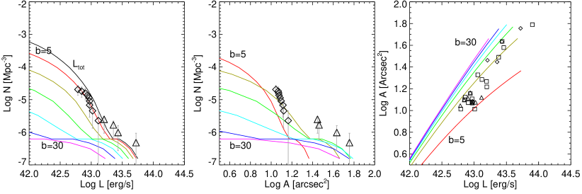
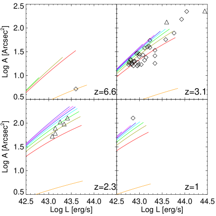
6.2 LFs for a range of parameters

In this section we present LFs at a few redshifts $z$, calculated for different parameters, from SF and from cooling radiation models.

Figure 11: LFs calculated from SF at a few different redshifts. The notation is the same as in the Figure 4, but the results are shown for different stellar masses (black thick lines are for Moster et al. (2013), and light blue lines are for Behroozi et al. (2013)) and for different escape fractions (full lines are for $f_{\rm esc}$ as calculated in Dijkstra & Jeeson-Daniel (2013), dot-dashed lines are for $f_{\rm esc}$ as calculated in our fit, dotted lines correspond to fixed $f_{\rm esc}=0.01$ and $f_{\rm esc}=1$).

Luminosities from star formation. Escape fractions and relation between stellar masses and dark matter masses are not well determined (see e.g. Kravtsov et al., 2014; Sawala et al., 2014; Dijkstra & Jeeson-Daniel, 2013). For example, Kravtsov et al. (2014) showed that at high masses Behroozi et al. (2013) underestimated stellar masses because they used observations which did not account for the outer SB profiles of their galaxies.

In Figure 11 we show LFs calculated from SF, but for different stellar masses (from Behroozi et al. (2013) and from Moster et al. (2013), their eq. (2),(11)-(14)) and escape fractions (as in Dijkstra & Jeeson-Daniel (2013), as in our fit, and for fixed values of 1 and 0.01). For stellar masses in Moster et al. (2013) we use their eq. (2) for both central and satellite galaxies (note that this could influence on the results to some extent). One can see that in order to obtain agreement of LFs calculated using stellar masses from Moster et al. (2013) with observations, the $f_{\rm esc}$ should be higher at luminosities $L\sim 10^{42}-10^{43}$ erg s^-1 at redshifts $z\gtrsim 4$, and at luminosities $L\gtrsim 10^{43}$ erg s^-1 and redshifts $z\lesssim 2.3$ it should be $f_{\rm esc}<0.01$.

Luminosities from cold gas accretion rates. We calculate luminosities and areas for the first 100 haloes (within the largest friends-of-friends masses), for different combinations of parameters:

1) $\dot{M_{\rm c}}$ as calculated in Faucher-Giguère et al. (2011) and in van de Voort et al. (2011) (see Appendix §A.2). In differrent work different cold gas accretion rates ($\dot{M_{\rm c}}$) are obtained (see e.g. Faucher-Giguère et al., 2011, 2010; van de Voort et al., 2011; Rosdahl & Blaizot, 2012; Nelson et al., 2013; Benson & Bower, 2011). For example, at $z\sim 3$ at $\log M=12-12.5M_{\odot}$ cold gas accretion rates in van de Voort et al. (2011) are by about order of magnitude higher than in FG11. On the other hand, Nelson et al. (2013) obtained smaller cold gas accretion rates onto massive galaxies at $z=2$ by a factor of up to two or more (see their fig. 3).

2) different slope of the extrapolation of the $\dot{M_{\rm c}}$ at high masses ($\pm 0.1\times(\log M-12)$)

3) different distribution of the $\dot{M_{\rm c}}$ at a fixed radius $r$: $f=1-20$, $g=0-10$. Simulations showed that cold gas is distributed along filaments of dark matter, where density is a few times higher than the average density inside a halo (see Dekel et al., 2009). We assume that the filaments are found in cells where the density is at least $f$ times higher at the virial radius, at least $g$ times higher at the halo center, and at radius $r$ at least $f+(g-f)\times(1-r/R_{\rm vir})$ higher; and we assume that cold gas is homogeneously distributed at each $r$.

Figure 12: LFs (left), AFs (central) and luminosity-area relation (right) calculated for cooling radiation model. The results are shown for $z=2.3$ and SB threshold as in Yang et al. (2010). For LFs and AFs thick black and light blue lines represent results for $\dot{M_{\rm c}}$ as calculated in Faucher-Giguère et al. (2011) and in van de Voort et al. (2011), respectively. Full and dashed lines represent lower and higher slopes of the extrapolation of the $\dot{M_{\rm c}}$ at high masses, respectively. For the luminosity-area relation, light blue crosses represent the results calculated for all these cases. Symbols represent observations of LAEs (blue circles), LABs in Yang et al. (2009) (diamonds) and LABs in Yang et al. (2010) (fields; triangles).

Figure 13: The same as in the Figure 12, but for luminosities of Saito et al. (2006) at $z\sim 3-5$.

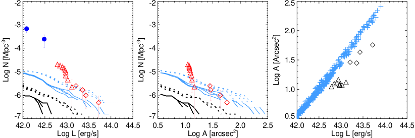
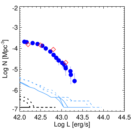
From Figure 12 one can see that using $\dot{M_{\rm c}}$ as calculated in Faucher-Giguère et al. (2011) LFs and AFs are below the observations. However, by using $\dot{M_{\rm c}}$ as calculated in van de Voort et al. (2011), one can obtain agreement with observed LFs or AFs at $z=2.3$ for appropriate parameters, but the luminosity – area relation is above the observations. On the other hand, Figure 13 shows that at $z\sim 4$ the LFs are below the observations in all cases.

6.3 Overdense regions and fields

Observations showed that in overdense regions, usually traced by LAE number counts, the number density of LABs is also higher (e.g. Yang et al., 2010). This implies that LAB cumulative luminosity functions (LFs) and number densities from different observations could not be directly compared, if the observed volumes have different densities. However, LABs are rare and are in many cases detected in protoclusters with different densities.

In this section it is described how the observed number densities of LABs from protoclusters with diverse matter densities could be compared to LABs detected in fields. In this way, for each observation of LABs it could be predicted what number of LAB would be detected in a volume of the same dimensions, but with average density (i.e. in the field). In this manner, LABs LFs could be compared between a few different surveys, and it could be roughly estimated how LAB number density (or LF) changes with redshift. For the discussion on influence of overdensity on calculated LAB LFs see also Yang et al. (2010) and appendix in Dijkstra & Loeb (2009); and for estimates of evolution of LAB number density with redshift see e.g. Keel et al. (2009).

Density contrast of LABs in some specific volume is defined as $\delta_{\rm LAB}=\frac{n_{\rm LAB}-\bar{n}_{\rm LAB}}{\bar{n}_{\rm LAB}}$, where $n_{\rm LAB}$ is the number density of LABs in the volume, and $\bar{n}_{\rm LAB}$ is the mean number density of LABs. Bias defines how the number density of some objects traces the distribution of the matter density. Bias of LABs ($b_{\rm LAB}$) is defined as

$${\delta_{\rm LAB}=b_{\rm LAB}\delta_{\rm m},}$$ (10)

where $\delta_{\rm LAB}$ is the density contrast of LABs, and $\delta_{\rm m}$ is the matter density contrast. Density contrast and bias of LAEs ($\delta_{\rm LAE}$ and $b_{\rm LAE}$) are defined in the same way.

We use the relative bias parameter between LABs and LAEs, $b_{1}$, which is defined as:

$${b_{1}=\frac{\delta_{\rm LAB}}{\delta_{\rm LAE}}=\frac{b_{\rm LAB}}{b_{\rm LAE}}.}$$ (11)

Equations (10) and (11) show that, if in a volume (protocluster) observed at redshift $z$ the number density of LABs is $n_{\rm LAB}$ and the LAEs density contrast is $\delta_{\rm LAE}$, then the number density of LABs in an average volume at $z$ is

$${\bar{n}_{\rm LAB}=n_{\rm LAB}/(b_{1}\delta_{\rm LAE}+1).}$$ (12)

For the most luminous LABs we derive $b_{1}$ using values of bias factor of LABs ($b_{\rm LAB}$) and LAEs ($b_{\rm LAE}$) which are calculated from observations. Yang et al. (2010) have determined bias factor for 6 most luminous and largest LABs discovered in their survey at $z=2.3$ (with $L\gtrsim 1.5\times 10^{43}$ erg s^-1, $A>16{\rm arcsec^{2}}$). They found that $b_{\rm LAB}\sim 7$. Guaita et al. (2010) have determined bias factor for LAEs at $z\sim 2.1\approx 2.3$, and found that $b_{\rm LAE}\sim 1.8$ (for other references see also Ouchi et al., 2010). From eq. (12), $b_{\rm LAB}$ and $b_{\rm LAE}$ we obtain

$${b_{1}\sim 3.9,}$$ (13)

Now we roughly estimate bias for less luminous and less large LABs in Yang et al. (2010) survey, with $L<10^{43}$ erg s^-1 and $A<16{\rm arcsec^{2}}$. We denote this bias factor by $b_{2}$, and mention that it is defined in the same way as $b_{1}$. First, we estimate variance using standard equation (Peebles 1980, §36):

$${\sigma_{v}^{2}=\frac{\langle N^{2}\rangle-{\langle N\rangle}^{2}}{{\langle N\rangle}^{2}}-\frac{1}{\langle N\rangle},}$$ (14)

and apply it to 4 fields which Yang et al. (2010) observed. This equation was also used by Yang et al. (2010), but for the most luminous LABs. We derive the bias factor for these less luminous LABs in the same way as for the most luminous LABs, and obtain

$${b_{2}=1.4,}$$ (15)

We will proceed further with the assumption that the the relative bias parameter between LABs and LAEs is constant with redshift and that for luminosities $L\gtrsim 1\times 10^{3}$ erg s^-1 it is equal to $b_{1}=3.9$, while for luminosities $L\lesssim 1.5\times 10^{3}$ erg s^-1 it is $b_{2}=1.4$.

Figure 14 represents LFs at $z=2.3$, 3.1 and 6.6, but which also include LFs from observations in the most overdense regions which are corrected for density contrast by using eq. 12. The Figure shows that the corrected LFs in overdensities are in agreement with observed LFs from fields. These LFs are also in agreement with LFs from our SF model.

Figure 14: LAB and LAE cumulative luminosity functions at $z=2.3$, 3.1 and 6.6. Light blue lines present LFs from cooling radiation, while black lines are LFs from SF. Dashed lines represent $2\sigma$ value distribution around the mean LFs. Symbols represent observed LAB and LAE LFs. Observed LAE LFs are represented with blue empty squares, and observed LAB LFs in fields at $z\sim 2-3$ are represented with red empty triangles and diamonds. Observations in overdensities are represented with filled violet circles, and include: Yang et al. (2010) (protocluster; $z=2.3$), Matsuda et al. (2004) ($z=3.1$), Erb et al. (2011) ($z=2.3$) and Ouchi et al. (2009) ($z=6.6$). For comparison, red empty diamond at $z=6.6$ represents data uncorrected for overdensity for Ouchi et al. (2009) LAB.

6.4 LAB source of energy

For appropriate $f_{\rm esc}$ our LAB and LAE LFs for SF model are in agreement with observations at $z\sim 1-6.6$, which is consistent with work in which SF might be the dominant source of energy in majority of LABs (e.g. Cen & Zheng, 2013; Colbert et al., 2011; Steidel et al., 2011). However, there is also evidence that SF and AGN could be insufficient to explain luminosities in some LABs (e.g. Nilsson et al. 2006, but see also Prescott et al. 2015). If this is true, this might indicate that we underestimated cooling radiation luminosities in some cases. If we would take into account duty cycle and variations of cold gas accretion rate in different haloes, then it could be possible to obtain larger cooling radiation luminosities in some, but not the majority, of the haloes. In addition, physics of cooling radiation is still not well understood (see discussion in Faucher-Giguère et al. 2010). For example, it is not well explored if the infalling streams of the cold gas maintain constant velocity and continuously radiate their gravitational energy, or if the streams freely fall into the haloes and release their energy only when they encounter the central galaxy through a shock. Also, for different cold gas accretion rates our results could change.

As is found in some observations, LABs could be complex phenomena which contain multiple galaxies and fragments of gas, which are powered by multiple sources of energy with different contribution in diverse LABs (e.g. Colbert et al., 2008; Prescott et al., 2012b; Colbert et al., 2011; Francis et al., 2012; Martin et al., 2014). It is also expected that different sources of energy are related to each other and that photoionization models require cold spatially extended gas in LABs’ host haloes (see e.g. discussion in Dijkstra & Loeb 2009).

7 Conclusions

In this work we have modelled LAB emission from cooling radiation from the intergalactic gas accreting onto galaxies and from star formation (SF). We have used a dark matter (DM) simulation, to which we applied semi-analytic recipes. These recipes include cold gas accretion rates from a hydrodynamical simulation, stellar masses from matching of DM haloes to observed galaxies, escape fraction of Ly$\alpha$ photons from comparison of observed SFR functions to Ly$\alpha$ luminosity functions, and intergalactic opacity from observations of Ly$\alpha$ forest. The advantage of our model is that we have a large volume and massive haloes at the same time.

Here we summarize our main conclusions:

1) We found that luminosities from cooling radiation are too small to explain observed LAB LFs, if we use cold gas accretion rates ($\dot{M}_{\rm c}$) from Faucher-Giguère et al. (2011). However, if we use $\dot{M}_{\rm c}$ from van de Voort et al. (2011), then our cumulative luminosity functions (LFs) are in agreement with observations at $z\sim 2.3$ for the most luminous LABs ($L>10^{43}$ erg s^-1), but at $z\sim 4$ our luminosities are still below observations. Our cooling radiation luminosities are almost independent on uncertainties in cold gas distribution, but to some extent depend on the extrapolation slope in $\dot{M}_{\rm c}$.

2) If we use escape fraction ($f_{\rm esc}$) from Dijkstra & Jeeson-Daniel (2013), then our LFs from SF model are in agreement with observed LABs and LAEs LFs, but only at $z\sim 1-3$. However, when we used our $f_{\rm esc}$, that is $f_{\rm esc}(z)$ of the same shape as in Dijkstra & Jeeson-Daniel (2013) but for which we found the best fitting parameters, then we found that our modelled LFs are in agreement with all observations of LAEs and LABs in fields at $z\sim 1-6.6$. For LABs in protoclusters our results are also in agreement with observations, but at high luminosities observed LABs might be somewhat more luminous. We note that our results might be dependent on the stellar masses used, and that they are in agreement for Behroozi et al. (2013) stellar masses used.

3) For SF model, we could reproduce luminosity – area relation of LABs at $z\sim 2-3$ for assumed exponential distribution of light inside haloes (eq. (9)), with a slope parameter $\beta\sim 5-10$. On the other hand, LAB areas at $z\sim 1$ and at $z\sim 6.6$ could be explained if parameter $\beta$ has lower or higher value than at $z\sim 2-3$.

4) Our results indicate that majority of LABs and LAEs at a range of redshifts $z\sim 1-6.6$ might be powered mainly by SF. However, we note that there exist other uncertainties in model, and that our results are dependent on parameters used.

Acknowledgements This work was supported by the Ministry of Education, Science and Technological Development of the Republic of Serbia through project no. 176001 “Astrophysical spectroscopy of extragalactic objects” and project no. 176021 “Visible and Invisible Matter in Nearby Galaxies: Theory and Observations”. We thank referee whose comments significantly improved the content of this paper, Milan Bogosavljević for initial idea and useful consultation during the work, Anne Verhamme for helpful comments on the manuscript. We also thank Masami Ouchi for helpful comments and discussion, and Mark Dijkstra, Luka Popović and Dušan Kereš for useful discussion. Numerical results for the DM simulation were obtained on PARADOX cluster at the Scientific Computing Laboratory of the Institute of Physics Belgrade, supported in part by the national research project ON171017, funded by the Serbian Ministry of Education, Science and Technological Development. The Millennium-II Simulation databases used in this paper and the web application providing online access to them were constructed as part of the activities of the German Astrophysical Virtual Observatory (GAVO).

Appendix A Appendix

A.1 Fit for cold gas accretion rates

In order to estimate $\dot{M_{\rm c}}$ at a given radius $r$ inside a halo ($r=1,0.5,0.2$ $R_{\rm vir}$), as a function of halo mass and redshift, we interpolate and extrapolate FG11 values for a few groups of ranges of halo masses and redshifts (Table 4). Between these radii we linearly interpolate $\dot{M_{\rm c}}$. At high masses, we ignore an increase of $\dot{M_{\rm c}}$ at $z=0$ for $r=0.5$ and 0.2 $R_{\rm vir}$ and a decrease of $\dot{M_{\rm c}}$ at $r=0.2R_{\rm vir}$ in FG11 , since there is a relatively small number of the most massive haloes. From Figure 1 we see that this fit well describes the $\dot{M}_{\rm c}$ from Faucher-Giguère et al. (2011).

Figure 15: Cold gas accretion rates at $R_{\rm vir}$, as calculated in van de Voort et al. (2011) (full lines) and our approximation (dashed lines). The results are shown at redshifts $z\sim 0,1,2,3,4,5$, from the lowest to the highest line (dark blue, light blue, green, orange, red, rose, respectively).

Table 4: Our interpolation and extrapolation of FG11 cold gas accretion rates at 1, 0.5 and 0.2 $R_{\rm vir}$ and at $z\geq 1$. Given are the radius, redshift range, mass range, and the used shape of a polynomial (as a function of $z^{\prime}=\log(1+z)$ and $M^{\prime}=\log M$). Here $M_{\rm lim,1}=13.1-0.3z$ and $M_{\rm lim,2}=12.4-0.2z$. Polynomials represent $\log\dot{M_{\rm c}}$.

radius $[R_{\rm vir}]$	$z$ range	$\log M$ range	polynomial $p(z^{\prime},M^{\prime})$
1	$1-5$	$>M_{\rm lim,1}$	$p(M^{\prime},z^{\prime})=a_{0}+a_{1}z^{\prime}+0.81M^{\prime}$ ∗1
1	$1-5$	$<M_{\rm lim,1}$	$p(M^{\prime},M^{\prime 2},M^{\prime 3},z^{\prime}M^{\prime},z^{\prime}M^{\prime 2},z^{\prime}M^{\prime 3})$
1	$>5$	$10-15$	$p(M^{\prime},z^{\prime},z^{\prime}M^{\prime})$
0.5	$1-5$	$>M_{\rm lim,2}$	$p(M^{\prime},z^{\prime})=a_{0}+a_{1}z^{\prime}+0.81M^{\prime}$
0.5	$1-5$	$<M_{\rm lim,2}$	$p(M^{\prime},M^{\prime 2},M^{\prime 3},z^{\prime}M^{\prime},z^{\prime}M^{\prime 2},z^{\prime}M^{\prime 3})$
0.5	$>5$	$10-15$	$p(M^{\prime},z^{\prime},z^{\prime}M^{\prime})$
0.2	$1,2,3,4$	$<11$	$p(M^{\prime})$
0.2	$1,2,3,4$	$>11$	$p(M^{\prime})$
0.2	$5$	$<11.2$	$p(M^{\prime})$
0.2	$5$	$>11.2$	$p(M^{\prime})$
0.2	$1-5$	$10-15$	lin. int. between 2 nearest integer redshifts
0.2	$>5$	$10-15$	lin. extrapolation from $z=4$ and $z=5$

^∗1 - coefficient 0.81 is used from Faucher-Giguère et al. (2011) fit for cold gas + interstellar medium accretion rates at $z\geq 2$. For $M>M_{\rm lim}$ at redshifts $z=1-5$ and at radii $R_{\rm vir}$ and $0.5R_{\rm vir}$ we use fit that has the same slope as that one of FG11. For each redshift ($z=1,2,3,4,5$) we find the point from the plot in the middle between the two points that are related to the most massive haloes: $\log M=\frac{1}{2}(\log M(1)+\log M(2))$, $\log\dot{M}_{c}=\frac{1}{2}(\log\dot{M}_{\rm c}(1)+\log\dot{M}_{\rm c}(2))$, and fit these 6 points with straight lines with shape $p(M^{\prime},z^{\prime})=a_{0}+a_{1}z^{\prime}+0.81M^{\prime}$.

^∗2 - linear interpolation

A.2 Cold gas accretion rates in van de Voort et al. (2011)

We approximate cold gas accretion rates calculated in van de Voort et al. (2011), $\dot{M}_{\rm c,vdv}$, as a function of cold gas accretion rates calculated in Faucher-Giguère et al. (2011), $\dot{M}_{\rm c,fg}$, as follows: for masses $M>M_{\rm lim,3}$: $\log\dot{M}_{\rm c,vdv}=\log\dot{M}_{\rm c,fg}+0.33$, and for masses $M<M_{\rm lim,3}$: $\log\dot{M}_{\rm c,vdv}=\log\dot{M}_{\rm c,fg}+(-4.83+0.42\log M+0.41\log(1+z))$, where $\log M_{\rm lim,3}=12.5-0.3z$ for $0.5<z<4$, $\log M_{\rm lim,3}=12.2$ for $z<0.5$, and $\log M_{\rm lim,3}=11.5$ for $z>4$.

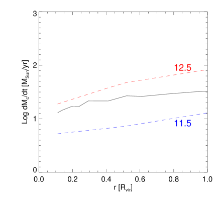
Figure 15 shows that in this way we could well describe $\dot{M}_{\rm c,vdv}$. We assume that the same relation between $\dot{M}_{\rm c,vdv}$ and $\dot{M}_{\rm c,fg}$ holds at each radius $r$ inside a halo. In Figure 16 we show that at $z=2$ and for halo masses $10^{11.5}M_{\odot}<M_{\rm halo}<10^{12.5}M_{\odot}$ our approximation of $\dot{M}_{\rm c,vdv}$ is in agreement with van de Voort et al. (2012) cold gas accretion rates at radii $r\sim 0.1-1R_{\rm vir}$ inside a halo.

Figure 16: Cold gas accretion rates as a function of radius inside haloes at $z=2$ and $10^{11.5}M_{\odot}<M_{\rm halo}<10^{12.5}M_{\odot}$ as calculated in van de Voort et al. (2012) (full line), their fig. 3. Dashed blue and red line denote our approximation at masses $10^{11.5}M_{\odot}$ and $10^{12.5}M_{\odot}$, respectively.

A.3 Resolution of the DM simulation

As Figure 7 shows the discrepancy at $SFR=10M_{\odot}$ yr^-1, we compare our results from the DM simulation with the results calculated from the Millennium-II simulation (Lemson et al., 2006; Boylan-Kolchin et al., 2009), which has more than 100 times better mass resolution and $2-3$ times smaller volume. Millennium-II simulation is a pure dark matter simulation, which is run in a periodic box of size $100$ Mpc $h^{-1}$, using cosmological parameters $(\Omega_{m},\Omega_{\Lambda},h)=(0.25,0.75,0.73)$. It uses $10^{10}$ particles with masses $6.9\times 10^{6}h^{-1}M_{\odot}$.

Figure 17: Star formation rate functions from our model at redshifts $z\sim 2.3,4,5,6.6$ (dotted lines) and from Millennium-II simulation. SFRFs are calculated from the Millennium-II simulation for total subhalo masses (light blue dashed lines) and for subhalo masses m-crit200 (black full lines; see the text). Other notation is the same as in the Figure 7.

Figure 18: Cumulative luminosity functions at a range of redshifts. Notations are the same as in the Figure 4, except that now full and dashed lines represent LFs calculated from the Millennium-II simulation, and dotted lines are LFs from DM simulation. Full and dashed lines represent LFs calculated for subhalo masses m-crit200 and for total subhalo masses, respectively.

Figure 19: Convergence properties of LFs and SFRFs. Maximum and minimum differences of LFs (full lines) and SFRFs (dashed lines) between the values calculated for minimum halo masses of $M_{\rm min}$ and $\sim 10^{10}M_{\odot}$, as a function of $M_{\rm min}$. Minimum differences are equal to $\sim 0$ for both LFs and SFRFs.

At each redshift, we select subhaloes with more than 1000 particles (which corresponds to a mass of $9.45\times 10^{9}M_{\odot}$). For each subhalo we select all of its progenitors from the previous snapshot with more than 50 particles. For all subhaloes we select its total mass. For subhaloes which are dominant in its friend-of-friends group, we select its mass m-crit200, which is the mass within the radius where the subhalo has an overdensity 200 times the critical density of the simulation.

Using these data, we calculate LFs and SFRFs in the same way as for DM simulation (Figures 17 and 18, respectively). When we use the Millennium-II simulation, the results are almost the same, except that at low end SFRFs are higher and in a relatively good agreement with observations. LFs almost did not change at the range of luminosities in which LABs and LAEs from Figure 4 are observed.

Figure 19 shows the convergence properties of LFs (for luminosities in the range $[10^{41},10^{44}]$ erg s^-1) and SFRFs (for SFRs in the range $[1,1000]$ $M_{\odot}$ yr^-1). It could be seen that for mass resolutions $M_{\rm min}\sim 10^{10.4}M_{\odot}$ and $M_{\rm min}\sim 10^{10}M_{\odot}$ the calculated LFs and SFRFs almost do not differ. Next, we examine convergence properties as following. We define an array with minimum halo masses $r=\log M_{\rm min}=[10.6,10.4,10.2,10]$, and an array of differences between a value of a LF(L,z) calculated for $r_{i}$ and $r_{i+1}$: $b_{i}=LF(L,z,r_{i+1})-LF(L,z,r_{i})$. For the array $b$ it holds $0<b_{i}<0.15^{i}$, for $i=$ 0, 1, 2. If the same inequality holds for $i\geq 3$, then $LF(L,z,r_{i})<LF(L,z,r_{2})+0.15^{3}+...+0.15^{i}$. This implies that $LF(L,z,r_{i})$ and $LF(L,z,r_{2})$ would not differ by more than $0.15^{3}+...+0.15^{i}=(0.15^{3}-0.15^{i+1})/0.85$, which is less than 0.01. The same holds for SFRF(SFR,z).

References

- Barger et al. (2012) Barger A. J., Cowie L. L., Wold I. G. B., 2012, ApJ, 749, 106
- Basu-Zych & Scharf (2004) Basu-Zych A., Scharf C., 2004, ApJ, 615, L85
- Behroozi et al. (2013) Behroozi P. S., Wechsler R. H., Conroy C., 2013, ApJ, 770, 57
- Benson & Bower (2011) Benson A. J., Bower R., 2011, MNRAS, 410, 2653
- Binney & Tremaine (1994) Binney J., Tremaine S., 1994, Galactic Dynamics. Princeton Univ. Press, Princeton, NJ
- Bouwens et al. (2011) Bouwens R. J. et al., 2011, ApJ, 737, 90
- Bouwens et al. (2007) Bouwens R. J., Illingworth G. D., Franx M., Ford H., 2007, ApJ, 670, 928
- Boylan-Kolchin et al. (2009) Boylan-Kolchin M., Springel V., White S. D. M., Jenkins A., Lemson G., 2009, MNRAS, 398, 1150
- Bridge et al. (2012) Bridge C. R. et al., 2012, preprint (arxiv:1205.4030)
- Brocklehurst (1971) Brocklehurst M., 1971, MNRAS, 153, 471
- Cen & Zheng (2013) Cen R., Zheng Z., 2013, ApJ, 775, 112
- Chapman et al. (2001) Chapman S. C., Lewis G. F., Scott D., Richards E., Borys C., Steidel C. C., Adelberger K. L., Shapley A. E., 2001, ApJ, 548, L17
- Coil (2013) Coil A. L., 2013, The Large-Scale Structure of the Universe, Springer
- Colbert et al. (2011) Colbert J. W., Scarlata C., Teplitz H., Francis P., Palunas P., Williger G. M., Woodgate B., 2011, ApJ, 728, 59
- Colbert et al. (2008) Colbert J. W., Teplitz H., Francis P., Palunas P., Williger G. M., Woodgate B., 2008, ASPC, 381, 468
- Crocce et al. (2006) Crocce M., Pueblas S., Scoccimarro R., 2006, MNRAS, 373, 369
- Davis et al. (1985) Davis M., Efstathiou G., Frenk C. S., White S. D. M., 1985, ApJ, 292, 371
- Dawson et al. (2007) Dawson S., Rhoads J. E., Malhotra S., Stern D., Wang J., Dey A., Spinrad H., Jannuzi B. T., 2007, ApJ, 671, 1227
- Dekel & Birnboim (2008) Dekel A., Birnboim Y., 2008, MNRAS, 383, 119
- Dekel & Birnboim (2006) Dekel A., Birnboim Y., 2006, MNRAS, 368, 2
- Dekel et al. (2009) Dekel A. et al., 2009, Nature, 457, 451
- Dijkstra & Jeeson-Daniel (2013) Dijkstra M., Jeeson-Daniel A., 2013, MNRAS, 435, 3333
- Dijkstra & Loeb (2009) Dijkstra M., Loeb A., 2009, MNRAS, 400, 1109
- Erb et al. (2011) Erb D. K., Bogosavljević M., Steidel C. C., 2011, ApJL, 740, L31
- Faucher-Giguère et al. (2011) Faucher-Giguère C.-A., Kereš D., Ma C.-P., 2011, MNRAS, 417, 2982
- Faucher-Giguère et al. (2010) Faucher-Giguère C.-A., Kereš D., Dijkstra M., Hernquist L., Zaldarriaga M., 2010, ApJ, 725, 633
- Faucher-Giguère et al. (2008) Faucher-Giguèere C.-A., Prochaska J. X., Lidz A., Hernquist L., Zaldarriaga M., 2008, ApJ, 681, 831
- Finkelstein et al. (2007) Finkelstein S. L., Rhoads J. E., Malhotra S., Pirzkal N., Wang J., 2007, ApJ, 660, 1023
- Francis et al. (2012) Francis P. J., Dopita M. A., Colbert J. W., Palunas P., Scarlata C., Teplitz H., Williger G. M., Woodgate B. E., 2013, MNRAS, 428, 28
- Furlanetto et al. (2005) Furlanetto S. R., Schaye J., Springel V., Hernquist L., 2005, ApJ, 622, 7
- Gawiser et al. (2006) Gawiser E. et al., 2006, ApJ, 642, L13
- Geach et al. (2009) Geach J. E. et al., 2009, ApJ, 700, 1
- Geach et al. (2007) Geach J. E., Smail I., Chapman S. C., Alexander D. M., Blain A. W., Stott J. P., Ivison R. J., 2007, ApJ, 655, L9
- Geach et al. (2005) Geach J. E. et al., 2005, MNRAS, 363, 1398
- Goerdt et al. (2010) Goerdt T., Dekel A., Sternberg A., Ceverino D., Teyssier R., Primack J. R., 2010, MNRAS, 407, 613
- Guaita et al. (2010) Guaita L. et al., 2010, ApJ, 714, 255
- Haiman et al. (2000) Haiman Z., Spaans M., Quataert E., 2000, ApJ, 537, L5
- Hayes et al. (2013) Hayes M. et al., 2013, ApJL, 765, L27
- Hayes et al. (2011) Hayes M., Scarlata C., Siana B., 2011, Nature 476, 304
- Hayes et al. (2011b) Hayes M., Schaerer M., stlin G., Mas-Hesse J. M., Atek H., Kunth D., 2011, ApJ, 730, 8
- Hayes et al. (2010) Hayes M. et al., 2010, Nature, 464, 562
- Katz et al. (2003) Katz N., Kereš D., Dave R., Weinberg D. H., 2003, in Rosenberg J. L., Putman M. E., eds, The IGM/Galaxy Connection. The Distribution of Baryons at Vol. 281 of Astrophysics and Space Science Library, How Do Galaxies Get Their Gas?. p. 185
- Keel et al. (2005) Keel W. C., 2005, ApJ, 129, 1863
- Keel et al. (2009) Keel W. C., White III R. E., Chapman S., Windhorst R. A., 2009, ApJ, 138, 986
- Kennicutt (1998) Kennicutt Robert C. Jr., 1998, ARA&A, 36, 189K
- Kereš et al. (2009) Kereš D., Katz N., Fardal M., Davé R., Weinberg D. H., 2009, MNRAS, 395, 160
- Kereš et al. (2005) Kereš D., Katz N., Weinberg D H., Davé R., 2005, MNRAS, 363, 2
- Kravtsov et al. (2014) Kravtsov A., Vikhlinin A., Meshscheryakov A., 2014, preprint (arXiv: 1401.7329)
- Kudritzki et al. (2000) Kudritzki R.-P. et al., 2000, ApJ, 536, 19
- Lai et al. (2008) Lai K. et al., 2008, ApJ, 674, 70L
- Lemson et al. (2006) Lemson G. & the Virgo Consortium, 2006, arXiv:astro-ph/0608019
- Martin et al. (2014) Martin D. C., Chang D., Matuszewski M., Morrissey P., Rahman S., Moore A., Steidel C. C., Matsuda Y., 2014, ApJ, 786, 107
- Martinović (2015) Martinović N., 2015, Serb. Astron. J., 190, 11
- Matsuda et al. (2012) Matsuda Y. et al., 2012, MNRAS, 425, 878
- Matsuda et al. (2011) Matsuda Y. et al., 2011, MNRAS, 410, L13
- Matsuda et al. (2009) Matsuda Y. et al., 2009, MNRAS, 400, L66
- Matsuda et al. (2006) Matsuda Y., Yamada T., Hayashino T., Yamauchi R., Nakamura Yuki, 2006, ApJ, 640, L123
- Matsuda et al. (2004) Matsuda Y. et al., 2004, ApJ, 128, 569
- McBridge et al. (2009) McBride C., Berlind A., Scoccimarro R., Wechsler R., Busha M., Gardner J., van den Bosch F., 2009, Bulletin of the American Astronomical Society, 41, 253
- McCarthy et al. (1987) McCarthy P. J., Spinrad H., Djorgovski S., Strauss M. A., van Breugel W., Liebert J., 1987, ApJ, 319, L39
- Momose et al. (2014) Momose R. et al., 2014, MNRAS, 442, 110
- Moster et al. (2013) Moster B. P., Naab T., White S. D. M., 2013, MNRAS, 428, 3121
- Moster et al. (2010) Moster B. P., Somerville R. S., Maulbetsch C., van den Bosch F. C., Maccioò A. V., Naab T., Oser L., 2010, ApJ, 710, 903
- Navarro, Frenk & White (1997) Navarro J. F, Frenk C. S, White S. D. M, 1997, ApJ, 490, 493
- Nelson et al. (2013) Nelson D., Vogelsberger M., Genel S., Sijacki D., Kereš D., Springel V., Hernquist L., 2013, MNRAS, 429, 3353
- Nilsson et al. (2007) Nilsson K. K. et al., 2007, A&A, 471, 71
- Nilsson et al. (2006) Nilsson K. K., Fynbo J. P. U., Møller P., Sommer-Larsen J., Ledoux C., 2006, ApJ, 452, L23
- Ocvirk et al. (2008) Ocvirk P., Pichon C., Teyssier R., 2008, MNRAS, 390, 1326
- Ono et al. (2010) Ono Y., Ouchi M., Shimasaku K., Dunlop J., Farrah D., McLure R., Okamura S., 2010, ApJ, 724, 1524
- Ouchi et al. (2010) Ouchi M. et al., 2010, ApJ, 723, 869
- Ouchi et al. (2009) Ouchi M. et al., 2009, ApJ, 696, 1164
- Ouchi et al. (2008) Ouchi M. et al., 2008, ApJS, 176, 301
- Palunas et al. (2004) Palunas P., Teplitz H. I., Francis P. J., Williger G. M., Woodgate B. E., 2004, ApJ, 602, 545
- Peebles (1980) Peebles P. J. E., 1980, The Large-Scale Structure of the Universe. Princeton Univ. Press, Princeton, NJ
- Prescott (2009) Prescott M. K. M., 2009, PhD thesis, Univ. of Arizona
- Prescott et al. (2015) Prescott M. K. M, Momcheva I., Brammer G. B., Fynbo J. P. U., Møller P., 2015, ApJ, 802, 32
- Prescott et al. (2012b) Prescott M. K. M et al., 2012, ApJ, 752, 86
- Prescott et al. (2012) Prescott M. K. M., Dey A., Jannuzi B. T., 2012, ApJ, 748, 20
- Rosdahl & Blaizot (2012) Rosdahl J., Blaizot J., 2012, MNRAS, 423, 344
- Saito et al. (2008) Saito T., Shimasaku K., Okamura S., Ouchi M., Akiyama M., Yoshida M., Ueda Y., 2008, ApJ, 675, 1076
- Saito et al. (2006) Saito T., Shimasaku K., Okamura S., Ouchi M., Akiyama M., Yoshida M., 2006, ApJ, 648, 54
- Salim & Lee (2012) Salim S., Lee J. C., 2012, ApJ, 758, 134
- Sawala et al. (2014) Sawala T., 2014, preprint (arXiv:1404.3724)
- Scarlata et al. (2009) Scarlata C. et al., 2009, ApJ, 706, 1241
- Scoccimarro (1998) Scoccimarro R., 1998, MNRAS, 299, 1097
- Seljak & Zaldarriaga (1998) Seljak U., Zaldarriaga M., 1996, ApJ, 469, 437
- Shibuya et al. (2012) Shibuya Y. et al., 2012, ApJ, 752, 114
- Smit et al. (2012) Smit R., Bouwens R. J., Franx M., Illingworth G. D., Labbé I., Oesch P. A., van Dokkum P. G., 2012, ApJ, 756, 14
- Smith et al. (2008) Smith D. J. B., Jarvis M. J., Lacy M., Martínez-Sansigre A., 2008, MNRAS, 389, 799
- Springel et al. (2001) Springel V., White S. D. M., Tormen G., Kauffmann G., 2001, MNRAS, 328, 726
- Springel (2005) Springel V., 2005, MNRAS, 364, 1105
- Steidel et al. (2011) Steidel C. C., Bogosavljevic M., Shapley A. E., Kollmeier J. A., Reddy N. A., Erb D. K., Pettini M., 2011, ApJ, 736, 160
- Steidel et al. (2005) Steidel C. C., Adelberger K. L., Shapley A. E., Erb D. K., Reddy N. A., Pettini M., 2005, ApJ, 626, 44
- Steidel et al. (2000) Steidel C. C., Adelberger K. L., Shapley A. E., Pettini M., Dickinson M., Giavalisco M., 2000, ApJ, 532, 170
- Taniguchi & Shioya (2000) Taniguchi Y., Shioya Y., 2000, ApJ, 532, L13
- Taniguchi et al. (2005) Taniguchi Y. et al., 2005, PASJ, 57, 165
- Tescari et al. (2014) Tescari E., Katsianis A., Wyithe J. S. B., Dolag K., Tornatore L., Barai P., Viel M., Borgani S., 2014, MNRAS, 438, 3490
- van de Voort et al. (2012) van de Voort F., Schaye J., 2012, MNRAS, 423, 2991
- van de Voort et al. (2011) van de Voort F., Schaye J., Booth C. M., Haas M. R., Dalla Vecchia C., 2011, MNRAS, 414, 2458
- Villar-Martín (2007) Villar-Martín M., 2007, NewAR, 51, 194
- Wisotzki et al. (2015) Wisotzki L. et al., 2015, arXiv:1509.05143
- Yajima et al. (2012) Yajima H., Li Y., Zhu Q., Abel T., Gronwall C., Ciardullo R., 2012, ApJ, 754, 13
- Yang et al. (2010) Yang Y., Zabludoff A., Eisenstein D., Davé R., 2010, ApJ, 719, 1654
- Yang et al. (2009) Yang Y., Zabludoff A., Tremonti C., Eisenstein D., Davé R., 2009, ApJ, 693, 1579