A Method to improve line flux and redshift measurements with narrowband filters
Abstract
Context. High redshift star-forming galaxies are discovered routinely through the presence of a flux excess in narrowband filters caused by an emission line. In most cases, the width of such filters is broad compared to typical line widths, and the throughput of the filters varies substantially within the bandpass. This leads to substantial uncertainties in redshifts and fluxes that are derived from the observations with one specific narrowband filter.
Aims. The uncertainty in measured line parameters can be sharply reduced by using repeated observations of the same target field with filters that have overlapping passbands but differ slightly in central wavelength or wavelength dependence of the effective filter curve. Such data are routinely collected with some large field imaging cameras that use multiple detectors and a separate filter for each of the detectors. An example is the European Southern Observatory’s VISTA InfraRed CAMera (VIRCAM).
Methods. We developed a method to determine more accurate redshift and line flux estimates from the ratio of apparent fluxes measured from observations in different narrowband filters and several matching broadband filters. A parameterized model of the line and continuum flux is used to predict the flux ratios as a function of redshift based on the known filter curves. These model predictions are then used to determine the most likely redshift and line flux.
Results. We tested the obtainable quality of parameter estimation for the example of H in the VIRCAM NB118 filters both on simulated and actual observations, where the latter were based on the UltraVISTA DR2 data set. We combined the narrowband data with deep broadband data in Y, J, and H. We find that by using this method, the errors in the measured lines fluxes can be reduced up to almost an order of magnitude.
Conclusions. We conclude that existing narrowband data can be used to derive accurate line fluxes if the observations include images taken with sufficiently different filter curves. For the UltraVISTA survey, the best suited narrowband filter combinations allow to achieve an accuracy in wavelength of better than , and in flux of better than 15% at any redshift within the bandpass of the filters. By contrast, analyzing the data without exploiting the difference in filter curves leads to an uncertainty in wavelength of 10 , and up to an order of magnitude errors in line flux estimates.
Key Words.:
Methods: observational – Techniques: photometric – Galaxies: photometry – Galaxies: distances and redshifts – Galaxies: star formation – Galaxies: high-redshift1 Introduction
Strong emission lines, which are the key signature in the spectra of star-forming galaxies, are important tools. The hydrogen Balmer lines are useful for determining the instantaneous star formation rate (SFR), as their strength is directly proportional to the SFR after correcting for dust (e.g. Kennicutt 1998). Other strong emission lines, like , are less accurate SFR indicators due to their metallicity dependence (Moustakas et al. 2006; Kewley et al. 2004), but certain ratios between these lines and the metallicity-independent Balmer lines can be gauged as proxies for the gas-phase metallicity (e.g. Pagel et al. 1979; Kewley & Dopita 2002).
Wide-field surveys with narrowband (NB) filters provide large line flux limited samples down to low equivalent widths at well defined redshifts. The idea behind the NB selection is to identify objects through an excess of the filter-averaged NB flux density over the underlying continuum flux density, with the latter being inferred from one or more suitable broadband (BB) filters (e.g. Djorgovski et al. 1985; Møller & Warren 1993; Pascual et al. 2007). When the NB observations are in a field with extensive multi-wavelength data, photometric redshifts allow to discern between the different lines which could be the cause for the NB excess (e.g. in the COSMOS field: Ilbert et al. 2013; Muzzin et al. 2013).
A vast number of NB surveys have been performed, targeting , [O ii], and Ly at different redshifts. While many studies have been using observed-frame optical NB filters (e.g. Fujita et al. 2003; Dale et al. 2010; Takahashi et al. 2007; Ly et al. 2012; Rhoads et al. 2000; Ouchi et al. 2003; Nilsson et al. 2007), currently a strong focus is put on the exploitation of the airglow windows in the near-infrared (NIR) (e.g. Best et al. 2010; Ly et al. 2011; Kochiashvili et al. 2015). This is essential for high redshifts, as the important rest-frame optical lines shift into this wavelength regime. Among the deepest wide-field NIR surveys are the NB118 observation by Milvang-Jensen et al. (2013) and the NB118 part of UltraVISTA (Ultra Deep Survey with VISTA; McCracken et al. 2012), both of which are performed with the near-infrared camera VIRCAM (VISTA InfraRed CAMera, Dalton et al. 2006) at ESO’s 4.1m survey telescope, VISTA (Visible and Infrared Survey Telescope for Astronomy, Emerson et al. 2006).
All these observational efforts are eventually used to estimate line fluxes from the measured NB excesses and, with the knowledge of the redshift, line luminosities. Obtaining these for large samples of galaxies at well defined redshifts allows to get important insights into galaxy evolution, e.g. by means of determining luminosity functions, which can be converted to SFR densities. Understanding can also be gained by relating other properties like galaxy mass, environment, and spatial clustering to the line luminosities (Sobral et al. 2010, 2011), and line based SFR estimates might be compared to SFR estimates obtained by other means, allowing to characterize the galaxies’ star formation histories (Domínguez et al. 2015).
Unfortunately, line flux measurements obtained from NB filters can have substantial uncertainties. As the transmittance curves are often far from flat, a flux measured in the filter is consistent with a range of intrinsic line fluxes. While for sample based statistics it is in many cases possible to overcome this problem to some extent by statistical means, other applications, like the identification of high redshift candidates, need the best possible flux determination for individual objects.
In this paper we discuss a method which both overcomes this flux measurement problem and allows at the same time for a wavelength resolution an order of magnitude below the NB width. This can be achieved by the use of slightly different filters, which allow to break the degeneracy between central wavelength and line flux. Hayashi et al. (2014) recently used redshift estimates from Subaru/Suprime-Cam imaging with two different NB filters. In this paper, we formalize and generalize this approach to include several NB filters in the emission line measurement, and crucially, exploit information from broadband imaging to further constrain the redshift model. As strong emission lines cause a flux excess even in wide filters (e.g. Guiderdoni & Rocca-Volmerange 1987; Zackrisson et al. 2001; Schaerer & de Barros 2009; Shivaei et al. 2015), broadband photometry contains very useful additional information. In the following, we refer to our method as the throughput-variations method (TPV).
We investigate the method carefully for the VISTA NB118 filters with a special focus on , both with simulations and application to data. In VIRCAM, there is one individual copy of the NB118 filters above each of its 16 non-contiguous detectors. Although produced to be as similar as possible, the transmittance curves of the individual filters are unavoidably slightly different from each other, and hence useful for the proposed TPV. The extremely deep and homogeneous BB data also available from the UltraVISTA survey are well suited to constrain the continuum and to measure the broadband excess.
The paper is organized as follows: In sec. 2, we motivate the throughput-variations method (TPV). After describing estimation algorithm and estimation model in sec. 3, we test usefulness and caveats of the technique based on simulations, which emulate UltraVISTA DR2 observations of emitters (sec. 4). An application of the method to actual UltraVISTA DR2 data is presented in sec. 5. Finally, we discuss a possible modification to the UltraVISTA NB118 observing pattern for the purpose of the TPV (sec. 5.9).
Where needed, a (flat) standard cosmology with , and was assumed. Furthermore, we used throughout this paper AB-magnitudes (Oke 1974). All numbers referring to specific VISTA NB118 filters are in line with the standard VISTA detector (filter) numbering scheme (cf. Ivanov & Szeifert 2009; Milvang-Jensen et al. 2013).
All stated wavelengths are in vacuum, except when we use common identifiers like [O iii], which are based on wavelengths in air.
All assumed VISTA/VIRCAM filter curves include quantum-efficiency and mirror reflectivities, and the broadband filters curves include in addition an atmosphere with at airmass 1. For the broadband filters, Y, J, and H, we used the same filter curve for all 16 detectors, as available from the ESO webpage.111Filter curves, detector QE and mirror reflectivities were downloaded from http://www.eso.org/sci/facilities/paranal/instruments/vircam/inst/Filters_QE_Atm_curves.tar.gz Details about the individual NB118 filter curves are given in Appendix A. Parts of the field covered by NB118 observations include data from a single filter/detector, while other parts include data from two filters (cf. sec. 5.1). Throughout this paper we will refer to ’combined effective filters’, which are the effective filter responses, if data from two similar filters is combined into a single stack.
2 Method
2.1 Estimating line fluxes from NB observations
Narrowband surveys, which aim at identifying emission line galaxies and measure their line fluxes, typically use one NB filter in combination with one or two broadband (BB) filters at wavelengths similar to the NB. In the simplest case the NB passband is at the center of a BB passband, minimizing the impact of a sloped continuum. Then, a indicates the presence of an emission line, as the impact of a line on the filter-averaged flux density is significantly larger in the narrower filter.
When relating the measured magnitudes to an emission line, it is useful to describe the line spectrum through the line’s flux, , its observed-frame equivalent width, , and its central wavelength, , or equivalently its redshift. Using these three quantities, the object’s spectrum can be written as:222Throughout the paper the subscripts and to indicate that the flux densities are either per unit wavelength or per unit frequency interval.
| (1) |
is the dimensionless spectral shape of the continuum and is the emission line spectrum in units of . is normalized at the wavelength of the relevant line and can include additional lines, but it is scaled so that the integral over the relevant line is one. is related to the observed magnitudes through (e.g. Buser 1986):
| (2) | |||||
| (3) |
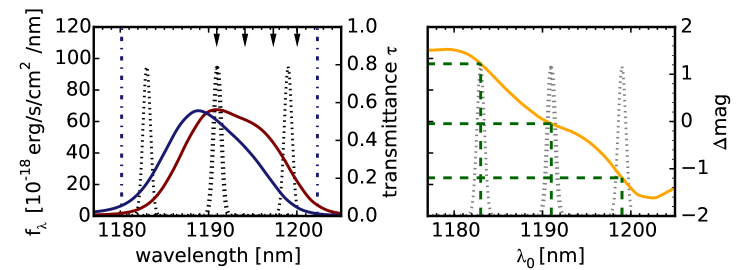
However, there is a problem when trying to estimate line fluxes from a single NB observation because the observed flux depends on the wavelength of the line. This problem can be understood from the left panel of Fig. 1 for the hypothetical example of a line without continuum. It is not possible to constrain both and , leading to order of magnitude uncertainties on the flux measurement. Further, the accuracy of the central wavelength estimation is limited to ’somewhere within the passband’, which might be for 1% filters, depending on the redshift, not much improvement over state of the art photometric redshifts.
Only if the NB filter’s passband was top-hat and if it was wide compared to the typical line width, the precise value of could be ignored for the flux estimation. Effective top-hat filters are however in the fast convergent beams of large survey telescopes such as VISTA, CFHT, and UKIRT physically impossible (cf. also Appendix A).
2.2 Observations with several NB Filters
One way to solve the problem described in sec. 2.1 is to use observations in more than one, slightly differing NBs. Then, two magnitude equations (eq. 3) are available for determining the two unknowns, and . can be eliminated from the equation, which can subsequently be numerically solved for as a function of the measured magnitude difference between the two filters, , as illustrated in Fig. 1.
With a well matched pair of NB filters, it is possible to determine the wavelength of a line within the range of wavelengths covered by the passband of the NB filter very accurately. Suitable filter pairs are those that result in – relations that are monotonous and steep, allowing for a good wavelength resolution, even when considering realistic uncertainties in .
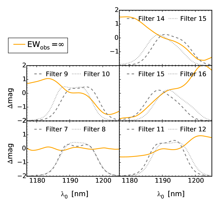
By means of such curves we characterized the suitability of the various combinations between the 16 UltraVISTA NB118 filters for our method to determine the line fluxes from two filters. As discussed in more detail in sec. 5.1, for 12 out of the 120 theoretically possible combinations of these 16 filters, observations become directly available as part of the standard UltraVISTA observations. One of these combinations is 14 & 15, which was used for illustration in Fig. 1.
While this specific pair is very well suited for the method, not all the possible NB118 combinations are so in the same way. In Fig. 2 four further of the 12 relevant NB118 combinations are shown, where 15 & 16 is as good, and 9 & 10 almost as good as 14 & 15. The two filters 7 & 8 are too similar to be useful for the presented method, whereas in the - curve of 11 & 12 still some information is contained. A quantitative characterization of the - curves for all 120 combinations is given in Appendix B.
2.3 Continuum estimation
In sec. 2.2, we have discussed the throughput variation method neglecting the continuum. But the continuum contributes for typical emission line galaxies significantly to the flux in NB filters. Hence, the magnitude differences measured for emission lines with the same and also depend on the equivalent width, .
A measurement of the contribution of the continuum to the NB fluxes is required; consequently, continuum-corrected NB magnitudes can be used to estimate and from the - curves for infinite . An accurate continuum estimate at the wavelength of the NB filter could be obtained from measurements in additional narrowband or mediumband filters bracketing the main NB filter. Typically, for reasons of time and cost efficiency, it is resorted to BB filters. If a BB which has a passband covering the emission line is included in the estimation, , , and need to be estimated simultaneously and the - curves cannot be used directly. We describe a statistical approach of fitting the parameters in the next section.
3 Estimation algorithm
3.1 Concept
- curves, as motivated in section 2.2, allow to get a quick insight into the suitability of a specific filter-combination for the throughput variations methods (TPV). In this section, we describe how to infer central wavelength, , line flux, , and equivalent width, , simultaneously using a statistical approach.
From the observation in the different filters, which can in principle include more than two NB filters, a set M of observed magnitudes, , and estimates on their uncertainty, is obtained. A model relates a set of parameters, , to a spectrum, , from which synthetically model magnitudes in the relevant filters, , can be calculated.
Then, the parameter set being most probable under these data needs to be found (). This is to minimize the Bayesian posterior probability . is related to the Likelihood, , and the prior on the parameters, , by:
| (4) |
is a normalization constant. As we are assuming the errors in the measurements of the different magnitudes to be independent and Gaussian, the total likelihood is given by the product of the normal distributions for the individual measurements. Consequently, the negative log-likelihood is 1/2 the well known :
| (5) |
The weight of individual filters can be artificially decreased by increasing the respective in the calculation of . In practice we chose a minimum for the broadband filters, , which we default to . The implications from this choice are analyzed in sec. 4.3.2.
3.2 Choice of input model
3.2.1 Continuum shape
Both the continuum shape and the ratios between the various emission lines will differ from galaxy to galaxy, even so they are selected by the combination of NB excess and photometric redshifts to be star-forming galaxies at a well defined redshift. If is parametrized by eq. 1, educated guesses need to be made for and . Ideally, these generic choices for and approximate the range of actual spectral energy distributions (SED) so well that the estimation of the free parameters is not impacted.
While the simplest form for is a continuum flat in or , a useful first order correction is to add an additional parameter in form of the power law slope (). This inclusion of the slope is especially relevant when the NB is off-centre from the BB passband, as it is the case for NB118 and J (cf. Fig. 20).
A power law continuum will not be sufficient if the wavelength range around the considered line includes a strong spectral break, like the break in the case of [O ii], but is a good assumption for in the NB118 filters, as discussed in sec. 4.2. We will address the problematic of the break on selection and measurement of [O ii] emitters in the NB118 data as part of a forthcoming publication.
3.2.2 Line shape and [N ii] contribution
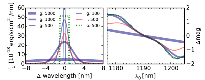
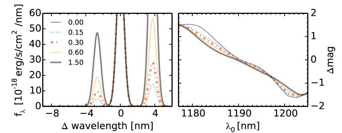
When observing in a NB filter, there is contamination from the collisional excited, forbidden [N ii] lines at and , which have to be included in . In the NB118 filters, where is observed at a redshift of , the lines are at a difference of and from , respectively. While the ratio between the fluxes in the two [N ii] lines, , is theoretically fixed to (Osterbrock 1989, p.61), the flux ratio does substantially differ from galaxy to galaxy. Values vary for pure star formation depending on the metallicity and the ionization parameter between 0.0 and almost 1.0 (e.g. Kewley & Dopita 2002), with even higher ratios possible for spectra with AGN contribution (e.g. Kauffmann et al. 2003a). Based on low redshift data, a typical value has been shown to be (e.g. Pascual et al. 2007 and references therein). In the absence of knowledge about the metallicities, correlations between and or mass can be used for a more sophisticated estimate. Using such relations in our estimation might bring some improvement, which we consider for further investigation. Throughout this work we assume a ratio of 0.3.
A wrong assumption on naturally impacts both the and estimation, where the impact on the latter can be examined by comparing curves for different . Curves for five different between and are shown for the example filter combination 14 & 15 in the lower panel of Fig. 3. We can conclude, while the impact is not negligible, the resulting systematic wavelength errors are even in the worst case not larger than , compared to the assumption of .
In addition to , also the shape of the line could differ.333We assume that the [N ii] lines have the same width as the line. Whereas line widths beyond are not expected for solely star-forming galaxies, line widths of several are possible when originating from a type I AGN. AGNs can be recognized by the use of the extensive multi-wavelength data available in fields like COSMOS.
We tested the impact of the line width on the estimation by determining curves for Gaussians with of 100, 500, 1000, , as shown in the upper part of Fig. 3. While a line with a width of several skews the result as expected, the difference all the way between and does not strongly impact the parameter estimation. Only, if the line had broader wings than a Gaussian, the deviations will be visible at lower . A boxcar line gives essentially an identical curve as a Gaussian with the same , but a Lorentzian will cause stronger deviations from the estimated wavelength especially at low filter transmittances. In the following, we assume throughout a default of . The impact of this specific choice is not expected to be large, as can be concluded from the results in this section.
3.3 Choice of broadband filters
In order to put an observational constraint on the continuum slope , at least two flanking BBs need to be used. This is in the case of the VISTA NB118 filters in addition to J naturally Y, but also H might be included, allowing for a stronger constraint on . For the analysis presented in the following we use all three filters.
As Y and H alone are theoretically enough to constrain a power law continuum, and any strong emission line in the NB118 filter also contributes to the flux in J, J can in principle be used as an estimator of the emission line flux. Whether it is actually feasible to obtain an accurate estimate from the J excess depends on two main criteria:
First, the contribution of the line to the filter-averaged signal needs to be high enough compared to the total noise in J. For the UltraVISTA DR2 data the S/N for an infinite EW line is in J a factor 4.1 lower than e.g. at the peak of NB118 filter 15 (For more details see Appendix D). Therefore, for the faintest lines detectable in the NB filter, the J-based estimate will not be very useful.
Secondly, it needs to be possible to determine the continuum contribution to with very high precision. For example, an line has a J excess of only , while the same object causes an excess of at the peak of NB118 filter 15. Hence, deviations between estimation power law and actual continuum SED are for fluxes measured through the broadband excess more critical.
3.4 Implementation of estimation code
| a𝑎aa𝑎a | b𝑏bb𝑏b ) | a𝑎aa𝑎a ) | ||
| start | 1170 | -17 | -1 | -3 |
| end | 1210 | -15 | 2.5 | 5 |
| steps | 15 | 10 | 10 | 8 |
Finding the right, global, maximum in a complicated probability landscape is not always easy. We implemented two versions of a python code to determine the parameter-set maximizing the posterior probability for a given set of measured magnitudes, M.
One version of our code makes use of the implementation of the Nelder-Mead algorithm (Nelder & Mead 1965) within python/scipy.minimize. Using the downhill simplex method, it allows to efficiently determine the maximum.555More precisely, the code searches for the minimum of the negative log-probability. In order to improve the success rate of finding the global maximum, we combined it with a pre-calculation on a coarse grained grid. The parameter-range of this pre-grid is given in Table 1. Then, we run the Nelder-Mead algorithm three times, starting from the grid points with the three highest probabilities. After comparing the found posterior probability from each run, we assumed in case of differing maxima the found maximum with the highest probablility as the global maximum and designated the corresponding parameters as . If all three sub-runs were not converging, or if for the best-fit parameter set was within of the prior boundaries, we assumed the parameter estimation as failed.
The Nelder-Mead implementation is relatively efficient, but it does not allow for a direct assessment of the credibility intervals. When having actual observations, where the experiment cannot be repeated as in simulations, the correct way to state uncertainties is to determine the posterior probabilities, e.g. based on a Markov chain Monte Carlo (MCMC) approach. Therefore, we implemented also a version based on the Metropolis-Hastings algorithm (Metropolis et al. 1953; Hastings 1970). The code makes use of adaptive proposal distributions based on repetitively recalculated covariance matrices, allowing for optimal efficiency (Roberts & Rosenthal 2001; Rosenthal 2014). We ran six separate chains with 100k proposal steps in each chain, where the initial proposal distribution was chosen wide enough to explore the complete parameter space.
Altogether, the set of four free fitting parameters, p, does include the central wavelength of the main line, , its integrated flux , the observed frame equivalent width, , for the main line, and the slope of the continuum. Within the prior, we constrained to a physically reasonable range in order to exclude combinations of unreasonably high and at low transmittances of the filters.
The range of acceptable was set for our specific test case of in the NB118 filters to and , respectively. Further, we constrained .
Assuming a flat prior for the line flux is from a rigorous Bayesian point of view not the right choice, as this does not reflect our complete state of prior knowledge. The line-luminosities are known to be approximately distributed by a Schechter luminosity function (LF) (Schechter 1976; z=0.8 LFs: e.g. Villar et al. 2008; Sobral et al. 2009; Ly et al. 2011). However, for clarity of the results we still use flat priors in this work.
4 Application to simulated observations
4.1 Mock observations
For testing the proposed TPV method systematically, we were using in this first part simulated observations for a range of spectra. The inputs into the simulation were chosen to closely resemble the available UltraVISTA DR2 data. This means that we used as inputs VIRCAM filter curves, the characteristics of the VIRCAM IR-arrays (gain, zeropoint (ZP)), and realistic sky brightnesses in the NB118 and the three VIRCAM BB filters.
The sky-brightnesses in the individual NB118 filters were taken from Milvang-Jensen et al. (2013) and significantly differ between the individual copies, ranging from to . For Y, J, and H we assumed 150, 650, , respectively, values typical for the UltraVISTA observations. We set the detector gains to and the ZPs on the AB system to 21.78, 24.12, 24.73, and 25.29 for NB118, Y, J, and H, respectively.666Based on Vega ZPs from http://casu.ast.cam.ac.uk/surveys-projects/vista/technical/photometric-properties and Vega to AB corrections calculated by us for the assumed filter curves.
Further, we were assuming point sources observed in 2″ diameter circular apertures. The corresponding enclosed flux fraction within the aperture is about for the UltraVISTA NB118 and J PSFs. For simplicity, the same enclosed fraction was also used for Y and H, even though the PSFs in these filters slightly differ for the actual observations.
Based on a chosen spectrum and these inputs, we synthetically calculated with eq. 3 the expected aperture magnitudes, , and from the corresponding signal-to-noise ratio (S/N) we derived by the expected magnitude errors.
The was estimated from the CCD equation (e.g. Howell 2000; Chromey 2010). Neglecting justifiably uncertainties from read-out noise, dark-current, linearity corrections, flat fielding, background subtraction, and converting electrons through the gain, , to digital-units, , the can be calculated as:
| (6) |
Here is the total number of per second created within the aperture due to the source, while is the number of produced per pixel and second by the sky-background. is the number of pixels constituting the aperture and is the exposure time.
We assumed an observation time of in each of two NB118 filters through which an object is simulated to be observed, which sums to the typical per-pixel integration time available in the UltraVISTA DR2. The expected per-pixel integration time in the finished survey will be , meaning that the DR2 NB118 data includes only % in time or 45% in depth of the final UltraVISTA survey goal. Similarly, we assumed for Y, J, H the 53.2, 34.9, 29.4 hrs available in the DR2 for the same field as the NB118 data, with the time in the finalized survey expected to be in each of the BB filters, all per pixel.
| Parameter | Values |
|---|---|
| Stellar population: | BC03 (Bruzual & Charlot 2003) based on |
| STELIB (Le Borgne et al. 2003) | |
| (BC03 based on BaSeL3.1 | |
| (Westera et al. 2002)) | |
| Nebular emission: | Recipe based on Schaerer & de Barros (2009); |
| Ono et al. (2010) | |
| IMF | Salpeter |
| Metallicities Za𝑎aa𝑎a | 0.008, 0.02, 0.05 (0.004, 0.008, 0.02, 0.05) |
| b𝑏bb𝑏bAge of the universe at was () | with 14 steps |
| ( in steps of 0.1) | |
| c𝑐cc𝑐cWe assume that the covering fraction of the gas, , is related to the escape of the ionizing radiation, , through | 0 (0.7,1) |
| d𝑑dd𝑑dExtinction assuming Calzetti et al. (2000) extinction law. The stellar extinction is assumed to be a factor 0.7 lower than the nebular extinction. | 0.2 ( in steps of 0.02) |
| SFH: | ( in steps of 0.2) |
| e𝑒ee𝑒eParameter of Dale & Helou (2002) models used for dust emission. | None (1.75) |
While we tested correctness and stability of our estimation code by using spectra as input models, which could be exactly matched by the estimation model, the mock observations used in the following were based on realistic galaxy SEDs. For the tests we used the high resolution BC03 models (Bruzual & Charlot 2003) based on the STELIB (Le Borgne et al. 2003) library assuming a Salpeter IMF (, Salpeter 1955).
4.2 Quality of continuum estimation from simulations

In the TPV estimation we use three BB filters, Y, J, H. This means that a relatively large wavelength range is included. The range from the blue end of Y to the red end of H corresponds at to a rest-frame wavelength range from to .
When estimating and from the throughput variations, the constraints on the continuum at the wavelength of the NB filter need to be precise. Further, as is also contributing to J, an excess in J impacts the estimation results with the algorithm described in sec. 3.1. Hence, the continuum needs also to be precisely estimated averaged over the complete J passband.
Therefore, it is important to carefully assess the expected deviations between the power law fit and the actual continua both in NB118 and J. Features in the spectral energy distributions (SEDs) could in principle results in such deviations. These are not necessarily of the same extent exactly at the wavelength of in the NB118 filter and averaged over J, especially as the NB118 passband is at the blue end of the J passband.
While no strong spectral features are expected over the covered wavelength range, only a formal test can give a clear answer. Therefore, we fit power law continua to synthetic magnitudes calculated for a grid of model SEDs without nebular emission included (Table 2). For consistency, we had scaled all input model SEDs to at the wavelength of , before calculating input magnitudes and uncertainties as in sec. 4.1.
In Fig. 4 the difference between the continuum magnitude at from the best-fit power law continuum, , and that measured directly from the input SED, , is shown for a range of SEDs. was determined by averaging the flux-densities over two wide intervals at and , corresponding to rest-frame wavelengths of and , respectively. These were chosen to exclude absorption. On the other axis, the differences between input and estimation are shown for . We conclude that the deviations averaged over the J passband are of similar extent as those for the continuum magnitudes directly at .
Both for stellar populations with solar and sub-solar (Z=0.4) metallicity these deviations are very small. Except for very young ages and for populations without ongoing star formation, the differences between fit and input magnitude are below . On the other hand, strong deviations exist for super-solar metallicities, exceeding for expected population ages. While this is cause for some concern, star-forming galaxies with stellar metallicity as high as are expected to be very rare (e.g. Gallazzi et al. 2014, at ), even at highest masses. Most of the NB selected galaxies will have stellar masses (e.g. Kochiashvili et al. 2015) and hence not be among the most metal rich systems according to the mass-metallicity relations (e.g. Tremonti et al. 2004; at : Savaglio et al. 2005; Lamareille et al. 2009). 888Typically stellar metallicities are, at least for local galaxies, below the gas-phase metallicity (Gallazzi et al. 2005).
We can conclude that the continuum estimate is expected to be excellent, making both the TPV and, at least to some extent, also the use of the J excess feasible.
4.3 Quality of full parameter estimation from simulations
We assessed the expected accuracy of estimations at different wavelengths for different and , different filter combinations, and different assumptions in the estimation algorithm. For this purpose we created in each considered case 500 realizations of observed magnitudes: we calculated for a given input spectrum the synthetic magnitudes and uncertainties, and randomly perturbed each of the magnitudes.999More precisely, we added the random noise to the flux densities.
Then, we ran our Nelder-Mead TPV code (cf. sec. 3.4) on each of the realizations. In this way, we found the expected distribution of best fit parameters for hypothetical repeated observations of the same object. Finally, the determined 4d distributions in the space were reduced to 1d distributions for each of these four parameters by marginalization over the three other parameters.
In all cases we used as input continuum a constantly star-forming solar metallicity SED with and an age of . This SED might be considered as a typical example for the emitters selected in the UltraVISTA data. The expected offset between power law continuum and this model continuum is marked in Fig. 4 as a cross. It is important to note, that this chosen continuum SED has an absorption of at .101010Measured from the SED with IRAF/splot Therefore, even perfectly estimated emission fluxes, , are too low by 16%, 8%, 5%, 3%, and 1% for emission with of 4, 7, 10, 20, and , respectively, as the TPV code does not correct for the absorption.111111The factors were calculated assuming an additional [N ii] contribution with . As the measured contribution of the [N ii] lines is for the actual NB118 filters redshift dependent, the expected underestimation factors also depend somewhat on the redshift. We added an line with chosen and to this continuum. The continuum was scaled so that the added line has a specific . We remark that adding to a somewhat arbitrary continuum is not completely self-consistent, but using the same continuum allows for a clear comparison of the results.
Line fluxes refer in the simulation parts of this paper to total fluxes, even though all measurements and estimations are simulated to be performed within the 2″ apertures.
4.3.1 Different line parameters
| A | B | C | D | A | B | C | D | ||
| Different input fluxes (Fig. 5) | |||||||||
| 3a𝑎aa𝑎a | ( | ( | ( | ( | |||||
| 5a𝑎aa𝑎a | ( | ( | |||||||
| 8a𝑎aa𝑎a | ( | ||||||||
| 15a𝑎aa𝑎a | |||||||||
| 30a𝑎aa𝑎a | |||||||||
| Different input EW (Fig. 6) | |||||||||
| 4b𝑏bb𝑏b | ( | ( | |||||||
| 7b𝑏bb𝑏b | ( | ||||||||
| 10b𝑏bb𝑏b | ( | ||||||||
| 20b𝑏bb𝑏b | ( | ||||||||
| 100b𝑏bb𝑏b | ( | ||||||||
| Different assumptions in the estimation (Fig. 7) | |||||||||
| c𝑐cc𝑐c | ( | ||||||||
| d𝑑dd𝑑d | ( | ||||||||
| eff.e𝑒ee𝑒eone NB118 filter; assuming effective combined NB118 filter 14 + 15 | ( | ||||||||
| Different filter pairs (Fig. 8) | |||||||||
| 14/15 f𝑓ff𝑓fFilter pair | ( | ||||||||
| 7/8f𝑓ff𝑓fFilter pair | ( | ||||||||
| 11/12f𝑓ff𝑓fFilter pair | ( | ||||||||
|
|
|
|
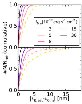
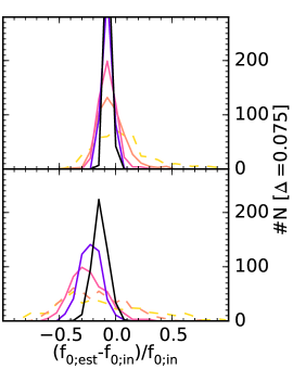
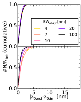
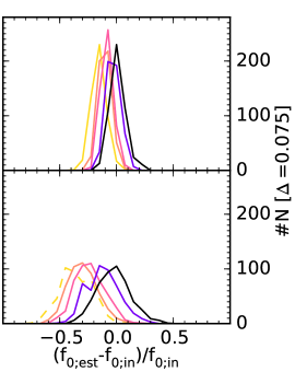
Ideally, a robust parameter estimation is possible for the complete range of existing in objects selected to be NB118 emitters. Therefore, we performed tests based on mock observations for a set of five input line fluxes, , over the complete relevant flux range from and for five input over the range from . In the two cases, we fixed the respective other quantity to and . Throughout this section we were assuming observations in filter combination 14 & 15, which is well suited for the TPV.
The resulting marginalized distributions for the best fit and are presented for each of the input combinations at two different input wavelengths in Fig. 5 and 6. Mean and standard deviation of these distributions are stated in Table 3.
The two wavelengths correspond to the mean wavelength of the two filter’s combined effective passband and the wavelength where the transmittance of this passband is 50% of its peak value. The mean wavelength was calculated as in eq. 6 of Milvang-Jensen et al. (2013). Table 3 includes results for two additional wavelengths. One is in the middle of the interval between mean wavelength and the 50% transmittance, and the other is at 20% transmittance. The four wavelengths are indicated as small arrows in Fig. 1.
We note that not for all combinations objects would also be selected as NB excess objects when applying selection criteria (cf. sec. 5.3.1), either because of not having enough S/N or not a high enough NB excess. These cases are indicated both in the plots and the table.
Several important things can be inferred from this analysis. The bias in the estimation is for all those among the tested combinations, which would be selected as NB excess objects. Further, the spread in the estimation, , is in all cases with selection below . For the spread is even over the complete relevant range, with little dependence on the .
While the seems to significantly change with , it is important to keep here the absorption in our assumed model SED in mind. At the mean wavelengths of the combined effective filter almost all apparent bias is only for this reason, whereas at lower transmittances there is some additional bias. This additional bias is resulting from the mismatch in the continuum.
4.3.2 Different estimation assumptions
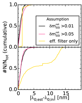
|
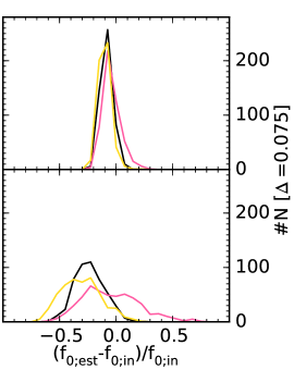
|
As discussed in sec. 3.3, the J excess is providing a flux estimate, as Y and H alone allow for a very good continuum estimate. In the case of a single NB118 filter, this would be supplemented by an additional lower limit on the flux. Therefore, one might wonder how much additional estimation power is really coming from the use of two NB filters.
In order to asses this, we performed the parameter estimation simulation for a galaxy with of and an line with of using the three BB filters either combined with the pair 14 & 15 or a single NB118 filter. For the latter we assumed the combined effective filter for 14 & 15. While this does not correspond to an actual filter, it is the applicable wavelength response when analyzing a joint stack of data coming from both 14 & 15.
Estimation histograms for both cases are shown in Fig. 7. Clearly, the use of the throughput variations between the two NB118 filters allows for an excellent estimation over the complete relevant wavelength range. By contrast, no robust estimation is possible when using only the single filter.
This is due to two main reasons. First, while in principle a wavelength resolution is possible when combining one NB filter with the flux measured based on a BB filter, a bimodality between a blue and a red solution is unavoidable. Secondly, at 50% transmittance another effect is obvious. As for the specific continuum SED, the continuum magnitude is estimated slightly too bright, the flux which is estimated from the J excess alone is underestimated. Therefore, even for a line several away from the peak, the lower limit from the NB filter indicates a stronger flux than estimated from the excess in J. Hence, the best possible reconciliation with the NB excess is for the estimation algorithm a solution being at the peak of NB filter. This is why the cumulative histograms in Fig. 7 jumps at around .
The difference between using the two NB filters separately and using the single combined effective filter is not as dramatic for the flux estimate, but still results in a huge improvement. At 50% transmittance, where the line still contributes significant signal to the NB data, the reduction of the bias due to the two NB filters corresponds for our standard to a factor of 1.3. At higher NB transmittances the effect is even larger. Halfway between the combined filter’s mean wavelength and 50% transmittance (cf. ’B’ in Table 3) it is a factor of 1.6. The difference is at transmittance negligible (cf. ’D’ in Table 3), as at the corresponding low transmittances in the NB filters the flux estimation is mainly relying on the J excess. Objects at this wavelength would not be part of our NB excess sample at the given .
We also investigated the consequences of increasing to , i.e. giving less weight to the BB filters. Clearly, the bias is significantly reduced. Even at transmittance, the bias is close to zero, keeping in mind the absorption. On the other hand, the scatter is significantly increased.
4.3.3 Different filter combinations
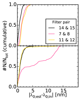
|
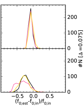
|
As a third test, we compared the estimation quality for three different filter combinations, including 14 & 15, which was used throughout sections 4.3.1 and 4.3.2, 7 & 8 and 11 & 12. All three combinations were discussed through curves in sec. 2.2. The pairs are well suited for a fair comparison, as the sky-brightnesses are with 36 & 32, 38 & 30, 33 & , respectively, similar in the three pairs.
The resulting distributions for the three different filter combinations, simulated for an line with , are shown in Fig. 8. It needs to be noted that both 7 & 8 and 11 & 12 are more top-hat than 14 & 15, which means that a one filter estimation is correct over a larger wavelength range.
We are showing in Fig. 8 the histograms for the mean wavelength and the 50% transmittance for the respective combined effective filters.
Combination 7 & 8 behaves as expected overall similar to a single effective filter, meaning that it is not very useful for an improved wavelength resolution. The wavelength resolution from 11 & 12 is also not as precise around the peak as for 14 & 15, as the curve is relatively flat there. At intermediate transmittances, where the slope is similar to that of 14 & 15, the wavelength resolution is on the other hand similar good.
5 Application to UltraVISTA data
5.1 UltraVISTA NB118 observing pattern

VISTA NB118 narrowband observations are already available from the NB118 GTO observations (Milvang-Jensen et al. 2013) and the intermediate UltraVISTA data releases (McCracken et al. 2012)131313McCracken et al. (2012) are describing the UltraVISTA DR1. The current release is DR2: www.eso.org/sci/observing/phase3/data_releases/uvista_dr2.pdf, and more data is continuing to become available within the ongoing UltraVISTA observations.
Interestingly, some parts of the covered field are becoming directly applicable to our method. VIRCAM covers with a single pointing a non contiguous area on the sky that consists of 16 separate patches, corresponding to the individual detectors. They total (Ivanov & Szeifert 2009, p.11). This single-pointing field coverage is referred to as a pawprint. In order to cover an area on the sky contiguously, a so called tile consisting of six pawprints is required.
The six contributing pawprints are three steps in one direction of the sky (y), which are performed for two steps in the perpendicular direction (x). For the NB118 part of UltraVISTA, only one of the two x-positions is observed, resulting in four stripes (cf. Fig. 9).
Each pointing in the y-direction is separated by 47.5% of a detector (or 5.5′).141414Each of the 16 detectors is a 2048x2048 Raytheon VIRGO HgCdTe array. 100% of a detector corresponds with the average pixel-scale of to 11.6′. Consequently, observations of at least two pawprints contribute to the covered field with the exception of the outermost parts. The filter numbers in the different patches of the pawprint can bee seen in Fig. 9. Most important for our method, in 20.5% percent of the stripes two pawprints contribute with two different filters. In addition for 6 tiny patches, which total 4.8% percent of the stripes, two pawprints contribute with one filter, while one pawprint contributes with a second filter. Due to the random jitter within a box, the regions are somewhat smeared out.
5.2 Data
The controlled environment of our simulations demonstrated that the TPV is expected to work. Here, we apply the method to the actual UltraVISTA DR2 data. A stack of NB118 data is available as part of this data release. In regions of overlap, this stack includes data from both contributing NB118 copies. For the purpose of the TPV, we need these data separately. Therefore, we produced 16 custom NB118 stacks, each of which including only the data from one filter/detector. Reduction, stacking, and flux calibration were basically done in the same way as for the publicly available joined NB118 DR2 stack (cf. Milvang-Jensen et al. 2013; McCracken et al. 201299footnotemark: 9) and the same observations were included.
Employing SExtractor’s (Bertin & Arnouts 1996) double-image mode, we obtained in each of the individual NB118 filters photometry in the same 2″ circular apertures as in the detection image, where the latter was the joined NB118 DR2 stack including data from all 16 filters. Matching dual image photometry was also obtained for the Y, J, and H DR2 stacks. We corrected all SExtractor aperture flux and magnitude errors for correlation by means of empty aperture measurements. This was necessary, as the stacks were produced on the non-native 0″.15 pixel scale and interpolation was required in the reduction as a consequence of the dithering strategy.151515Correlation corrections were previously determined based on UltraVISTA DR1 data. Stated observed magnitudes are aperture magnitudes in 2″ and are written in italic, where is referring to the magnitude in an individual NB118 filter and is referring to the magnitude in the joint stack.
We corrected the aperture magnitudes in Y, H, and NB118 to the J aperture based on the enclosed fractions for point-sources. The NB118 per-detector aperture magnitudes were corrected taking into account that different pawprints contribute to different parts of the NB118 per-detector stacks. I.e., we make sure that the remaining small seeing and ZP variations in data from different pawprints are corrected.
5.3 Sample selection
5.3.1 Selection criteria
We used following criteria to select NB excess objects in the regions of overlapping filters.
-
•
Position in field:
Observed in at least two different filters (7) -
•
Color-cut, which must be satisfied in at least one of the two contributing NB118 filters.
(8) The index i refers generically to the number of this filter and the second filter in the pair is referred to as j.
-
•
Significance of NB excess at the four level () at least in one filter, which satisfies also eq. 8
(9) This criterion corresponds to the often used criterion (Bunker et al. 1995). is the one sigma uncertainty on the flux difference. A justification of the choices in eq. 8 and 9 is given in Appendix F.
-
•
Significance of NB118 detection in the second filter at the () level.
(10) -
•
Mask
(11) where are the coordinates of the object, and are regions which are excluded due to bright stars, reflections, being close to detector boundaries, and a defect region in detector 16. We require additionally that the SExtractor flags in both contributing NB118 filters and Y and J are smaller than 4.
is the broadband flux density corrected to the position of the NB118 filter and was calculated from in the usual way by eq. 3. was approximated, depending on the S/N in Y, and the color, as:
| (12) | |||||
| else if then | (13) | ||||
| else | (14) |
Color correction and selection criteria are based on those of Milvang-Jensen et al. (2013), but adjusted for the use of observations in two NB filters. Additional alterations include the use of flux uncertainties instead of magnitude uncertainties and a change of slope in the color correction. We justify the selection in some more detail in Appendix F.
5.3.2 The NBES sample
Our main NB-excess sample (NBES) was selected based on the criteria in eq. 7 – 11, resulting in 239 objects. Matching to the photo-z catalog of Ilbert et al. (2013), we can identify as the cause of the NB excess in 86 cases +[N ii] or [S ii], 56 H or [O iii], 28 [O ii], and six [S iii], where the redshift cuts of , , , and were applied, respectively. The remaining 63 objects could either not be matched to the Ilbert et al. (2013) catalog or do not have a photo-z within the four intervals. Based on a full simulation of the NB118 observing pattern, as presented in Appendix C, we expect for the selection criteria about emitters, where the number depends on the chosen literature luminosity function, the equivalent width distribution, and the distribution. In the final UltraVISTA data we expect to select about twice as many emitters within the same sub-field.
In addition to the NBES, we picked 100 comparison samples, each of which having in each of the filters the same number of objects as the NBES with the same stack distribution. More precisely, we split the range between into 40 bins. The objects in the comparison samples (CS) were randomly drawn from a selection, where we did by contrast to the NBES not impose a color-significance or color-cut. In order to completely avoid NB excess objects in the comparison sample, we also created stricter versions, where we imposed (SCS).
5.4 Statistical analysis of throughput variations
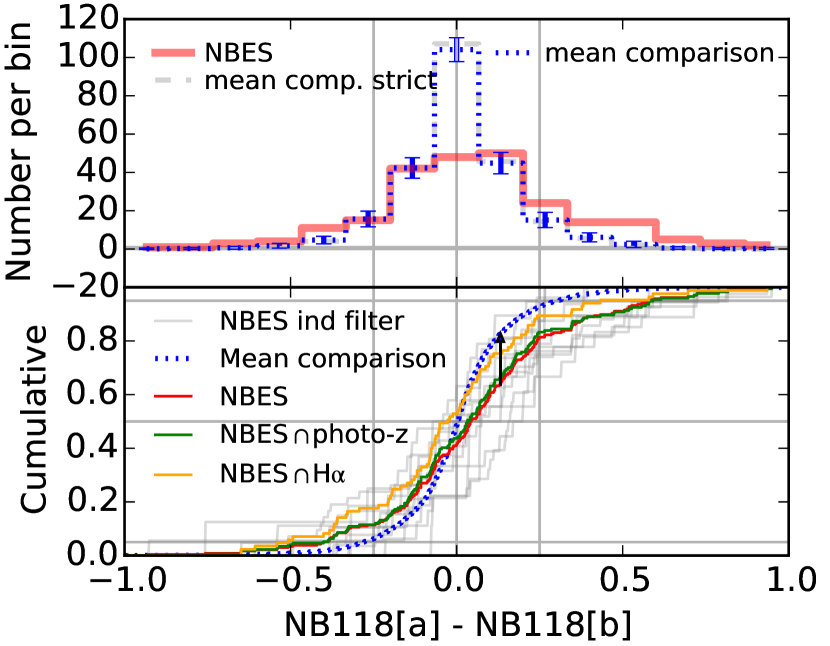
We tested whether we see at all NB excess objects showing throughput differences beyond the statistical fluctuations. In the upper panel of Fig. 10, the histogram of magnitude differences, , is shown as solid red curve for the NBES. All 12 filter combinations are included in the same histogram, where the identifiers and generically refer to the filter numbers in the pairs, with . Also included in the figure is the mean histogram of the 100 CS and the corresponding standard deviation. The SCS sample is indicated as a dashed light gray line, which is hardly visible as it is basically identical with the CS histogram.
Including predominantly objects without emission in the NB118 filters, the spread in the CS should be caused by noise only. By contrast, the spread in the histogram for the NBES is expected to be caused both by noise and actual throughput variations, and indeed, it clearly differs from the comparison sample. The difference can also be evaluated in the lower panel of Fig. 10, where the cumulative histograms are shown. Applying the two-sample KS test to the two histograms, we can formally rule out the null-hypothesis that both samples are originating from the same distribution.161616At the 99.999997% level; more precisely, the comparison sample used in the KS test was the combination of the 100 realizations, having effectively 100*239 objects. The maximum difference between the two cumulative curves is marked as an arrow in the figure.
One relevant concern is that objects with unusually large random or systematic errors in one of the two filters could show the required NB excess exactly for that reason, which might lead to a misidentification of such objects as NB excess objects and hence an inclusion in the NBES, biasing this sample to objects with large throughput variations. However, as discussed above and further shown in Fig. 11, photometric redshifts of 74% of the NBES objects can be well identified with actual lines, indicating a relatively clean sample. Reassuringly, the average cumulative magnitude difference curve does not change much using only this sub-sample (green curve in Fig. 10). For the subsample of emitters the difference to the general population is slightly smaller, being explainable as the most extreme NB excess objects are predominately [O iii] emitters.
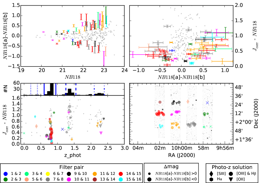
As a next step, we selected those objects from the main NB-excess sample (NBES), which show a flux difference between the two filters differing from zero at least at the level, have a , and are fainter than . The latter two criteria are meant to avoid objects, where the difference might be caused by small remaining zeropoint errors or by small PSF differences, being especially relevant for merging objects.
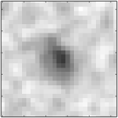
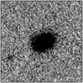
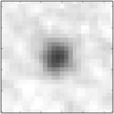
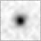
The resulting 55 objects, 8 of which are so close to a neighboring object that SExtractor marked them as de-blended171717SExtractor FLAGS = 2 or 3, are shown in four different plots in Fig. 11. While all objects of the NBES are included in the plots as gray dots, objects in the throughput difference sample are color-coded by the relevant filter pairs. Adding to the confidence that those objects with strong TPV are indeed NB excess objects caused by emission lines, a comparison of this subsample to the photometric redshifts of Ilbert et al. (2013) allowed in an even larger fraction than in the full NBES for an identification with one of the four main redshift solutions (85% vs 74%).181818For one of two [SIII] candidates, visual inspection of the SED allowed for an unambiguous identification with an extreme EW object at , showing a -filter excess corresponding to a rest-frame [OIII] + H equivalent exceeding The 8 remaining objects are classified in the Ilbert et al. (2013) catalog as either masked (2), star (1), XMM detected (1), a photo-z not in the intervals (1), or we could not find a match within a radius of 0.5″ (3).
While the number of objects is too small to make strong statistical conclusions for the individual filters, we find that strong throughput variations are indeed mainly found in those pairs for which they were expected (14 & 15, and also 15 & 16 and 9 & 10). However, there is one major exception. Filter pair 7 & 8 shows surprisingly (cf. Fig. 2) a relatively large number of objects with strong differences. With some of them being brighter in filter 7 and others in filter 8, an erroneous ZP can be ruled out as reason for the behavior. A visual inspection of the objects also does not indicate obvious problems. Therefore, we need to conclude that one of the two filters seems to substantially differ from our expectations (cf. also Appendix A).
5.5 NB118 H measurements for individual objects
| ID a𝑎aa𝑎aNBES | zCOSMOS b𝑏bb𝑏bzCOSMOS bright 20k (Lilly et al. 2009) ID | pairc𝑐cc𝑐ccontributing NB118 filters | d𝑑dd𝑑dH central wavelength [] (TPV) | d𝑑dd𝑑dH central wavelength [] (spec) | d,f𝑑𝑓d,fd,f𝑑𝑓d,ffootnotemark: (phot-z) | e𝑒ee𝑒e[] (TPV) | e𝑒ee𝑒e[] () | e𝑒ee𝑒e[] (H) | e𝑒ee𝑒e[] (total) | e𝑒ee𝑒e[] (SED) |
|---|---|---|---|---|---|---|---|---|---|---|
| 7 | 810332 | 15/16 | 1201.3 | 1201 | ||||||
| 14 | 15/16 | 1180 | ||||||||
| 33 | 810529 | 15/16 | 1199.1 | 1194 | ||||||
| 94 | 14/15 | 1199 | ||||||||
| 96 | 822610 | 14/15 | 1197.6 | 1186 | ||||||
| 97 | 14/15 | 1204 | ||||||||
| 99 | 822560 | 14/15 | 1189.9 | 1191 | ||||||
| 104 | 14/15 | 1201 | ||||||||
| 105g,h𝑔ℎg,hg,h𝑔ℎg,hfootnotemark: | 822732 | 14/15 | 1199.4 | AGN | ||||||
| 111 | 14/15 | 1197 | ||||||||
| 113 | 823319 | 14/15 | 1197.7 | 1186 | ||||||
| 114 | 822686 | 14/15 | 1193.2 | 1190 | ||||||
| 117g𝑔gg𝑔gChandra point source (Civano et al. 2012) | 822508 | 14/15 | 1194.7 | AGN | ||||||
| 121 | 822822 | 14/15 | 1197.3 | 1174 | ||||||
| 122 | 14/15 | 1197 | ||||||||
| 124 | 14/15 | 1188 | ||||||||
| 125 | 822496 | 14/15 | 1198.5 | 1190 | ||||||
| 126 | 14/15 | 1199 | ||||||||
| 128 | 14/15 | 1162 | ||||||||
| 131 | 14/15 | 1201 | ||||||||
| 135i𝑖ii𝑖i[Ne v] detected in zCOSMOS spectrum | 823097 | 14/15 | 1184.5 | |||||||
| 138 | 822504 | 14/15 | 1195.0 | 1186 | ||||||
| 147 | 14/15 | 1153 | ||||||||
| 150 | 14/15 | 1188 | ||||||||
| 153 | 14/15 | 1182 | ||||||||
| 161 | 14/15 | 1211 | ||||||||
| 164 | 14/15 | 1184 | ||||||||
| 167 | 823087 | 14/15 | 1191.7 | |||||||
| 170 | 14/15 | 1186 | ||||||||
| 172 | 09/10 | 1180 | ||||||||
| 186 | 839235 | 09/10 | 1197.6 | 1104 | ||||||
| 204 | 838539 | 09/10 | 1182.3 | 1141 | ||||||
| 205 | 838552 | 09/10 | 1181.6 | 1180 | ||||||
| 226 | 09/10 | 1201 | ||||||||
| 235 | 09/10 | 1185 |
| ACS (F814W) | Y (DR2) | NB118 14 | NB118 15 | J (DR2) |
| NBES 121 / zCOSMOS 822822 | ||||
 |
 |
 |
 |
 |
| NBES 135 / zCOSMOS 823097 | ||||
 |
 |
 |
 |
 |
5.5.1 Estimation with TPV
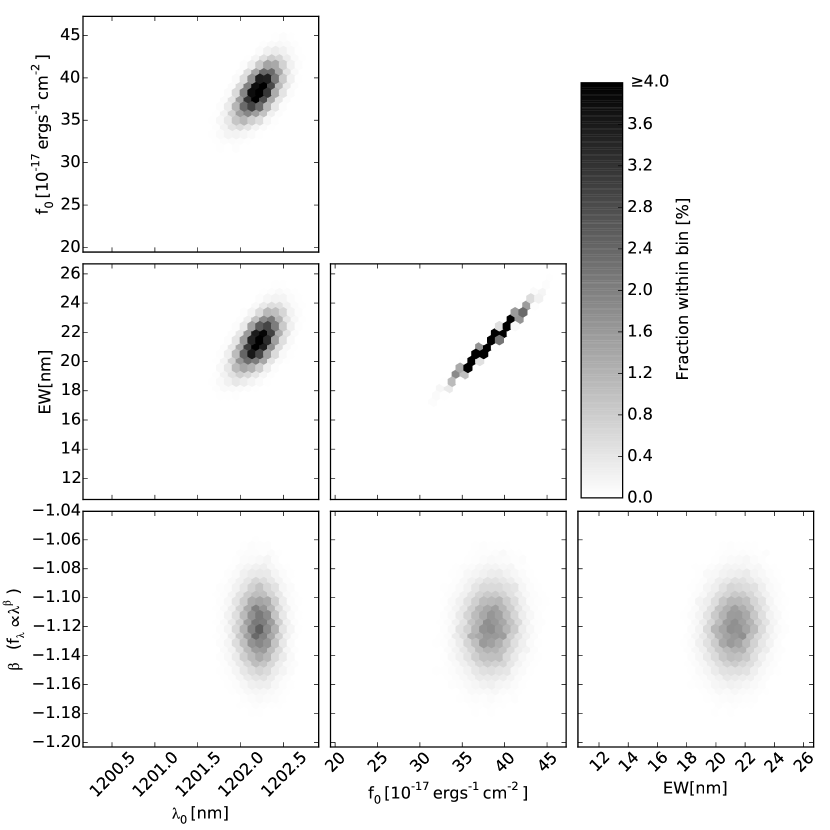
We applied our parameter estimation method to all those NB excess objects in our sample, which are located in one of the three filter pairs suited for our method (9 & 10, 14 & 15, 15 & 16) and which we classify as emitters based on their photo-z’s or their zCOSMOS redshifts (cf. sec. 5.6.3) being consistent with in the NB118 filter. We also verified the selection through the use of a versus plot, similar to Sobral et al. (2009, 2013). For all selected objects we estimated all flux (), central wavelength (), , and continuum slope (), and the corresponding uncertainties based on the MCMC implementation of our algorithm (cf. sec. 3.4). Estimated and for all objects are listed in Table 4. An example for the resulting credibility intervals is shown in Fig. 13 for the object with NBES ID 7, an object with high flux and being located at the boundaries of the passband. The statistical uncertainties are very small, but as discussed above, systematic errors are at least of the same order.
5.5.2 Estimation with generic NB118 method
For comparison, we also estimated fluxes with a conventional NB estimation method using the stack NB118 magnitudes. Here we used as estimator:
| (15) |
The effective filter width, , was determined for the combined effective filters using the approach described by Pascual et al. (2007)202020The relevant equations from Pascual et al. (2007) are especially 7 and 12.. In the we took account for the [N ii] contribution following the approach of Pascual et al. (2007). The were determined from the AB magnitudes in the common way. The used estimator is the simplest possible form, which assumes that the impact of the emission line to the broadband magnitude can be neglected.
5.6 Independent flux estimates
In order to asses the quality of our NB118 parameter estimation, we needed to compare to estimates of and from independent methods. While a direct comparison to J spectroscopy would be ideal, we had to rely in the absence of such data on information obtained from available optical spectroscopy and multi-wavelength photometry. This is, we obtained flux estimates in three ways:
-
1.
fluxes obtained from SED fitting
-
2.
Conversion of the total SFR obtained from UV+IR into fluxes
-
3.
Conversions between H and/or [O ii] fluxes from zCOSMOS spectra into fluxes
5.6.1 Estimation from SED fitting
We performed SED fitting using our own python code coniecto, which normalizes through a common minimization a set of models with respect to mass, and allows consequently to find the model allowing for the smallest . Our parameter grid was chosen fine enough to avoid biases due to degeneracies between different parameters. The full range of parameters is stated in Table 2.
As input we used the Muzzin et al. (2013) photometric catalog and included in total 29 filters in the fitting, from GALEX FUV to IRAC 4. The photometry in Muzzin et al. (2013) is based on 2″.1 diameter apertures applied to PSF homogenized images. We compared for each of the objects our 2″ aperture photometry for Y, J, H to that in the Muzzin et al. (2013) catalog.212121The Y, J, H data in the Muzzin et al. (2013) catalog is based on UltraVISTA DR1 data. On average, the difference in the magnitudes is with very small. We corrected all quantities obtained based on the Muzzin et al. (2013) photometry to match our apertures, which also crudely takes care of small differences in the centroid from our detection and that in Muzzin et al. (2013).
In addition to stellar continua based on BC03 models (Bruzual & Charlot 2003) using a Salpeter IMF, we also add dust and nebular emission to the models, including lines and continuum. For the dust emission we use the Dale & Helou (2002) models under the assumption of energy conservation, meaning that all radiation absorbed by dust must be reemitted. We remark that emission from dust, including PAH features, is in the IRAC bands at only of minor importance.
Throughout this and the following sections we consistently used a Calzetti et al. (2000) extinction law. The extinction of the stellar continuum, , was chosen to be 0.7 times the nebular extinction, . Calzetti et al. (2000) find based on a sample of local starburst galaxies (Calzetti 1997) a factor 0.44 between the two extinctions. On the other hand, under this assumption Erb et al. (2006) find a systematic discrepancy between and UV based SFRs at , with equal extinction for both components giving more consistent results, in agreement with some more recent studies (e.g. Shivaei et al. 2015). Other studies argue for differential nebular and stellar extinction also at high redshifts (e.g. Förster Schreiber et al. 2009; Wuyts et al. 2011). These discrepant conclusions can be partially explained by a SFR dependence of the ratio between nebular and stellar extinction, in a sense that the ratio is higher for higher SFRs (Price et al. 2014; Reddy et al. 2015). Our chosen value of 0.7 should be understood as a compromise. For , we use either the same as for all other lines or somewhat arbitrarily a ten times higher extinction. Finally, we apply IGM absorption to the SED models using the parameterization of Inoue et al. (2014).
We interpret the calculated grid in a Bayesian way (e.g. Kauffmann et al. 2003b; Benítez 2000; da Cunha et al. 2008; Noll et al. 2009). Assuming Gaussian errors, the likelihood is given by . As a prior is naturally imposed through the sampling of the grid, we can directly interpret the likelihoods as posterior probabilities. We determined the posterior probability distributions (PDFs) both for the input parameters and a range of derived parameters through marginalization over the other input parameters. Marginalization is realized by summing the posterior probabilities. While we determined the probabilities for the input parameters at the sampling points of these parameters, we binned for the derived parameters. Finally we determine the 68% confidence intervals, by excluding the first and last 16% in the PDFs. If the point of minimum is outside the 68% interval, we extend the uncertainty interval to include the minimum value. Uncertainties derived in this way are listed for the SED based estimates in Table 4 and for other SED parameters in Table 7.
As we are adding 5% of the flux to the formal flux-uncertainties, in order to reduce artificial impacts of possible ZP uncertainties and template mismatches, the stated uncertainties should not be over-interpreted.
5.6.2 Estimation from total SFR
For those objects with significant Spitzer/MIPS detection in the Muzzin et al. (2013) catalog, we obtained total SFRs from the sum of UV and IR based SFRs. While Muzzin et al. (2013) provide these values as part of their catalog, we can assume a more precise redshift and it is hence worth to recalculate the values.
We determined total IR luminosities, , by scaling the Dale & Helou (2002) templates so that synthetic MIPS magnitudes match the measured ones, and consequently integrating the scaled templates over the range from . Following Wuyts et al. (2008) we used as result the mean of the Dale & Helou (2002) models for between , where is the power law index, characterizing the fractional dust mass, , heated by a certain interstellar radiation intensity, U, meaning . Upper and lower limit of the stated uncertainties are given by the values obtained for and . It is noteworthy, that in the case of contribution from an AGN, the determined values will not be correct.
The total infrared luminosity can be converted into a SFR by (Kennicutt 1998):
| (16) |
For the unobscured UV SFR we determined first the the continuum luminosity density at a rest-frame wavelength of from our best fit SED model and converted this luminosity into a SFR by using (Kennicutt 1998):
| (17) |
Finally, we converted the determined total , being the sum of and , to fluxes, using the relation from Kennicutt (1998),
| (18) |
the generic relation between flux and luminosity for our assumed cosmology, and the nebular extinction obtained from the SED fit.
5.6.3 Estimation from zCOSMOS data
In addition, we were using redshifts and line fluxes from the zCOSMOS survey (Lilly et al. 2007, 2009). Matching the coordinates of our NBES objects to the zCOSMOS-bright 20k data-set222222The publicly available zCOSMOS-bright DR2 10k is a subset of this catalog. revealed an overlap of 35 objects with redshift information. It is reassuring that for all matched objects the redshifts confirmed the presence of an emission line within the filter, which is for 31 objects + [N ii]. The number of those emitters being in the three most useful filter pairs 9 & 10, 14 & 15, and 15 & 16 are 3, 11, and 2, respectively.
The zCOSMOS VLT/VIMOS spectra are covering the wavelength range from 550 to 970. This means that they include for an object with in the NB118 filter both [O ii], being unresolved in the VIMOS data, and H at observed-frame wavelengths of and , respectively, assuming .
We matched the zCOSMOS spectral fluxes to our imaging apertures by multiplying the continuum flux density at the lines’ wavelength obtained from the SED fitting with the respective zCOSMOS . In this way, we avoid slit loss and flux calibration issues, with some remaining discrepancy expected from the spatial distribution of H ii regions, if objects are more extended than the PSF.
The [O ii] fluxes can be converted into SFRs, using the calibration by Kewley et al. (2004):
| (19) |
This equation is for intrinsic, meaning reddening corrected luminosities. Therefore, we de-reddened the measured [O ii] fluxes as an intermediate step, again assuming the from the best fit SED. The obtained SFR was then converted into an flux using again eq. 18.
The ratio between [O ii] and is depending to some degree on metallicity and the ionization parameter (e.g. Moustakas et al. 2006). By contrast, H allows for a more direct conversion, with the additional advantage of a lower difference in reddening between the wavelengths of H and than between [O ii] and . Unfortunately, the H S/N is relatively low in the zCOSMOS spectra. For those objects with H detection at least at the 2 level, we obtained an estimate by converting between the reddening corrected values. The intrinsic ratio between and H is 2.86 for typical conditions in H ii regions, assumed to be and (Osterbrock 1989, p. 84).
5.7 Comparison of TPV with other estimates
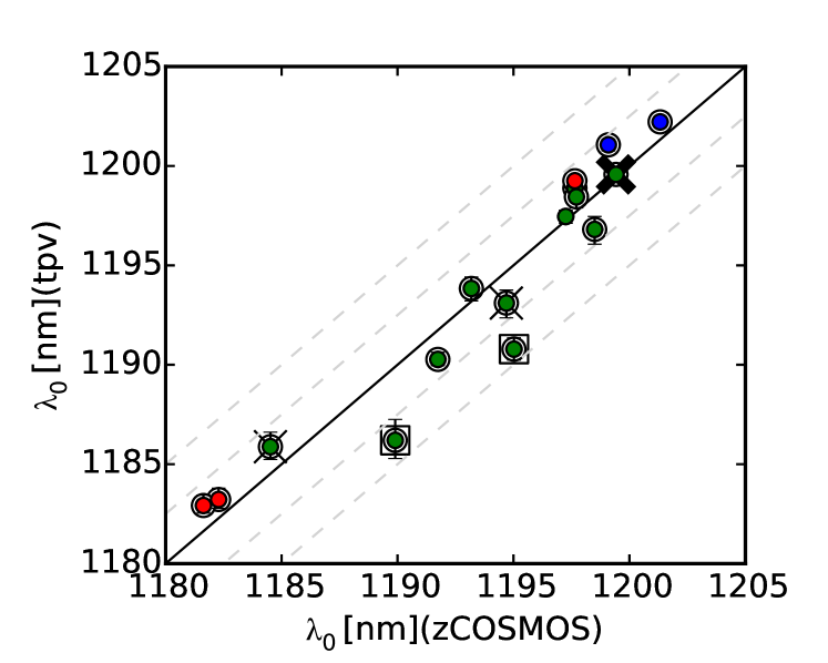
Using the zCOSMOS redshifts and the line flux estimates of sec. 5.6, we can now directly compare the TPV estimates with those from completely independent measurements and thereby measure the success of the TPV method. First, we consider the redshifts. Because of the high accuracy of the spectroscopic redshifts, the accuracy of the TPV estimates can be directly assessed with a straight forward comparison. In Fig. 14, the TPV estimates of the wavelength is plotted against the obtained from the spectroscopic zCOSMOS survey. It can be seen that the TPV wavelength estimates closely follow spectroscopic estimates, with a mean difference of and a scatter of . All except two objects are within . Excluding these two outliers, the scatter decreases to . We remark that the observed scatter is larger than the statistical error estimate from our estimation code. This indicates that the errors are dominated by systematic effects. Expected systematic uncertainties result from mismatches between true and estimation continua, discrepancies between true and assumed [N ii] ratios, and uncertainties in the available filter curves (cf. Appendix A).
Next, we consider the line flux measurements. In this case, individual independent estimates are not necessarily more accurate than the TPV estimates. For that reason, we combined UV+IR, SED, [O ii] and H based estimates by taking the mean of the individual values. In Fig. 15, the ratio of the NB118 line flux estimates to the combined estimates are plotted versus wavelength. The top panel shows the TPV estimates, while the bottom panel shows the generic discussed in Sec. 5.5.2. The same data is shown in a different way in Fig. 16. In this figure the ratios between the three different estimates can be directly assessed for individual objects.
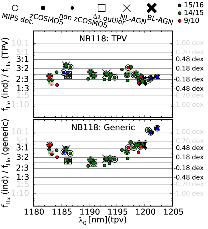
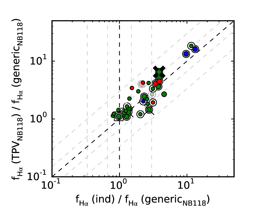
For several objects the UV+IR and the SED based estimates differ by more than a factor ten. The combined line flux for these objects is therefore uncertain, and these objects are shown faded in the figure. Specifically marked in the figure is one of the objects, which is according to the zCOSMOS flag 13.5 (cf. Lilly et al. 2009) a broad line AGN, and one object which shows [Ne v] in its spectrum and is hence identified as hosting a type II AGN (e.g. Mignoli et al. 2013). About 80% of the field with data from the filter pairs 9 & 10, 14 & 15, and 15 & 16 are covered by Chandra data from Elvis et al. (2009), out of which have deep coverage. Matching to the Chandra point source catalog (Civano et al. 2012) revealed one further X-ray detected object. We classify it for the plot as NL AGN. Our independent flux estimates for these objects with certain AGN contribution are only of limited usefulness.
The figure demonstrates that the agreement between the TPV and combined independent line flux estimates is good. The mean of the differences is with a standard deviation of . In particular, there is no trend with wavelength over the complete wavelength range of the bandpass. By contrast, the generic single NB filter estimate leads to substantially biased line flux estimates, that can underestimate the flux by as much as a factor of 10 towards the edge of the filter band. Such a bias would for example have significant impact on the investigation of the structure at wavelengths around (see sec. 5.8).
Overall, we conclude that our TPV flux estimates are robust and unbiased, and the error on the flux is by as much as a factor of 20 smaller than using generic single NB estimates to derive line fluxes.
5.8 Spatial and redshift distribution in example filter pair
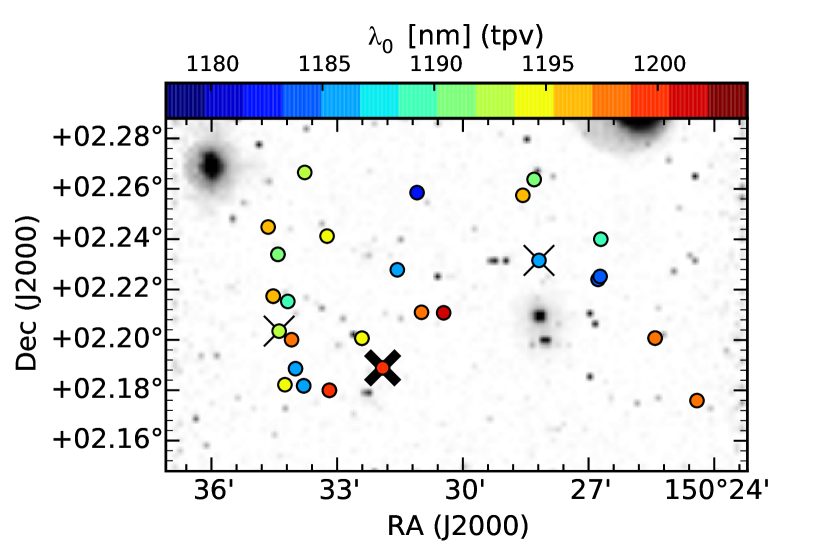
The use of the TPV method allows us to directly identify three dimensional structures, like filaments or sheets, the detection of which would otherwise require spectroscopic observations with sufficient resolution.
This is demonstrated in Fig. 17, which shows the spatial distribution of emitters observed with the filter pair 14 & 15, combined with the wavelength information obtained from the TPV. The size of one NB118 detector corresponds to a comoving distance of 9.7 Mpc at the redshift of in the NB118 filter, while the depth of the volume covered by the wavelength range from to is much larger, namely 103 Mpc comoving.232323Alternatively, expressing central wavelength differences as redshift velocities, corresponds to . Observations with a single NB118 filter can not resolve the depth of the field.
By contrast, the redshift resolution obtained with the TPV is sufficient to identify several objects that are at similar redshifts as the BL-AGN, revealing substantial clustering associated with the AGN. In addition, there are also several emitters within the field but at the other redshift end of the volume, i.e. they are spatially well separated from the AGN cluster. Finally, there is a string of objects towards the east. This feature includes objects at various redshifts, and is likely a sheet-like structure. While a deeper discussion of these structures is beyond the scope of this paper, this example demonstrates the amount of additional information which can be gained from the TPV.
5.9 Optimizing the observing pattern
As discussed in sec. 2.2, the best suited pairs have curves with average slopes in of and are monotonous over the relevant wavelength range. Unfortunately, the standard UltraVISTA observing pattern leads to only three cases where the same position on the sky is observed with such ideal filter combinations, namely the filter combinations 9 & 10, 14 & 15, and 15 & 16. One reason for this is that the filter arrangement within the VISTA camera was chosen to maximize the obtainable depth and hence the filters are as similar as possible within each column (Nilsson 2007; Milvang-Jensen et al. 2013). Therefore, the overlapping filters are in most cases more similar than the overall spread between the 16 NB118 filters suggests (cf. Fig. 19).
In order to make use of the full potential of the proposed TPV method, the observing pattern should be modified to increase the number of cases where repeated observations of the same field use dissimilar filters. One easy to implement strategy is to turn the telescope by 180° for half of the observation time. With this strategy, every observed position is covered by at least two filters, whereas in the standard observing pattern, about 75% of all positions are covered with only one filter. Furthermore, in the other patches, where already in the standard observing pattern two filters contribute, there would be data from four filters. This increases the number of combinations, which are different enough to allow for a good parameter estimation. Out of the 44 patches more than half (24) have an average slope of the curve larger than .242424The average slope was calculated as further described in Appendix B. For those patches, where four filters contribute, we calculated an average slope from the three largest slopes for all six possible combinations.
While the turning pattern would be an enormous step forward for the method, it comes at a prize. The specific positioning of similar filters is the logical step in order to maximize the reachable depth, being most crucial for one of the main science goals of the VISTA NB118 observations, the search for Ly emitters. We evaluated the impact of this loss in depth with the simulation described in Appendix C.1. This simulation takes account for the difference in filter profiles and background in the individual filters. In short, we randomly assigned positions on the sky and central-wavelengths to objects, simulated the observations, and determined the fraction of input objects which would be detected as a function of wavelength. Different from the selection criteria in sec. 5.3.1, we required here a color-significance in the complete stack instead of the two-filter criteria, and considered the complete field. To test effects of the finite number of simulated objects, we also tested the variance between 10 subsets of objects, and found negligible impact on the results.
In Fig. 18, the fraction of detected objects as function of the flux is shown both for the standard observing pattern and the turning modified one. There is clearly a non-negligible fraction of objects that will be missed at the very faint end when using the turning pattern. Therefore, deciding against or in favor of the turning pattern is a difficult trade-off.
6 Summary and Conclusions
In this paper, we have carefully demonstrated the usefulness of the TPV method to derive redshifts and line fluxes from wavelength dependent throughput differences between NB filters with slightly differing, yet overlapping passbands, and corresponding broadband filters. While it is possible to specifically design NB filters for this method, suitable filters and data taken with such filters already exist, e.g. the UltraVISTA survey taken with ESO’s VISTA/VIRCAM. For our analysis, we focused on the line in the narrowband NB118 filters of that survey. About 1/4 of the UltraVISTA field is covered by at least two different NB118 filters. We used simulations to assess the expected accuracy of our method given the current exposure time of the survey. We found that for the most suitable filter pair, the simulations predict that it is possible to measure wavelengths with random and systematic errors as low as for a line with independent of . The wavelength estimation results were also shown not to be strongly affected by assumptions on the line width and the required [N ii]/H ratio.
The accuracy in redshift compares favorable to photometric redshifts. A wavelength error of corresponds to a . By comparison, highest quality photometric redshifts in the COSMOS field can at best reach a resolution of about (e.g. Ilbert et al. 2013).
In addition to the simulations, we also applied the method to the actual UltraVISTA DR2 data. A comparison of wavelengths estimated with our method and those obtained from the spectroscopic zCOSMOS-bright 20k catalog (Lilly et al. 2009) shows an excellent agreement with a measured scatter of . This value is similar to the found by Hayashi et al. (2014) in their observations of a galaxy-cluster with two optical NB filters in Suprime-Cam on the Subaru Telescope. Independent predictions for the line flux, both based on spectroscopic [O ii] and H fluxes and photometric data, also confirm that the proposed method works very well and is a significant improvement compared to the results from a generic line flux estimation. This improvement is shown again in Fig. 16.
We therefore conclude that the TPV method is a powerful tool to derive redshift and flux estimates from NB surveys that employ multiple versions of similar filters. One of the advantages of the method is that it exploits information that is routinely collected with some instruments. The improvement over the standard analysis is as much as an order of magnitude reduction in the errors.
Acknowledgements.
We thank the anonymous referee for very constructive comments. The Dark Cosmology Centre is funded by the Danish National Research Foundation. JZ acknowledges support from the ERC Consolidator Grant funding scheme (project ConTExt, grant number 648179). BMJ and JPUF acknowledge support from the ERC-StG grant EGGS-278202. Part of this research was funded by an ESO DGDF grant to WF and PM. Based on data products from observations made with ESO Telescopes at the La Silla Paranal Observatory under ESO programme ID 179.A-2005 and on data products produced by TERAPIX and the Cambridge Astronomy Survey Unit on behalf of the UltraVISTA consortium. The zCOSMOS observations are based on observations made with ESO Telescopes at the La Silla or Paranal Observatories under programme ID 175.A-0839. This research made use of several community-developed Python packages: Astropy (Astropy Collaboration et al. 2013), Matplotlib (Hunter 2007), SciPy and NumPy (Oliphant 2007).References
- Astropy Collaboration et al. (2013) Astropy Collaboration, Robitaille, T. P., Tollerud, E. J., et al. 2013, A&A, 558, A33
- Atad-Ettedgui & Worswick (2003) Atad-Ettedgui, E. & Worswick, S. P. 2003, Specialized Optical Developments in Astronomy. Edited by Atad-Ettedgui, 4842, 95
- Benítez (2000) Benítez, N. 2000, ApJ, 536, 571
- Bertin & Arnouts (1996) Bertin, E. & Arnouts, S. 1996, A&AS, 117, 393
- Best et al. (2010) Best, P., Smail, I., Sobral, D., et al. 2010, eprint arXiv:1003.5183
- Bland-Hawthorn et al. (2001) Bland-Hawthorn, J., van Breugel, W., Gillingham, P. R., Baldry, I. K., & Jones, D. H. 2001, ApJ, 563, 611
- Bruzual & Charlot (2003) Bruzual, G. & Charlot, S. 2003, MNRAS, 344, 1000
- Bunker et al. (1995) Bunker, A. J., Warren, S. J., Hewett, P. C., & Clements, D. L. 1995, MNRAS, 273, 513
- Buser (1986) Buser, R. 1986, in IN: Highlights of astronomy. Volume 7 - Proceedings of the Nineteenth IAU General Assembly, Basel, Universität, Switzerland; Space Telescope Science Institute, Baltimore, MD, 799–804
- Calzetti (1997) Calzetti, D. 1997, AJ, 113, 162
- Calzetti et al. (2000) Calzetti, D., Armus, L., Bohlin, R. C., et al. 2000, ApJ, 533, 682
- Chromey (2010) Chromey, F. R. 2010, To Measure the Sky (Cambridge, UK: Cambridge University Press)
- Civano et al. (2012) Civano, F., Elvis, M., Brusa, M., et al. 2012, ApJS, 201, 30
- da Cunha et al. (2008) da Cunha, E., Charlot, S., & Elbaz, D. 2008, MNRAS, 388, 1595
- Dale et al. (2010) Dale, D. A., Barlow, R. J., Cohen, S. A., et al. 2010, ApJ, 712, L189
- Dale & Helou (2002) Dale, D. A. & Helou, G. 2002, ApJ, 576, 159
- Dalton et al. (2006) Dalton, G. B., Caldwell, M., Ward, A. K., et al. 2006, in Society of Photo-Optical Instrumentation Engineers (SPIE) Conference Series, Vol. 6269
- Djorgovski et al. (1985) Djorgovski, S., Spinrad, H., McCarthy, P., & Strauss, M. A. 1985, ApJ, 299, L1
- Domínguez et al. (2015) Domínguez, A., Siana, B., Brooks, A. M., et al. 2015, MNRAS, 451, 839
- Elvis et al. (2009) Elvis, M., Civano, F., Vignali, C., et al. 2009, ApJS, 184, 158
- Emerson et al. (2006) Emerson, J., McPherson, A., & Sutherland, W. 2006, The Messenger, 126, 41
- Erb et al. (2006) Erb, D. K., Steidel, C. C., Shapley, A. E., et al. 2006, ApJ, 647, 128
- Findlay (2012) Findlay, J. 2012, PhD thesis, Queen Mary, University of London
- Förster Schreiber et al. (2009) Förster Schreiber, N. M., Genzel, R., Bouché, N., et al. 2009, ApJ, 706, 1364
- Fujita et al. (2003) Fujita, S. S., Ajiki, M., Shioya, Y., et al. 2003, ApJ, 586, L115
- Gallazzi et al. (2014) Gallazzi, A., Bell, E. F., Zibetti, S., Brinchmann, J., & Kelson, D. D. 2014, ApJ, 788, 72
- Gallazzi et al. (2005) Gallazzi, A., Charlot, S., Brinchmann, J., White, S. D. M., & Tremonti, C. A. 2005, MNRAS, 362, 41
- Ghinassi et al. (2002) Ghinassi, F., Licandro, J., Oliva, E., et al. 2002, A&A, 386, 1157
- Guiderdoni & Rocca-Volmerange (1987) Guiderdoni, B. & Rocca-Volmerange, B. 1987, A&A, 186, 1
- Hastings (1970) Hastings, W. K. 1970, Biometrika, 57, 97
- Hayashi et al. (2014) Hayashi, M., Kodama, T., Koyama, Y., et al. 2014, MNRAS, 439, 2571
- Hopkins et al. (2001) Hopkins, A. M., Irwin, M. J., & Connolly, A. J. 2001, ApJ, 558, L31
- Howell (2000) Howell, S. B. 2000, Handbook of CCD Astronomy (Cambridge, U.K. ; New York: Cambridge University Press)
- Hunter (2007) Hunter, J. D. 2007, Computing in Science and Engineering, 9, 90
- Ilbert et al. (2013) Ilbert, O., McCracken, H. J., Le Fèvre, O., et al. 2013, A&A, 556, 55
- Inoue et al. (2014) Inoue, A. K., Shimizu, I., Iwata, I., & Tanaka, M. 2014, MNRAS, 442, 1805
- Ivanov & Szeifert (2009) Ivanov, V. D. & Szeifert, T. 2009, VIRCAM/VISTA User Manual, 1st edn., EUROPEAN SOUTHERN OBSERVATORY
- Kauffmann et al. (2003a) Kauffmann, G., Heckman, T. M., Tremonti, C., et al. 2003a, MNRAS, 346, 1055
- Kauffmann et al. (2003b) Kauffmann, G., Heckman, T. M., White, S. D. M., et al. 2003b, MNRAS, 341, 33
- Kennicutt (1998) Kennicutt, Jr., R. C. 1998, ARA&A, 36, 189
- Kewley & Dopita (2002) Kewley, L. J. & Dopita, M. A. 2002, ApJS, 142, 35
- Kewley et al. (2004) Kewley, L. J., Geller, M. J., & Jansen, R. A. 2004, AJ, 127, 2002
- Kochiashvili et al. (2015) Kochiashvili, I., Møller, P., Milvang-Jensen, B., et al. 2015, A&A, 580, A42
- Lamareille et al. (2009) Lamareille, F., Brinchmann, J., Contini, T., et al. 2009, A&A, 495, 53
- Le Borgne et al. (2003) Le Borgne, J. F., Bruzual, G., Pello, R., et al. 2003, A&A, 402, 433
- Lilly et al. (2009) Lilly, S. J., Le Brun, V., Maier, C., et al. 2009, ApJS, 184, 218
- Lilly et al. (2007) Lilly, S. J., Le Fèvre, O., Renzini, A., et al. 2007, ApJS, 172, 70
- Lissberger (1970) Lissberger, P. H. 1970, Reports on Progress in Physics, 33, 197
- Ly et al. (2011) Ly, C., Lee, J. C., Dale, D. A., et al. 2011, ApJ, 726, 109
- Ly et al. (2012) Ly, C., Malkan, M. A., Kashikawa, N., et al. 2012, ApJ, 757, 63
- Ly et al. (2007) Ly, C., Malkan, M. A., Kashikawa, N., et al. 2007, ApJ, 657, 738
- McCracken et al. (2012) McCracken, H. J., Milvang-Jensen, B., Dunlop, J., et al. 2012, A&A, 544, 156
- Metropolis et al. (1953) Metropolis, N., Rosenbluth, A. W., Rosenbluth, M. N., Teller, A. H., & Teller, E. 1953, Journal of Chemical Physics, 21, 1087
- Mignoli et al. (2013) Mignoli, M., Vignali, C., Gilli, R., et al. 2013, A&A, 556, 29
- Milvang-Jensen et al. (2013) Milvang-Jensen, B., Freudling, W., Zabl, J., et al. 2013, A&A, 560, 94
- Møller & Warren (1993) Møller, P. & Warren, S. J. 1993, A&A, 270, 43
- Morelli (1991) Morelli, D. W. 1991, Interference filter handbook. A guide for specifying optimum filter performance, Santa Rosa, Ca.: Optical Coating Laboratory Inc. (OCLI)
- Moustakas et al. (2006) Moustakas, J., Kennicutt, Jr, R. C., & Tremonti, C. A. 2006, ApJ, 642, 775
- Muzzin et al. (2013) Muzzin, A., Marchesini, D., Stefanon, M., et al. 2013, ApJS, 206, 8
- Nelder & Mead (1965) Nelder, J. A. & Mead, R. 1965, The Computer Journal, 7, 308
- Nilsson (2007) Nilsson, K. K. 2007, PhD thesis, Dark Cosmology Centre, Niels Bohr Institute Faculty of Science, University of Copenhagen
- Nilsson et al. (2007) Nilsson, K. K., Møller, P., Möller, O., et al. 2007, A&A, 471, 71
- Noll et al. (2009) Noll, S., Burgarella, D., Giovannoli, E., et al. 2009, A&A, 507, 1793
- Oke (1974) Oke, J. B. 1974, ApJS, 27, 21
- Oliphant (2007) Oliphant, T. E. 2007, Computing in Science and Engineering, 9, 10
- Ono et al. (2010) Ono, Y., Ouchi, M., Shimasaku, K., et al. 2010, ApJ, 724, 1524
- Osterbrock (1989) Osterbrock, D. E. 1989, Astrophysics of gaseous nebulae and active galactic nuclei (Mill Valley, CA: University Science Books)
- Ouchi et al. (2003) Ouchi, M., Shimasaku, K., Furusawa, H., et al. 2003, ApJ, 582, 60
- Pagel et al. (1979) Pagel, B. E. J., Edmunds, M. G., Blackwell, D. E., Chun, M. S., & Smith, G. 1979, MNRAS, 189, 95
- Pascual et al. (2007) Pascual, S., Gallego, J., & Zamorano, J. 2007, PASP, 119, 30
- Price et al. (2014) Price, S. H., Kriek, M., Brammer, G. B., et al. 2014, ApJ, 788, 86
- Reddy et al. (2015) Reddy, N. A., Kriek, M., Shapley, A. E., et al. 2015, ApJ, 806, 259
- Rhoads et al. (2000) Rhoads, J. E., Malhotra, S., Dey, A., et al. 2000, ApJ, 545, L85
- Roberts & Rosenthal (2001) Roberts, G. O. & Rosenthal, J. S. 2001, Statistical Science, 16, 351
- Rosenthal (2014) Rosenthal, J. S. 2014, in Statistics in Action: A Canadian Outlook (CRC Press), 93–106
- Salpeter (1955) Salpeter, E. E. 1955, ApJ, 121, 161
- Savaglio et al. (2005) Savaglio, S., Glazebrook, K., Le Borgne, D., et al. 2005, ApJ, 635, 260
- Schaerer & de Barros (2009) Schaerer, D. & de Barros, S. 2009, A&A, 502, 423
- Schechter (1976) Schechter, P. 1976, ApJ, 203, 297
- Shivaei et al. (2015) Shivaei, I., Reddy, N. A., Steidel, C. C., & Shapley, A. E. 2015, ApJ, 804, 149
- Sobral et al. (2010) Sobral, D., Best, P. N., Geach, J. E., et al. 2010, MNRAS, 404, 1551
- Sobral et al. (2009) Sobral, D., Best, P. N., Geach, J. E., et al. 2009, MNRAS, 398, 75
- Sobral et al. (2011) Sobral, D., Best, P. N., Smail, I., et al. 2011, MNRAS, 411, 675
- Sobral et al. (2013) Sobral, D., Smail, I., Best, P. N., et al. 2013, MNRAS, 428, 1128
- Takahashi et al. (2007) Takahashi, M. I., Shioya, Y., Taniguchi, Y., et al. 2007, ApJS, 172, 456
- Tremonti et al. (2004) Tremonti, C. A., Heckman, T. M., Kauffmann, G., et al. 2004, ApJ, 613, 898
- Vanzi et al. (1998) Vanzi, L., Gennari, S., Ciofini, M., & Testi, L. 1998, Experimental Astronomy, 8, 177
- Villar et al. (2008) Villar, V., Gallego, J., Pérez-González, P. G., et al. 2008, ApJ, 677, 169
- Westera et al. (2002) Westera, P., Lejeune, T., Buser, R., Cuisinier, F., & Bruzual, G. 2002, A&A, 381, 524
- Wuyts et al. (2011) Wuyts, S., Förster Schreiber, N. M., Lutz, D., et al. 2011, ApJ, 738, 106
- Wuyts et al. (2008) Wuyts, S., Labbé, I., Schreiber, N. M. F., et al. 2008, ApJ, 682, 985
- Zackrisson et al. (2001) Zackrisson, E., Bergvall, N., Olofsson, K., & Siebert, A. 2001, A&A, 375, 814
Appendix A The NB118 filter curves
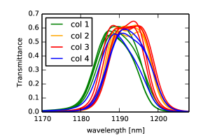
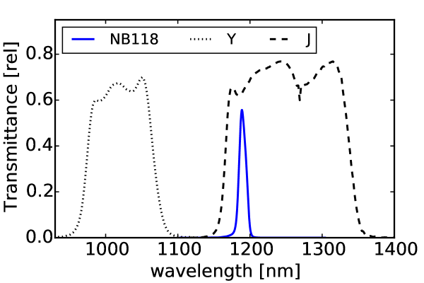
Throughout this paper our results were based on the set of VISTA NB118 filters. In Fig. 19 we show all 16 filter curves used in this study and in Fig. 20 one of the filters (filter 15) is shown in comparison to the Y and J filters.
So far, we neglected the uncertainties in the measured filter curves. Unfortunately, there are several sources of potentially significant errors in the available filter curves. We therefore summarize in this appendix the origin of the assumed filter curves and our current understanding of their accuracy.
The VIRCAM filter curves are based on laboratory scans carried out at room temperature in the normal incidence collimated beam. These measurements have been supplied by the filter manufacturer, NDC 252525NDC Infrared Engineering; http://www.ndcinfrared.com.
However, as the NB118 filters are multilayer dielectric interference filters, the transmittance curves depend both on the temperature and the angle of incidence of the beam. Qualitatively, both a cooling and the change from the collimated beam to larger incidence angles lead to a shift of the passband towards shorter wavelengths (Morelli 1991). This is relevant, as in VIRCAM the filters are located in a fast convergent beam (e.g. Atad-Ettedgui & Worswick 2003) at cryogenic temperatures. The convergent beam can be understood as formed by rays coming from different incidence angles, each of which sees a filter curve corresponding to its incidence angle.
One way to approximate the actual filter curves within the cryogenic convergent beam is to do an entirely theoretical conversion from the collimated beam measurement. Assuming a temperature dependence of (NDC), the difference of 205K between room temperature and filter temperature in VIRCAM (; private communication ESO), equals a blueward shift of 4.26nm. We made the assumption that the shape of the transmittance curve is preserved under the temperature shift. The justification of this assumption was confirmed by a re-measurement of a witness sample done by NDC in 2013.
The transformation between collimated and convergent beam was based on the assumption that it is possible to approximate the filter curve in a collimated beam with non-normal incidence angle from that for normal incidence by:
| (20) |
As the range of relevant incidence angles in the VISTA beam extents up to , eq. 20 must be a good approximation for a large range of angles. According to Morelli (1991) a conservation of the general filter curve shape is a good approximation up to angles of . In the literature exist a few examples, where measurements of similar NIR filters have been published for different incidence angles. For some of them the results seem approximately consistent with eq. 20 (e.g. Ghinassi et al. 2002), while there is for others a stronger discrepancy (e.g Vanzi et al. 1998). Again based on a witness-sample, NDC provided us with measurements of the material for incidence angles up to . The shape was indeed approximately conserved.
VISTA’s beam can be characterized by the radiant intensity as a function of the angle of incidence, . Here, and are the two dimensional polar-coordinates characterizing the latter. Neglecting all effects of wave optics, can be described to first order by an annulus with constant value. The annulus’s inner radius and outer radius have values of and , respectively (Nilsson et al. 2007). This annulus is shifted corresponding to the object’s position in the field of view in the , plane. The angle of incidence of the annulus’s center is related to the object’s position on the sky by (Findlay 2012). The position is stated here in percentages of detectors.
With this input, the effective filter curve for the complete beam can be calculated by (e.g. Lissberger 1970):
| (21) |
Consequently, we can finally estimate the shape of the filter curves in VIRCAM’s convergent beam by combining equations 20 and 21.
| (22) |
We tested our script doing the actual convergent beam conversion based on a 1% top-hat filter and comparing the results to those presented in Bland-Hawthorn et al. (2001).
Filter curves for the different steps in the conversion were shown in Fig. 4 of Milvang-Jensen et al. (2013). Milvang-Jensen et al. (2013) found an unexpected shift of the filter curves towards the red by about . While we are still investigating possible physical reasons for the shift, we assume in this work the predicted convergent beam curves shifted by towards the red to account for this finding. The fact that the presented TPV method works well for the actual data under this assumption, further indicates that these filter curves are a reasonable assumption.
Appendix B Quantitative assessment of throughput variation for all possible NB118 pairs
The suitability of a filter combination for the TPV can be assessed through - curves, as discussed in sec. 2.2. We characterized the - curves for all 120 possible VIRCAM NB118 combinations by following three quantities:
-
•
Difference between maximum and minimum
-
•
Percentage of the wavelength range, where the values are unique
-
•
Average absolute slope () and its standard deviation
For the calculation of these values a relevant wavelength interval needs to be chosen. We assumed the wavelength range, where the transmittance of the combined effective filter is not below 2/30 of its maximum value. This threshold is a reasonable number, as it approximately corresponds to the ratio between the FWHMs of the NB118 filters and J. Consequently, an emission line causes a stronger excess in the NB118 filters than in J within the included range.
The resulting values for all 120 combinations are listed in Table 5. For the example filter-combination 14 & 15, as shown in Fig. 1, the range in values is 3.12 with a uniqueness of 100%. The average absolute slope is . The assumed wavelength interval, as defined above, is indicated in the left panel of Fig. 1. Assuming e.g. 5 detections in each of the two filters, corresponding to an error of for the magnitude difference, this would allow on average for a very good wavelength resolution of about .
| 1 | 2 | 3 | 4 | 5 | 6 | 7 | 8 | 9 | 10 | 11 | 12 | 13 | 14 | 15 | 16 | |
|---|---|---|---|---|---|---|---|---|---|---|---|---|---|---|---|---|
| 1 | 0.070.05 | 0.060.06 | 0.040.03 | 0.150.09 | 0.120.09 | 0.130.10 | 0.130.07 | 0.160.09 | 0.080.07 | 0.090.08 | 0.140.08 | 0.130.06 | 0.140.08 | 0.030.01 | 0.160.10 | |
| 2 | 77./ 1.39 | 0.010.00 | 0.050.03 | 0.210.12 | 0.180.11 | 0.190.13 | 0.200.10 | 0.210.12 | 0.120.08 | 0.140.09 | 0.200.11 | 0.190.09 | 0.190.11 | 0.070.05 | 0.220.13 | |
| 3 | 71./ 1.30 | 40./ 0.20 | 0.050.03 | 0.210.12 | 0.180.12 | 0.190.13 | 0.190.10 | 0.210.12 | 0.110.08 | 0.140.08 | 0.200.11 | 0.190.09 | 0.190.11 | 0.070.05 | 0.220.13 | |
| 4 | 17./ 0.57 | 95./ 1.05 | 72./ 0.92 | 0.180.11 | 0.150.11 | 0.170.12 | 0.160.09 | 0.190.11 | 0.090.08 | 0.110.09 | 0.170.10 | 0.150.09 | 0.160.10 | 0.060.04 | 0.190.12 | |
| 5 | 90./ 3.36 | 83./ 4.71 | 86./ 4.64 | 82./ 3.86 | 0.040.03 | 0.040.03 | 0.030.02 | 0.030.02 | 0.120.08 | 0.090.06 | 0.010.01 | 0.060.04 | 0.040.03 | 0.160.07 | 0.080.06 | |
| 6 | 82./ 2.52 | 76./ 3.88 | 80./ 3.81 | 63./ 3.05 | 48./ 0.69 | 0.020.01 | 0.040.02 | 0.050.04 | 0.090.06 | 0.060.04 | 0.030.03 | 0.080.05 | 0.070.04 | 0.120.08 | 0.100.08 | |
| 7 | 79./ 2.74 | 73./ 4.10 | 77./ 4.04 | 59./ 3.27 | 29./ 0.43 | 28./ 0.26 | 0.040.02 | 0.050.04 | 0.110.08 | 0.080.05 | 0.030.02 | 0.080.05 | 0.070.04 | 0.130.09 | 0.100.07 | |
| 8 | 82./ 2.79 | 78./ 4.16 | 81./ 4.08 | 77./ 3.32 | 68./ 0.56 | 2./ 0.34 | 0./ 0.25 | 0.040.03 | 0.100.08 | 0.070.06 | 0.020.01 | 0.050.04 | 0.040.04 | 0.130.06 | 0.080.08 | |
| 9 | 86./ 3.44 | 75./ 4.76 | 79./ 4.72 | 77./ 3.95 | 37./ 0.42 | 50./ 0.98 | 48./ 0.80 | 81./ 0.85 | 0.130.10 | 0.100.08 | 0.030.02 | 0.050.04 | 0.040.02 | 0.160.07 | 0.060.05 | |
| 10 | 27./ 1.30 | 83./ 2.38 | 92./ 2.28 | 43./ 1.56 | 81./ 2.37 | 55./ 1.68 | 51./ 1.93 | 55./ 1.85 | 65./ 2.60 | 0.040.02 | 0.110.08 | 0.100.09 | 0.110.10 | 0.080.05 | 0.150.12 | |
| 11 | 53./ 1.74 | 78./ 2.97 | 87./ 2.89 | 71./ 2.16 | 68./ 1.69 | 45./ 1.00 | 43./ 1.25 | 42./ 1.18 | 58./ 1.93 | 78./ 0.68 | 0.080.06 | 0.090.08 | 0.090.08 | 0.090.06 | 0.130.11 | |
| 12 | 87./ 3.09 | 81./ 4.45 | 84./ 4.38 | 79./ 3.61 | 37./ 0.20 | 30./ 0.50 | 20./ 0.35 | 46./ 0.36 | 79./ 0.53 | 69./ 2.14 | 65./ 1.48 | 0.050.03 | 0.040.02 | 0.150.06 | 0.080.06 | |
| 13 | 99./ 2.96 | 93./ 4.29 | 95./ 4.20 | 90./ 3.35 | 22./ 0.81 | 5./ 0.58 | 3./ 0.61 | 1./ 0.46 | 42./ 0.87 | 44./ 1.88 | 24./ 1.31 | 18./ 0.61 | 0.020.02 | 0.140.05 | 0.060.04 | |
| 14 | 93./ 3.04 | 83./ 4.38 | 86./ 4.31 | 83./ 3.53 | 16./ 0.59 | 17./ 0.64 | 13./ 0.55 | 16./ 0.54 | 52./ 0.62 | 53./ 2.05 | 35./ 1.42 | 9./ 0.39 | 28./ 0.31 | 0.140.06 | 0.050.04 | |
| 15 | 6./ 0.25 | 57./ 1.37 | 48./ 1.29 | 8./ 0.56 | 100./ 3.41 | 91./ 2.55 | 88./ 2.77 | 93./ 2.82 | 92./ 3.49 | 41./ 1.25 | 66./ 1.69 | 100./ 3.14 | 99./ 3.00 | 100./ 3.12 | 0.170.09 | |
| 16 | 91./ 3.70 | 84./ 4.99 | 86./ 4.95 | 84./ 4.17 | 12./ 0.79 | 15./ 1.24 | 14./ 1.08 | 19./ 1.01 | 3./ 0.55 | 50./ 2.76 | 39./ 2.10 | 12./ 0.80 | 44./ 1.01 | 32./ 0.71 | 98./ 3.77 |
Appendix C Expected number of emitters in regions of filter overlap
C.1 Simulation
We estimated the number of emitters expected to be found in the field covered by two differing filters as a function of line flux both for the DR2 and the finalized UltraVISTA. For this purpose we created 300000 simulated objects with a continuum flat in , a fixed [N ii] ratio of either or , a random central wavelength between , and assigned to each of these objects the same fixed input line luminosity, . The were drawn from a log-normal distribution with a and . These values were taken from the best fit distribution obtained by Ly et al. (2011) based on NEWFIRM narrowband observations at a similar wavelength as the UltraVISTA NB118 filters.
After assigning to these 300000 objects random positions within a field, we determined for each of the jitter positions in each of the three pawprints in the UltraVISTA NB118 observing pattern, whether an object is observed and if yes, in which filter. For computational reasons, we only did 28 random jitters per pawprint drawn from a 2”x 2” box.
In each of the individual simulated pointings we determined for each object falling within the boundaries corresponding to a filter the synthetic (eq. 2) and the corresponding error on the , which we separated into and for object and background, respectively.262626As the considered observations are background-limited, we could in principle ignore . We kept it for generality of our simulator. The calculations were based on the same ZPs, gains, and detector-depended sky-counts, and observation times for the DR2 and final UltraVISTA, as described in sec. 4.3. Finally, we combined for each of the individual pawprints the signal from the different jitter positions by weighting with and propagated the errors on the noise. This simulated observing and stacking strategy resembles that for the actual UltraVISTA observations.
C.2 Method
As the measured source flux density scales for fixed linearly with line luminosity both for the NB and the BB filter, we can based on , , obtained for the input line luminosity, , directly determine for a chosen color-significance the required to fulfill the inequality 9. This is to solve a quadratic equation in the common way, where , , and are given as:272727For the strongly background limited UltraVISTA observations, the inclusion of the source noise is in principle not necessary and is only included for generality.
| (23) | |||||
| (24) | |||||
| (25) |
is the ratio between and . Similarly, we can determine the factor , required to fulfill eq. 10. Having determined the factors and for each of the two contributing filters, we find the minimum factor , which fulfills the color-significance combined with the color-cut in one of the two filters and the detection significance in the other filter. If any of the criteria is not fulfilled at any flux, we set to . We also applied the same region mask as used for the actual data (cf. eq. 11).
Based on the ’s obtained for each simulated object, we directly determined the fraction of input objects being detected as a function of line luminosity. Eventually, multiplying this luminosity completeness function with luminosity functions from the literature and the volume covered by the random box allowed for an estimate of the number of objects expected to be detected as a function of line luminosity. This takes fully account for the filter curve shapes and the different background brightnesses in the individual filters.
We used the Schechter (1976) parameterizations of the three LFs stated by Ly et al. (2011), including their own and the two LFs of Villar et al. (2008) and Sobral et al. (2009). The LFs stated in Ly et al. (2011) are reddening and completeness corrected. As we need for the purpose of our simulation non-reddening corrected LFs, we convert their Schechter LFs to reddened LFs, by inverting the same SFR depended correction as used in Ly et al. (2011), which is based on Hopkins et al. (2001).282828There are small differences in the two versions, as mentioned in Ly et al. (2007). Assuming the underlying direct proportionality between SFR and H luminosity (Kennicutt 1998), the relation between intrinsic, , and observed luminosity, , can be written as (Ly et al. 2011):
| (27) |
C.3 Results
The number of galaxies expected to be selected per unit logarithmic interval by the criteria stated in eq. 7–11 are shown in Fig. 21 for the three different LFs. For the Ly et al. (2011) LF, the result is shown in addition to assuming also for the assumption of . For orientation, luminosities corresponding to fluxes of approximately , , , and are marked with small arrows.292929Approximately, as the actual ratio between line flux and line luminosity depends on the luminosity distance, which slightly varies over the considered wavelength range.
Integrated numbers within the 12 patches with contribution of two different filters are stated down to the detection limit and to the four reference fluxes in Table 6. Already in the DR2, we would expect to have on the order of 200 emitters in the patches of overlapping filters. The total UltraVISTA field is expected to have about three times the numbers stated in Table 6 and the number in the final UltraVISTA data will almost double the number compared to the DR2.
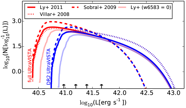
| flux [] | |||||
|---|---|---|---|---|---|
| LF | all | ||||
| UltraVISTA DR2 | |||||
| LY11 | 184 (113) | 169 (113) | 119 (90) | 77 (60) | 39 (30) |
| SO09 | 250 (165) | 237 (164) | 184 (140) | 132 (102) | 76 (59) |
| VI08 | 275 (156) | 246 (155) | 150 (113) | 79 (61) | 25 (19) |
| Full UltraVISTA | |||||
| LY11 | 373 (235) | 198 (154) | 126 (98) | 79 (62) | 39 (30) |
| SO09 | 413 (280) | 268 (209) | 192 (150) | 135 (106) | 76 (60) |
| VI08 | 666 (400) | 299 (233) | 161 (126) | 81 (64) | 25 (19) |
Appendix D Expected line S/N in NB and BB filters
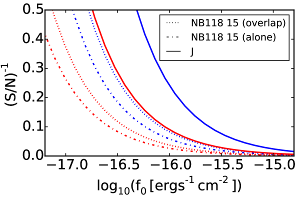
Fig. 22 shows the inverse of the that an emission line point source with infinite would reach for a given line flux in J and NB118, respectively, both for the UltraVISTA DR2 and the expected full UltraVISTA. The calculation was based on eq. 6 and the simulation inputs described in sec. 4.1. Assuming that the continuum flux density could be estimated without uncertainty, these would be the S/N values for the line alone, independent of the EW.
NB118 results are shown for the peak of filter 15, which has a typical sky-brightness, and are plotted both for the typical per-pixel integration time and half its value. The latter would be applicable when sharing the available time equally between two contributing filters.
Even so the UltraVISTA BB data is extremely deep, the line S/N in the NB118 is a factor 4.1 or 3.4 higher than that in J, for the DR2 and the expected final survey data respectively. On the other hand, at low transmittances of the NB filters, the line S/N in J becomes equivalent or even higher than that in the NB filter.
Appendix E Full SED fitting results
The full results from the SED fitting for the sample of NB excess objects with observations available in either of the NB118 pairs 9 & 10, 14 & 15, or 15 & 16, as described in sec. 5.6.1, are listed in Table 7. Additionally, the table includes the estimated through the TPV.
| SED Fitting | TPV | ||||||||||
|---|---|---|---|---|---|---|---|---|---|---|---|
| IDa𝑎aa𝑎aNBES | RA (J200) | DEC (J2000) | Massb𝑏bb𝑏b; mass in stars at time of observation | c𝑐cc𝑐cAssuming Calzetti et al. (2000) extinction law | d𝑑dd𝑑d | e𝑒ee𝑒e | f𝑓ff𝑓fredshifts from Ilbert et al. (2013) | g𝑔gg𝑔g; SFR averaged over before time of observation | hℎhhℎhzCOSMOS confidence class 13.5 (BL AGN) | i𝑖ii𝑖iCovering fraction of the gas; related to the escape of ionizing radiation through | j𝑗jj𝑗j |
| 7 | +10:01:54.356 | +01:53:18.36 | |||||||||
| 14 | +10:01:57.962 | +01:53:57.58 | |||||||||
| 33 | +10:01:45.444 | +01:55:22.99 | |||||||||
| 94 | +10:01:37.653 | +02:10:33.39 | |||||||||
| 96 | +10:02:12.744 | +02:10:47.98 | |||||||||
| 97 | +10:02:16.988 | +02:10:55.96 | |||||||||
| 99 | +10:02:15.195 | +02:10:54.36 | |||||||||
| 104 | +10:02:15.978 | +02:11:18.89 | |||||||||
| 105 | +10:02:07.660 | +02:11:20.09 | |||||||||
| 111 | +10:02:16.354 | +02:12:00.30 | |||||||||
| 113 | +10:01:41.651 | +02:12:02.75 | |||||||||
| 114 | +10:02:09.637 | +02:12:02.47 | |||||||||
| 117 | +10:02:17.543 | +02:12:12.54 | |||||||||
| 121 | +10:02:03.952 | +02:12:39.54 | |||||||||
| 122 | +10:02:01.838 | +02:12:38.81 | |||||||||
| 124 | +10:02:16.714 | +02:12:55.00 | |||||||||
| 125 | +10:02:18.112 | +02:13:02.53 | |||||||||
| 126 | +10:01:47.095 | +02:13:26.64 | |||||||||
| 128 | +10:01:46.900 | +02:13:30.85 | |||||||||
| 131 | +10:02:06.263 | +02:13:40.26 | |||||||||
| 135 | +10:01:52.737 | +02:13:53.75 | |||||||||
| 138 | +10:02:17.661 | +02:14:02.29 | |||||||||
| 147 | +10:01:46.836 | +02:14:24.08 | |||||||||
| 150 | +10:02:12.970 | +02:14:28.42 | |||||||||
| 153 | +10:02:18.594 | +02:14:41.36 | |||||||||
| 161 | +10:01:54.279 | +02:15:26.80 | |||||||||
| 164 | +10:02:04.380 | +02:15:30.63 | |||||||||
| 167 | +10:01:53.203 | +02:15:49.45 | |||||||||
| 170 | +10:02:15.102 | +02:15:59.41 | |||||||||
| 172 | +10:00:46.944 | +02:26:10.89 | |||||||||
| 186 | +10:00:12.440 | +02:27:46.31 | |||||||||
| 204 | +10:00:41.641 | +02:29:02.47 | |||||||||
| 205 | +10:00:41.331 | +02:29:04.57 | |||||||||
| 226 | +10:00:36.526 | +02:31:07.13 | |||||||||
| 235 | +10:00:44.244 | +02:32:18.36 | |||||||||
Appendix F Details about the selection of NB excess objects
F.1 Color correction for J band magnitudes
The NB118 filter is at the blue end of the J passband (Fig. 20). Consequently, an estimate of the continuum at the wavelength of the NB118 filter needs to include more information than alone, as it is necessary to correct for the galaxies’ intrinsic colors.
Therefore, we estimated the continuum magnitude at the wavelength of the NB118 filter, , through a linear combination of Y and J. While this approach is identical to Milvang-Jensen et al. (2013), we adjusted the exact linear combination for two reasons: The zeropoints for the broadband data have been adjusted between the UltraVISTA DR1 (McCracken et al. 2012), which was used by them, and the DR299footnotemark: 9 used by us. Further, we applied in this work corrections between the Vega magnitude system and the AB system, which differ slightly from those used for both UltraVISTA data releases and the work of Milvang-Jensen et al. (2013). In the following, we justify the chosen color correction.
Under the assumption that SEDs are power laws over the wavelength range covered by the Y and J filters, the appropriate combination can be determined based on the filters’ central wavelengths. This results in:
| (28) |
This corresponds to eq. 14, when using flux densities instead of magnitudes.
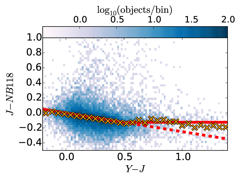
The validity of eq. 28 can be verified empirically. Due to the simplicity of a one-color correction, this can be easily visualized. In Fig. 23 we show the 2d histogram of the number of objects with as a function of . All sources from the NB118 detected catalog which have a NB118 detection above , and at least detections in and , are included. It is clear that the locus of the objects follows the line very well for . This confirms empirically that the relation is justified.
The number of objects is small for . Nevertheless, it can be concluded that the line with a slope of -0.25 is not a good representation of their typical colors. The main reason is that this part of the color space is mainly populated by passive galaxies at . Their red colors are not caused by dust but by the Balmer/ break located at the interface of Y and J. While there might be some identifiable trend in as a function of also beyond , the number of objects is small, and we decided to follow also in this part of the color space Milvang-Jensen et al. (2013). They used for the reddest objects a constant correction to . We have determined this constant correction as minus the median color of all objects with and derived a value of 0.126. In order to have a continuous transition from 28 into the constant part, we use:
| (29) |
Expressed as flux densities, this is equivalent to eq. 13.
Formally, we set in absence of a Y detection () simply to . However, this is not really relevant, as we do not have any NB excess objects without Y detection in the NB118 catalog created with the conservative SExtractor parameters (cf. sec. F.2) used for this work.
F.2 Narrowband excess and detection thresholds
When selecting emission line galaxies from NB data, thresholds for the magnitude excess (cf. eq. 8) and its significance need to be set (cf. eq. 9). Good selection criteria provide a compromise between the inclusion of low emitters and a small contamination from objects without emission line in the NB filter.
Milvang-Jensen et al. (2013) concluded based on an analysis of stellar population models that , which is for power law SEDs expected to be close to zero, does also for realistic stellar SEDs not exceed 0.2 by much. The largest deviations from zero are expected at redshifts where the /Balmer break and strong absorption lines fall into the wavelength range of the Y and J filters, especially at population ages where these features are pronounced.313131Even larger deviations are theoretically possible for galaxies with , where the Lyman break would be in this range. A selection threshold of can be considered as a conservative choice to identify emission line galaxies. corresponds to an of .323232Averaged over all 16 filters, assuming emission lines at the wavelengths corresponding to the peak of the respective filters and assuming a continuum flat in .
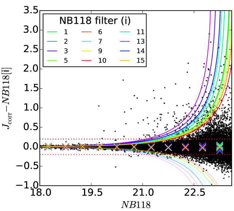
The required color combined with a significant color excess (eq. 9) is expected to result in a nearly pure sample of NB excess objects. We demonstrate this in Fig. 24, where data for one filter from each of the 12 regions with overlapping filters is included. The plot shows 12 different lines for the color-excess criterion (eq. 9). The reason for this is that the depth in the 12 relevant filters strongly differs. In addition to the relevant selection curves, we also show these curves mirrored at . This allows, at least to some extent, to judge the contamination fraction due to statistical noise. It is as expected very low.
It is noteworthy that these conservative selection criteria will miss [O ii] emitters at (cf. also Milvang-Jensen et al. 2013). However, this is no problem for the present work, as we are here not interested in [O ii] emitters. Refined selection criteria for these objects will be discussed in a forthcoming work.
In addition to the criteria described above, we decided to use a relatively high detection and analysis threshold of in a least four neighboring pixels for SExtractor. This detection threshold is at the limit of affecting the completeness within our selection criteria: A lower detection threshold would slightly increase the number of objects in the NBES. E.g. at a very low threshold of , the NBES sample would include 13 more objects (252 vs 239). Nevertheless, we decided to use the catalog, as we aimed in this work to include only clean and well centered detections.