Solar energy production:
Short-term forecasting
and risk management

Abstract

Electricity production via solar energy is tackled via short-term forecasts and risk management. Our main tool is a new setting on time series. It allows the definition of “confidence bands” where the Gaussian assumption, which is not satisfied by our concrete data, may be abandoned. Those bands are quite convenient and easily implementable. Numerous computer simulations are presented.

1 Introduction

1.1 Generalities

The following lines by Reikard (2009) provide an excellent introduction to our subject: The increasing use of solar power as a source of electricity has led to increased interest in forecasting radiation over short time horizons. Short-term forecasts are needed for operational planning, switching sources, programming backup, and short-term power purchases, as well as for planning for reserve usage, and peak load matching. There are many approaches as summarized by Trapero, Kourentzes & Martin (2015): The diversity of solar radiation forecasting methodologies can be classified according to the input data and the objective forecasting horizon. For instance, NWP (Numerical Weather Prediction) models, which are based on physical laws of motion and conservation of energy that govern the atmospheric air flow, are operationally used to forecast the evolution of the atmosphere from about 6 h onward. Although NWP models are powerful tools to forecast solar radiation at places where ground data are not available, many near-surface physical processes occur within a single grid box and are too complex to be represented and solved by equations. Thus, NWP models cannot successfully resolve local processes smaller than the model resolution. Satellite-derived solar radiation images are a useful tool for quantifying solar irradiation at ground surface for large areas, but they need to set an accurate radiance value under clear sky conditions and under dense cloudiness from every pixel and every image …These limitations have placed time series analysis as the dominant methodology for short-term forecasting horizons from 5 min up to 6 h. See Kleissl (2013) for a slightly different standpoint.

Diverse viewpoints on time series have of course been employed. See, e.g., Bacher, Madsen & Nielsen (2009); Diagne, David, Lauret, Boland & Schmutz (2013); Duchon & Hale (2012); Lauret, Voyant, Soubdhari, David & Poggi (2015); Martín, Zarzalejo, Polo, Navarro, Marchante & Cony (2010); Reikard (2009); Trapero, Kourentzes & Martin (2015); Voyant, Muselli & Nivet (2011); Voyant, Paoli, Muselli & Nivet (2013); Voyant, Soubdhan, Lauret, David & Muselli (2015); Yang, Sharma, Ye, Lim, Zhao & Aryaputer (2015), and the references therein. We follow here another model-free setting (Fliess & Join (2009, 2015a, 2015b); Fliess, Join & Hatt (2011a, b)). With respect to solar energy production they have already been compared to techniques stemming especially from persistence and from artificial neural nets by Join, Voyant, Fliess, Nivet, Muselli, Paoli & Chaxel (2014) and by Voyant, Join, Fliess, Nivet, Muselli & Paoli (2015). Let us emphasize that our techniques are quite far from today’s dominant viewpoint on time series (see, e.g., Meuriot (2012) and the references therein).

1.2 Forecasting and risk

According to a theorem due to Cartier & Perrin (1995) the following additive decomposition holds for any time series $X$ under quite weak assumptions:

$$\boxed{X(t)=E(X)(t)+X_{\tiny{\rm fluctuation}}(t)}$$ (1)

where

• the mean, or average, or trend, $E(X)(t)$ is quite smooth,

• $X_{\tiny{\rm fluctuation}}(t)$ is quickly fluctuating.

The decomposition (1) is unique up to a “small” additive quantity. Our short-term forecast techniques are based on a local mathematical analysis of $E(X)(t)$ (Fliess & Join (2009); Fliess, Join & Hatt (2011b)), which is inspired by recent advances in the field of estimation. They yield good results and are quite easy to implement. Their application to solar energy by Join, Voyant, Fliess, Nivet, Muselli, Paoli & Chaxel (2014) and by Voyant, Join, Fliess, Nivet, Muselli & Paoli (2015) do not necessitate contrarily to most other approaches big data, i.e., large historical data. Any type of forecast is always approximate. Here, according to Formula (1), the quick fluctuations $X_{\tiny{\rm fluctuation}}(t)$ explain to a large extent this discrepancy. This inherent risk does not seem to have been seriously investigated in the literature on solar energy although it plays obviously a key rôle in the energy production. We follow (Abouaïssa, Fliess & Join (2016)) and exploit the viewpoint on volatility developed by Fliess, Join & Hatt (2011a, b). Classic normality tests show that our concrete time series are not related to Gaussian processes. We replace therefore the well known confidence intervals, which do not make much sense in this situation, by the confidence bands which bear some similarity with the famous Bollinger bands in technical analysis (Bollinger (2001)).This might be an important advance in risk analysis.

Remark 1

See, e.g., Willink (2013) for a most rewarding account on confidence intervals.

1.3 Organization of the paper

The paper by Abouaïssa, Fliess & Join (2016) in this conference already presents a summary of our approach to time series. Therefore this material will not be repeated here. It gives more room to Section 2 where

• a type of volatility is considered,

• confidence bands are defined,

• we report quite numerous numerical experiments which are based on real meteorological data.

Some thoughts about solar energy forecasting and risk management are discussed in Section 3.

2 Numerical experiments

2.1 Presentation

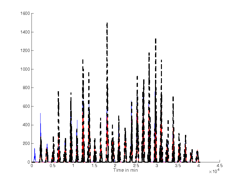
Write $X(t)$ the solar irradiance at time $t$. Those data are given by measurements every minute in Nancy, France, during the year 2013. In order to simplify the presentation of our computer calculations, we only utilize here the months of February and June.

Write $X_{\text{pred$60$}}(t)$ the forecast 1 h ahead of $X(t)$ as obtained by Join, Voyant, Fliess, Nivet, Muselli, Paoli & Chaxel (2014). The results in Figures 2 and 6 are borrowed from the same reference.

2.2 Volatility

Define the volatility via

$$\text{{\bf Vol}}(t)=|X(t)-X_{\text{pred$60$}}(t-60)|$$ (2)

where $X_{\text{pred$60$}}(t-60)$ is the forecast 1 h ahead of $X(t-60)$. As stated before, it is obtained via the mean $E(X)(t)$ (see Equation (1)). Figures 3 and 7 display the results. For simplicity’s sake, set the following elementary persistence scheme for volatility

$$\text{{\bf Vol}}_{\text{pred$60$}}(t)=\text{{\bf Vol}}(t)$$

where $\text{{\bf Vol}}_{\text{pred$60$}}(t)$ is the forecast 1 h ahead of $\text{{\bf Vol}}(t)$.

2.3 Normality tests

Let us associate to Equation (2) the Equation

$$\text{Diff}(t)=X(t)-X_{\text{pred$60$}}(t-60)$$

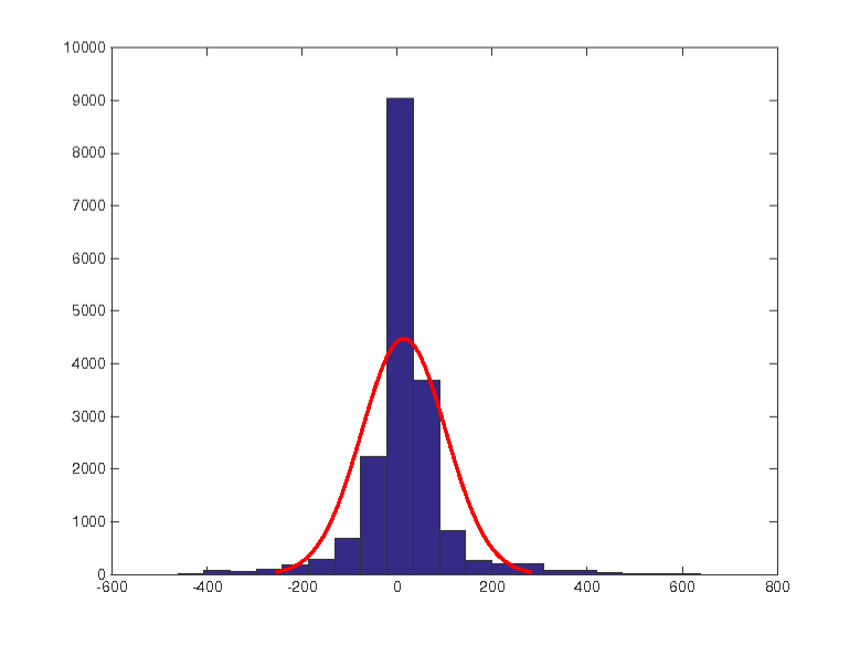
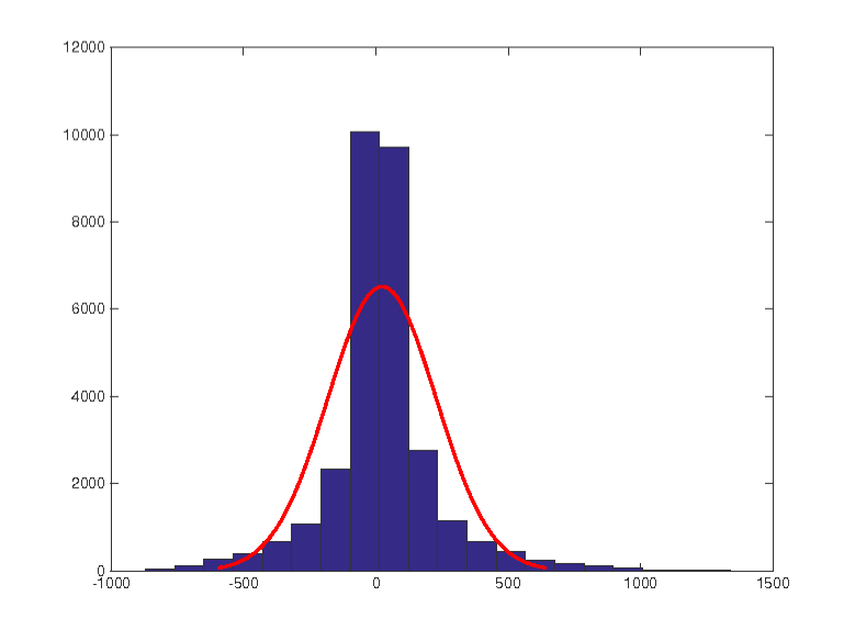
Three classic normality tests (see, e.g., Bourbonnais & Terraza (2010); Cryer & Chan (2008); Jarque & Bera (1987); Judge, Griffiths, Hill, Lütkepol & Lee (1988); Thode (2002)), namely

• Jarque-Bera,

• Kolmogorov-Smirnov,

• Lilliefors,

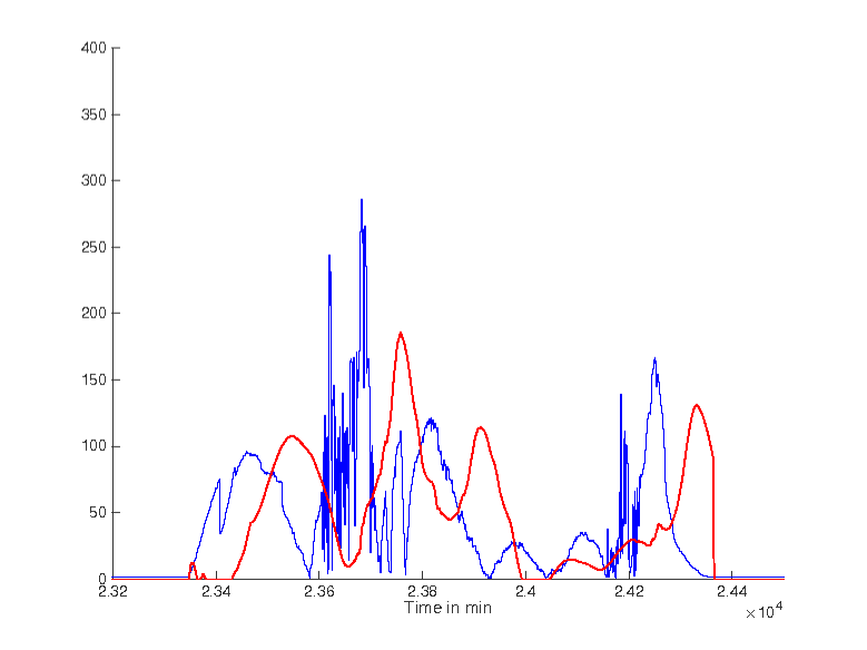
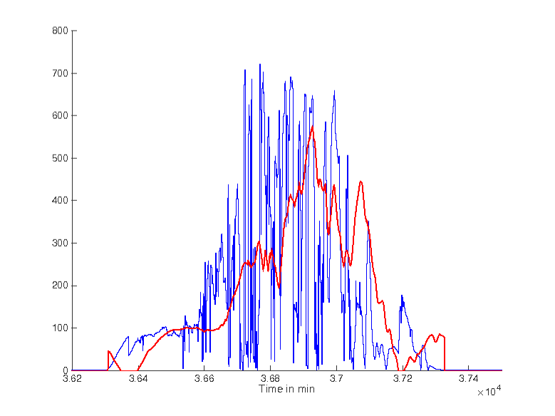
reject the Gaussian property of the signal $\text{Diff}(t)$ for the twelve months of 2013. This is illustrated by Figures 1-(a) and 1-(b).

(a) February

(b) June

Figure 1: Signal distribution (blue) and the Gaussian distribution (red)

2.4 Towards confidence bands

Define a first confidence band $\text{\bf CB}_{1,\ \text{pred$60$}}(t)$ by its frontiers

$$X_{\text{pred$60$}}(t)\pm\text{{\bf Vol}}_{\text{pred$60$}}(t)$$

See Figures 4 and 8.

In order to improve $\text{\bf CB}_{1,\ \text{pred$60$}}(t)$, define $\text{\bf CB}_{2,\ \text{pred$60$}}(t)$ by new frontiers

$$X_{\text{pred$60$}}(t)\pm\alpha\text{{\bf Vol}}_{\text{pred$60$}}(t)$$

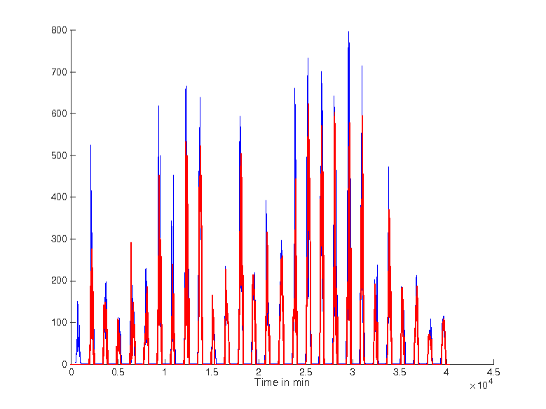
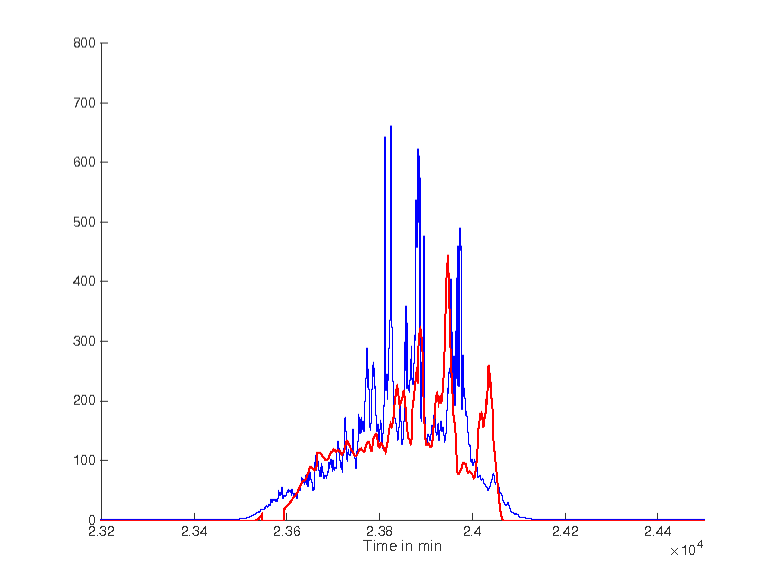
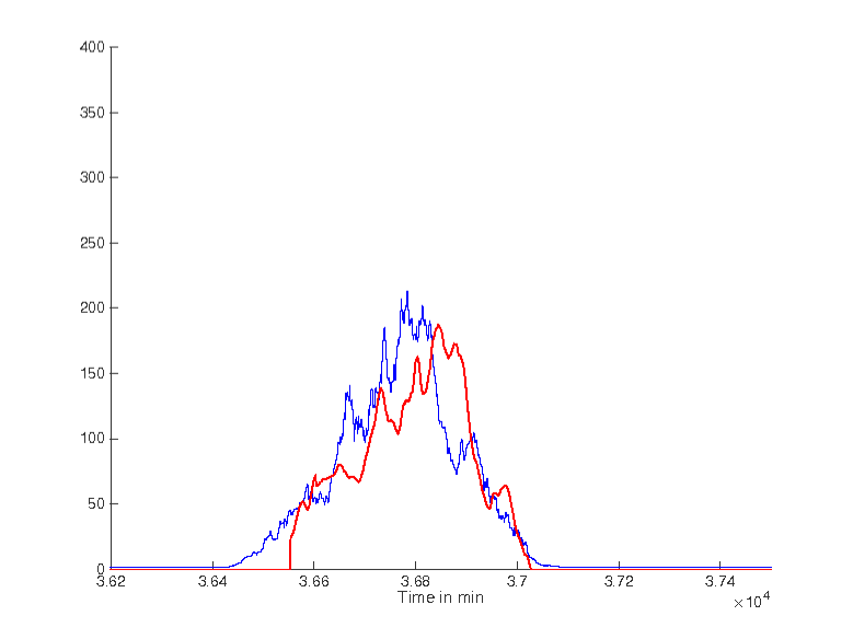
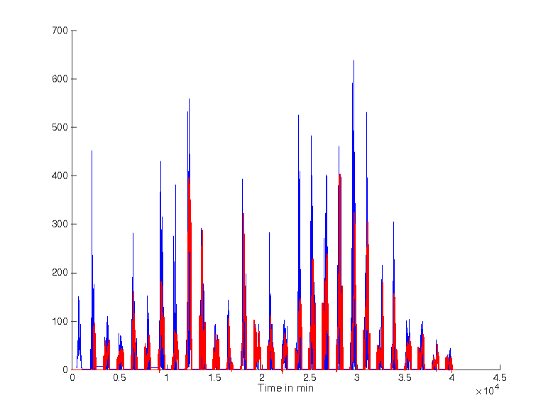
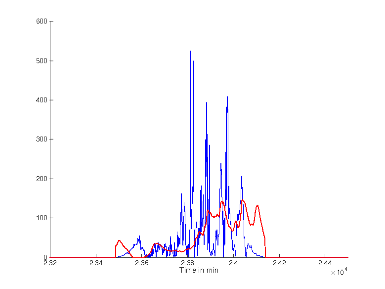
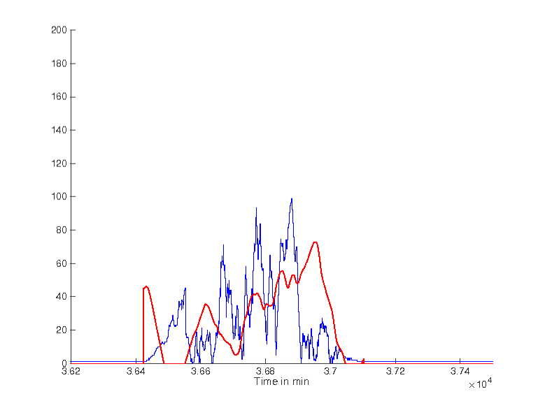
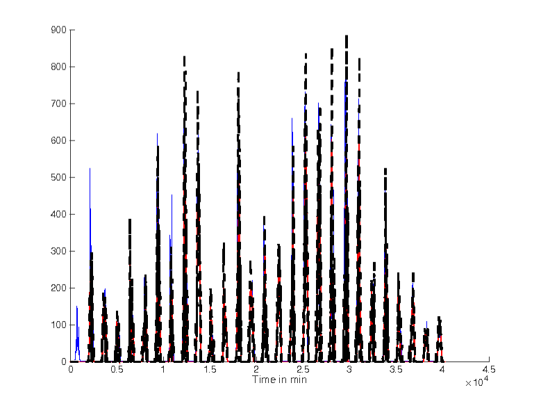
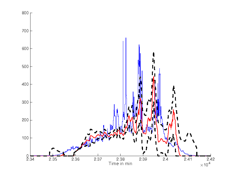
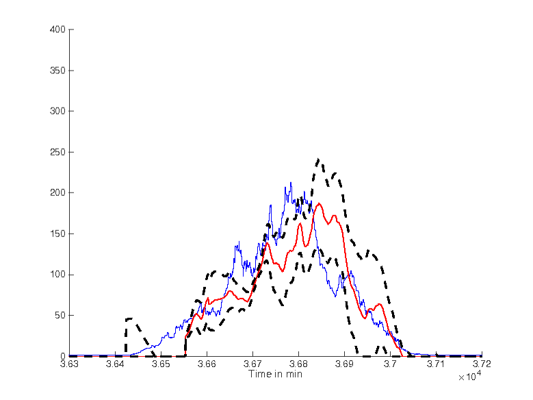
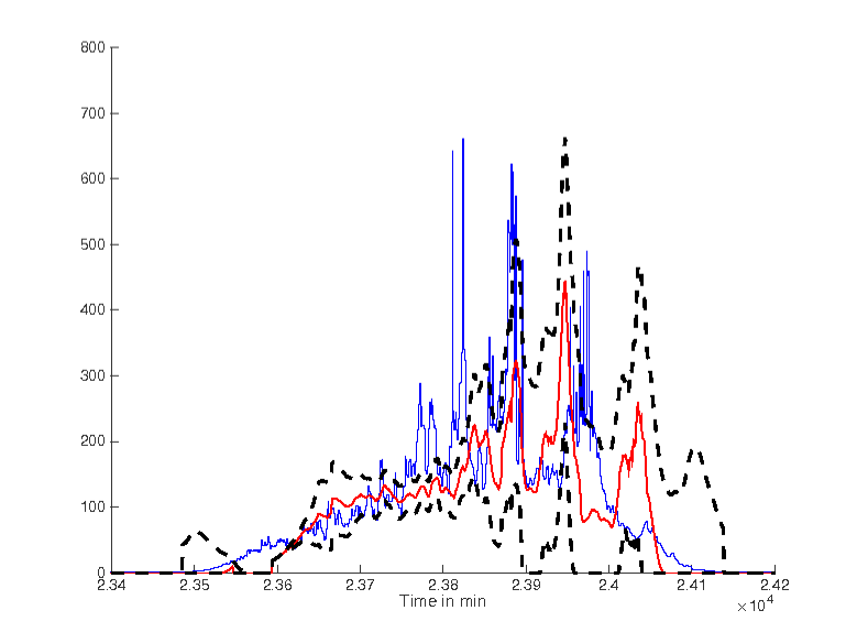
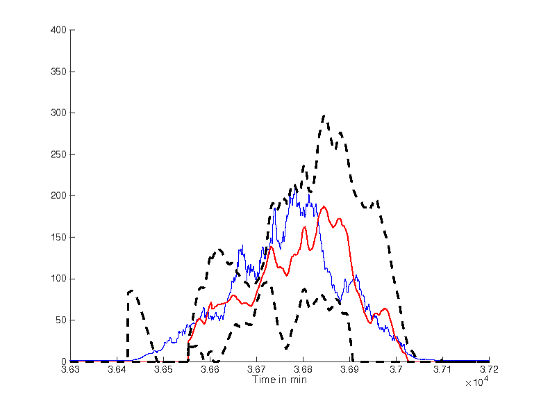
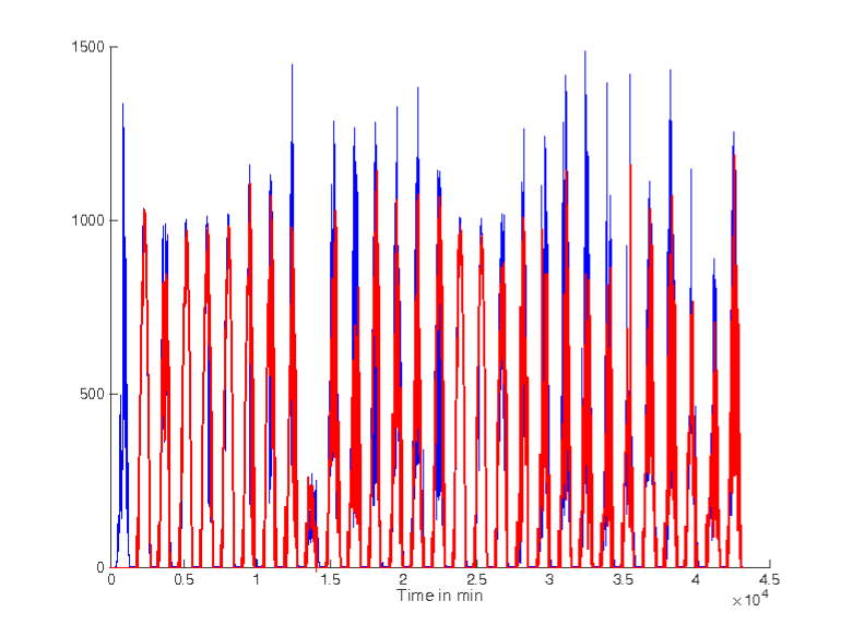
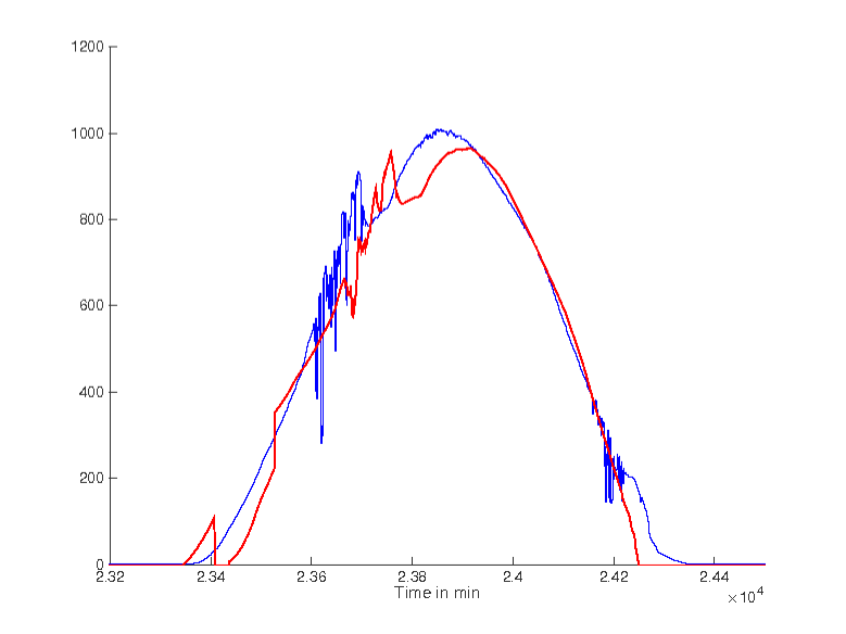
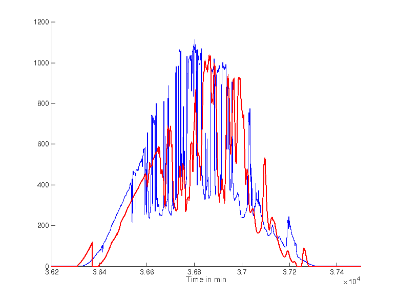
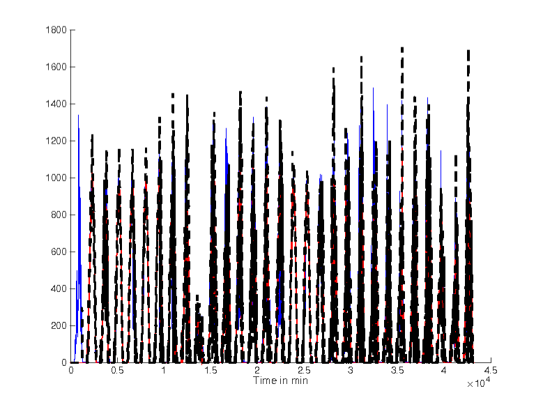
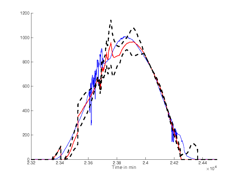
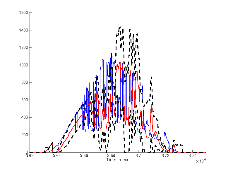
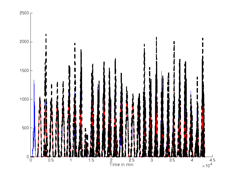
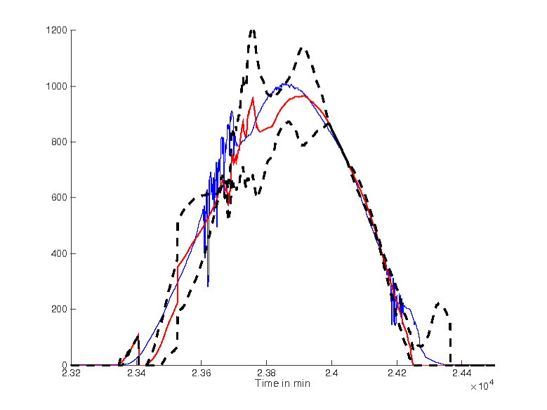
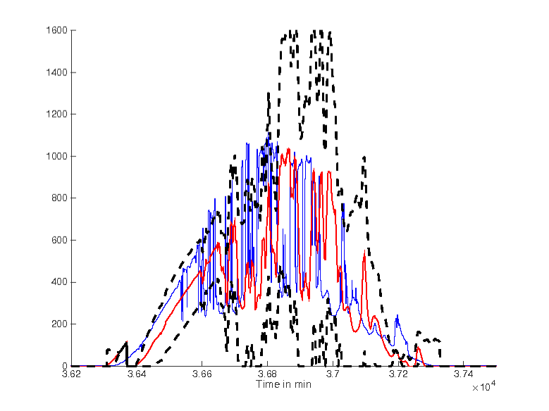
where the parameter $\alpha$ is determined here by asking that during the three last days $68\%$ of the measured data were in $\text{\bf CB}_{2,\ \text{pred$60$}}(t)$. See Figures 5 and 9 .

(a) Monthly view

(b) Zoom of 2-(a)

(c) Zoom of 2-(a)

Figure 2: February : irradiance (blue) and its prediction (red)

(a) Monthly view

(b) Zoom of 3-(a)

(c) Zoom of 3-(a)

Figure 3: February : volatilty (blue) and its trend prediction (red)

(a) Monthly view

(b) Zoom of 4-(a)

(c) Zoom of 4-(a)

Figure 4: February: irradiance (blue), its prediction (red), confidence band (black - -) (case: CB1)

(a) Monthly view

(b) Zoom of 5-(a)

(c) Zoom of 5-(a)

Figure 5: February: irradiance (blue), its prediction (red), confidence band (black - -) (case: CB2)

(a) Monthly view

(b) Zoom of 6-(a)

(c) Zoom of 6-(a)

Figure 6: June : irradiance (blue) and its prediction (red)

(a) Monthly view

(b) Zoom of 7-(a)

(c) Zoom of 7-(a)

Figure 7: June : volatilty (blue) and its trend prediction (red)

(a) Monthly view

(b) Zoom of 8-(a)

(c) Zoom of 8-(a)

Figure 8: June: irradiance (blue), its prediction (red), confidence band (black - -) (case: CB1)

(a) Monthly view

(b) Zoom of 9-(a)

(c) Zoom of 9-(a)

Figure 9: June: irradiance (blue), its prediction (red), confidence band (black - -) (case: CB2)

3 Conclusion

Improving short-term forecasting and the corresponding confidence bands will be tackled in future publications. Seasonalities (see, e.g., Fliess & Join (2015b)) will of course play some rôle.

This communication shows that a “good” forecast (see, e.g., Murphy (1993)) should incorporate a measure of risk. Since, according to Section 2.3, classic statistical confidence intervals are meaningless, we have introduced confidence bands, which do not necessitate any a priori probabilistic knowledge. Those bands will of course be further developed and applied to other domains.

The fact that no probabilistic description is needed has been already addressed in Fliess (2006); Fliess & Join (2009); Fliess, Join & Hatt (2011b). It is quite new in applied academic sciences, where a probabilistic description plays too often a key rôle. This fundamental epistemological issue ought to be further developed (see also Ayache (2010)).

The installation of the meteorological station was made possible by the project E2D2, or Énergie, Environnement & Développement Durable, which is supported by the Université de Lorraine and the Région Lorraine.

References

-
Abouaïssa, Fliess & Join (2016)
H. Abouaïssa, M. Fliess, C. Join.
On short-term traffic flow forecasting and its reliability. 8th IFAC Conf. Manufact. Model. Manag. Contr., Troyes, 2016.
Online:
https://hal.archives-ouvertes.fr/hal-01275311/en/ - Ayache (2010) E. Ayache. The Blank Swan – The End of Probability. Wiley, 2010.
- Bacher, Madsen & Nielsen (2009) P. Bacher, H. Madsen, H.A. Nielsen. Online short-term solar power forecasting. Solar Ener., 83: 1772-1783, 2009.
- Bollinger (2001) J. Bollinger. Bollinger on Bollinger Bands. McGraw-Hill, 2001.
- Bourbonnais & Terraza (2010) R. Bourbonnais, M. Terraza. Analyse des séries temporelles (3e éd.). Dunod, 2010.
- Cartier & Perrin (1995) P. Cartier, Y. Perrin. Integration over finite sets. F. & M. Diener editors: Nonstandard Analysis in Practice, pp. 195-204, Springer, 1995.
- Cryer & Chan (2008) J.D. Cryer, K.-S. Chan. Time Series Analysis: With Applications in R (2nd ed.). Springer, 2008.
- Diagne, David, Lauret, Boland & Schmutz (2013) M. Diagne, M. David, P. Lauret, J. Boland, N. Schmutz. Review of solar irradiance forecasting methods and a proposition for small-scale insular grids. Renew. Sustain. Energy Rev., 27: 65-76, 2013.
- Duchon & Hale (2012) C. Duchon, R. Hale. Time Series Analysis in Meteorology and Climatology: An Introduction. Wiley-Blackwell, 2012.
- Fliess (2006) M. Fliess. Analyse non standard du bruit. C.R. Acad. Sci. Paris Ser. I, 342: 797-802, 2006
- Fliess & Join (2009) M. Fliess, C. Join. A mathematical proof of the existence of trends in financial time series. In A. El Jai, L. Afifi, E. Zerrik, editors, Systems Theory: Modeling, Analysis and Control, pp. 43-62, Presses Universitaires de Perpignan, 2009. Online: https://hal.archives-ouvertes.fr/inria-00352834/en/
- Fliess & Join (2013) M. Fliess, C. Join. Model-free control. Int. J. Control, 86: 2228-2252, 2013.
- Fliess & Join (2015a) M. Fliess, C. Join, Towards a new viewpoint on causality for time series. ESAIM ProcS, 49: 37-52, 2015a. Online: https://hal.archives-ouvertes.fr/hal-00991942/en/
Fliess & Join (2015b)
M. Fliess, C. Join, Seasonalities and cycles in time series: A fresh look with computer experiments. Paris Finan. Manag. Conf., Paris, 2015b. Online:
https://hal.archives-ouvertes.fr/hal-01208171/en/ - Fliess, Join & Hatt (2011a) M. Fliess, C. Join, F. Hatt. Volatility made observable at last. 3es J. Identif. Modél. Expérim., Douai, 2011a. Online: https//hal.archives-ouvertes.fr/hal-00562488/en/
- Fliess, Join & Hatt (2011b) M. Fliess, C. Join, F. Hatt. A-t-on vraiment besoin d’un modèle probabiliste en ingénierie financière? Conf. Médit. Ingén. Sûre Syst. Compl., Agadir, 2011b. Online: https//hal.archives-ouvertes.fr/hal-00585152/en/
- Jama, Noura, Wahyudie & Assi (2015) M.A. Jama, H. Noura, A. Wahyudie, A. Assi. Enhancing the performance of heaving wave energy converters using model-free control approach. Renew. Energy, 83: 931-941, 2015.
- Jarque & Bera (1987) C.M. Jarque, A.K. Bera. A test for normality of observations and regression residuals. Int. Stat. Rev, 55: 163-172, 1987.
- Join, Robert & Fliess (2010) C. Join, G. Robert, M. Fliess. Vers une commande sans modèle pour aménagements hydroélectriques en cascade. 6e Conf. Internat. Francoph. Automat., Nancy, 2010. Online: http://hal.archives-ouvertes.fr/inria-00460912/en/
Join, Voyant, Fliess, Nivet, Muselli, Paoli & Chaxel (2014)
C. Join, C. Voyant, M. Fliess, M. Muselli, M.-L. Nivet, C. Paoli, F. Chaxel. Short-term solar irradiance and irradiation forecasts via different time series techniques: A preliminary study.
3rd Int. Symp. Environ. Friendly Energy Appl., Paris, 2014. Online:
https://hal.archives-ouvertes.fr/hal-01068569/en/ - Judge, Griffiths, Hill, Lütkepol & Lee (1988) G.G. Judge, W.E. Griffiths, R.C. Hill, H. Lütkepohl, T.-C. Lee. Introduction to the Theory and Practice of Econometrics (2nd ed.). Wiley, 1988.
- Kleissl (2013) J. Kleissl (Ed.). Solar Energy Forecasting and Resource Assessment. Academic Press, 2013.
- Lauret, Voyant, Soubdhari, David & Poggi (2015) P. Lauret, C. Voyant, T. Soubdhan, M. David, P. Poggi. A benchmarking of machine learning techniques for solar radiation forecasting in an insular context. Solar Energ., 112: 446-457, 2015.
- Martín, Zarzalejo, Polo, Navarro, Marchante & Cony (2010) L. Martín, L.F. Zarzalejo, J. Polo, A. Navarro, R. Marchante, M. Cony. Prediction of global solar irradiance based on time series analysis: Application to solar thermal power plants energy production planning. Solar Ener., 84: 1772-1781, 2010.
- Meuriot (2012) V. Meuriot. Une histoire des concepts des séries temporelles. Harmattan–Academia, 2012.
- Murphy (1993) A.H. Murphy, What is a good forecast? An essay on the nature of goodness in weather forecasting. Weather Forecast., 8: 281-293, 1993.
- Reikard (2009) G. Reikard. Predicting solar radiation at high resolutions: A comparison of time series forecasts. Solar Ener., 83: 342-349, 2009.
- Thode (2002) H.C. Thode, Jr. Testing for Normality. Marcel Dekker, 2002.
Trapero (2015)
J.R. Trapero. Estimation of solar irradiation prediction intervals combining volatility and kernel density estimates. ResearchGate, 2015. Online:
https://www.researchgate.net/publication/280735790 - Trapero, Kourentzes & Martin (2015) J.R. Trapero, N. Kourentzes, A. Martin. Short-term solar irradiation forecasting based on dynamic harmonic regression. Energy, 84: 289-295, 2015.
Voyant, Join, Fliess, Nivet, Muselli & Paoli (2015)
C. Voyant, C. Join, M. Fliess, M.-L. Nivet, M. Muselli, & C. Paoli. On meteorological forecasts for energy management and large historical data: A first look.
Renew. Ener. Power Quality J., 13, 2015. Online:
https//hal.archives-ouvertes.fr/hal-01093635/en/ - Voyant, Muselli & Nivet (2011) C. Voyant, M. Muselli, C. Paoli, M.-L. Nivet. Optimization of an artificial neural network dedicated to the multivariate forecasting of daily global radiation. Energy, vol. 36: 348-359, 2011.
- Voyant, Paoli, Muselli & Nivet (2013) C. Voyant, C. Paoli, M. Muselli, M.-L. Nivet. Multi-horizon solar radiation forecasting for Mediterranean locations using time series models. Renew. Sustain. Energy Rev., 28: 44-52, 2013.
- Voyant, Soubdhan, Lauret, David & Muselli (2015) C. Voyant, T. Soubdhan, P. Lauret, M. David, M. Muselli. Statistical parameters as a means to a priori assess the accuracy of solar forecasting models. Energy, 90: 671-679, 2015.
- Willink (2013) R. Willink. Measurement Uncertainty and Probability. Cambridge University Press, 2013.
- Yang, Sharma, Ye, Lim, Zhao & Aryaputer (2015) D. Yang, V. Sharma, Z. Ye, L.I. Lim, L. Zhao, A.W. Aryaputer. Forecasting of global horizontal irradiance by exponential smoothing, using decompositions. Energy, 81: 111-119, 2015.