Contextual LSTM (CLSTM) models for
Large scale NLP tasks

Abstract

Documents exhibit sequential structure at multiple levels of abstraction (e.g., sentences, paragraphs, sections). These abstractions constitute a natural hierarchy for representing the context in which to infer the meaning of words and larger fragments of text. In this paper, we present CLSTM (Contextual LSTM), an extension of the recurrent neural network LSTM (Long-Short Term Memory) model, where we incorporate contextual features (e.g., topics) into the model. We evaluate CLSTM on three specific NLP tasks: word prediction, next sentence selection, and sentence topic prediction. Results from experiments run on two corpora, English documents in Wikipedia and a subset of articles from a recent snapshot of English Google News, indicate that using both words and topics as features improves performance of the CLSTM models over baseline LSTM models for these tasks. For example on the next sentence selection task, we get relative accuracy improvements of 21% for the Wikipedia dataset and 18% for the Google News dataset. This clearly demonstrates the significant benefit of using context appropriately in natural language (NL) tasks. This has implications for a wide variety of NL applications like question answering, sentence completion, paraphrase generation, and next utterance prediction in dialog systems.

1 Introduction

Documents have sequential structure at different hierarchical levels of abstraction: a document is typically composed of a sequence of sections that have a sequence of paragraphs, a paragraph is essentially a sequence of sentences, each sentence has sequences of phrases that are comprised of a sequence of words, etc. Capturing this hierarchical sequential structure in a language model (LM) [30] can potentially give the model more predictive accuracy, as we have seen in previous work [12, 13, 25, 33, 48].

A useful aspect of text that can be utilized to improve the performance of LMs is long-range context. For example, let us consider the following three text segments:

1) Sir Ahmed Salman Rushdie is a British Indian novelist and essayist. He is said to combine magical realism with historical fiction.

2) Calvin Harris & HAIM combine their powers for a magical music video.

3) Herbs have enormous magical power, as they hold the earth’s energy within them.

Consider an LM that is trained on a dataset having the example sentences given above — given the word “magical”, what should be the most likely next word according to the LM: realism, music, or power? In this example, that would depend on the longer-range context of the segment in which the word “magical” occurs. One way in which the context can be captured succinctly is by using the topic of the text segment (e.g., topic of the sentence, paragraph). If the context has the topic “literature”, the most likely next word should be “realism”. This observation motivated us to explore the use of topics of text segments to capture hierarchical and long-range context of text in LMs.

In this paper, we consider Long-Short Term Memory (LSTM) models [20], a specific kind of Recurrent Neural Networks (RNNs). The LSTM model and its different variants have achieved impressive performance in different sequence learning problems in speech, image, music and text analysis [15, 16, 19, 36, 39, 40, 42, 43, 45], where it is useful in capturing long-range dependencies in sequences. LSTMs substantially improve our ability to handle long-range dependencies, though they still have some limitations in this regard [6, 12].

RNN-based language models (RNN-LMs) were proposed by Mikolov et al. [32], and in particular the variant using LSTMs was introduced by Sundermeyer et al. [38]. In this paper, we work with LSTM-based LMs. Typically LSTMs used for language modeling consider only words as features. Mikolov et al. [31] proposed a conditional RNN-LM for adding context — we extend this approach of using context in RNN-LMs to LSTMs, train the LSTM models on large-scale data, and propose new tasks beyond next work prediction.

We incorporate contextual features (namely, topics based on different segments of text) into the LSTM model, and call the resulting model Contextual LSTM (CLSTM). In this work we evaluate how adding contextual features in the CLSTM improves the following tasks:

1) Word prediction: Given the words and topic seen so far in the current sentence, predict the most likely next word. This task is important for sentence completion in applications like predictive keyboard, where long-range context can improve word/phrase prediction during text entry on a mobile phone.

2) Next sentence selection: Given a sequence of sentences, find the most likely next sentence from a set of candidates. This is an important task in question/answering, where topic can be useful in selecting the best answer from a set of template answers. This task is also relevant in other applications like Smart Reply [7], for predicting the best response to an email from a set of candidate responses.

3) Sentence topic prediction: Given the words and topic of the current sentence, predict the topic of the next sentence. We consider two scenarios: (a) where we don’t know the words of the next sentence, (b) where we know the words of the next sentence. Scenario (a) is relevant for applications where we don’t know the words of a user’s next utterance, e.g., while predicting the topic of response of the user of a dialog system, which is useful in knowing the intent of the user; in scenario (b) we try to predict the topic/intent of an utterance, which is common in a topic modeling task.

The main contributions of this paper are as follows:

1) We propose a new Contextual LSTM (CLSTM) model, and demonstrate how it can be useful in tasks like word prediction, next sentence scoring and sentence topic prediction – our experiments show that incorporating context into an LSTM model (via the CLSTM) gives improvements compared to a baseline LSTM model. This can have potential impact for a wide variety of NLP applications where these tasks are relevant, e.g. sentence completion, question/answering, paraphrase generation, dialog systems.

2) We trained the CLSTM (and the corresponding baseline LSTM) models on two large-scale document corpora: English documents in Wikipedia, and a recent snapshot of English Google News documents. The vocabulary we handled in the modeling here was also large: 130K words for Wikipedia, 100K for Google news. Our experiments and analysis demonstrate that the CLSTM model that combines the power of topics with word-level features yields significant performance gains over a strong baseline LSTM model that uses only word-level features. For example, in the next sentence selection task, CLSTM gets a performance improvement of 21% and 18% respectively over the LSTM model on the English Wikipedia and Google News datasets.

3) We show initial promising results with a model where we learn the thought embedding in an unsupervised manner through the model structure, instead of using supervised extraneous topic as side information (details in Section 5.4).

2 Related Work

There are various approaches that try to fit a generative model for full documents. These include models that capture the content structure using Hidden Markov Models (HMMs) [3], or semantic parsing techniques to identify the underlying meanings in text segments [29]. Hierarchical models have been used successfully in many applications, including hierarchical Bayesian models [10, 27], hierarchical probabilistic models [37], hierarchical HMMs [14] and hierarchical CRFs [35].

As mentioned in Section 1, RNN-based language models (RNN-LMs) were proposed by Mikolov et al. [32], and the variant using LSTMs was introduced by Sundermeyer et al. [38] – in this paper, we work with LSTM-based LMs. Mikolov et al. [31] proposed a conditional RNN-LM for adding context — we extend this approach of using context in RNN-LMs to LSTMs.

Recent advances in deep learning can model hierarchical structure using deep belief networks [21, 48, 49, 46], especially using a hierarchical recurrent neural network (RNN) framework. In Clockwork RNNs [24] the hidden layer is partitioned into separate modules, each processing inputs at its own individual temporal granularity. Connectionist Temporal Classification or CTC [18] does not explicitly segment the input in the hidden layer – it instead uses a forward-backward algorithm to sum over all possible segments, and determines the normalized probability of the target sequence given the input sequence. Other approaches include a hybrid NN-HMM model [1], where the temporal dependency is handled by an HMM and the dependency between adjacent frames is handled by a neural net (NN). In this model, each node of the convolutional hidden layer corresponds to a higher-level feature.

Some NN models have also used context for modeling text. Paragraph vectors [8, 26] propose an unsupervised algorithm that learns a latent variable from a sample of words from the context of a word, and uses the learned latent context representation as an auxiliary input to an underlying skip-gram or Continuous Bag-of-words (CBOW) model. Another model that uses the context of a word infers the Latent Dirichlet Allocation (LDA) topics of the context before a word and uses those to modify a RNN model predicting the word [31].

Tree-structured LSTMs [41, 48] extend chain-structured LSTMs to the tree structure and propose a principled approach of considering long-distance interaction over hierarchies, e.g., language or image parse structures. Convolution networks have been used for multi-level text understanding, starting from character-level inputs all the way to abstract text concepts [47]. Skip thought vectors have also been used to train an encoder-decoder model that tries to reconstruct the surrounding sentences of an encoded passage [23].

Other related work include Document Context Language models [22], where the authors have multi-level recurrent neural network language models that incorporate context from within a sentence and from previous sentences. Lin et al. [28] use a hierarchical RNN structure for document-level as well as sentence-level modeling – they evaluate their models using word prediction perplexity, as well as an approach of coherence evaluation by trying to predict sentence-level ordering in a document.

In this work, we explore the use of long-range hierarchical signals (e.g., sentence level or paragraph level topic) for text analysis using a LSTM-based sequence model, on large-scale data — to the best of our knowledge this kind of contextual LSTM models, which model the context using a 2-level LSTM architecture, have not been trained before at scale on text data for the NLP tasks mentioned in Section 1.

3 Word Prediction

Of the three different tasks outlined in Section 1, we focus first on the word prediction task, where the goal is to predict the next word in a sentence given the words and context (captured via topic) seen previously.

Let $s_{i}$ be the $i^{th}$ sentence in a sequence of sentences, $w_{i,j}$ be the $j^{th}$ word of sentence $s_{i}$, $n_{i}$ be the number of words in $s_{i}$, and $w_{i,j}\ldots w_{i,k}$ indicate the sequence of words from word $j$ to word $k$ in sentence $i$. Note that sentence $s_{i}$ is equivalent to the sequence of words $w_{i,0}\ldots w_{i,n_{i}-1}$. Let $T$ be the random variable denoting the topic – it is computed based on a particular subsequence of words seen from the first word of the sequence ($w_{0,0}$) to the current word ($w_{i,j}$). This topic can be based on the current sentence segment (i.e., $T=Topic(w_{i,0}\ldots w_{i,j-1})$), or the previous sentence (i.e., $T=Topic(w_{i-1,0}\ldots w_{i-1,n_{i-1}})$), etc. Details regarding the topic computation are outlined in Section 3.2.

Using this notation, the word prediction task in our case can be specified as follows: given a model with parameters $\Theta$, words $w_{0,0}\ldots w_{i,j}$ and the topic $T$ computed from a subsequence of the words from the beginning of the sequence, find the next word $w_{i,j+1}$ that maximizes the probability: $P(w_{i,j+1}|w_{0,0}\ldots w_{i,j},T,\Theta)$.

3.1 Model

For our approach, as explained before, we introduce the power of context into a standard LSTM model. LSTM is a recurrent neural network that is useful for capturing long-range dependencies in sequences. The LSTM model has multiple LSTM cells, where each LSTM cell models the digital memory in a neural network. It has gates that allow the LSTM to store and access information over time. For example, the input/output gates control cell input/output, while the forget gate controls the state of the cell.

The word-prediction LSTM model was implemented in the large-scale distributed Google Brain framework [9]. The model takes words encoded in 1-hot encoding from the input, converts them to an embedding vector, and consumes the word vectors one at a time. The model is trained to predict the next word, given a sequence of words already seen. The core algorithm used to train the LSTM parameters is BPTT [44], using a softmax layer that uses the id of the next word as the ground truth.

To adapt the LSTM cell that takes words to a CLSTM cell that takes as input both words and topics, we modify the equations representing the operations of the LSTM cell [17] to add the topic vector $T$ to the input gate, forget gate, cell and output gate ($T$ is the embedding of the discrete topic vector). In each of the following equations, the term in bold is the modification made to the original LSTM equation.

$$i_{t} = \sigma(W_{xi}x_{t}+W_{hi}h_{t-1}+W_{ci}c_{t-1}+b_{i}+\bf{W_{Ti}T)}$$

$$f_{t} = \sigma(W_{xf}x_{t}+W_{hf}h_{t-1}+W_{cf}c_{t-1}+b_{f}+\bf{W_{Ti}T)}$$

$$c_{t} = f_{t}c_{t-1}+i_{t}\tanh(W_{xc}x_{t}+W_{hc}h_{t-1}+b_{c}+\bf{W_{Ti}T)}$$

$$o_{t} = \sigma(W_{xo}x_{t}+W_{ho}h_{t-1}+W_{co}c_{t}+b_{o}+\bf{W_{Ti}T)}$$

$$h_{t} = o_{t}\tanh(c_{t})$$ (1)

In these equations $i$, $f$ and $o$ are the input gate, forget gate and output gate respectively, $x$ is the input, $b$ is the bias term, $c$ is the cell memory, and $h$ is the output. As an example, consider the input gate equation:

$$i_{t}= \sigma(W_{xi}x_{t}+W_{hi}h_{t-1}+W_{ci}c_{t-1}+b_{i})$$

$$= \sigma([W_{xi}\ W_{hi}\ W_{ci}\ 1][x_{t}\ h_{t-1}\ c_{t-1}\ b_{i}]^{T})$$ (2)

When we add the topic signal $T$ to the input gate, the equation is modified to:

$$i_{t}= \sigma(W_{xi}x_{t}+W_{hi}h_{t-1}+W_{ci}c_{t-1}+b_{i}+W_{Ti}T)$$

$$= \sigma([W_{xi}\ W_{Ti}\ W_{hi}\ W_{ci}\ 1][x_{t}\ T\ h_{t-1}\ c_{t-1}\ b_{i}]^{T})$$ (3)

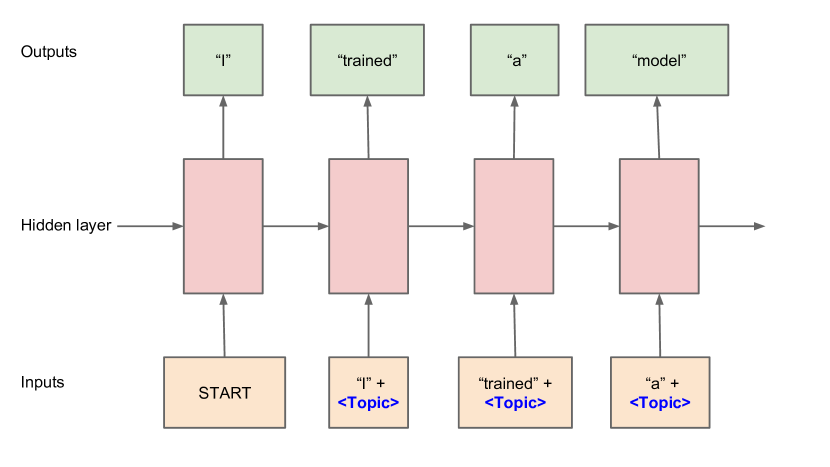
Comparing the last two equations, Equations 2 and 3, we see that having a topic vector $T$ added into the CLSTM cell is equivalent to considering a composite input $[x_{i}$  $T]$ to the LSTM cell that concatenates the word embedding and topic embedding vectors. This approach of concatenating topic and word embeddings in the input worked better in practice than other strategies for combining topics with words. Figure 1 shows the schematic figure of a CLSTM model that considers both word and topic input vectors.

Note that we add the topic input to each LSTM cell since each LSTM cell can potentially have a different topic. For example, when the topic is based on the sentence segment seen so far (see Section 3.3.1), the topic is based on the current sentence prefix — so, each LSTM cell can potentially have a different topic. Note that in some setups each LSTM cell in a layer could have the same topic, e.g., when the topic is derived from the words in the previous sentence.

Figure 1: CLSTM model ($<$Topic$>$ = topic input)

3.2 HTM: Supervised Topic Labels

The topics of the text segments can be estimated using different unsupervised methods (e.g., clustering) or supervised methods (e.g., hierarchical classification). For the word prediction task we use HTM, a hierarchical topic model for supervised classification of text into a hierarchy of topic categories, based on the Google Rephil large-scale clustering tool [34]. There are about 750 categories at the leaf level of the HTM topic hierarchy. Given a segment of text, HTM gives a probability distribution over the categories in the hierarchy, including both leaf and intermediate categories. We currently choose highest probability topic as the most-likely category of the text segment.

3.3 Experiments

Figure 2: Hierarchical Features used in CLSTM models

3.3.1 Features

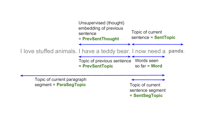
We trained different types of CLSTM models for the word prediction task. The different types of features used in the different CLSTM models are shown schematically in Figure 2. The hierarchical features that we used in different variants of the word prediction model are:

1. PrevSentTopic = TopicID of the topic computed based on all the words of the previous sentence, i.e., $T=Topic(w_{i-1,0}\ldots w_{i-1,n_{i-1}-1})$.

2. SentSegTopic = TopicID of the topic computed based on the words of the current sentence prefix until the current word, i.e., $T=Topic(w_{i,0}\ldots w_{i,j})$.

3. ParaSegTopic = TopicID of the topic computed based on the paragraph prefix until the current word, i.e., $T=Topic(w_{0,0}\ldots w_{i,j})$.

where $T$ is defined in Section 3.

3.3.2 Datasets

For our experiments, we used the whole English corpus from Wikipedia (snapshot from 2014/09/17). There were 4.7 million documents in the Wikipedia dataset, which we randomly divided into 3 parts: 80% was used as train, 10% as validation and 10% as test set. Some relevant statistics of the train, test and validation data sets of the Wikipedia corpus are given in Table 1.

Table 1: Wikipedia Data Statistics (M=million)

Dataset	#Para	#Sent	#Word
Train (80%)	23M	72M	1400M
Validation (10%)	2.9M	8.9M	177M
Test (10%)	3M	9M	178M

We created the vocabulary from the words in the training data, filtering out words that occurred less than a particular threshold count in the total dataset (threshold was 200 for Wikipedia). This resulted in a vocabulary with 129K unique terms, giving us an out-of-vocabulary rate of 3% on the validation dataset.

For different types of text segments (e.g., segment, sentence, paragraph) in the training data, we queried HTM and got the most likely topic category. That gave us a total of $\approx$1600 topic categories in the dataset.

3.3.3 Results

Table 2: Test Set Perplexity for Word Prediction task

Input	Num Hidden	Num Hidden	Num Hidden
Features	Units = 256	Units = 512	Units = 1024
Word	38.56	32.04	27.66
Word + PrevSentTopic	37.79	31.44	27.81
Word + SentSegTopic	38.04	31.28	27.34
Word + ParaSegTopic	38.02	31.41	27.30
Word + PrevSentTopic + SentSegTopic	38.11	31.22	27.31
Word + SentSegTopic + ParaSegTopic	37.65	31.02	27.10

We trained different CLSTM models with different feature variants till convergence, and evaluated their perplexity on the holdout test data. Here are some key observations about the results (details in Table 2):

1) The “Word + SentSegTopic + ParaSegTopic” CLSTM model is the best model, getting the best perplexity. This particular LSTM model uses both sentence-level and paragraph-level topics as features, implying that both local and long-range context is important for getting the best performance.

2) When current segment topic is present, the topic of the previous sentence does not matter.

3) As we increased the number of hidden units, the performance started improving. However, beyond 1024 hidden units, there were diminishing returns — the gain in performance was out-weighed by the substantial increase in computational overhead.

Note that we also trained a distributed n-gram model with “stupid backoff” smoothing [4] on the Wikipedia dataset, and it gave a perplexity of $\approx$80 on the validation set. We did not train a n-gram model with Knesner-Ney (KN) smoothing on the Wikipedia data, but on the Google News data (from a particular snapshot) the KN smoothed n-gram model gave a perplexity of 74 (using 5-grams).

Note that we were not able to compare our CLSTM models to other existing techniques for integrating topic information into LSTM models (e.g., Mikolov et al. [31]), since we didn’t have access to implementations of these approaches that can scale to the vocabulary sizes ($\approx$ 100K) and dataset sizes we worked with (e.g., English Wikipedia, Google News snapshot). Hence, we used a finely-tuned LSTM model as a baseline, which we also trained at scale on these datasets.

4 Next Sentence Selection

Figure 3: Next Sentence Selection Example

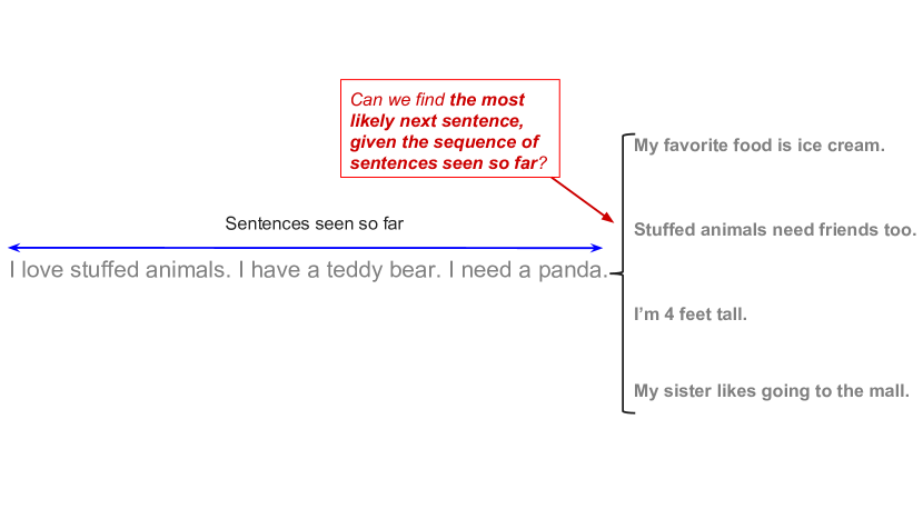
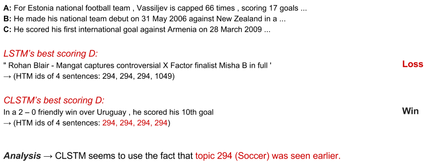
We next focus on the next sentence scoring task, where we are given a sequence of sentences and the goal is to find the most probable next sentence from a set of candidate sentences. An example of this task is shown in Figure 3. The task can be stated as follows: given a model with parameters $\Theta$, a sequence of $p-1$ sentences $s_{0}\ldots s_{p-2}$ (with their corresponding topics $T_{0}\ldots T_{p-2}$), find the most likely next sentence $s_{p-1}$ from a candidate set of next sentences $S$, such that:

$$s_{p-1}=\arg\max_{s\in S}P(s|s_{0}\ldots s_{p-2},T_{0}\ldots T_{p-2},\Theta).$$

4.1 Problem Instantiation

Suppose we are given a set of sequences, where each sequence consists of 4 sentences (i.e., we consider $p$=4). Let each sequence be $S_{i}=<A_{i}B_{i}C_{i}D_{i}>$, and the set of sequences be $\{S_{1},\ldots,S_{k}\}$. Given the prefix $A_{i}B_{i}C_{i}$ of the sequence $S_{i}$ as context (which we will denote to be $Context_{i}$), we consider the task of correctly identifying the next sentence $D_{i}$ from a candidate set of sentences: $\{D_{0},D_{1},\ldots,D_{k-1}\}$. For each sequence $S_{i}$, we compute the accuracy of identifying the next sentence correctly. The accuracy of the model in detecting the correct next sentence is computed over the set of sequences $\{S_{1},\ldots,S_{k}\}$.

4.2 Approach

We train LSTM and CLSTM models specifically for the next sentence prediction task. Given the context $Context_{i}$, the models find the $D_{i}$ among the set $\{D_{0}\ldots D_{k-1}\}$ that gives the maximum (normalized) score, defined as follows:

$$\forall i,score=\frac{P(D_{i}|Context_{i})}{\frac{1}{k}\sum_{j=0}^{k-1}P(D_{i}|Context_{j})}$$ (4)

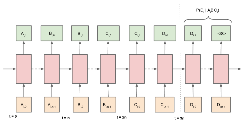
In the above score, the conditional probability terms are estimated using inference on the LSTM and CLSTM models. In the numerator, the probability of the word sequence in $D_{i}$, given the prefix context $Context_{i}$, is estimated by running inference on a model whose state is already seeded by the sequence $A_{i}B_{i}C_{i}$ (as shown in Figure 4). The normalizer term $\frac{1}{k}\sum_{j=0}^{k-1}P(D_{i}|Context_{j})$ in the denominator of Equation 4 is the point estimate of the marginal probability $P(D_{i})$ computed over the set of sequences, where the prior probability of each prefix context is assumed equal, i.e., $P(Context_{j})=\frac{1}{k},j\in[0,k-1]$. The normalizer term adjusts the score to account for the popularity of a sentence $D_{i}$ that naturally has a high marginal probability $P(D_{i})$ — we do not allow the popularity of $D_{i}$ to lead to a high score.

Figure 4: Next Sentence Scoring in CLSTM model

Note that for task of next sentence scoring, it’s ok to use words of the next sentence when selecting the “best” next sentence. This is because in the task, the possible alternatives are all provided to the model, and the main goal of the model is scoring the alternatives and selecting the best one. This setting is seen in some real-world applications, e.g., predicting the best response to an email from a set of candidate responses [7].

4.3 Model

We trained a baseline LSTM model on the words of $A_{i}$, $B_{i}$ and $C_{i}$ to predict the words of $D_{i}$. The CLSTM model uses words from $A_{i}$, $B_{i}$, $C_{i}$, and topics of $A_{i}$, $B_{i}$, $C_{i}$ and $D_{i}$, to predict the words of $D_{i}$. Note that in this case we can use the topic of $D_{i}$ since all the candidate next sentences are given as input in the next sentence scoring task.

For 1024 hidden units, the perplexity of the baseline LSTM model after convergence of model training is 27.66, while the perplexity of the CLSTM model at convergence is 24.81. This relative win of 10.3% in an intrinsic evaluation measure (like perplexity) was the basis for confidence in expecting good performance when using this CLSTM model for the next sentence scoring task.

4.4 Experimental Results

We ran next sentence scoring experiments with a dataset generated from the test set of the corpora. We divide the test dataset into 100 non-overlapping subsets. To create the dataset for next sentence scoring, we did the following: (a) sample 50 sentence sequences $<A_{i}B_{i}C_{i}D_{i}>$ from 50 separate paragraphs, randomly sampled from 1 subset of the test set – we call this a block; (b) consider 100 such blocks in the next sentence scoring dataset. So, overall there are 5000 sentence sequences in the final dataset. For each sequence prefix $A_{i}B_{i}C_{i}$, the model has to choose the best next sentence $D_{i}$ from the competing set of next sentences.

Table 3: Accuracy of CLSTM on next sentence scoring

LSTM	CLSTM	Accuracy Increase
$52\%\pm 2\%$	$63\%\pm 2\%$	$21\%\pm 9\%$

The average accuracy of the baseline LSTM model on this dataset is $52\%$, while the average accuracy of the CLSTM model using word + sentence-level topic features is $63\%$ (as shown in Table 3). So the CLSTM model has an average improvement of $21\%$ over the LSTM model on this dataset. Note that on this task, the average accuracy of a random predictor that randomly picks the next sentence from a set of candidate sentences would be $2\%$.

We also ran other experiments, where the negatives (i.e., 49 other sentences in the set of 50) were not chosen randomly — in one case we considered all the 50 sentences to come from the same HTM topic, making the task of selecting the best sentence more difficult. In this case, as expected, the gain from using the context in CLSTM was larger — the CLSTM model gave larger improvement over the baseline LSTM model than in the case of having a random set of negatives.

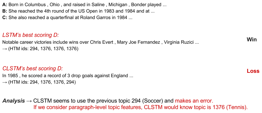
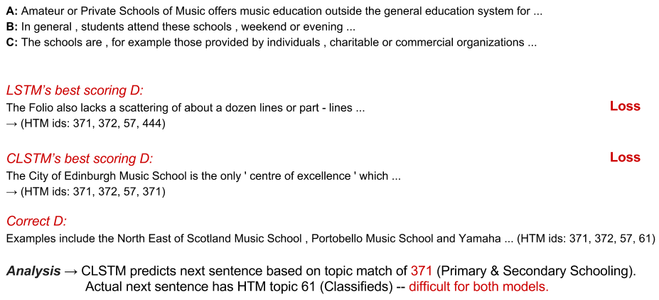
4.5 Error Analysis

Figures 5-7 analyze different types of errors made by the LSTM and the CLSTM models, using samples drawn from the test dataset.

Figure 5: Error Type A: CLSTM correct, LSTM incorrect

Figure 6: Error Type B: CLSTM incorrect, LSTM correct

Figure 7: Error Type C: CLSTM and LSTM both incorrect

5 Sentence Topic Prediction

The final task we consider is the following: if we are given the words and the topic of the current sentence, can we predict the topic of the next sentence? This is an interesting problem for dialog systems, where we ask the question: given the utterance of a speaker, can we predict the topic of their next utterance? This can be used in various applications in dialog systems, e.g., intent modeling.

The sentence topic prediction problem can be formulated as follows: given a model with parameters $\Theta$, words in the sentence $s_{i}$ and corresponding topic $T_{i}$, find the next sentence topic $T_{i+1}$ that maximizes the following probability – $P(T_{i+1}|s_{i},T_{i},\Theta)$. Note that in this case we train a model to predict the topic target instead of the joint word/topic target, since we empirically determined that training a model with a joint target gave lower accuracy in predicting the topic compared to a model that only tries to predict the topic as a target.

5.1 Model

For the sentence topic prediction task, we determined through ablation experiments that the unrolled model architecture, where each sentence in a paragraph is modeled by a separate LSTM model, has better performance than the rolled-up model architecture used for word prediction where the sentences in a paragraph are input to a single LSTM.

5.2 Experiments

In our experiments we used the output of HTM as the topic of each sentence. Ideally we would associate a “supervised topic” with each sentence (e.g., the supervision provided by human raters). However, due to the difficulty of getting such human ratings at scale, we used the HTM model to find topics for the sentences. Note that the HTM model is trained on human ratings.

We trained 2 baseline models on this dataset. The Word model uses the words of the current sentence to predict the topic of the next sentence – it determines how well we can predict the topic of the next sentence, given the words of the current sentence. We also trained another baseline model, SentTopic, which uses the sentence topic of the current sentence to predict the topic of the next sentence – the performance of this model will give us an idea of the inherent difficulty of the task of topic prediction. We trained a CLSTM model (Word+SentTopic) that uses both words and topic of the current sentence to predict the topic of the next sentence. Figure 2 shows the hierarchical features used in the CLSTM model. We trained all models with different number of hidden units: 256, 512, 1024. Each model was trained till convergence. Table 4 shows the comparison of the perplexity of the different models. The CLSTM model beats the baseline SentTopic model by more than 12%, showing that using hierarchical features is useful for the task of sentence topic prediction too.

Table 4: Test Set Perplexity for sentence topic prediction (W=Word, ST=SentTopic)

Inputs	#Hidden	#Hidden	#Hidden
	units=256	units=512	units=1024
W	24.50	23.63	23.29
ST	2.75	2.75	2.76
W + ST	2.43	2.41	2.43

5.3 Comparison to BOW-DNN baseline

For the task of sentence topic prediction, we also compared the CLSTM model to a Bag-of-Words Deep Neural Network (BOW-DNN) baseline [2]. The BOW-DNN model extracts bag of words from the input text, and a DNN layer is used to extract higher-level features from the bag of words. For this experiment, the task setup we considered was slightly different in order to facilitate more direct comparison. The goal was to predict the topic of the next sentence, given words of the next sentence. The BOW-DNN model was trained only on word features, and got a test set perplexity of 16.5 on predicting the sentence topic. The CLSTM model, trained on word and topic-level features, got a perplexity of 15.3 on the same test set using 1024 hidden units, thus outperforming the BOW-DNN model by 7.3%.

5.4 Using Unsupervised Topic Signals

Figure 8: CLSTM model with Thought Vector

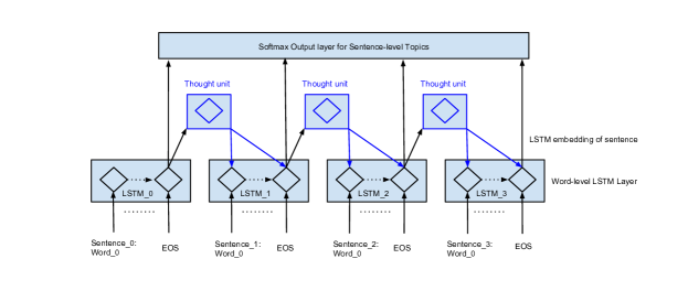
In our experiments with topic features, we have so far considered supervised topic categories obtained from an extraneous source (namely, HTM). One question arises: if we do not use extraneous topics to summarize long-range context, would we get any improvements in performance with unsupervised topic signals? To answer this question, we experimented with “thought embeddings” that are intrinsically generated from the previous context. Here, the thought embedding from the previous LSTM is used as the topic feature in the current LSTM (as shown in Figure 8), when making predictions of the topic of the next sentence – we call this context-based thought embedding the “thought vector”.

In our approach, the thought vector inferred from the LSTM encoding of sentence $n-1$ is used as a feature for the LSTM for sentence $n$, in a recurrent fashion. Note that the LSTMs for each sentence in Figure 8 are effectively connected into one long chain, since we don’t reset the hidden state at the end of each sentence — so the LSTM for the current sentence has access to the LSTM state of the previous sentence (and hence indirectly to its topic). But we found that directly adding the topic of the previous sentence to all the LSTM cells of the current sentence is beneficial, since it constraints all the current LSTM cells during training and explicitly adds a bias to the model. Our experiments showed that it’s beneficial to denoise the thought vector signal using a low-dimensional embedding, by adding roundoff-based projection. Initial experiments using thought vector for sentence-topic prediction look promising. A CLSTM model that used word along with thought vector (PrevSentThought feature in the model) from the previous sentence as features gave a 3% improvement in perplexity compared to a baseline LSTM model that used only words as features. Table 5 shows the detailed results.

When we used thought vectors, our results improved over using a word-only model but fell short of a CLSTM model that used both words and context topics derived from HTM. In the future, we would like to do more extensive experiments using better low-dimensional projections (e.g., using clustering or bottleneck mechanisms), so that we can get comparable performance to supervised topic modeling approaches like HTM.

Another point to note — we have used HTM as a topic model in our experiments as that was readily available to us. However, the CLSTM model can also use other types of context topic vectors generated by different kinds of topic modeling approaches, e.g., LDA, KMeans.

6 Results on Google News data

We also ran experiments on a sample of documents taken from a recent (2015/07/06) snapshot of the internal Google News English corpus. This subset had 4.3 million documents, which we divided into train, test and validation datasets. Some relevant statistics of the datasets are given in Table 6. We filtered out words that occurred less than 100 times, giving us a vocabulary of 100K terms.

Table 5: Test Set Perplexity for sentence topic prediction using Thought vector (W=Word, PST=PrevSentThought)

Inputs	#Hidden	#Hidden	#Hidden
	units=256	units=512	units=1024
W	24.50	23.63	23.29
W + PST	24.38	23.03	22.59

Table 6: Statistics of Google News dataset (M=million)

Dataset	#Para	#Sent	#Word
Train (80%)	6.4M	70.5M	1300M
Validation (10%)	0.8M	8.8M	169M
Test (10%)	0.8M	8.8M	170M

We trained the baseline LSTM and CLSTM models for the different tasks, each having 1024 hidden units. Here are the key results:

1) Word prediction task: LSTM using only words as features had perplexity of $\approx$ 37. CLSTM improves on LSTM by $\approx$ 2%, using words, sentence segment topics and paragraph sentence topics.

2) Next sentence selection task: LSTM gave an accuracy of $\approx$ 39%. CLSTM had an accuracy of $\approx$ 46%, giving a 18% improvement on average.

3) Next sentence topic prediction task: LSTM using only current sentence topic as feature gave perplexity of $\approx$ 5. CLSTM improves on LSTM by $\approx$ 9%, using word and current sentence topic as features.

As we see, we get similar improvements of CLSTM model over LSTM model for both the Wikipedia and Google News datasets, for each of the chosen NLP tasks.

7 Conclusions

We have shown how using contextual features in a CLSTM model can be beneficial for different NLP tasks like word prediction, next sentence selection and topic prediction. For the word prediction task CLSTM improves on state-of-the-art LSTM by 2-3% on perplexity, for the next sentence selection task CLSTM improves on LSTM by $\approx$20% on accuracy on average, while for the topic prediction task CLSTM improves on state-of-the-art LSTM by $\approx$10% (and improves on BOW-DNN by $\approx$7%). These gains are all quite significant and we get similar gains on the Google News dataset (Section 6), which shows the generalizability of our approach. Initial results using unsupervised topic signal using with vectors, instead of supervised topic models, are promising. The gains obtained by using the context in the CLSTM model has major implications of performance improvements in multiple important NLP applications, ranging from sentence completion, question/answering, and paraphrase generation to different applications in dialog systems.

8 Future Work

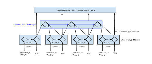
Our initial experiments on using unsupervised thought vectors for capturing long-range context in CLSTM models gave promising results. A natural extension of the thought vector model in Figure 8 is a model that has a connection between the hidden layers, to be able to model the “continuity of thought”. Figure 9 shows one such hierarchical LSTM (HLSTM) model, which has a 2-level hierarchy: a lower-level LSTM for modeling the words in a sentence, and a higher-level LSTM for modeling the sentences in a paragraph. The thought vector connection from the LSTM cell in layer $n$ to the LSTM cells in layer $n-1$ (corresponding to the next sentence) enables concepts from the previous context to be propagated forward, enabling the “thought” vector of a sentence to influence words of the next sentence. The connection between the sentence-level hidden nodes also allows the model to capture the continuity of thought. We would like to experiment with this model in the future.

Figure 9: CLSTM model with Thought Vector and Sentence-level LSTM

We would also like to explore the benefits of contextual features in other applications of language modeling, e.g., generating better paraphrases by using word and topic features. Another interesting application could be using topic-level signals in conversation modeling, e.g., using Dialog Acts as a topic-level feature for next utterance prediction.

Acknowledgments: We would like to thank Ray Kurzweil, Geoffrey Hinton, Dan Bikel, Lukasz Kaiser and Javier Snaider for useful feedback on this work. We would also like to thank Louis Shao and Yun-hsuan Sung for help in running some experiments.

References

- [1] Ossama Abdel-Hamid, Abdel rahman Mohamed, Hui Jiang, and Gerald Penn. Applying convolutional neural networks concepts to hybrid NN-HMM model for speech recognition. In ICASSP, 2012.
- [2] Yalong Bai, Wei Yu, Tianjun Xiao, Chang Xu, Kuiyuan Yang, Wei-Ying Ma, and Tiejun Zhao. Bag-of-words based deep neural network for image retrieval. In Proc. of ACM Intl. Conf. on Multimedia, 2014.
- [3] Regina Barzilay and Lillian Lee. Catching the drift: Probabilistic content models, with applications to generation and summarization. In HLT-NAACL, 2004.
- [4] Thorsten Brants, Ashok C. Popat, Peng Xu, Franz J. Och, and Jeffrey Dean. Large language models in machine translation. In EMNLP, 2007.
- [5] Ciprian Chelba, Tomas Mikolov, Mike Schuster, Qi Ge, Thorsten Brants, and Phillipp Koehn. One billion word benchmark for measuring progress in statistical language modeling. CoRR, abs/1312.3005, 2013.
- [6] K. Cho, B. Merriënboer, C. Gulcehre, F. Bougares, H. Schwenk, and Y. Bengio. Learning phrase representations using rnn encoder-decoder for statistical machine translation. CoRR, arXiv:406.1078, 2014.
- [7] Greg Corrado. Smart Reply. http://googleresearch.blogspot.com/2015/11/computer-respond-to-this-email.html, 2015.
- [8] Andrew M Dai, Christopher Olah, Quoc V Le, and Greg S Corrado. Document embedding with paragraph vectors. NIPS Deep Learning Workshop, 2014.
- [9] Jeffrey Dean, Greg S. Corrado, Rajat Monga, Kai Chen, Matthieu Devin, Quoc V. Le, Mark Z. Mao, Marc’Aurelio Ranzato, Andrew Senior, Paul Tucker, Ke Yang, , and Andrew Y. Ng. Large scale distributed deep networks. In NIPS, 2012.
- [10] Thomas Dean. Learning invariant features using inertial priors. Annals of Mathematics and Artificial Intelligence, 47(3-4):223–250, August 2006.
- [11] DL4J. Thought vectors, deep learning & the future of AI. http://deeplearning4j.org/thoughtvectors.html, 2015.
- [12] Salah El Hihi and Yoshua Bengio. Hierarchical recurrent neural networks for long-term dependencies. In NIPS, 1996.
- [13] Santiago Fernández, Alex Graves, and Jürgen Schmidhuber. Sequence labelling in structured domains with hierarchical recurrent neural networks. In IJCAI, 2007.
- [14] Shai Fine, Yoram Singer, and Naftali Tishby. The hierarchical hidden Markov model: Analysis and applications. Machine Learning, 32(1):41–62, 1998.
- [15] Felix A. Gers, Nicol N. Schraudolph, and Jürgen Schmidhuber. Learning precise timing with LSTM recurrent networks. JMLR, 3, 2002.
- [16] A. Graves, N. Jaitly, and A.-R. Mohamed. Hybrid speech recognition with deep bidirectional LSTM. In IEEE Workshop on Automatic Speech Recognition and Understanding, pages 273–278, 2013.
- [17] Alex Graves. Supervised sequence labelling with recurrent neural networks. Diploma thesis. Technische Universität München, 2009.
- [18] Alex Graves, Abdel-Rahman Mohamed, and Geoffrey Hinton. Speech recognition with deep recurrent neural networks. CoRR, arXiv:1303.5778, 2013.
- [19] Alex Graves and Jürgen Schmidhuber. Framewise phoneme classification with bidirectional LSTM networks. In IJCNN, volume 4, 2005.
- [20] Sepp Hochreiter and Jürgen Schmidhuber. Long short-term memory. Neural computation, 9(8):1735–1780, 1997.
- [21] Po-Sen Huang, Xiaodong He, Jianfeng Gao, Li Deng, Alex Acero, and Larry Heck. Learning deep structured semantic models for web search using clickthrough data. In CIKM, 2013.
- [22] Yangfeng Ji, Trevor Cohn, Lingpeng Kong, Chris Dyer, and Jacob Eisenstein. Document context language models. CoRR, abs/1511.03962, 2015.
- [23] R. Kiros, Y. Zhu, R. Salakhutdinov, R. S. Zemel, A. Torralba, R. Urtasun, and S. Fidler. Skip-thought vectors. CoRR, abs/1506.06726, 2015.
- [24] Jan Koutník, Klaus Greff, Faustino Gomez, and Jürgen Schmidhuber. Clockwork RNN. In ICML, volume 32, 2014.
- [25] Ray Kurzweil. How to Create a Mind: The Secret of Human Thought Revealed. Penguin Books, NY, USA, 2013.
- [26] Quoc Le and Tomàs Mikolov. Distributed representations of sentences and documents. CoRR, abs/1405.4053v2, 2014.
- [27] Tai Sing Lee and David Mumford. Hierarchical Bayesian inference in the visual cortex. Journal of the Optical Society of America, 2(7):1434–1448, 2003.
- [28] Rui Lin, Shujie Liu, Muyun Yang, Mu Li, Ming Zhou, and Sheng Li. Hierarchical recurrent neural network for document modeling. In EMNLP, 2015.
- [29] Wei Lu, Hwee Tou Ng, Wee Sun Lee, and Luke S. Zettlemoyer. A generative model for parsing natural language to meaning representations. In EMNLP, 2008.
- [30] Chris Manning and Hinrich Schütze. Foundations of Statistical Natural Language Processing. MIT Press, Cambridge, MA, 1999.
- [31] T. Mikolov and G. Zweig. Context dependent recurrent neural network language model. In SLT Workshop, 2012.
- [32] Tomas Mikolov, Martin Karafiát, Lukás Burget, Jan Cernocký, and Sanjeev Khudanpur. Recurrent neural network based language model. In INTERSPEECH, 2010.
- [33] Andriy Mnih and Geoffrey E. Hinton. A scalable hierarchical distributed language model. In D. Koller, D. Schuurmans, Y. Bengio, and L. Bottou, editors, Advances in Neural Information Processing Systems 21, pages 1081–1088, 2008.
- [34] Kevin P. Murphy. Machine Learning: A Probabilistic Perspective. 2012.
- [35] Jordan Reynolds and Kevin Murphy. Figure-ground segmentation using a hierarchical conditional random field. In Fourth Canadian Conference on Computer and Robot Vision, 2007.
- [36] Hasim Sak, Andrew Senior, and Francoise Beaufays. Long short-term memory recurrent neural network architectures for large scale acoustic modeling. In Proceedings of Interspeech, pages 00–00, 2014.
- [37] Richard Socher, Adrian Barbu, and Dorin Comaniciu. A learning based hierarchical model for vessel segmentation. In IEEE International Symposium on Biomedical Imaging: From Nano to Macro, 2008.
- [38] Martin Sundermeyer, Ralf Schlüter, and Hermann Ney. LSTM neural networks for language modeling. In INTERSPEECH, 2012.
- [39] Ilya Sutskever. Training Recurrent Neural Networks. PhD thesis, University of Toronto, 2013.
- [40] Ilya Sutskever, Oriol Vinyals, and Quoc V. Le. Sequence to sequence learning with neural networks. CoRR, arXiv:1409.3215, 2014.
- [41] Kai Sheng Tai, Richard Socher, and Christopher D. Manning. Improved semantic representations from tree-structured long short-term memory networks. CoRR, abs/1503.00075, 2015.
- [42] Oriol Vinyals, Lukasz Kaiser, Terry Koo, Slav Petrov, Ilya Sutskever, and Geoffrey Hinton. Grammar as a foreign language. arXiv:1412.7449, 2014.
- [43] Oriol Vinyals, Alexander Toshev, Samy Bengio, and Dumitru Erhan. Show and tell: A neural image caption generator. In CVPR 2015, arXiv:1411.4555, 2014.
- [44] Paul J. Werbos. Generalization of backpropagation with application to a recurrent gas market model. Neural Networks, 1:339–356, 1988.
- [45] Kelvin Xu, Jimmy Ba, Ryan Kiros, Kyunghyun Cho, Aaron C. Courville, Ruslan Salakhutdinov, Richard S. Zemel, and Yoshua Bengio. Show, attend and tell: Neural image caption generation with visual attention. CoRR, abs/1502.03044, 2015.
- [46] Haonan Yu, Jiang Wang, Zhiheng Huang, Yi Yang, and Wei Xu. Video paragraph captioning using hierarchical recurrent neural networks. In CVPR, 2016.
- [47] Xiang Zhang and Yann LeCun. Text understanding from scratch. CoRR, abs/1502.01710, 2015.
- [48] Xiaodan Zhu, Parinaz Sobhani, and Hongyu Guo. Long short-term memory over tree structures. CoRR, abs/1503.04881, 2015.
- [49] Marco Zorzi, Alberto Testolin, and Ivilin P. Stoianov. Modeling language and cognition with deep unsupervised learning: A tutorial overview. Frontiers in Psychology, 4(2013), 2015.