Emergence of Robustness in Network of Networks

Abstract

A model of interdependent networks of networks (NoN) has been introduced recently in the context of brain activation to identify the neural collective influencers in the brain NoN. Here we develop a new approach to derive an exact expression for the random percolation transition in Erdös-Rényi NoN. Analytical calculations are in excellent agreement with numerical simulations and highlight the robustness of the NoN against random node failures. Interestingly, the phase diagram of the model unveils particular patterns of interconnectivity for which the NoN is most vulnerable. Our results help to understand the emergence of robustness in such interdependent architectures.

Many biological, social and technological systems are composed of multiple, if not vast numbers of, interacting elements. In a stylized representation each element is portrayed as a node and the interactions among nodes as mutual links, so as to form what is known as a network Newman2010:Book . A finer description further isolates several sub-networks, called modules, each of them performing a different function. These modules are, in turn, integrated to form a larger aggregate referred to as a network of networks (NoN). A compelling problem is how to define the interdependencies between modules, specifically how the functioning of nodes in one module depends on the functioning of nodes in other modules Buldyrev2010:Cascade ; Gao2012:Interdependent ; Bianconi2015:MutualComponent ; ReducingCouplingStrength ; saulo .

Current models of such interdependent NoN, inspired by the power grid, represent dependencies across modules through very fragile couplings Buldyrev2010:Cascade ; Gao2012:Interdependent , such that the random failure of few nodes gives rise to a catastrophic cascading collapse of the NoN. Many real-life systems, however, exhibit high resilience against malfunctioning. The prototypical example of such robust modular architectures is the brain, which thus cannot fit in catastrophic NoN models saulo .  To cope with the fragility of current NoN models, we recently introduced a model of interdependencies in NoN preprint , inspired by the phenomenon of top-down control in brain activation gallos ; sigman , in order to study the impact of rare events, i.e. non-random optimal percolation MoMa , on the global communication of the brain with application to neurological disorders.

Here we investigate the robustness of this NoN model with respect to typical node failures, i.e. random percolation. More precisely, we develop a new approach to derive an analytical expression for the random percolation phase diagram in Erdös-Rényi (ER) NoN, which predicts the conditions responsible for the emergence of robustness and the absence of cascading effects.

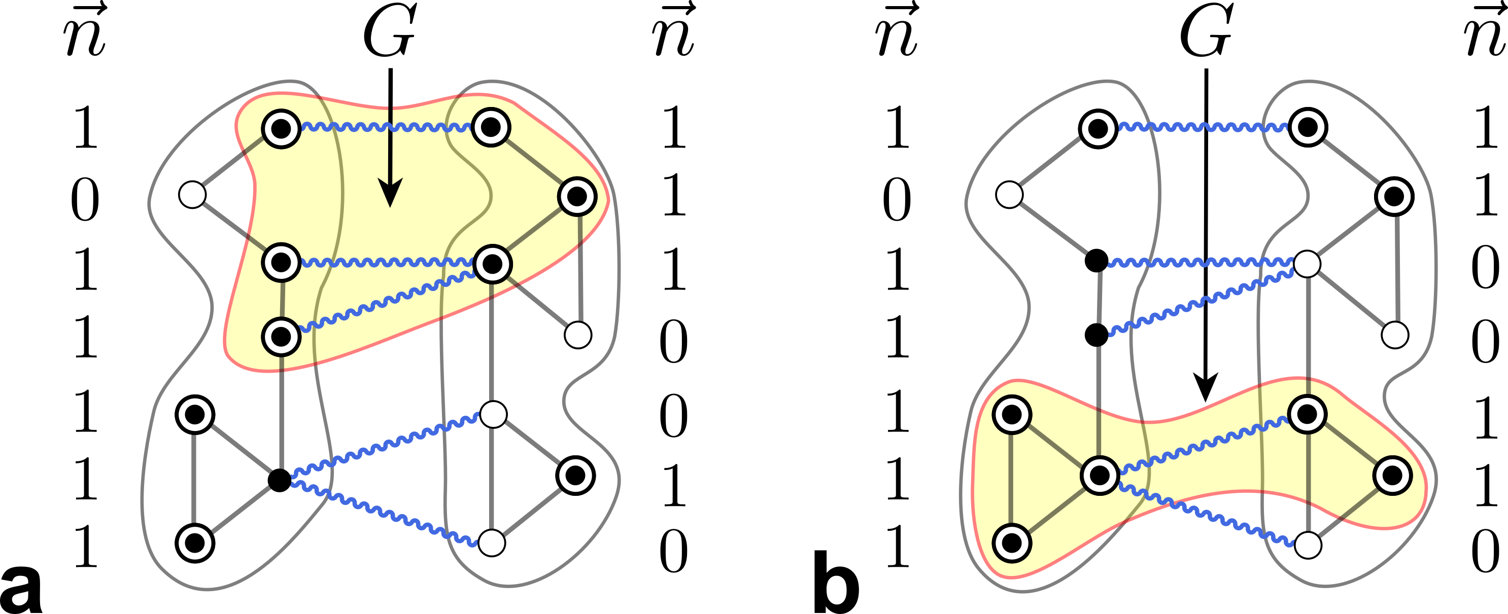
Figure 1: (Color online) Robust interdependent 2-NoN. Intra-module links (black) represent connectivity, while inter-module links (wiggly blue lines) express mutual dependencies. The occupation variable $n_{i}$ specifies whether a node is present ($n_{i}=1$) or removed ($n_{i}=0$). The activation state $\sigma_{i}$, defined through inter-module dependencies, indicates whether a node is activated ($\sigma_{i}=1$) or inactivated ($\sigma_{i}=0$). Nodes can be activated even if they do not belong to the giant connected activated component $G$. Note also that the configuration of occupation variables $\vec{n}$ is identical for the module on the left in a and b. Legend: $\sigma_{i}=1$; $\bullet$ $n_{i}=1$, $\sigma_{i}=0$; $\circ$ $n_{i}=0$, $\sigma_{i}=0$.

Definition of control intra-modular links.— Consider $N$ nodes in a NoN composed of several interdependent modules (Fig. 1). We distinguish the roles of intra-module links connecting nodes within a module, and inter-module dependency links (corresponding to control links in the brain gallos ; saulo ), connecting nodes across modules: the former (intra-links) only represent whether or not two nodes are connected, the latter (inter-links) express mutual control. Every node $i$ has $k^{\rm in}_{i}$ intra-module links, referred to as node $i$’s in-degree, and $k^{\rm out}_{i}$ inter-module connections, referred to as $i$’s out-degree.

Each node can be present or removed, and, if present, it can be activated or inactivated. We introduce the binary occupation variable $n_{i}=1,0$ to specify whether node $i$ is present $(n_{i}=1)$ or removed $(n_{i}=0)$. By virtue of inter-module dependencies, the functioning of a node in one module depends on the functioning of nodes in other modules. In order to conceptualize this form of control, we introduce the activation state $\sigma_{i}$, taking values $\sigma_{i}=1$ if node $i$ is activated and $\sigma_{i}=0$ if not. A node $i$ with one or more inter-module dependency/control connections $(k^{\rm out}_{i}\geq 1)$ is activated $(\sigma_{i}=1)$ if and only if it is present $(n_{i}=1)$ and at least one of its out-neighbors $j$ is also present $(n_{j}=1)$, otherwise it is not activated $(\sigma_{i}=0)$. In other words, a node with one or several inter-module dependencies is inactivated when the last of its out-neighbors is removed.

The rationale for this control rule is that the activation ($\sigma_{i}=\sigma_{j}=1$) of two nodes connected by, for instance, one inter-link occurs only when both nodes are occupied, $n_{i}=n_{j}=1$. If just one of them is unoccupied, let’s say $n_{j}=0$, then both nodes become inactive. Thus, $\sigma_{i}=0$ even though $n_{i}=1$, and we say that $j$ exerts a control over $i$. This rule models the way neurons control the activation of other neurons in distant brain modules via control/dependency links (fibers through the white matter) in a process known as top-down influence in sensory processing sigman . Mathematically, $\sigma_{i}$ is defined as

$$\sigma_{i}\ =\ n_{i}\bigg{[}1-\prod_{j\in\mathcal{F}(i)}(1-n_{j})\bigg{]}\,,$$ (1)

where $\mathcal{F}(i)$ denotes the set of nodes connected to $i$ via an inter-module link. Conceptually, the inter-links define a mapping from the configuration of occupation variables $\vec{n}\equiv(n_{1},...,n_{N})$ to the configuration of activated states $\vec{\sigma}\equiv(\sigma_{1},...,\sigma_{N})$, as given by Eq. (1).

Not all nodes participate in the control of other nodes via dependencies, i.e. a certain fraction of them does not establish inter-links. If a node does not have inter-module dependencies, it activates as long as it is present:

$$\sigma_{i}=n_{i}\,,\,\,\,\,\,\,\mbox{for $k^{\rm out}_{i}=0$ .}$$ (2)

Therefore, products over empty sets $\mathcal{F}({i})=\emptyset$ default to zero in Eq. (1). This last property also guarantees that we recover the single network case for vanishing inter-module connections $(\langle k^{\rm out}_{i}\rangle\rightarrow 0$), i.e. when considering the limiting case of one isolated module only.

When a fraction of nodes is removed, the NoN breaks into isolated components of activated nodes. In this work we focus on the largest (giant) mutually connected activated component $G$, which encodes global properties of the system. In contrast to previous NoN models Buldyrev2010:Cascade ; Gao2012:Interdependent , in our model a node can be activated even if it does not belong to $G$ (see Fig. 1). Indeed, the activation of a node, given by Eq. (1), is not tied to its membership in the giant component. Therefore, a node can be part of $G$ without being part of the largest connected activated component in its own module (consider for instance the top left node in Fig. 1 a). As a consequence, controlling dependencies in the NoN do not lead to cascades of failures, which ultimately explains the robustness of our NoN model. In the model of Refs. Buldyrev2010:Cascade ; Gao2012:Interdependent , on the other hand, a node can be activated (therein termed “functional”) if and only if it belongs to the largest connected component of its own module and (for the case that it has inter-module dependency links) its out-neighbors also belong to the giant component within their module. Indeed, in Refs. Buldyrev2010:Cascade ; Gao2012:Interdependent the propagation of failures is not local as in Eq. (1), implying that the failure of a single node may catastrophically destroy the NoN.

In order to quantify robustness, we measure the impact of node failures $n_{i}=0$ on the size of $G$ Buldyrev2010:Cascade ; Gao2012:Interdependent ; Bianconi2015:MutualComponent . More precisely, we calculate $G$ under typical configurations $\vec{n}$, sampled from a flat distribution with a given fraction $q\equiv 1-\sum_{i=1}^{N}n_{i}/N$ of removed nodes, and show that $G$ remains sizeable even for high values of $q$. In practice, starting from $q=0$, we compute $G(q)$ while progressively increasing the fraction $q$ of randomly removed nodes. The robustness of the NoN is then formally characterized by the critical fraction $q_{c}$, the percolation threshold, at which the giant connected activated component collapses $G(q_{c})=0$ Buldyrev2010:Cascade ; Gao2012:Interdependent . Accordingly, NoN models with high $q_{c}$ (ideally close to 1) are robust, whereas low $q_{c}$ is considered fragile. A plot of $G(q)$ for ER 2-NoN is shown in the inset of Fig. 2.

Message Passing.— The problem of calculating $G$ can be solved using a message passing approach Bianconi2015:MutualComponent ; MoMa ; Zdeborova2014:Percolation which provides exact solutions on locally tree-like NoN, containing a small number of short loops Zdeborova2014:Percolation . This includes the thermodynamic limit $(N\to\infty)$ of Erdös-Rényi and scale-free random graphs as well as the configuration model (the maximally random graphs generated from a given degree distribution), which contain loops whose typical length grows logarithmically with the system size Dorogovtsev2003 .

In principle, it works like this: each node receives messages from its neighbors containing information about their membership in $G$. Based on what they receive, the nodes then send further messages until everyone eventually agrees on who belongs to $G$. In practice, we need to derive a self-consistent system of equations that specifies for each node how the message to be sent is computed from the incoming messages Mezard2009 . To this end, we introduce two types of messages: $\rho_{i\to j}$ running along an intra-module link and $\varphi_{i\to j}$ running along an inter-module link. Formally, we denote $\rho_{i\to j}\equiv$ probability that node $i$ is connected to $G$ other than via in-neighbor $j$, and $\varphi_{i\to j}\equiv$ probability that node $i$ is connected to $G$ other than via out-neighbor $j$. The binary nature of the occupation variables and the activation states constrains the messages to take values $\rho_{i\to j},\varphi_{i\to j}\in\{0,1\}$.

A node can only send non-zero information if it is activated, hence the messages must be proportional to $\sigma_{i}$. Assuming node $i$ is activated, it can send a non-zero intra-module message $\rho_{i\to j}$ to node $j$ if and only if it receives a non-zero message by at least one of its in-neighbors other than $j$ or one of its out-neighbors. Similarly, we can consider the message $\varphi_{i\to j}$ along an inter-module link. Thus, the self-consistent system of message passing equations is given by:

$$\rho_{i\to j} =\sigma_{i}\Big{[}1-\prod_{k\in\mathcal{S}(i)\setminus j}(1-\rho_{k\to i})\prod_{k\in\mathcal{F}(i)}(1-\varphi_{k\to i})\Big{]}\ ,$$ (3)

$$\varphi_{i\to j} =\sigma_{i}\Big{[}1-\prod_{k\in\mathcal{S}(i)}(1-\rho_{k\to i})\prod_{k\in\mathcal{F}(i)\setminus j}(1-\varphi_{k\to i})\Big{]}\ ,$$ (4)

where $\mathcal{S}(i)$ denotes the set of node $i$’s intra-module nearest neighbors and $\mathcal{F}(i)$ denotes the set of $i$’s inter-module nearest neighbors. Note that products over empty sets $\mathcal{S}(i)=\emptyset$ or $\mathcal{F}(i)=\emptyset$ default to one.

In practice, the message passing equations are solved iteratively. Starting from a random initial configuration $\rho_{i\to j},\varphi_{i\to j}\in\{0,1\}$, the messages are updated until they finally converge. From the converged solutions for the messages we can then compute the marginal probability $\rho_{i}=0,1$ for each node $i$ to belong to the giant connected activated component $G$:

$$\rho_{i}\ =\ \sigma_{i}\Big{[}\hskip 1.0pt1\ -\prod_{k\in\mathcal{S}(i)}(1-\rho_{k\to i})\prod_{k\in\mathcal{F}(i)}(1-\varphi_{k\to i})\hskip 1.0pt\Big{]}\ .$$ (5)

The size of $G$, or rather the fraction of nodes belonging to $G$, can then simply be computed by summing the probability marginals $\rho_{i}$ and dividing by the system size: $G(\vec{n})=\big{(}\sum_{i=1}^{N}\rho_{i}\big{)}/N$.

Percolation Phase Diagram for ER NoN.— In what follows we derive an exact expression for the percolation threshold in Erdös-Rényi 2-NoN, defined as two randomly interconnected ER modules. Each module is an ER random graph with Poisson degree distribution, $\mathds{P}_{z}[k^{\rm in}]=e^{-z}z^{k^{\rm in}}/k^{\rm in}!$ for $k^{\rm in}\in\mathbb{N}_{0}$, where $z\equiv\langle k^{\rm in}\rangle$ denotes the average in-degree. Similarly, we consider the inter-module links to form a bipartite ER random graph with Poisson degree distribution, $\mathds{P}_{w}[k^{\rm out}]=e^{-w}w^{k^{\rm out}}/k^{\rm out}!$ for $k^{\rm out}\in\mathbb{N}_{0}$, where $w\equiv\langle k^{\rm out}\rangle$ denotes the average out-degree. The corresponding distributions for the in-/out-degree at the end of an intra-/ inter-link are given by, $\mathds{Q}_{z}[k^{\rm in}]=(k^{\rm in}\mathds{P}_{z}[k^{\rm in}]\mathds{1}_{\{k^{\rm in}>0\}})/z$ and $\mathds{Q}_{w}[k^{\rm out}]=(k^{\rm out}\mathds{P}_{w}[k^{\rm out}]\mathds{1}_{\{k^{\rm out}>0\}})/w$, for $k^{\rm in},k^{\rm out}$ in $\mathbb{N}_{0}$, where $\mathds{1}_{\{\cdot\}}$ denotes the indicator function.

The random percolation process is then defined by removing each node in the NoN independently with probability $q$, which is equivalently formulated as taking the configurations $\vec{n}=(n_{1},...,n_{N})$ at random from the binomial distribution, $\mathds{P}_{p}[\vec{n}]=\prod_{i=1}^{N}p^{n_{i}}(1-p)^{1-n_{i}}$, where $p=1-q$ denotes the occupation probability.

The probability of a node to be activated when a randomly chosen fraction $p$ of nodes in the NoN is present, $\big{\langle}\sigma_{i}\big{\rangle}_{p}=p\mathds{1}_{\{k_{i}^{\rm out}=0\}}+p\big{[}1-(1-p)^{k^{\rm out}_{i}}\big{]}\mathds{1}_{\{k_{i}^{\rm out}>0\}}$, can straightforwardly be obtained by averaging $\sigma_{i}$, given by Eq. (1), over $\mathds{P}_{p}[\vec{n}]$. The expected fraction of activated nodes $\big{\langle}\sigma_{i}\big{\rangle}_{p,w}=p\big{[}1+e^{-w}-e^{-wp}\big{]}$ is then given by averaging $\big{\langle}\sigma_{i}\big{\rangle}_{p}$ over $\mathds{P}_{w}[k^{\rm out}_{i}]$. Unlike a node’s probability to be present $\langle n_{i}\rangle_{p}=p$, the probability to be activated $\langle\sigma_{i}\rangle_{p}$ is therefore highly dependent on the node’s out-degree $k^{\rm out}_{i}$. In other words, the deactivations are highly degree dependent, even if the fraction $q$ of nodes to be removed from the NoN is chosen randomly!

To compute the expectation of messages within the ensemble of ER 2-NoN, we average the expressions for $\rho_{i\to j}$ and $\varphi_{i\to j}$, representing the converged solutions to the message passing equations, over all possible realizations of randomness inherent in the above distributions. In doing so, we must however make sure to properly account for the fact that, for nodes $i$ with inter-links ($k_{i}^{\rm out}\geq 1$), the binary occupation variable $n_{i}$ shows up more than once within the entire system of message passing equations, due to the activation rule for $\sigma_{i}$. Indeed, since the occupation variable is a binary number $n_{i}\in\{0,1\}$, powers of $n_{i}^{k}=n_{i}$ for each exponent $k\in\mathbb{N^{+}}$ and therefore the self-consistency is not affected by the existence of multiple $n_{i}$ per node. Yet, when naively averaging with the distribution of configurations, we would incorrectly obtain $n_{i}^{k}\overset{\mathds{P}_{p}}{\longrightarrow}p^{k}$ instead of $n_{i}^{k}\overset{\mathds{P}_{p}}{\longrightarrow}p$, without properly accounting for the binary nature of the occupation variable across the entire system of equations.

Specifically, when inserting the expression for the message $\varphi_{k\to i}$, determined by Eq. (4), into the expression for $\rho_{i\to j}$, given by Eq. (3), then the activation state $\sigma_{k}=n_{k}[1-(1-n_{i})\prod_{\ell\in\mathcal{F}(k)\setminus i}(1-n_{\ell})\big{]}$ (within $\varphi_{k\to i}$) reduces to $n_{k}$, since $n_{i}(1-n_{i})=0$ for binomial variables. In other words, we need to replace $\sigma_{k}$ ($\sigma_{i}$) with $n_{k}$ ($n_{i}$) within the expression for $\varphi_{k\to i}$ ($\varphi_{i\to j}$, Eq. (4)).

Thus, the modified message passing equations we need to average read:

$$\rho_{i\to j} =\sigma_{i}\Big{[}1-\prod_{k\in\mathcal{S}(i)\setminus j}(1-\rho_{k\to i})\prod_{k\in\mathcal{F}(i)}(1-\varphi_{k\to i})\Big{]}\ ,$$ (6)

$$\varphi_{i\to j} =n_{i}\Big{[}1-\prod_{k\in\mathcal{S}(i)}(1-\rho_{k\to i})\prod_{k\in\mathcal{F}(i)\setminus j}(1-\varphi_{k\to i})\Big{]}\ .$$

In practice, we expand $\rho_{i\to j}$, given by Eq. (6), and perform the averaging separately for each term:

$$\rho_{i\to j} =n_{i}\Big{[}1-\prod_{k\in\mathcal{S}(i)\setminus j}(1-\rho_{k\to i})\Big{]}\mathds{1}_{\{k^{\rm out}_{i}=0\}}$$ (7)

$$+\sigma_{i}\Big{[}1-\prod_{k\in\mathcal{S}(i)\setminus j}(1-\rho_{k\to i})\prod_{k\in\mathcal{F}(i)}(1-\varphi_{k\to i})\Big{]}\mathds{1}_{\{k^{\rm out}_{i}>0\}}\ .$$

The only non-trivial average involves the following expression:

$$\Big{\langle}\sigma_{i}\prod_{k\in\mathcal{S}(i)\setminus j}(1-\rho_{k\to i})\prod_{k\in\mathcal{F}(i)}(1-\varphi_{k\to i})\,\mathds{1}_{\{k^{\rm out}_{i}>0\}}\Big{\rangle}$$ (8)

$$=\Big{\langle}n_{i}\prod_{k\in\mathcal{S}(i)\setminus j}(1-\rho_{k\to i})\Big{[}\prod_{k\in\mathcal{F}(i)}(1-\varphi_{k\to i})$$

$$-\ \prod_{k\in\mathcal{F}(i)}(1-n_{k})(1-\varphi_{k\to i})\Big{]}\mathds{1}_{\{k^{\rm out}_{i}>0\}}\Big{\rangle}\ ,$$

where we have to account for the fact that $(1-n_{k})(1-\varphi_{k\to i})=(1-n_{k})$. The final expression for the average intra-module message $\rho$ reads:

$$\rho=p\big{[}1+e^{-w}-e^{-wp}-e^{-z\rho-w}+e^{-z\rho-wp}-e^{-z\rho-w\varphi}\big{]}.$$ (9)

Averaging the modified inter-link message $\varphi_{i\to j}$, given by Eq. (6), over all possible realizations of randomness inherent in the percolation process yields:

$$\varphi\ =\ p\,\big{[}\,1-e^{-z\,\rho\,-w\,\varphi}\,\big{]}\ .$$ (10)

The percolation threshold $p_{c}=1-q_{c}$ of the ER 2-NoN can now be found by evaluating the leading eigenvalue determining the stability of the fixed point solution $\{\rho=\varphi=0\}$ to the averaged modified message passing equations Zdeborova2014:Percolation :

$$\left.\left(\begin{array}[]{cc}\frac{\partial\rho}{\partial\rho}&\frac{\partial\varphi}{\partial\rho}\\ \frac{\partial\rho}{\partial\varphi}&\frac{\partial\varphi}{\partial\varphi}\end{array}\right)\right|_{\{\rho=\varphi=0\}}=\left(\begin{array}[]{cc}pz\big{[}1+e^{-w}-e^{-wp}\big{]}&pz\\ pw&pw\end{array}\right)_{.}$$ (11)

The corresponding eigenvalues can readily be obtained as

$$\lambda_{\pm}=\frac{p}{2}\Big{[}z[1+f]+w\pm\sqrt{z^{2}[1+f]^{2}+2zw[1-f]+w^{2}}\Big{]}$$ (12)

where we define $f(p)\equiv e^{-w}-e^{-wp}$. Formally, the fixed point solution $\{\rho=\varphi=0\}$ is stable if and only if $\lambda_{+}\leq 1$ MoMa ; Zdeborova2014:Percolation . The implicit function theorem then allows us to obtain the percolation threshold $p_{c}=1-q_{c}$ by saturating the stability condition as follows:

$$\lambda_{+}\hskip 1.0pt(\hskip 1.0ptp,\hskip 1.0ptz,\hskip 1.0ptw\hskip 1.0pt)\ =\ 1\hskip 5.69046pt\rightarrow\,\,\ p_{c}\hskip 1.0pt(\hskip 1.0ptz,\hskip 1.0ptw\hskip 1.0pt)\ .$$ (13)

Results for $q_{c}(z,w)=1-p_{c}(z,w)$ in ER 2-NoN are shown in Fig. 2 and confirm the excellent agreement between direct simulations of the random percolation process on synthetic NoN and the theoretical percolation threshold calculated from Eq. (13). The numerically measured percolation thresholds, $q_{c}^{\rm num}(z,w)$, were obtained at the peak of the second largest activated component (Fig. 2  Inset), measured relative to the fraction of randomly removed nodes in synthetic ER 2-NoN. The analytical prediction of the percolation threshold, $q_{c}^{\rm analytic}(z,w)$, was obtained from the numerical solution of Eq. (13).

The large values of $q_{c}$ in the percolation phase diagram confirm that the NoN is very robust with respect to random node failures. The results indicate, for instance, that a fraction of more than 70% of randomly chosen nodes in an ER 2-NoN with $\langle k^{\rm in}\rangle=4$ can be damaged without destroying the giant connected activated component $G$. Moreover, the percolation transition, separating the phases $G>0$ and $G=0$, is of second order in the robust NoN (Fig. 2  Inset).

Interestingly, the phase diagram reveals that, for a given average in-degree $z$, the NoN exhibits maximal vulnerability $q_{c}^{\rm min}(w^{*},z)=1-p_{c}^{\rm max}(w^{*},z)$ at a characteristic average out-degree $w^{*}(z)$, indicated by the dip in the percolation threshold $q_{c}$ in Fig. 2. The equation determining $w^{*}(z)$ can straightforwardly be obtained via implicit differentiation of $\lambda_{+}(p_{c},z,w)=1$, using $\partial p_{c}/\partial w\,|_{w^{*}}=0$, where $p_{c}(z,w)$ is given by the solution of Eq. (13). The corresponding curve for $q_{c}^{\rm min}(w^{*},z)$ is shown in Fig. 2. Conceptually, the dip in $q_{c}$ occurs as a consequence of the competition between dependency and redundancy effects in the NoN. Starting from vanishing inter-module connections, the critical fraction $q_{c}$, and therefore the robustness of the NoN, initially decreases slightly as the number of dependency links in the NoN is increased. However, upon further increasing the density of inter-module dependencies, the resilience of the NoN increases again with increasing redundancy among the dependency connections.

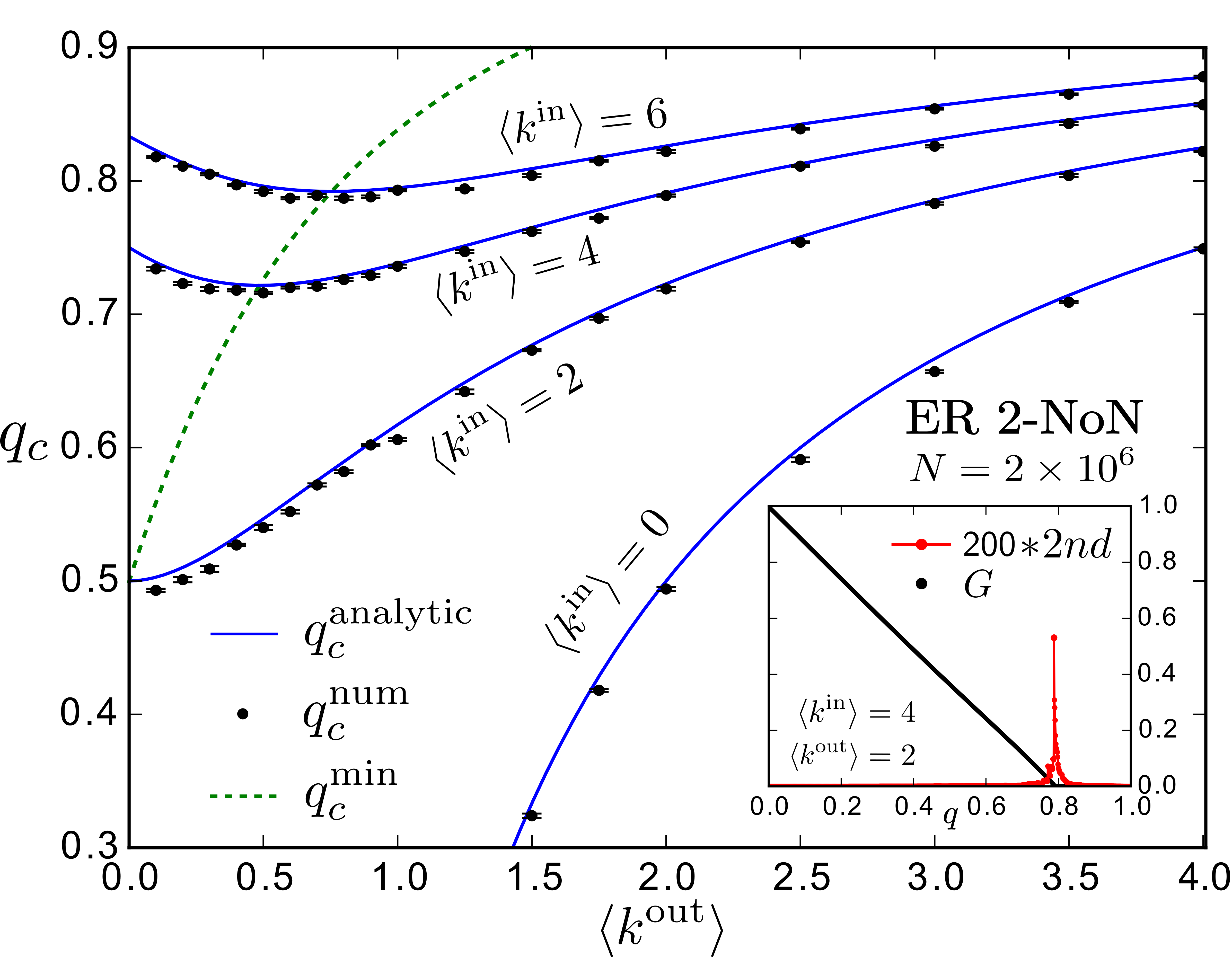
Figure 2: (Color online) Percolation phase diagram for ER 2-NoN. Blue curves show our analytical prediction of the percolation threshold, $q_{c}^{\rm analytic}$, as a function of $\langle k^{\rm out}\rangle$ for different values of $\langle k^{\rm in}\rangle=0,2,4,6$, obtained from Eq. (13). Black dots show the measured numerical percolation threshold, $q_{c}^{\rm num}$, from direct simulation of the random percolation process, obtained at the peak of the second largest connected activated component. The green dashed line indicates the maximal vulnerability $q_{c}^{\rm min}$. The percolation transition $q_{c}$ denotes the critical fraction of randomly removed nodes at which $G(q_{c})=0$ collapses. Errors are s.e.m. over 10 NoN realizations of system size $N=2\times 10^{6}$. Inset. Size of $G$ (black dots) and $200$ $*$ size of the second largest connected activated component (red dots) as a function of $q$ for an ER 2-NoN with $\langle k^{\rm in}\rangle=4$, $\langle k^{\rm out}\rangle=2$ and $N=2\times 10^{6}$. The peak is at $q_{c}^{\rm num}=0.788$.

The underlying mechanism responsible for the robustness of the NoN is best understood from the behaviour of the model in the limit $\langle k^{\rm in}\rangle\rightarrow 0$, which corresponds to a bipartite network equipped with our activation rule for $\sigma_{i}$, given by Eq. (1). The corresponding message passing equations, $\varphi_{i\to j}=\sigma_{i}\big{[}1-\prod_{k\in\mathcal{F}(i)\setminus j}(1-\varphi_{k\to i})\big{]}$, are straightforwardly obtainable from Eqs. (3)&(4), and can be seen to coincide with the usual single network message passing equations by observing that the activation state $\sigma_{i}$ can actually be replaced with the occupation variable $n_{i}$ in this case (the reason is the following: assuming node $i$ is present $(n_{i}=1)$, $\sigma_{i}=0$ implies that none of $i$’s out-neighbors is present and so none of the incoming inter-module messages can be non-zero either). This property can of course directly be obtained also from Eq. (12), which in the limit $z=0$ implies

$$\lambda_{\pm}^{z=0}=\frac{p}{2}\,\big{\{}\,w\,\pm\,\sqrt{\,w^{2}\,}\,\big{\}}\ \hskip 5.69046pt\rightarrow\,\,\ p_{c}^{z=0}=1/w\ .$$ (14)

Therefore, the functioning of dependency links is well-defined even if they connect nodes that do not belong to the giant connected activated component within each module. In the model of Refs Buldyrev2010:Cascade ; Gao2012:Interdependent , on the other hand, inter-module links only exist if they connect nodes that belong to the largest connected activated component in their own module. Hence, it is impossible to construct the NoN from below $p_{c}$ (or above $q_{c}$) using dependency links. In the present robust model, we can construct the links even if the nodes are not in $G$, allowing us to build the NoN from below $p_{c}$ using dependency connections. Thus, the transition is well-defined from above and below the percolation threshold.

In conclusion, we have seen that the robustness in NoN can be understood to emerge if dependency links do not need to be part of the giant connected activated component $G$ for their proper functioning. In contrast to previously existing models of interdependent networks Buldyrev2010:Cascade ; Gao2012:Interdependent , dependencies in the robust NoN do not lead to cascades of failures. The key point in our model is that a node can be activated even if it does not belong to $G$. An example of the structure of NoN where the model applies is that of the brain gallos ; saulo ; preprint ; sigman . While in Ref. saulo we have shown that the model of Buldyrev2010:Cascade becomes robust when correlations in the dependencies are considered, here we show that a local activation rule Eq. (1) akin to brain control between modules defines a novel model of NoN which is robust even without correlations. The effect of degree correlations on the robustness of the NoN is to be investigated saulo . The model is straightforwardly generalizable also to directed links and to dependency connections not restricted to be only across modules, but also inside each module.

Acknowledgment. We acknowledge funding from NSF PHY-1305476, NIH-NIGMS 1R21GM107641, NSF-IIS 1515022 and Army Research Laboratory Cooperative Agreement Number W911NF-09-2-0053 (the ARL Network Science CTA).

References

- (1) M. E. J. Newman, Networks: An Introduction (Oxford University Press, USA, 2010).
- (2) S. V. Buldyrev, R. Parshani, G. Paul, H. E. Stanley, and S. Havlin, Nature 464, 1025 (2010).
- (3) J. Gao, S. V. Buldyrev, H. E. Stanley, and S. Havlin, Nature Phys. 8, 40 (2012).
- (4) G. Bianconi, S. N. Dorogovtsev, and J. F. F. Mendes, Phys. Rev. E 91, 012804 (2015).
- (5) R. Parshani, S. V. Buldyrev, and S. Havlin, Phys. Rev. E 105, 048701 (2010).
- (6) S. D. S. Reis, Y. Hu, A. Babino, J. S. Andrade Jr, S. Canals, M. Sigman, and H. A. Makse, Nature Phys. 10, 762 (2014).
- (7) F. Morone, K. Roth, B. Min, H. E. Stanley, and H. A. Makse, (submitted, 2016) http://bit.ly/1YuumcS
- (8) L. K. Gallos, H. A. Makse, and M. Sigman, Proc. Natl. Acad. Sci. USA 109 2825 (2012).
- (9) C. D. Gilbert and M. Sigman, Neuron 54, 677 (2007).
- (10) F. Morone, and H. A. Makse, Nature 524, 65 (2015).
- (11) B. Karrer, M. E. J. Newman, and L. Zdeborová, Phys. Rev. Lett. 113, 208702 (2014).
- (12) S. N. Dorogovtsev, J. F. F. Mendes, and A. N. Samukhin, Nucl. Phys. B 653, 307 (2003).
- (13) M. Mézard, and A. Montanari, Information, Physics, and Computation (Oxford University Press, USA, 2009).