Household Income Distribution in the USA

In this article we present an alternative model for the distribution of household incomes in the United States. We provide arguments from two differing perspectives which both yield the proposed income distribution curve, and then fit this curve to empirical data on household income distribution obtained from the United States Census Bureau.

1 Introduction

Understanding the statistical nature of income and wealth distributions has been a long-standing problem in the field of economics. Income is based on the concept of money. Although related to each other, the two concepts—income and wealth—are not interchangeable. In this article, we are interested in the study of income distributions in the USA.

One of the earliest and most notable attempts at understanding wealth—the separation from income was fuzzier then—was pioneered by Pareto [32]. Pareto realized that the density $\rho(w)$ of people per unit wealth $w$, when $w$ is a relative large number, follows a simple power law

$$\rho(w)\propto{1\over w^{\alpha+1}}.$$

From his data, Pareto estimated the exponent $\alpha$ to be about $3/2$. Today the above relation is known as Pareto’s law and the exponent $\alpha$ as the Pareto exponent. Since the time of Pareto, many improvements and alternative approaches have been proposed as well as extensive discussions on income and wealth inequality. (Among a huge list, perhaps references [1, 2, 8, 29] is a good starting point.)

Gibrat [26] was actually the first to look at the income of the middle-range people and conclude that that the distribution follows a log-normal curve. The Pareto and Gibrat conclusions have been derived mathematically and studied more carefully by many mathematicians and physicists (for example, [12, 25, 27, 34, 35]). They have been at the core of the most of the traditional models of income which treat individual income as a stochastic variable and from which the income distribution is derived based on an analysis of the behavior at low and high income values and, eventually, interpolating between between the two ranges. It is now known that the Kesten stochastic process, defined by the recursion $x_{i+1}=a_{i}\,x_{i}+b_{i}$, where $a_{i}$, $b_{i}$ are positive random numbers can produce a power law in the tail. The role of the $b_{i}$ term is of paramount importance; it was quickly understood to be necessary in order to generate the power law. Without it, the distribution of $x_{i}$ is log-normal.

More recently, with the explosion of econophysics, empirical studies of income distributions have been carried out but many physicists who have used ideas from physics to analyze and interpret the data. Among them are those by Dragulescu and Yakovenko [19, 20] for UK and USA, by Fujiwara et al. [24] for Japan, by Nirei and Souma [30] for US and Japan, by Ferrero [22, 23] for Japan, UK, New Zealand and Argentina. Also, Clementi and collaborators have looked at the power tails in income distributions for Italy, Germany, UK and USA [13, 14, 16].

The knowledge of a population’s distribution of income is an important piece of information to understand the economic health of a nation through an objective quantitative tool. It also provides one with the means of estimating income inequality, and can reveal information on the existence of economic classes within a society. Developing a theoretical model of society to predict the form of income distributions is then an important step in accurately determining the aforementioned data which can then be used as a guide to help build a secure and more stable economic landscape.

Excluding the high income range, Dragulescu and Yakovenko have argued that there is evidence for an exponential Boltzmann distribution of income for single earner households [19]. The idea and data are reviewed in [21, 37]. Motivated by the belief that economic markets and systems that are comprised by a large number of interacting economic agents must be describable by the the same statistical laws obeyed by physical systems composed of interacting particles, physicists have created many kinetic models of wealth and income. In such models, agents interact via an exchange process wherein they exchange some amount of their wealth in a process which is analogous to the exchange of momentum between gas particles. A sample of papers of such models are [4, 6, 7, 10, 11, 15, 18, 33]; the books [9, 31] summarize very nicely the kinetic exchange models created by physicists to describe income and wealth distributions (where additional related references may also be found). Inspired by this trend, in the present article, we propose a model for the income distribution of households in the United States. Our model is developed based on analogy with physical systems — in particular, the blackbody radiation [28] — and provides an excellent fit to US Census data of income distributions. This approach of transferring ideas from physical systems to economic systems (when and where possible) grants us the advantage of accessing the large body of mathematical techniques developed in statistical physics while simultaneously providing a clear interpretation of the parameters involved in our system.

2 The Model of Income Distribution

Consider all possible income states of an economic agent. It is immediate that they constitute a discrete and, in principle, infinite set. Let $s_{1},s_{2},s_{3},\dots$ be these states and $r_{1}<r_{2}<r_{3}<\dots$ respectively be the agent’s income in these states. We also assume that the values $r_{1},r_{2},\dots$ are time-independent.

Now imagine an economic society made of $N$ agents. This society is described by its own states of income $S_{1},S_{2},S_{3},\dots$ which can be related to the states of a single agent as follows. Let $n_{i}$ agents having income $r_{i}$, $i=1,2,\dots$. We will call the $n_{i}$ the occupation number. Obviously,

$$N=\sum_{i}n_{i}.$$

The total income of the society is

$$R=\sum_{i}n_{i}\,r_{i},$$

Even for an isolated society, the numbers $N$ and $R$ do not have to be fixed. Besides human births and deaths, a developed economic society allows the creation of corporations which can have income. However, the numbers $N$ and $R$ are not crucial. The states $S_{\alpha}$ of the society are characterized by the collection of the occupation numbers $n_{1},n_{2},n_{3},\dots$.

Method 1

Consider the states $s_{m}$ and $s_{p}$ of a single economic agent with income values $r_{m}<r_{p}$. Let their occupation numbers for the society be $n_{m}$ and $n_{p}$ respectively. It is possible that some agents in state $s_{p}$ lose some of their income without any particular financial reason and drop in state $s_{m}$. For example farmers may see their crops destroyed by weather conditions and hence they will not be able to sell them to get income. ‘Weather conditions’ have nothing to do with established financial activities, so we consider them ‘no particular financial reason’. Such activities which create losses without financial reasons, we call spontaneous drops. The probability for a spontaneous drop to happen, during an infinitesimal time interval $dt$, is

$$dP(p\to m)=A_{m}^{p}\,dt,$$

where $A_{m}^{p}$ is some coefficient.

On the other hand, we can have agents who transition from one state to another because of financial activities. For example, an employer can hire a number of agents to work for him. When he pays the employees, his income decreases and the income of each of the employees increases. Such income changes which happen under the action of a financial activity, we call stimulated drops if the income decreased or stimulated raises if the income increased. The probability for a stimulated drop to happen, during an infinitesimal time interval $dt$, is

$$dP(p\to m)=B_{m}^{p}\,\rho_{p}\,dt,$$

where $B_{m}^{p}$ is some coefficient,

$$\rho(r)={dn\over dr}.$$

is the income distribution density — density of the number of agents per income and $\rho_{p}$ is a shorthand notation for $\rho(r_{p})$. The determination of the density $\rho(r)$ is the focus of the current paper.

Similarly, for a stimulated raise, we have

$$dP(p\leftarrow m)=B^{m}_{p}\,\rho_{m}\,dt,$$

where $B_{p}^{m}$ is yet another coefficient. Notice that, in the above discussion, we have excluded spontaneous raises. No agent can enjoy an increase in income without a particular financial reason.

From the above discussion, we conclude that the total probability for an income drop $p\to m$ is

$$dP_{\text{total}}(p\to m)=(A_{m}^{p}+B_{m}^{p}\,\rho_{p})\,dt.$$

The corresponding population change is

$$dn(p\to m)=n_{p}(A_{m}^{p}+B_{m}^{p}\,\rho_{p})\,dt.$$

For the raise, the corresponding population change is

$$dn(p\leftarrow m)=n_{m}\,B^{m}_{p}\,\rho_{m}\,dt.$$

For a society in equilibrium, the occupation numbers remain more or less fixed. Hence

$$n_{p}(A_{m}^{p}+B_{m}^{p}\,\rho_{p})\,dt=n_{m}\,B^{m}_{p}\,\rho_{m}\,dt.$$

At the same time, for large populations the occupation numbers follow the Boltzmann distribution[28, 36, 37]:

$$n_{p}={Ng_{p}\over Z}\,e^{-\beta r_{p}},\quad n_{m}={Ng_{m}\over Z}\,e^{-\beta r_{m}},$$

where $\beta$ is the inverse temperature (a measure of the average income), $Z$ a normalization constant (known as partition function),

$$Z=\sum_{p}g_{p}\,e^{-\beta r_{p}},$$

and $g_{p},g_{m}$ constants which take into account possible degeneracies in the states of a single agent. So, finally the equilibrium condition is:

$$g_{p}\,e^{-\beta r_{p}}(A_{m}^{p}+B_{m}^{p}\,\rho_{p})=g_{m}\,e^{-\beta r_{m}}\,B^{m}_{p}\,\rho_{m}.$$

This relation is true for any income density $\rho$. In particular, a society in which the average income is infinite: $\rho\to+\infty$ and $\beta\to 0$. Hence,

$$g_{p}B_{m}^{p}=g_{m}B^{m}_{p}.$$

Now, let’s take two successive states $p=m+1$. Hence $r_{m+1}-r_{m}=r$ and $\rho_{m+1}=\rho_{m}=\rho(r)$. Then

$$\rho(r)={C(r)\over e^{\beta r}-1},$$

where $C(r)=A_{m}^{m+1}/B_{m}^{m+1}$.

The ratio $A_{m}^{p}/B_{m}^{p}$ for any income states $p$ and $m$ should be computed through a model based on socio-economic ideas and actual data. We have constructed no such model. However, it seems natural to assume that the ratio in the income density has a simple power dependence, that is

$$C(r)=c\,r^{\alpha},$$

where $\alpha$ and $c$ some constants. We have thus concluded that the income density of a society should be given by a function of the form

$$\rho(r)={c\,r^{\alpha}\over e^{\beta r}-1}.$$ (1)

Method 2

The partition function for the society is

$$Z_{\text{society}}=\sum_{\alpha}g_{\alpha}\,e^{-\beta R_{\alpha}}~{}.$$

Any state of income of ths society is characterized by the occupation numbers $n_{1},n_{2},\dots$ each of which takes all values 0, 1, 2, …Hence

$$Z_{\text{society}}(\beta)=\sum_{\alpha}g_{\alpha}\,e^{-\beta R_{\alpha}} = \sum_{n_{1}=0}^{\infty}e^{-\beta r_{1}n_{1}}\,\sum_{n_{2}=0}^{\infty}e^{-\beta r_{2}n_{2}}\dots$$

$$= \prod_{i=1}^{\infty}{1\over 1-e^{-\beta r_{i}}}.$$

The average occupation number $n_{1}$ is

$$\overline{n}_{1} = \sum_{n_{1}=0}^{\infty}n_{1}\,e^{-\beta r_{1}n_{1}}\,\sum_{n_{2}=0}^{\infty}e^{-\beta r_{2}n_{2}}\cdots$$

$$= -{1\over\beta}{\partial\over\partial r_{1}}\sum_{n_{1}=0}^{\infty}e^{-\beta r_{1}n_{1}}\,\sum_{n_{2}=0}^{\infty}e^{-\beta r_{2}n_{2}}\dots$$

$$= {1\over e^{\beta r_{1}}-1},$$

and similarly for any other $\overline{n}_{i}$.

The density $\rho(r)$ is then equal to

$$\rho(r)=\overline{n}(r)\,g(r)={g(r)\over e^{\beta r}-1},$$

where $g(r)$ is the degeneracy at value $r$. Again, this function must be constructed as a result of a socio-economic model. This can be a very complicated task and here we assume, similarly to the previous approach, that it is a simple power function:

$$g(r)=c\,r^{\alpha},$$

with $c$ and $\alpha$ constants to be computed. We thus arrive at the same density function (1).

Actual Density for USA

Comparison with real data points out that $\alpha=3/2$ (see Section 3). Hence,

$$\rho(r)={c\,r^{3/2}\over e^{\beta r}-1}.$$ (2)

Obviously the number of economic agents is the integral of the density over all possible values of income:

$$N=\int_{0}^{+\infty}\rho(r)\,dr={c\over\beta^{5/2}}\,\int_{0}^{+\infty}{x^{3/2}\over e^{x}-1}dx.$$

Also, the income $R$ of the society is

$$R=\int_{0}^{+\infty}r\,\rho(r)\,dr={c\over\beta^{7/2}}\,\int_{0}^{+\infty}{x^{5/2}\over e^{x}-1}dx.$$

Let

$$I(\alpha)=\int_{0}^{+\infty}{x^{\alpha}\over e^{x}-1}dx.$$

This integral is known to be related to the $\zeta$-function:

$$I(\alpha)=\Gamma(\alpha+1)\,\zeta(\alpha+1)~{}.$$

Hence in our case,

$$N={3c\sqrt{\pi}\over 4\beta^{5/2}}\,\zeta(5/2)~{},$$

and

$$R={15c\sqrt{\pi}\over 8\beta^{7/2}}\,\zeta(7/2)~{},$$

since $\Gamma(5/2)=3\sqrt{\pi}/4$ and $\Gamma(7/2)=(5/2)\cdot\Gamma(5/2)$ . Writing the last results in the form

$${1\over\beta}=\text{const.}\,N^{2/5}~{},$$

and

$$R=\text{const.}\,N\,{1\over\beta}~{},$$

we see that the average income per individual scales with the population as a power law while the income of the society is proportional to its population.

3 Validation of the Model

The data used to validate the proposed model — equation (1) — were household income data [39] obtained from the US Census Bureau [38]. Incomes ranged up to $100,000 for years 1994 – 2008 and up to $200,000 for years 2009 – 2013. For each year, the total number of reported household incomes was rescaled to unity for ease of comparison across years. In other words,

$$\int_{0}^{+\infty}\rho\,dr=1.$$

In the graphs of Figure 1, this amounts to divide the population numbers for each income bracket by the total number of households.

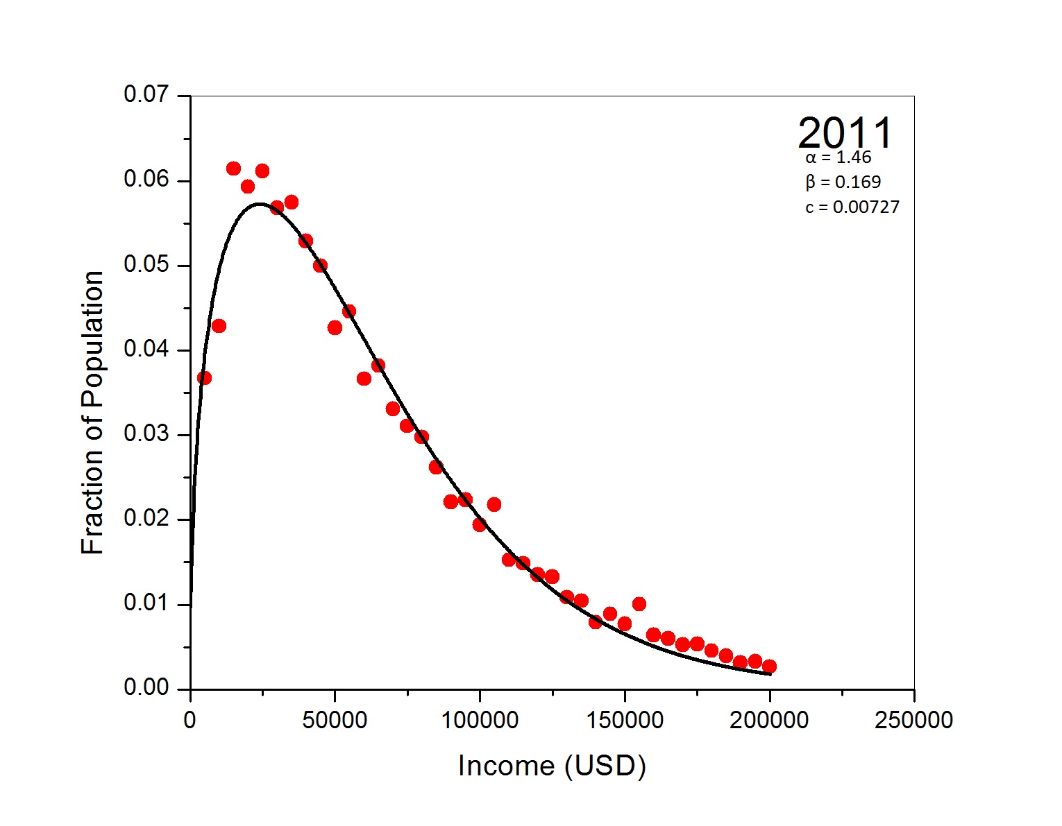
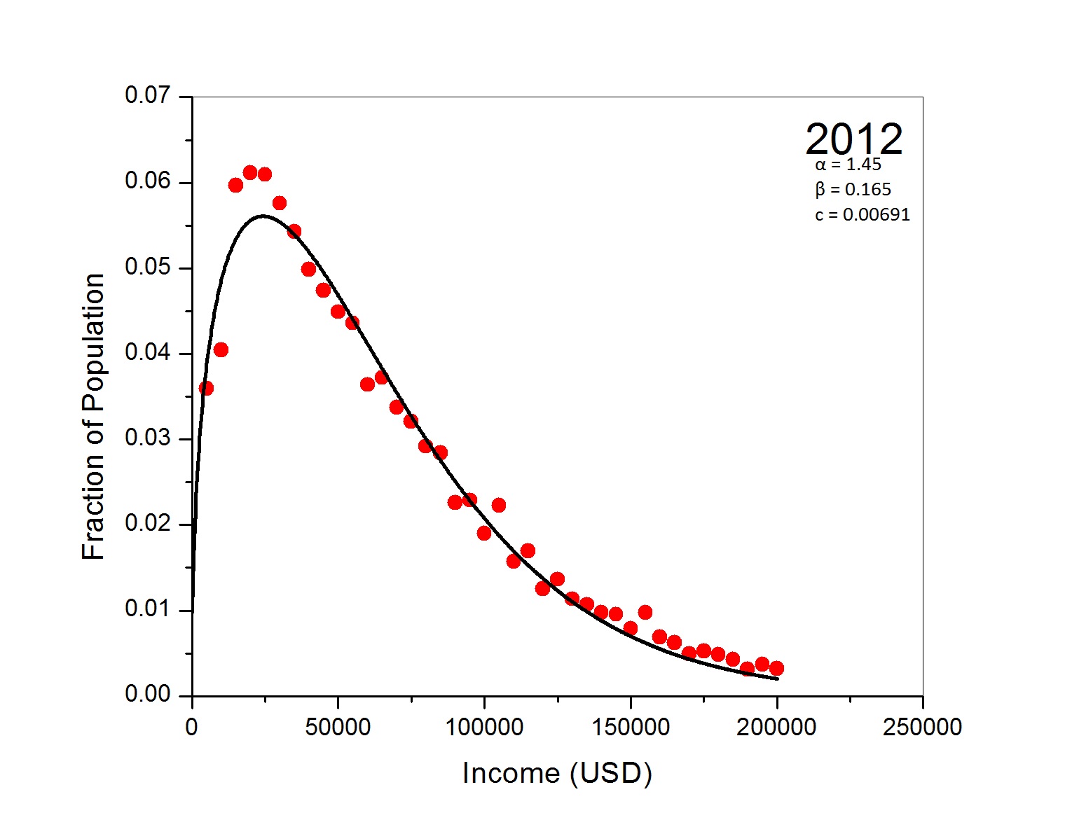
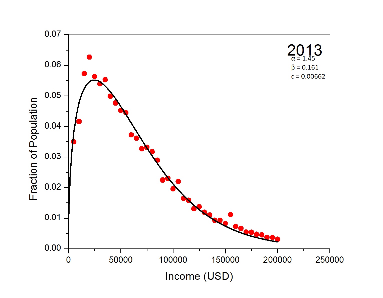
Figure 1: Plot of the density function $\rho(r)$ for the years 2009–2013.

To avoid overpopulating the article with many similar graphs, we have given the income density function $\rho(r)$ for five years, from 2009 through 2013. The data agree with the curve given by equation (1) with the earliest and latest years giving the best fits. It is worthwhile to note that the latest years have an impressive agreement with the theoretical model. In the years omitted, the data appear more scattered as we move closer to the recession period. Perhaps this behavior of income can be used to predict when we move towards a recession with a lead time of a few years. However, it is not known to us how US Census made the set of data, so some caution should be exercised for its interpretation.

From the fitting of the actual data, we can extract the values of the constants $c,\beta,\alpha$. In Figure 2 we give the values of $\alpha$ and $\beta$ over the period 1994 – 2013 and in Figure 3 the values of $c$ and $N$ over the same period.

Figure 2: Plots of the constants $\alpha$ and $\beta$ for the period 1994–2013.

As a result of the fitting, some very interesting and surprising features emerge and are worth noting. The exponent $\alpha$, although it fluctuates slightly, appears to do so around the value 3/2. For the parameters $N$, $\beta$ and $c$, there is an abrupt change (discontinuity) at the year 2009 which is the year of financial recovery. Notice that the number of economic agents jumps at higher values; however the average income (represented by $1/\beta$) jumps at lower values. The recession (left side of the discontinuity) however progressed smoothly with no discontinuity appearing at any particular year.

Figure 3: Plots of the constant $c$ and the population $N$ of the economic agents for the period 1994–2013.

Finally, we would like to mention that the proposed model has a coefficient of determination $R^{2}$ that is closer to 1 (perfect fit) than the popular household model given by the gamma distribution $c\,r\,e^{-\beta r}$ (See, for example, [19].) The values of $R^{2}$ for our model and the gamma model are shown in Table 1.

Year	$R^{2}$ (our model)	$R^{2}$ (gamma model)
1994	0.983036	0.977200
1995	0.986101	0.981773
1996	0.981993	0.976437
1997	0.982164	0.975105
1998	0.981842	0.974415
1999	0.983001	0.978122
2000	0.980909	0.975126
2001	0.979007	0.971966
2002	0.975130	0.966285
2003	0.976875	0.966319
2004	0.977173	0.967276
2005	0.970794	0.960924
2006	0.965006	0.958164
2007	0.961827	0.953202
2008	0.962009	0.953932
2009	0.994079	0.987708
2010	0.993583	0.982211
2011	0.993908	0.983525
2012	0.992951	0.981809
2013	0.993912	0.981772

Table 1: The coefficient of determination $R^{2}$ for our model and a popular household model given by the gamma distribution $c\,r\,e^{-\beta r}$. Our model consistently gives values closer to 1 for all years.

4 Discussion and Conclusions

In this article we have presented two arguments for obtaining a model of income distributions based on arguments similar to those for obtaining the black-body curve. For $e^{\beta r}\gg 1$, our model produces a gamma-like distribution curve

$$\rho(r)=c\,r^{\alpha}\,e^{-\beta r},$$

which is favored by various authors (for example, see [3, 9, 22, 23]). We have shown how the empirical data of a certain range of income values agrees well with the proposed model. The variation of the model parameters over the years reflects the period of economic instability that the United States experienced between 2003 and 2008. Interestingly, despite this unstable period, the exponent $\alpha$ of the model remains approximately constant over the years under consideration, equal to 3/2. The constancy of this parameter may then provide some deeper insight to the underlying behavior behind income dynamics of households in developed countries. It would be nice if a socio-economic model based on the particulars of the operation of the American society is found to explain the degeneracy $g(r)\propto r^{3/2}$ of income states. A finite discontinuity in the remaining two parameters of the model, $c$ and $\beta$, appears to locate the exact year of economic recovery, which in our case is 2009. During deteriorating economic conditions, the data points of the income distribution become more scattered although the profile of the curve remains the same. It will be quite valuable to compare our data and findings with similar data and findings of household income distributions from similarly economically developed countries, as well as from countries which are less developed and face larger economic turbulence.

Finally, we would like to point out the following fact: It is true that in economics and finance, there is a large number of parameters which appear to allow many different models to be constructed. However, relative good agreement with data is not automatic unless the underlying assumptions capture some of the characteristics of the dynamics. We thus hope that our model does contain some elements of truth which time will eventually verify.

References

- [1] A. B. Atkinson and F. Bourguignon, Handbook of Income Distribution, Volume 1, Elsevier, (Amsterdam, The Netherlands 2000).
- [2] A. B. Atkinson and F. Bourguignon, Handbook of Income Distribution, Volume 2, Elsevier, (Amsterdam, The Netherlands 2015).
- [3] J. Angle, The Inequality Process as a Wealth Maximizing Process, Physica A 367 (2006) 388.
- [4] A. Banerjee, V. Yakovenko, Universal patterns of inequality, New J. Phys. 12 (2010) 075032.
- [5] A. Banerjee, V.M. Yakovenko, T. Di Matteo, A study of the personal income distribution in Australia. Physica A 370 (2006) 54.
- [6] F. Bassetti, G. Toscani, Explicit equilibria in a kinetic model of gambling, Phys. Rev. E 81 (2010) 066115.
- [7] A. Chakraborti and B. K. Chakrabarti, Statistical mechanics of money: How saving propensity affects its distribution, Eur. Phys. J. B 17 (2000) 167.
- [8] B. K. Chakrabarti, A. Chakraborti and A. Chatterjee, editors, Econophysics and Sociophysics: Trends and Perspectives, Wiley-VCH 2006, Weinheim, Germany.
- [9] B.K. Chakrabarti, A. Chakraborti, S.R. Chakravarty, A. Chatterjee, Econophysics of Income and Wealth Distributions, Cambridge University Press 2013, Cambridge, UK.
- [10] A. Chatterjee, B.K. Chakrabarti, S.S. Manna, Pareto law in a kinetic model of market with random saving propensity, Physica A 335 (2004) 155.
- [11] A. Chatterjee, B.K. Chakrabarti, Kinetic exchange models for income and wealth distributions, Eur. Phys. J. B 60 (2007) 135.
- [12] D. Champernowne, A Model of Income Distribution, Economic Journal 63 (1953) 318.
- [13] F. Clementi, M. Gallegati, Power law tails in the Italian personal income distribution, Physica A 350 (2005) 427.
- [14] F. Clementi, M. Gallegati, Pareto’s law of income distribution: evidence for Germany, the United Kingdom, the United States, pp 3–14 in [17].
- [15] F. Clementi, M. Gallegati, and G. Kaniadakis, -generalized statistics in personal income distribution, Eur. Phys. J. B 57 (2007) 187.
- [16] F. Clementi, T. Di Matteo, M. Gallegati, The power-law tail exponent of income distributions, Physica A 370 (2006) 49.
- [17] A. Chatterjee, S. Yarlagadda and B. K. Chakrabarti, editors, Econophysics of Wealth Distributions, (Springer, Milan 2005).
- [18] S. Cordier, L. Pareschi, and G. Toscani, On a kinetic model for a simple market economy, J. Stat. Phys., 120 (2005) 253.
- [19] A. A. Dragulescu and V. M. Yakovenko, Evidence for the exponential distribution of income in the USA, Eur. J. Phys. B 20 (2001) 585.
- [20] A. A. Dragulescu and V. M. Yakovenko, Exponential and power-law probability distributions of wealth and income in the United Kingdom and the United States, Physica A 299 (2001) 213.
- [21] A. A. Dragulescu, V. M. Yakovenko, Statistical mechanics of money, income, and wealth: a short survey, pp. 180–183 in Modeling of Complex Systems: Seventh Granada Lectures, P. L. Garrido PL and J. Marro J (editors), American Institute of Physics (AIP) Conference Proceedings 661, New York.
- [22] J. C. Ferrero, The Statistical Distribution of Money and the Rate of Money Transference, Physica A 341 (2004) 575.
- [23] J. C. Ferrero, The Monomodal, Polymodal, Equilibrium and Nonequilibrium Distribution of Money, pp. 159–167 in [17].
- [24] Y. Fujiwara, W. Souma, H. Aoyama, T. Kaizoji, and M. Aoki, Growth and fluctuations of personal income, Physica A: Statistical Mechanics and its Applications 321 (2003) 598.
- [25] X. Gabaix. Zipf’s Law for Cities: An Explanation, Quarterly Journal of Economics 114 (1999) 739.
- [26] R. Gibrat, Les Inégalités Économiques, (Sirely, Paris, France 1931).
- [27] H. Kesten, Random Difference Equations and Renewal Theory for Products of Random Matrices, Acta Mathematica CXXXI (1973) 207.
- [28] F. Mandle, Statistical Physics, 2nd edition, John Wiley & Sons 1988.
- [29] M. Mitzenmacher, A Brief History for Generative Models for Power Law and Lognormal Distributions, Internet Mathematics 1 (2004) 226.
- [30] M. Nirei and W. Souma, A Two Factor Model of Income Distribution Dynamics, The Review of Income and Wealth 53 (2007) 440.
- [31] L. Pareschi and G. Toscani, Interacting Multiagent Systems: Kinetic Equations and Monte Carlo Methods, (Oxford University Press, Oxford 2014).
- [32] V. Pareto, Cours d’Économie Politique, (Vol. I, 1896; Vol. II, 1897, Rouge, Lausanne).
- [33] M. Patriarca, E. Heinsalu, and A. Chakraborti, Basic kinetic wealth-exchange models: Common features and open problems, Eur. Phys. J. B 73 (2010) 145.
- [34] H. A. Simon, On a Class of Skew Distribution Functions, Biometrika 42 (1955) 425.
- [35] D. Sornette, R. Cont, Convergent Multiplicative Processes Repelled From Zero: Power Laws and Truncated Power Laws, J. Phys. I France 7 (1997) 431.
- [36] V. M. Yakovenko, Statistical mechanics of money, Eur. Phys. J. B 729 (2000) 723.
- [37] V. M. Yakovenko and J. B. Rosser, Colloquium: Statistical mechanics of money, wealth, and income, Rev. Mod. Phys. 81 (2009) 1703.
- [38] United States Census Bureau, http://www.census.gov.
- [39] http://www.census.gov/hhes/www/income/index.html. Retrieved July 1, 2015.