Sparse Signal Detection with Compressive Measurements via Partial Support Set Estimation

Abstract

In this paper, we consider the problem of sparse signal detection based on partial support set estimation with compressive measurements in a distributed network. Multiple nodes in the network are assumed to observe sparse signals which share a common but unknown support. While in the traditional compressive sensing (CS) framework, the goal is to recover the complete sparse signal, in sparse signal detection, complete signal recovery may not be necessary to make a reliable detection decision. In particular, detection can be performed based on partially or inaccurately estimated signals which requires less computational burden than that is required for complete signal recovery. To that end, we investigate the problem of sparse signal detection based on partially estimated support set. First, we discuss how to determine the minimum fraction of the support set to be known so that a desired detection performance is achieved in a centralized setting. Second, we develop two distributed algorithms for sparse signal detection when the raw compressed observations are not available at the central fusion center. In these algorithms, the final decision statistic is computed based on locally estimated partial support sets via orthogonal matching pursuit (OMP) at individual nodes. The proposed distributed algorithms with less communication overhead are shown to provide comparable performance (sometimes better) to the centralized approach when the size of the estimated partial support set is very small.

I Introduction

Sparsity is one of the low dimensional structures exhibited in many signals of interest including audio, video and radar signals. A signal is said to be sparse if the coefficient vector, when represented in a known (orthogonal) basis, contains only a few significant elements. Sparsity has been exploited in signal processing and approximation theory for tasks such as compression, denoising, model selection, and image processing [1] for a long time. The problem of sparse signal recovery has attracted much attention in the recent literature with advancements of the theory of compressive sensing (CS). In the CS framework, a sparse signal can be reliably recovered with a small number of random projections under certain conditions [2, 3, 4, 5, 6, 7].

In addition to complete recovery, the problem of detecting signals which are sparse is important in many applications including sensor, cognitive radio, and radar networks. For this problem, complete signal recovery is not necessary to make a reliable detection decision. Theories and concepts developed in CS for sparse signal recovery have been exploited in the recent literature for signal detection problems [8, 9, 10, 11, 12, 13, 14, 15, 16, 17, 18, 19, 20, 21, 22, 23]. These works include deriving performance bounds for CS based signal detection [9, 10, 12, 13, 17, 18, 20, 21, 23], developing algorithms [8, 15, 16] and designing low dimensional projection matrices [14, 22]. While some of the work, such as [8, 9, 15, 16, 19, 20, 21] focused on sparse signal detection when the underlying subspace where the signal lies is unknown, some other works [12, 13, 14, 17, 18] considered the problem of detecting signals which are not necessarily sparse. In CS based sparse signal detection, the main objective is to utilize a small number of measurements to extract decision statistics to make a reliable detection decision. For example, in [9], the authors consider the case where an estimate of the sparse signal is obtained using some additional information to implement the matched filter for detection. In [8], the authors consider a greedy algorithm developed for sparse signal reconstruction where the detection decision is made after the maximum absolute coefficient of the partially estimated sparse signal exceeds a certain threshold. In this case, if the maximum component of the estimated signal exceeds the required threshold during an early iteration, complete signal recovery is not necessary.

Without completely reconstructing the signal, one possible way to perform reliable detection is to construct a decision statistic by estimating only a fraction of the support set of a sparse signal. Using greedy approaches as considered in [8], a partial support set can be computed with fewer number of iterations (thus less computational power and time), than that is required for complete signal recovery. Then, a decision statistic is computed based on the corresponding nonzero coefficients obtained via least squares estimation. When the requirement is to estimate only a fraction of the support, different approaches developed for partial support set estimation can be used with fewer compressive measurements [24]. On the other hand, with multiple sensors each observing sparse signals with joint sparse structures, the detection performance can be enhanced by proper fusion of partially estimated support sets at individual nodes. Motivated by these, in this paper, we investigate the problem of sparse signal detection based on partially estimated support sets with multiple sensors in centralized as well as distributed settings.

We consider a distributed network in which the sparse signals observed by multiple nodes share the same sparsity pattern. Each node makes CS based measurements. While sparse signal (or the complete support of the sparse signal) recovery with compressed measurements has been investigated quite extensively with multiple sensors with a common sparse support model [25, 26, 27, 28, 29, 30, 31, 32, 33, 34, 35, 36, 15, 37, 38], the problem of sparse signal detection with CS based measurements in a multiple sensor setting has not been investigated adequately. Recently, our work presented in [15, 16], extended the decentralized algorithms developed for joint sparsity pattern recovery based on greedy techniques to the case of sparse signal detection in a decentralized manner. In [15], a heuristic decision statistic based on support set indices estimated at multiple nodes via orthogonal matching pursuit (OMP) was computed in a decentralized manner. This approach counts the number of nodes estimating the same index at a given iteration of OMP, therefore, it is promising only when the network has sufficient number of nodes or the signal-to-noise-ratio (SNR) is relatively large. In [16], a similar approach has been considered using the subspace pursuit (SP) algorithm. The current work is different from [15, 16] in terms of the computation of decision statistics and the communication architectures used.

In this paper, we consider the problem in which the detection decision is made based on the knowledge of a partial support set. First, we discuss how to obtain the minimum fraction of the support set to make a detection decision with a desired performance level in a centralized setting. Second, we extend the OMP algorithm in centralized and distributed settings to perform joint partial support set estimation and sparse signal detection. Note that, in the centralized setting all the compressed observations are transmitted to the fusion center. In the distributed setting, two approaches are considered in which local decision statistics are computed based on partial support set estimates at the individual nodes. In the first distributed algorithm, based on independently estimated partial support sets, a local decision statistic is computed and transmitted to the fusion center. In the second approach, independently estimated partial support sets are fused at the fusion center to obtain an updated support set of larger size which are fed back to the nodes. In this case, it is possible to obtain the complete support set at the fusion center under certain conditions. Then, a decision statistic computed based on the updated support set is transmitted to the fusion center to compute the final decision statistic. The two distributed algorithms differ from each other in terms of the communication overhead required. Another interesting observation is that, under certain conditions, the two distributed algorithms (with less communication burden) perform better than the centralized algorithm which requires a higher communication burden.

Organization of the paper

The paper is organized as follows. In Section II, the sparse signal detection problem with compressive measurements in a distributed network is formulated. The minimum fraction of the support set required to be known in order to achieve a desired detection performance in a centralized setting is derived in Section III. Several practical algorithms based on OMP to perform sparse signal detection by partial support set estimation in centralized as well as in distributed settings are proposed in Section IV. In Section V, numerical results are presented to show the effectiveness of the proposed algorithms. Finally, concluding remarks are given in Section VI.

Notation

The following notation and terminology are used throughout the paper. Scalars are denoted by lower case letters and symbols; e.g., $x$ and $\alpha$. Lower case boldface letters are used to denote vectors; e.g., $\mathbf{x}$. Both upper case boldface letters and boldface symbols are used to denote matrices, e.g., $\mathbf{A}$, $\bm{\Phi}$. Matrix transpose is denoted by $\mathbf{A}^{T}$. The $l_{p}$ norm of a vector $\mathbf{x}$ is denoted by $||\mathbf{x}||_{p}$. Calligraphic letters are used to denote sets; e.g., $\mathcal{U}$. The notation $\mathcal{U}\setminus\mathcal{V}$ represents the set of elements in $\mathcal{U}$ which are not in $\mathcal{V}$ when $\mathcal{V}\subseteq\mathcal{U}$. By $\mathbf{B}(\mathcal{U})$, we denote the submatrix of $\mathbf{B}$ with columns indexed in $\mathcal{U}$. We use the notation $|.|$ to denote the absolute value of a scalar, as well as the cardinality of a set. We use $\mathbf{I}_{N}$ to denote the identity matrix of dimension $N$ (we avoid using subscript when there is no ambiguity) and $\mathbf{0}$ to denote the vector of all zeros with an appropriate dimension. The notation $\mathbf{x}\sim\mathcal{N}(\bm{\mu},\bm{\Sigma})$ denotes that the random vector $\mathbf{x}$ is multivariate Gaussian with mean vector $\bm{\mu}$ and covariance matrix $\bm{\Sigma}$. The notation $x\sim\mathcal{X}_{k}^{2}$ denotes that the random variable $x$ is distributed as a chi-squared with $k$ degrees of freedom while $x\sim\mathcal{X}_{k}^{2}(\lambda)$ denotes that $x$ has a non-central chi-squared distribution with non-centrality parameter $\lambda$.

II Sparse Signal Detection with Multiple Sensors

II-A Observation model with uncompressed data

Consider the problem of detecting unknown (deterministic) sparse signals in the presence of noise based on observations collected at multiple sensor nodes. Let there be $L$ nodes. The observation model at the $j$-th node under hypothesis $\mathcal{H}_{1}$, (the signal is present) and $\mathcal{H}_{0}$ (the signal is absent) is given by

$$\mathcal{H}_{1}:~{}\mathbf{x}_{j} = \bm{\theta}_{j}+\mathbf{v}_{j}$$

$$\mathcal{H}_{0}:~{}\mathbf{x}_{j} = \mathbf{v}_{j}$$ (1)

where $\bm{\theta}_{j}$ is the signal observed by the $j$-th node and $\mathbf{v}_{j}$ is the additive noise for $j=1,\cdots,L$. The signal $\bm{\theta}_{j}$, is assumed to be sparse in an orthonormal basis $\bm{\Psi}_{j}$ so that $\bm{\theta}_{j}=\bm{\Psi}_{j}\mathbf{s}_{j}$ where $\mathbf{s}_{j}$ is the $N\times 1$ coefficient vector with only $k\ll N$ nonzero elements. We assume that all the signals are sparse in the same basis so that $\bm{\Psi}_{j}=\bm{\Psi}$ and the coefficient vectors $\mathbf{s}_{j}$’s share the same sparse support. This particular joint sparse model is applicable in sensor networks where multiple sensors observe a signal that is sparse in the same basis, and the amplitudes of coefficients are different from each other due to different propagation conditions [39]. We further assume that the sparsity index $k$ is known in advance. Finding the sparsity index of a sparse signal and estimating the complete sparse signal (or the support) are conceptually different and there are several algorithms developed to achieve the former [40, 41]. The noise vector $\mathbf{v}_{j}$ is assumed to be Gaussian with $\mathbf{v}_{j}\sim\mathcal{N}(\mathbf{0},\sigma_{v}^{2}\mathbf{I}_{N})$ for $j=1,\cdots,L$.

II-B Compression via random projections

Now assume that the observations at each node are compressed via a low dimensional random projection matrix. The compressed measurement vector at the $j$-th node is given by

$$\mathbf{y}_{j} = \mathbf{A}_{j}\mathbf{x}_{j}$$ (2)

for $j=1,\cdots,L$ where $\mathbf{A}_{j}$ is an $M\times N$ ($M<N$) matrix. We assume that the elements of $\mathbf{A}_{j}$ are selected so that $\mathbf{A}_{j}$ is an orthoprojector; i.e., $\mathbf{A}_{j}\mathbf{A}_{j}^{T}=\mathbf{I}_{M}$. Let $\mathbf{B}_{j}=\mathbf{A}_{j}\bm{\Psi}$. When $\bm{\Psi}$ is an orthonormal basis, we have $\mathbf{B}_{j}\mathbf{B}_{j}^{T}=\mathbf{I}_{M}$ for $j=1,\cdots,L$. The goal is to decide between hypotheses $\mathcal{H}_{1}$ and $\mathcal{H}_{0}$ based on (2).

Let $\mathcal{U}$ be the set which contains the indices of locations of nonzero coefficients in $\mathbf{s}_{j}$ which is defined by $\mathcal{U}:=\{i\in\{1,\cdots,N\}~{}|~{}\mathbf{s}_{j}(i)\neq 0\}$ where $\mathbf{s}_{j}(i)$ denotes the $i$-th element of $\mathbf{s}_{j}$ for $i=1,\cdots,N$ and $j=1,\cdots,L$. Then we have $k=|\mathcal{U}|$, where $|\mathcal{U}|$ denotes the cardinality of $\mathcal{U}$. It is noted that $\mathcal{U}$ is the same for all the signals $\mathbf{s}_{j}$ since we consider the common sparse support model. Further let $\tilde{\mathbf{v}}_{j}=\mathbf{A}_{j}\mathbf{v}_{j}$ where $\tilde{\mathbf{v}}_{j}\sim\mathcal{(}\mathbf{0},\sigma_{v}^{2}\mathbf{I}_{M})$ when $\mathbf{A}\mathbf{A}^{T}=\mathbf{I}_{M}$. Then, the detection problem in the compressed domain can be expressed as:

$$\mathcal{H}_{1}:~{}\mathbf{y}_{j} = \mathbf{B}_{j}\mathbf{s}_{j}+\tilde{\mathbf{v}}_{j}$$

$$\mathcal{H}_{0}:~{}\mathbf{y}_{j} = \tilde{\mathbf{v}}_{j}$$ (3)

for $j=1,\cdots,L$.

Note 1.

It is worth noting that we consider the noiseless scenario in (2). If we consider the noisy scenario, the measurement model will be of the form $\mathbf{y}_{j}=\mathbf{A}_{j}\mathbf{x}_{j}+\mathbf{n}_{j}$ with $\mathbf{n}_{j}\sim\mathcal{N}(\mathbf{0},\sigma_{n}^{2})$, and we end up with the same detection problem as in (3) except that we will have $\tilde{\mathbf{v}}_{j}\sim(\mathbf{0},(\sigma_{v}^{2}+\sigma_{n}^{2})\mathbf{I})$. Thus, the analysis in the remainder of the paper will remain the same except that $\sigma_{v}^{2}$ will be replaced by $\sigma_{v}^{2}+\sigma_{n}^{2}$. For simplicity of presentation, we will employ the noiseless measurement model. Results for noisy measurements can be obtained by changing the value of variance.

II-C Sparse signal detection when the common support of the sparse signals is known

When $\mathcal{U}$ is exactly known, the detection problem in (3) reduces to

$$\mathcal{H}_{1}:~{}\mathbf{y}_{j} = \mathbf{B}_{j}(\mathcal{U})\mathbf{s}_{j}(\mathcal{U})+\tilde{\mathbf{v}}_{j}$$

$$\mathcal{H}_{0}:~{}\mathbf{y}_{j} = \tilde{\mathbf{v}}_{j}$$ (4)

for $j=1,\cdots,L$ where $\mathbf{B}_{j}(\mathcal{U})$ denotes the $M\times k$ submatrix of $\mathbf{B}_{j}$ in which columns are indexed by the ones in $\mathcal{U}$, and $\mathbf{s}_{j}(\mathcal{U})$ is a $k\times 1$ vector containing nonzero elements in $\mathbf{s}_{j}$ indexed by $\mathcal{U}$ for $j=1,\cdots,L$. When $\mathbf{B}_{j}(\mathcal{U})$ is known, (4) is the subspace detection problem which has been addressed previously [42, 43, 44]. Depending on how the unknown coefficient vector $\mathbf{s}_{j}(\mathcal{U})$ is modeled, different detectors have been proposed. In [42], a generalized likelihood ratio test (GLRT) based detector is proposed when $\mathbf{s}_{j}(\mathcal{U})$ is assumed to be deterministic. In [43], the analysis has been extended to the case when $\mathbf{s}_{j}(\mathcal{U})$ is modeled as random. The problem with multiple observation vectors is addressed in [44] where the authors have proposed adaptive subspace detectors when the coefficients $\{\mathbf{s}_{j}(\mathcal{U})\}_{j=1}^{L}$ follow first and second order Gaussian models.

In the case of sparse signal detection, it is unlikely that the exact knowledge of $\mathcal{U}$ is available a priori. In other words, sparse signal detection needs to be performed when $\mathcal{U}$ is unknown. With the advancements of CS, some algorithms have been developed to detect sparse signals based on (3) exploiting algorithms developed for sparse signal recovery [9, 8, 15, 16]. In particular, the standard OMP algorithm was modified in [8] to detect the presence of a sparse signal based on a single measurement vector. There, the detection decision is obtained after running a few iterations ($\leq k$) of the OMP algorithm. Let $\hat{\mathbf{s}}_{\mathcal{U}_{t_{0}}}$ be the estimated signal after running $t_{0}\leq k$ number of iterations. Then, the decision statistic is taken to be the maximum absolute component of $\hat{\mathbf{s}}_{\mathcal{U}_{t_{0}}}$ ($||\hat{\mathbf{s}}_{\mathcal{U}_{t_{0}}}||_{\infty}$ where $||\cdot||_{p}$ denotes the $p$-norm) in [8]. In [15], a heuristic algorithm is proposed for sparse signal detection in a decentralized manner based on partial support set estimation via OMP at individual nodes.

Unlike in complete sparse signal recovery, in sparse signal detection it is important to focus on extracting a decision statistic without completely reconstructing the signal. To that end, our goal is to explore the sparse signal detection problem with partially known/estimated support sets.

III Sparse Signal Detection with Known Partial Support

Let us assume that the detection task is performed with the knowledge of a fraction of the support set of size $T_{0}<k$. Let $\mathcal{U}(T_{0})\subset\mathcal{U}$ denote the set containing known indices of the support set. We assume that the detection decision is made by comparing the total power of the compressed signals projected on to the subspace spanned by the known subspace to a threshold. More specifically, the decision statistic is given by,

$$\Lambda=\sum_{j=1}^{L}||\mathbf{P}_{j,T_{0}}\mathbf{y}_{j}||_{2}^{2},$$ (5)

where
$\mathbf{P}_{j,T_{0}}=\mathbf{B}_{j}({\mathcal{U}}(T_{0}))\left(\mathbf{B}_{j}({\mathcal{U}}(T_{0}))^{T}\mathbf{B}_{j}({\mathcal{U}}(T_{0}))\right)^{-1}\mathbf{B}_{j}({\mathcal{U}}(T_{0}))^{T}$ is the projection operator to the space spanned by $\mathbf{B}_{j}({\mathcal{U}}(T_{0}))$. When $T_{0}=k$, the decision statistic in (5) is the same as the GLRT decision statistic in [43]. Under the assumption that $\mathbf{A}_{j}\mathbf{A}_{j}^{T}=\mathbf{I}$ for $j=1,\cdots,L$, $\Lambda$ in (5) is distributed under $\mathcal{H}_{0}$ and $\mathcal{H}_{1}$ as:

$$\frac{\Lambda}{\sigma_{v}^{2}}|\mathcal{H}_{0} \sim \mathcal{X}_{T_{0}L}^{2}$$

$$\frac{\Lambda}{\sigma_{v}^{2}}|\mathcal{H}_{1} \sim \mathcal{X}_{T_{0}L}^{2}(\lambda_{T_{0}})$$

respectively, with $\lambda_{T_{0}}=\sum_{j=1}^{L}\frac{||\mathbf{P}_{j,T_{0}}\mathbf{B}_{j}\mathbf{s}_{j}||_{2}^{2}}{\sigma_{v}^{2}}$. Let the decision be made by comparing $\Lambda$ in (5) to a threshold $\tau_{0}$. Then, the probabilities of false alarms and detection can be expressed as [45],

$$P_{f}=1-F\left(\frac{T_{0}L}{2},\frac{\tau_{0}}{2\sigma_{v}^{2}}\right)$$ (6)

and

$$P_{d}=Q_{\frac{T_{0}L}{2}}\left(\sqrt{\lambda_{T_{0}}},\sqrt{\frac{\tau_{0}}{\sigma_{v}^{2}}}\right),$$ (7)

respectively, where $F(a,x)=\frac{\gamma(a,x)}{\Gamma(a)}$ is the regularized Gamma function, $\Gamma(\cdot)$ is the Gamma function, $\gamma(a,x)$ is the lower incomplete Gamma function given by $\gamma(a,x)=\int_{0}^{x}t^{a-1}e^{-t}dt$, and $Q_{M}(a,b)=\int_{b}^{\infty}x\left(\frac{x}{a}\right)^{M-1}e^{-\frac{x^{2}+a^{2}}{2}}I_{M-1}(ax)dx$ is the Marcum Q function with $I_{M-1}$ being the modified Bessel function of order $M-1$. Defining the Rayleigh quotient of $\mathbf{B}_{j}\mathbf{s}_{j}$ with respect to $\mathbf{P}_{j,T_{0}}$, $\kappa_{j,T_{0}}$, as,

$$\kappa_{j,T_{0}}=\frac{||\mathbf{P}_{j,T_{0}}\mathbf{B}_{j}\mathbf{s}_{j}||_{2}^{2}}{||\mathbf{B}_{j}\mathbf{s}_{j}||_{2}^{2}},$$ (8)

$\lambda_{T_{0}}$ can be written as,

$$\lambda_{T_{0}}=\sum_{j=1}^{L}\frac{||\mathbf{B}_{j}\mathbf{s}_{j}||_{2}^{2}}{\sigma_{v}^{2}}\kappa_{j,T_{0}}.$$ (9)

When the elements of $\mathbf{A}$ are random variables with mean zero and $\mathbf{A}_{j}\mathbf{A}_{j}^{T}=\mathbf{I}$, we may approximate $||\mathbf{B}_{j}\mathbf{s}_{j}||_{2}^{2}\approx\frac{M}{N}||\mathbf{s}_{j}||_{2}^{2}$. Defining $\gamma_{j}=\frac{||\mathbf{s}_{j}||_{2}^{2}}{\sigma_{v}^{2}}$, (9) can be approximated by,

$$\lambda_{T_{0}}\approx\frac{M}{N}\sum_{j=1}^{L}\gamma_{j}\kappa_{j,T_{0}}.$$ (10)

Note that,

$$||\mathbf{P}_{j,T_{0}}\mathbf{B}_{j}\mathbf{s}_{j}||_{2}^{2}=||\mathbf{B}_{j}\mathbf{s}_{j}||_{2}^{2}-||\mathbf{P}_{j,T_{0}}^{\bot}\mathbf{B}_{j}\mathbf{s}_{j}||_{2}^{2}$$

where $\mathbf{P}_{j,T_{0}}^{\bot}=\mathbf{I}-\mathbf{P}_{j,T_{0}}$. Thus, $\kappa_{j,T_{0}}$ in (8) can be written as,

$$\kappa_{j,T_{0}}=1-\frac{||\mathbf{P}_{j,T_{0}}^{\bot}\mathbf{B}_{j}\mathbf{s}_{j}||_{2}^{2}}{||\mathbf{B}_{j}\mathbf{s}_{j}||_{2}^{2}}.$$ (11)

The quantity $||\mathbf{P}_{j,T_{0}}^{\bot}\mathbf{B}_{j}\mathbf{s}_{j}||_{2}^{2}$ reflects the power of the sampled signal unaccounted for by the subspace spanned by $\mathbf{B}_{j}({\mathcal{U}}(T_{0}))$. Thus, the impact of not having the knowledge of the complete support set of $\mathbf{s}_{j}$ on the detection performance is reflected by $||\mathbf{P}_{j,T_{0}}^{\bot}\mathbf{B}_{j}\mathbf{s}_{j}||_{2}^{2}$. When $T_{0}=k$, we have $||\mathbf{P}_{j,T_{0}}^{\bot}\mathbf{B}_{j}\mathbf{s}_{j}||_{2}^{2}=0$ and $\kappa_{j,T_{0}}=1$ and, therefore, $\lambda_{k}\approx\frac{M}{N}\sum_{j=1}^{L}\gamma_{j}$. Let $\tau_{d}$ be the desired probability of detection. If $Q_{\frac{kL}{2}}\left(\sqrt{\lambda_{k}},\sqrt{\tau_{0}/\sigma_{v}^{2}}\right)<\tau_{d}$, the desired $P_{d}$ with the decision statistic (5) cannot be achieved even if all the indices of the common support are known correctly. Thus, estimation of only a fraction is sufficient only if the desired detection performance is such that $\tau_{d}<Q_{\frac{kL}{2}}\left(\sqrt{\lambda_{k}},\sqrt{\tau_{0}/\sigma_{v}^{2}}\right)$. In that case, it is of interest to determine the minimum fraction of the support to be known in order to achieve the desired detection performance which will be discussed next.

The goal is to find the minimum value of $T_{0}$ in order to achieve a desired $P_{d}$ while maintaining the probability of false alarm $P_{f}$ under a desired value, say, $\alpha$. Letting $t=T_{0}$, the desired optimization problem can be cast as,

$$\min t~{}\mathrm{such}~{}\mathrm{that}$$

$$P_{d}(t)\geq\tau_{d},P_{f}\leq\alpha~{}\mathrm{and}~{}1\leq t<k,t\sim\mathrm{integers}$$ (12)

with

$$P_{d}(t)=Q_{\frac{tL}{2}}\left(\sqrt{\lambda_{t}},\sqrt{\tau_{0}/\sigma_{v}^{2}}\right)$$ (13)

where $\lambda_{t}$ is as given in (10). The term $t$ is related to $\lambda_{t}$ via $\kappa_{j,t}=1-\frac{||\mathbf{P}_{j,t}^{\bot}\mathbf{B}_{j}\mathbf{s}_{j}||_{2}^{2}}{||\mathbf{B}_{j}\mathbf{s}_{j}||_{2}^{2}}$. Let $\mathbf{P}_{j,t}^{\bot}=\mathbf{U}^{T}\bm{\Pi}\mathbf{U}$ where $\mathbf{U}$ is unitary and $\bm{\Pi}$ is a diagonal matrix with $t$ zero elements and $(M-t)$ ones. Then, we can write

$$||\mathbf{P}_{j,t}^{\bot}\mathbf{B}_{j}\mathbf{s}_{j}||_{2}^{2} = ||\mathbf{P}_{j,t}^{\bot}\mathbf{B}_{j,k\setminus t}\mathbf{s}_{j,k\setminus t}||_{2}^{2}$$ (14)

$$= ||\bm{\Pi}\mathbf{U}\mathbf{B}_{j,k\setminus t}\mathbf{s}_{j,k\setminus t}||_{2}^{2}$$

where $\mathbf{B}_{j,k\setminus t}=\mathbf{B}_{j}(\mathcal{U}\setminus\mathcal{U}(t))$ with $|\mathcal{U}|=k$ (similar definition holds for $\mathbf{s}_{j,k\setminus t}$). Whenever $\mathbf{B}_{j}^{T}\mathbf{B}_{j}\approx\frac{M}{N}\mathbf{I}$, we have $\breve{\mathbf{B}}_{j}^{T}\breve{\mathbf{B}}_{j}\approx\frac{M}{N}\mathbf{I}$ since $\mathbf{U}$ is unitary where $\breve{\mathbf{B}}_{j}=\mathbf{U}\mathbf{B}_{j}$. Since $\bm{\Pi}$ has only $M-t$ ones, we may approximate (14) by,

$$||\bm{\Pi}\mathbf{U}\mathbf{B}_{j,k\setminus t}\mathbf{s}_{j,k\setminus t}||_{2}^{2} = ||\bm{\Pi}\breve{\mathbf{B}}_{j,k\setminus t}\mathbf{s}_{j,k\setminus t}||_{2}^{2}$$

$$\approx \frac{M-t}{N}||\mathbf{s}_{j,k\setminus t}||_{2}^{2}.$$

Then, $\kappa_{j,t}$ can be approximated by

$$\kappa_{j,t}\approx 1-\frac{(M-t)}{M}\frac{||\mathbf{s}_{j,k\setminus t}||_{2}^{2}}{||\mathbf{s}_{j}||^{2}}.$$ (15)

It is noted that $||\mathbf{s}_{j,k\setminus t}||_{2}^{2}$ depends on $t$ and the nonzero coefficients of the signal indexed by $\mathcal{U}\setminus\mathcal{U}(t)$. Since the nonzero coefficients of $\mathbf{s}_{j}$ are unknown, the knowledge of $||\mathbf{s}_{j,k\setminus t}||_{2}^{2}$ for given $t$ is not available. Thus, in the following we solve the problem under certain assumptions regarding the nonzero coefficients. We discuss the impact of relaxations of these assumptions in the numerical results section.

Nonzero coefficients do not significantly deviate from each other

In the case where the nonzero coefficients do not deviate much from each other, we may approximate $\frac{||\mathbf{s}_{j,k\setminus t}||_{2}^{2}}{||\mathbf{s}_{j}||_{2}^{2}}\approx\frac{(k-t)}{k}$. In that case, (15) can be approximated by

$$\kappa_{j,t}\approx\frac{t}{k}\left(1+\frac{k-t}{M}\right).$$ (16)

Then we have

$${\lambda}_{t}\approx\frac{Mt}{Nk}\left(1+\frac{(k-t)}{M}\right)\sum_{j=1}^{L}\gamma_{j}.$$ (17)

With ${\lambda}_{t}$ as in (17), we aim to solve (12). Note that (12) is an integer programming problem with linear and nonlinear constraints. To further simplify the nonlinear constraint $P_{d}(t)\geq\tau_{d}$, we use certain approximations for $P_{d}$ and $P_{f}$ in (6) and (7), respectively, exploiting approximations of the tail probabilities of chi-squared random variables.

The cumulative distribution function (cdf), $G(x,k)$, of a chi-squared random variable, $x\sim\mathcal{X}^{2}_{k}$, can be approximated by $G(x,k)\approx 1-Q\left(\frac{\left(\frac{x}{k}\right)^{1/3}-\left(1-\frac{2}{9k}\right)}{\sqrt{\frac{2}{9k}}}\right)$ [46], where $Q(x)=\frac{1}{\sqrt{2\pi}}\int_{x}^{\infty}e^{-\frac{t^{2}}{2}}dt$ is the Gaussian $Q$-function. Using this approximation for $P_{f}$, we have,

$$P_{f}\approx Q\left(\frac{\left(\frac{\tau_{0}/\sigma_{v}^{2}}{tL}\right)^{1/3}-\left(1-\frac{2}{9tL}\right)}{\sqrt{\frac{2}{9tL}}}\right)$$

and the threshold should be selected as

$$\tau_{0}(t,\alpha)\approx\sigma_{v}^{2}tL\left(\left(1-\frac{2}{9tL}\right)+\sqrt{\frac{2}{9tL}}Q^{-1}(\alpha)\right)^{3}$$ (18)

to maintain $P_{f}\leq\alpha$. Similarly, the cdf of a non-central chi-squared random variable, $x\sim\mathcal{X}_{k}^{2}(\lambda)$, can be approximated by $G(x;k,\lambda)\approx 1-Q\left(\frac{\left(\frac{x}{k+\lambda}\right)^{h}-(1+hp(h-1-0.5(2-h)mp))}{h\sqrt{2p}(1+0.5mp)}\right)$ where $h=1-\frac{2}{3}\frac{(k+\lambda)(k+3\lambda)}{(k+2\lambda)^{2}}$, $p=\frac{k+2\lambda}{(k+\lambda)^{2}}$, and $m=(h-1)(1-3h)$ [46]. With this approximation, $P_{d}$ can be written as,

$$P_{d}\approx Q\left(f(t,\alpha,{\bm{\gamma}})\right)$$ (19)

with

$$f(t,\alpha,{\bm{\gamma}})$$ (20)

$$= \left(\frac{\left(\frac{\tau_{0}(t,\alpha)}{\sigma_{v}^{2}(tL+{\lambda}_{t})}\right)^{h}-(1+hp(h-1-0.5(2-h)mp))}{h\sqrt{2p}(1+0.5mp)}\right)$$

where $h=1-\frac{2}{3}\frac{(tL+{\lambda}_{t})(tL+3{\lambda}_{t})}{(tL+2{\lambda}_{t})^{2}}$, $p=\frac{tL+2{\lambda}_{t}}{(tL+{\lambda}_{t})^{2}}$ and $m=(h-1)(1-3h)$, ${\bm{\gamma}}=[\gamma_{1},\cdots,\gamma_{L}]$ and $\tau_{0}(t,\alpha)$ is approximated as in (18). It is noted that $\lambda_{t}$ in the right hand side of (20) is given by (17) which is a function of $\bm{\gamma}$.

With the approximations (17), (18) and (19), the optimization problem in (12) can be rewritten as,

$$\min t~{}\mathrm{such}~{}\mathrm{that}~{}$$

$$\tau_{d}-Q\left(f(t,\alpha,{\bm{\gamma}})\right)\leq 0,$$

$$~{}t-k<0~{}\mathrm{and}~{}1-t\leq 0,t\sim\mathrm{integers}.$$ (21)

The theory developed in the area of integer nonlinear programming is much less mature than integer linear programming [47]. We aim to solve (21) based on rounding by relaxing the integer restriction. This is a heuristic method which is shown to be faster than most of the other algorithms developed for integer nonlinear programming [48]. After relaxing the integer restriction, the solution for $t$ which satisfies the Karush-Kuhn-Tucker (KKT) conditions is summarized in the following proposition.

Proposition 1.

Let $k>1$. The solution for $t$ in (21) which satisfies the KKT conditions is given by (25)

$$\hat{t}_{cont}=\left\{\begin{array}[]{ccc}1{}&\mathrm{if}~{}\tau_{d}\leq Q(f(1))\\ f^{-1}(Q^{-1}(\tau_{d}))&~{}\mathrm{if}~{}f^{\prime}(t)|_{t=f^{-1}(Q^{-1}(\tau_{d}))}\leq 0~{}\&~{}Q(f(1))<\tau_{d}<Q(f(k))\\ \mathrm{infeasible}&\mathrm{otherwise}\end{array}\right.$$ (25)

where $\hat{t}_{cont}$ is the continuous valued solution for $t$.

Proof.

For $\mu_{1},\mu_{2},\mu_{3}\geq 0$, the Lagrangian for (21) is given by,

$$L(t,\mu)=t+\mu_{1}(\tau_{d}-Q(f(t)))+\mu_{2}(t-k)+\mu_{3}(1-t)$$

where we use $f(t)$ for $f(t,\alpha,{\bm{\gamma}})$ for simplicity. The KKT conditions are given by,

$$1-\mu_{1}\frac{\partial Q(f(t))}{\partial t}+\mu_{2}-\mu_{3}=0$$ (26)

$$\mu_{1}(\tau_{d}-Q(f(t)))=0,\mu_{2}(t-k)=0,\mu_{3}(1-t)=0$$ (27)

$$\tau_{d}-Q(f(t))\leq 0,t-k<0,1-t\leq 0.$$ (28)

Using the Leibnitz integral rule, $\frac{\partial Q(f(t))}{\partial t}$ can be computed as,

$$\frac{\partial Q(f(t))}{\partial t}=-\frac{1}{\sqrt{2\pi}}e^{-\frac{f(t)^{2}}{2}}f^{\prime}(t)$$ (29)

where $f^{\prime}(t)$ is the derivative of $f(t)$ with respect to $t$. With $\frac{\partial Q(f(t))}{\partial t}$ as in (29), it can be verified that (26)-(28) have a feasible solution only under the following cases: (i). $\mu_{1}=0$, $\mu_{2}=0$ and $\mu_{3}\neq 0$, (ii). $\mu_{1}\neq 0$, $\mu_{2}=0$ and $\mu_{3}=0$, (iii). $\mu_{1}\neq 0$, $\mu_{2}=0$ and $\mu_{3}\neq 0$, and (iv). $\mu_{1}\neq 0$, $\mu_{2}\neq 0$ and $\mu_{3}=0$. Then, $\hat{t}_{cont}$ which satisfies (26)-(28) can be obtained as in (25). ∎

The integer valued solution, $\hat{t}$, is obtained by rounding $\hat{t}_{cont}$ to the nearest integer. From Proposition 1, it is observed that, under certain conditions, i.e., when the parameters ${\bm{\gamma}}$, $\alpha$ and $\tau_{d}$ are such that $\tau_{d}\leq Q(f(1,\alpha,\bm{\gamma}))$, it is sufficient to know only one support location of the sparse signal correctly to reach the desired detection performance. It is further interesting to investigate the infeasible case. In Fig. 1, we plot $f^{\prime}(t)$ vs $t$. While $f^{\prime}(t)$ depends on several parameters, we show the behavior of $f^{\prime}(t)$ for a given set of values for $N$, $c_{r}=M/N$, and $L$ as $k$, and $\sigma_{v}^{2}$ (and thus $\gamma_{j}$) vary. In order to compute $\gamma_{j}$, we generate the nonzero coefficients of $\mathbf{s}_{j}$’s from a uniform distribution in $[3,4]$. For the sparse support, $k$ indices are selected randomly (and uniformly) from $[1,N]$. It is observed from Fig. 1 that the infeasible case can be observed when the signal is less sparse (i.e. $k$ is large). As seen in Fig. 1 (b) after some value of $t$, $f^{\prime}(t)$ becomes positive. In other words, when $t$ exceeds this threshold, $P_{d}(t)$ starts decreasing. When the signal is sufficiently sparse (i.e. $k\ll N$), the infeasible case is less likely to be observed.

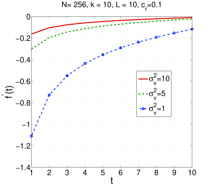
(a) $K=10$

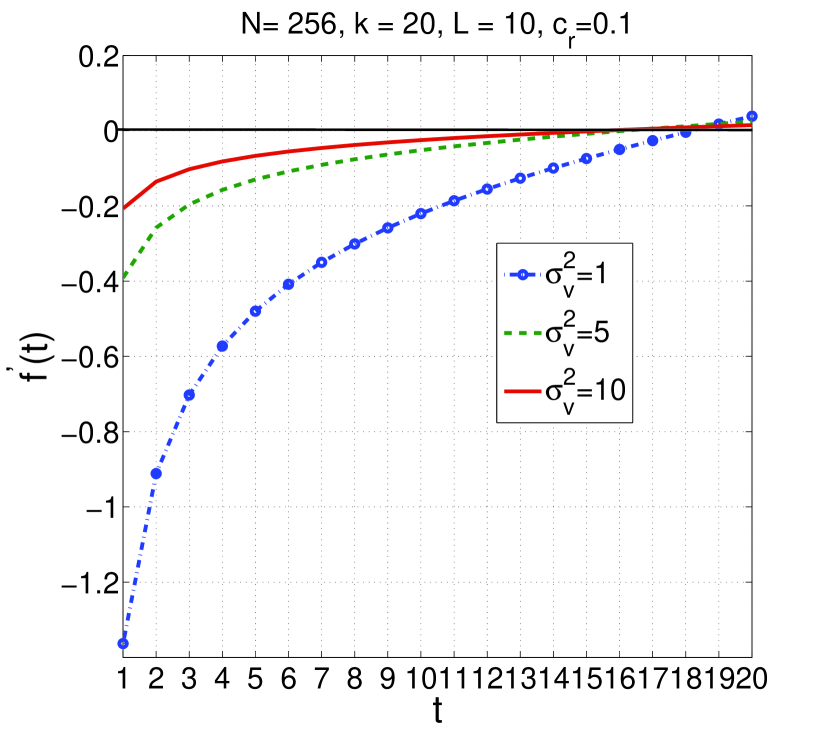
(b) $K=20$

Figure 1: Behavior of $f^{\prime}(t)$ and $P_{d}(t)\approx Q(f(t))$; $N=256$, $L=10$, $c_{r}=0.1$

The above analysis provides insights on sparse signal detection when the minimum size of the partial support set is computed under certain assumptions on the sparse signals. In practice, the desired fraction of the support of the sparse signal needs to be estimated based on the available data when it is not known a priori whether the signal is present or not. In the following section, we consider several extensions of the OMP algorithm to detect the presence of a sparse signal by estimating the partial support of given size in centralized as well as distributed settings.

IV OMP Based Sparse Signal Detection via Partial Support Set Estimation

OMP is a greedy algorithm developed for sparse signal recovery with a single measurement vector (SMV) [49]. In Algorithm 1, we state the standard OMP for sparse support set estimation (the coefficients can be estimated using least squares estimation). It is noted that, the subscripts of the vectors and matrices corresponding to node index are dropped for brevity.

Inputs: $\mathbf{y}$, $\mathbf{B}$, $k$
Output: An estimate for the support set, $\hat{\mathcal{U}}$

1. Initialize $t=1$, $\hat{\mathcal{U}}(0)=\emptyset$, residual vector $\mathbf{r}_{0}=\mathbf{y}$

2. Find the index $\beta(t)$ such that $\beta(t)=\underset{\omega=1,\cdots,N}{\arg~{}\max}~{}{|\langle\mathbf{r}_{t-1},\mathbf{B}({\omega})\rangle|}$

3. Set $\hat{\mathcal{U}}(t)=\hat{\mathcal{U}}(t-1)\cup\{\beta(t)\}$

4. Compute the projection operator $\mathbf{P}(t)=\mathbf{B}(\hat{\mathcal{U}}(t))\left(\mathbf{B}(\hat{\mathcal{U}}(t))^{T}\mathbf{B}(\hat{\mathcal{U}}(t))\right)^{-1}\mathbf{B}(\hat{\mathcal{U}}(t))^{T}$. Update the residual vector: $\mathbf{r}_{t}=(\mathbf{I}-\mathbf{P}(t))\mathbf{y}$ (note: $\mathbf{B}(\hat{\mathcal{U}}(t))$ denotes the submatrix of $\mathbf{B}$ in which columns are taken from $\mathbf{B}$ corresponding to the indices in $\hat{\mathcal{U}}(t)$)

5. Increment $t=t+1$ and go to step 2 if $t\leq k$, otherwise, stop and set $\hat{\mathcal{U}}=\hat{\mathcal{U}}(t-1)$

Algorithm 1 Standard OMP for sparse support set estimation with SMV

The OMP algorithm was extended to the multiple measurement vector case in [25, 39] which is termed simultaneous OMP (S-OMP). First, we consider that all the compressed observations are available at the fusion center. In Algorithm 2, we extend the S-OMP algorithm for sparse signal detection by first estimating a partial support set of size $T_{0}$ based on compressed observations in (2). This is a simple modification of the S-OMP algorithm.

Inputs: $\{\mathbf{y}_{j}\}_{j=1}^{L},\{\mathbf{B}\}_{j=1}^{L}$, $T_{0}$
Outputs: Partial support set estimate $\hat{\mathcal{U}}(T_{0})$, Decision statistic $\Lambda_{cent}$, Detection decision

1. Initialize $t=1$, $\hat{\mathcal{U}}(0)=\emptyset$, residual vector $\mathbf{r}_{j,0}=\mathbf{y}_{j}$ for $j=1,\cdots,L$

2. For $t=1$ to $t=T_{0}$

3. Find the index $\beta(t)$ such that

   $$\beta(t)=\underset{\omega=1,\cdots,N}{\arg~{}\max}~{}\sum_{j=1}^{L}{{|\langle\mathbf{r}_{j,t-1},\mathbf{B}_{j}(\omega)\rangle|}}$$

4. Set $\hat{\mathcal{U}}(t)=\hat{\mathcal{U}}(t-1)\cup\{\beta(t)\}$

5. Compute the orthogonal projection operator: $\mathbf{P}_{j,t}=\mathbf{B}_{j}(\hat{\mathcal{U}}(t))\left(\mathbf{B}_{j}(\hat{\mathcal{U}}(t))^{T}\mathbf{B}_{j}(\hat{\mathcal{U}}(t))\right)^{-1}\mathbf{B}_{j}(\hat{\mathcal{U}}(t))^{T}$           for $j=1,\cdots,L$
   Update the residual: $\mathbf{r}_{j,t}=(\mathbf{I}-\mathbf{P}_{j,t})\mathbf{y}_{j}$ for $j=1,\cdots,L$

6. End For

7. Set $\hat{\mathcal{U}}(T_{0})=\hat{\mathcal{U}}(t)$

8. Detection decision:
   If $\Lambda_{cent}=\sum_{j=1}^{L}||\mathbf{P}_{j,T_{0}}\mathbf{y}_{j}||_{2}^{2}\geq\tau_{0}$, $\mathcal{H}_{1}$ is true, otherwise $\mathcal{H}_{0}$ is true where $\tau_{0}$ is the threshold.

Algorithm 2 S-OMP based sparse signal detection: centralized approach

In a centralized setting, each node has to transmit its length-$M$ compressed measurement vector to the fusion center so that the fusion center processes $\{\mathbf{y}_{l},\cdots,\mathbf{y}_{L}\}$ to make the detection decision. While this reduces the communication burden compared to forwarding uncompressed data vectors of length-$N$, in the following we consider further reduction of information to be transmitted by each node. We propose two distributed algorithms and they differ from each other in terms of the communication overhead.

Inputs: (At the $j$-th node) $\mathbf{y}_{j},\mathbf{B}_{j}$, $T_{0}$ for $j=1,\cdots,L$
Outputs: (At the $j$-th node) Partial support set estimate $\hat{\mathcal{U}}_{j}$, (At the fusion center) Decision statistic $\Lambda_{dist1}$, Detection decision
Initialization:
At the $j$-th node: $\hat{\mathcal{U}}_{j}(0)=\emptyset$, residual vector $\mathbf{r}_{j,0}=\mathbf{y}_{j}$ for $j=1,\cdots,L$.

1. At the $j$-th node for $j=1,\cdots,L$

2. For $t=1$ to $t=T_{0}$

3. Find the index $\beta_{j}(t)$ such that $\beta_{j}(t)=\underset{\omega=1,\cdots,N}{\arg~{}\max}~{}{|\langle\mathbf{r}_{j,t-1},\mathbf{B}_{j}(\omega)\rangle|}$

4. Set $\hat{\mathcal{U}}_{j}(t)=\hat{\mathcal{U}}_{j}(t-1)\cup\{\beta_{j}(t)\}$

5. Compute the projection operator $\mathbf{P}_{j,t}=\mathbf{B}_{j}(\hat{\mathcal{U}}_{j}(t))\left(\mathbf{B}_{j}(\hat{\mathcal{U}}_{j}(t))^{T}\mathbf{B}_{j}(\hat{\mathcal{U}}_{j}(t))\right)^{-1}\mathbf{B}_{j}(\hat{\mathcal{U}}_{j}(t))^{T}$. Update the residual vector: $\mathbf{r}_{j,t}=(\mathbf{I}-\mathbf{P}_{j,t})\mathbf{y}_{j}$

6. End For

7. Set $\hat{\mathcal{U}}_{j}=\hat{\mathcal{U}}_{j}(T_{0})$ and $\mathbf{P}_{j,\hat{\mathcal{U}}_{j}}=\mathbf{P}_{j,T_{0}}$

8. Compute $\Lambda_{j}=||\mathbf{P}_{j,\hat{\mathcal{U}}_{j}}\mathbf{y}_{j}||_{2}^{2}$ and transmit $\Lambda_{j}$ to the fusion center

9. At the fusion center

10. Receive $\Lambda_{j}$ for $j=1,\cdots,L$

11. Compute the decision statistic $\Lambda_{dist1}=\sum_{j=1}^{L}\Lambda_{j}$

12. Detection decision: if $\Lambda_{dist1}\geq\tau_{0}$ decide $\mathcal{H}_{1}$, otherwise decide $\mathcal{H}_{0}$

Algorithm 3 OMP based sparse signal detection: distributed approach 1

A simple version resulting in low communication overhead is to obtain the length $T_{0}$ support set independently at each node and compute a local decision statistic which is then transmitted to the fusion center. The fusion center then combines the local contributions to obtain the final decision statistic. This algorithm is presented in Algorithm 3. Based on the partial support set $\hat{\mathcal{U}}_{j}$ of size $T_{0}$ obtained in step 6, $\Lambda_{j}=||\mathbf{P}_{j,\hat{\mathcal{U}}_{j}}\mathbf{y}_{j}||_{2}^{2}$ is computed and transmitted to the fusion center by the $j$-th node for $j=1,\cdots,L$. Then, the fusion center computes the decision statistic $\Lambda_{dist1}$ as given in step 9 in Algorithm 3. Intuitively, it is expected that Algorithm 2 performs better than Algorithm 3. However, in the following, we show that this is not true always (for certain values of $M$ and $T_{0}$).

IV-A Comparing Algorithms 2 and 3

It is noted that the $j$-th element in the sum in $\Lambda_{cent}$ in Algorithm 2 accounts for the power of the compressed observations projected on to the subspace spanned by the columns of $\mathbf{B}_{j}$ for $j=1,\cdots,L$ indexed by the same set $\hat{\mathcal{U}}(T_{0})$. On the other hand, $j$-th element in the sum in $\Lambda_{dist1}$ in Algorithm 3 represents the power of the compressed observations projected on to the subspace spanned by the columns of $\mathbf{B}_{j}$ indexed by $\hat{\mathcal{U}}_{j}$ which in general can be different for $j=1,\cdots,L$. Thus, when $M$ is not very large, there can be at least one correct index in $\{\mathcal{U}_{j}\}_{j=1}^{L}$ although $\hat{\mathcal{U}}(T_{0})$ does not contain any correct index, especially when $T_{0}$ is also small. In that case, all the elements in the sum in $\Lambda_{cent}$ correspond to the power of the compressed observations projected on to a noise subspace while there can be at least one element in the sum in $\Lambda_{dist1}$ that accounts for the power projected into the signal subspace leading to better detection performance by Algorithm 3. We further analyze this scenario when $T_{0}=1$.

Let $P_{1}$ be the probability that $\beta(1)$ (to avoid confusion while referring to the two algorithms in the following discussion, we denote this as $\beta^{c}(1)$) estimated at step 3 in Algorithm 2 is a correct index under $\mathcal{H}_{1}$. Similarly, let $P_{2}$ be the probability that at least one $\beta_{j}(1)$ (we denote this as $\beta^{d}_{j}(1)$) for $j=1,\cdots,L$ estimated at step 2 in Algorithm 3 is correct under $\mathcal{H}_{1}$. Then we have,

$$P_{1} = Pr(\beta^{c}(1)\in\mathcal{U}|\mathcal{H}_{1})$$

$$= Pr\left(\left\{\underset{\omega=1,\cdots,N}{\arg~{}\max}~{}\sum_{j=1}^{L}{{|\langle\mathbf{y}_{j},\mathbf{B}_{j}(\omega)\rangle|}}\right\}\in\mathcal{U}|\mathcal{H}_{1}\right).$$

On the other hand,

$$P_{2} = Pr(\beta^{d}_{1}(1)\in\mathcal{U}~{}\mathrm{or},\cdots,\mathrm{or}~{}\beta^{d}_{L}(1)\in\mathcal{U}|\mathcal{H}_{1}).$$ (30)

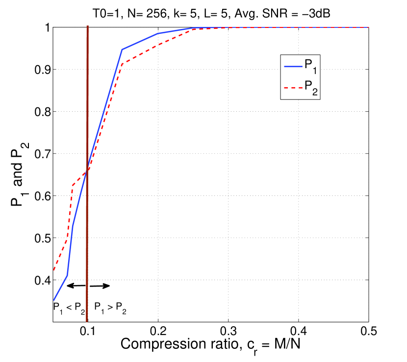
(a) $k=5$, $\mathrm{SNR}=-3dB$

(b) $k=10$, $\mathrm{SNR}=0dB$

Figure 2: Comparison of $P_{1}$ in (34) and $P_{2}$ in (32) as $c_{r}=M/N$ varies

Authors in [49] and [25], respectively, consider the conditions under which OMP (with a single measurement vector) and S-OMP (with multiple measurements vectors) are capable of recovering the complete support set while we focus here only on $T_{0}=1$. Let us partition $\mathbf{B}_{j}$ as $\mathbf{B}_{j}=[\bar{\mathbf{B}}_{j}~{}\tilde{\mathbf{B}}_{j}]$ where $\bar{\mathbf{B}}_{j}$ and $\tilde{\mathbf{B}}_{j}$ are submatrices of $\mathbf{B}_{j}$ with $\bar{\mathbf{B}}_{j}$ containing the columns of $\mathbf{B}_{j}$ indexed by $\mathcal{U}$, while $\tilde{\mathbf{B}}_{j}$ contains the rest of the columns of $\mathbf{B}_{j}$ for $j=1,\cdots,L$. Let

$$\rho_{j}(\mathbf{y}_{j})=\frac{||\tilde{\mathbf{B}}_{j}^{T}\mathbf{y}_{j}||_{\infty}}{||\bar{\mathbf{B}}_{j}^{T}\mathbf{y}_{j}||_{\infty}}$$ (31)

where $||\cdot||_{\infty}$ is the infinity norm of a vector (or a matrix). Then $P_{2}$ in (30) can be expressed as,

$$P_{2} = Pr(\rho_{1}(\mathbf{y}_{1})<1~{}\mathrm{or},\cdots,\mathrm{or}~{}\rho_{L}(\mathbf{y}_{L})<1|\mathcal{H}_{1})$$ (32)

$$= 1-\prod_{j=1}^{L}Pr(\rho_{j}(\mathbf{y}_{j})>1|\mathcal{H}_{1})$$

where the second equality is due to the fact that the multiple nodes estimate the indices independently. In order to compute $P_{1}$, let

$$\rho_{c}(\mathbf{Y})=\frac{||[\tilde{\mathbf{B}}_{1}^{T}\mathbf{y}_{1},\cdots,\tilde{\mathbf{B}}_{L}^{T}\mathbf{y}_{L}]||_{\infty}}{||[\bar{\mathbf{B}}_{1}^{T}\mathbf{y}_{1},\cdots,\bar{\mathbf{B}}_{L}^{T}\mathbf{y}_{L}]||_{\infty}}$$ (33)

where $[\tilde{\mathbf{B}}_{1}^{T}\mathbf{y}_{1},\cdots,\tilde{\mathbf{B}}_{L}^{T}\mathbf{y}_{L}]$ denotes the matrix in which the $j$-th column is $\tilde{\mathbf{B}}_{j}^{T}\mathbf{y}_{j}$ for $j=1,\cdots,L$. Then we have,

$$P_{1}=Pr(\rho_{c}(\mathbf{Y})<1).$$ (34)

It is difficult to find exact analytical expressions for $P_{1}$ and $P_{2}$ in (34) and (32), respectively. Thus, in Fig. 2 we plot $P_{1}$ and $P_{2}$ obtained numerically as the compression ratio $c_{r}=\frac{M}{N}$ varies for different values of $k$ and $L$. It can be observed that there is a threshold for $c_{r}$ for which $P_{1}>P_{2}$. In the region of $c_{r}$ where $P_{2}>P_{1}$, we expect Algorithm 3 to perform better than Algorithm 2 which is observed in the numerical results section. Thus, Algorithm 3 is promising in terms of both performance and the communication overhead when $c_{r}$ (or $M$) is small. However, as $c_{r}$ increases, Algorithm 2 performs better than Algorithm 3. It is more likely that Algorithm 2 estimates all the $T_{0}$ indices correctly compared to the event that all the nodes estimate all the $T_{0}$ indices correctly in Algorithm 3 as $M$ increases.

Inputs: (At the $j$-th node) $\mathbf{y}_{j},\mathbf{B}_{j}$, $T_{0}$ for $j=1,\cdots,L$
Outputs: (At the fusion center) Partial support set estimate $\hat{\mathcal{U}}$, Decision statistic $\Lambda_{dist2}$, Detection decision
Initialization:
At the $j$-th node: $\hat{\mathcal{U}}_{j}(0)=\emptyset$, residual vector $\mathbf{r}_{j,0}=\mathbf{y}_{j}$ for $j=1,\cdots,L$.

1. At the $j$-th node for $j=1,\cdots,L$

2. For $t=1$ to $t=T_{0}$

3. Find the index $\beta_{j}(t)$ such that $\beta_{j}(t)=\underset{\omega=1,\cdots,N}{\arg~{}\max}~{}{|\langle\mathbf{r}_{j,t-1},\mathbf{B}_{j}(\omega)\rangle|}$

4. Set $\hat{\mathcal{U}}_{j}(t)=\hat{\mathcal{U}}_{j}(t-1)\cup\{\beta_{j}(t)\}$

5. Compute the projection operator $\mathbf{P}_{j,t}=\mathbf{B}_{j}(\hat{\mathcal{U}}_{j}(t))\left(\mathbf{B}_{j}(\hat{\mathcal{U}}_{j}(t))^{T}\mathbf{B}_{j}(\hat{\mathcal{U}}_{j}(t))\right)^{-1}\mathbf{B}_{j}(\hat{\mathcal{U}}_{j}(t))^{T}$. Update the residual vector: $\mathbf{r}_{j,t}=(\mathbf{I}-\mathbf{P}_{j,t})\mathbf{y}_{j}$

6. End For

7. Set $\hat{\mathcal{U}}_{j}=\hat{\mathcal{U}}_{j}(T_{0})$ and transmit $\mathcal{U}_{j}$ to the fusion center

8. Receive $\hat{\mathcal{U}}$ from the fusion center

9. Compute $\Lambda_{j}=||\mathbf{P}_{j,\hat{\mathcal{U}}}\mathbf{y}_{j}||_{2}^{2}$ and transmit $\Lambda_{j}$ to the fusion center

10. At the fusion center

11. Receive $\hat{\mathcal{U}}_{j}$ for $j=1,\cdots,L$

12. Compute $\hat{\mathcal{U}}=f(\{\hat{\mathcal{U}}_{j}\}_{j=1}^{L})$ as discussed in subsection IV-B and transmit to all the nodes

13. Receive $\Lambda_{j}$ for $j=1,\cdots,L$ from the nodes

14. Compute the decision statistic $\Lambda_{dist2}=\sum_{j=1}^{L}\Lambda_{j}$

15. Detection decision: if $\Lambda_{dist2}\geq\tau_{0}$ decide $\mathcal{H}_{1}$, otherwise decide $\mathcal{H}_{0}$

Algorithm 4 OMP based sparse signal detection: distributed approach 2

IV-B Description of Algorithm 4

When estimating the partial support of size $T_{0}$ at each node, Algorithm 3 does not account for the fact that all the nodes have the same support in the support set estimation stage. In the second distributed algorithm presented in Algorithm 4, the fact that all the nodes share the same support is taken into account by fusion as described below. In Algorithm 4, each node estimates a partial support set of size $T_{0}$ after running $T_{0}$ iterations of the standard OMP algorithm independently. Then, the $T_{0}$-length support set, denoted by $\hat{\mathcal{U}}_{j}$ is transmitted by the $j$-th node to the fusion center. Based on $\{\hat{\mathcal{U}}_{j}\}_{j=1}^{L}$, the fusion center estimates a length-$k$ support set $\hat{\mathcal{U}}$ and transmits it back to the nodes. The $j$-th node then computes $\Lambda_{j}=||\mathbf{P}_{j,\hat{\mathcal{U}}}\mathbf{y}_{j}||_{2}^{2}$ where $\mathbf{P}_{j,\hat{\mathcal{U}}}=\mathbf{B}_{j}(\hat{\mathcal{U}})\left(\mathbf{B}_{j}(\hat{\mathcal{U}})^{T}\mathbf{B}_{j}(\hat{\mathcal{U}})\right)^{-1}\mathbf{B}_{j}(\hat{\mathcal{U}})^{T}$ and transmits back to the fusion center. The fusion center computes the decision statistic $\Lambda_{dist2}=\sum_{j=1}^{L}\Lambda_{j}$.

In this algorithm, each node communicates with the fusion center twice (steps 6 and 8). The communication overhead in step 8 is similar to that in Algorithm 3. In step 6, the estimated partial support set $\mathcal{U}_{j}$ of size $T_{0}$ is transmitted to the fusion center. Then, the fusion center computes an updated estimate for the support set which can be larger than $T_{0}$ and of course less than $k$. Let $I$ be the set containing all the indices (can have multiple occurrences of the same index) in $\{\hat{\mathcal{U}}_{j}\}_{j=1}^{L}$. Let $D$ be a set which contains all the distinct values in $I$ ordered in a descending manner based on the frequency of occurrence in $I$. Let $\mathrm{length}(D)$ denote the number of elements in $D$. If each node estimates $T_{0}$ correct locations of the support via OMP, $\mathrm{length}(D)$ can have maximum value of $k$. However, if there is an error in estimating the support after $T_{0}$ iterations at a given node, $\mathrm{length}(D)$ can be greater than $k$; in the worst case, $\mathrm{length}(D)=T_{0}L$. Thus, we have, $T_{0}\leq\mathrm{length}(D)\leq T_{0}L$. We compute $\hat{\mathcal{U}}$ as $\hat{\mathcal{U}}=D(1:\min(\mathrm{length}(D),k))$. Thus, in this algorithm, partial support estimates are fused (via the majority rule) at the fusion center to compute an enlarged (or sometimes complete) support set.

When comparing Algorithms 3 and 4, the additional communication overhead required by each node in Algorithm 4 comes from the need for transmitting indices of length $T_{0}$ in step 6. Thus, the communication overhead in Algorithm 4 can be reduced by letting all the nodes to run only $1$ iteration of the OMP algorithm; i.e., $T_{0}=1$. As illustrated in the numerical results section, Algorithm 4 provides promising performance when $T_{0}=1$ since the local decision statistic is computed based on a fused and enlarged support set compared to both Algorithms 3 and 2. However, as $T_{0}$ increases, it can be observed that Algorithm 3 performs better than Algorithm 4 even though the communication overhead of Algorithm 4 increases as $T_{0}$ increases. Thus, the improved performance of Algorithm 4 is significant with only small $T_{0}$ which is desirable. Further, under certain conditions, both distributed algorithms perform better than the centralized version presented in Algorithm 2. More details are provided in the numerical results section.

IV-C Communication complexity

In this subsection, we summarize the communication complexities of Algorithms 2-4 in terms of the number of messages to be transmitted by each node to the fusion center.

• Algorithm 2: $M$ messages per node

• Algorithm 3: $1$ message per node

• Algorithm 4: $T_{0}+1$ messages per node; needs feedback from the fusion center.

V Numerical Results

In this section, we illustrate the performance of sparse signal detection based on the knowledge of a partial support set. The signals are assumed to be sparse in the canonical basis, so that $\mathbf{B}_{j}=\mathbf{A}_{j}$ for $j=1,\cdots,L$. The elements of $\mathbf{A}_{j}$ are drawn from a standard normal ensemble and then $\mathbf{A}_{j}$ is orthogonalized so that $\mathbf{A}_{j}\mathbf{A}_{j}^{T}=\mathbf{I}$. The sparse support set is selected from $[1,N]$ uniformly. The coefficients of $\mathbf{s}_{j}$ for $j=1,\cdots,L$ are taken uniformly from $[-b,-a]\bigcup[a,b]$. For given $a$ and $b$, the SNR is varied by changing $\sigma_{v}^{2}$. The average (over all the nodes) uncompressed SNR, $\bar{\gamma}$, is defined as $\bar{\gamma}=\sum_{j=1}^{L}\frac{||\mathbf{s}_{j}||_{2}^{2}}{LN\sigma_{v}^{2}}=\sum_{j=1}^{L}\frac{\gamma_{j}}{LN}$ where $\gamma_{j}=\frac{||\mathbf{s}_{j}||_{2}^{2}}{\sigma_{v}^{2}}$. In the following figures, by average SNR, we mean the uncompressed SNR, $\bar{\gamma}$. As defined before, $c_{r}=\frac{M}{N}$ is the compression ratio at a given node. Further, we define $t_{f}=\frac{\hat{t}}{k}$ to be the minimum fraction of the support that needs to be known. First, we illustrate the minimum fraction of support to be known to achieve a desired detection performance level.

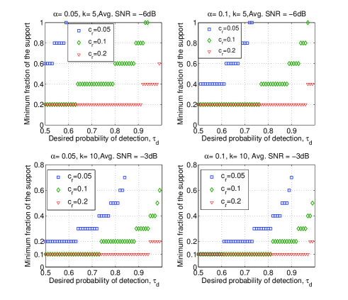
Figure 3: Minimum fraction of the support to be known, $t_{f}$, to achieve a desired detection performance, $N=256$, $L=5$, $\sigma_{v}^{2}=1$

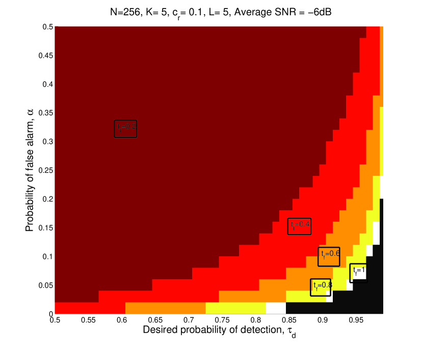
(a) $L=5$, $\mathrm{SNR}=-6dB$, $\sigma_{v}^{2}=1$

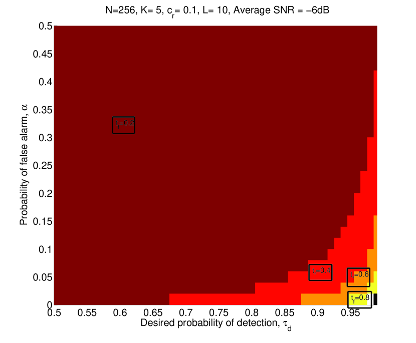
(b) $L=10$, $\mathrm{SNR}=-6dB$, $\sigma_{v}^{2}=1$

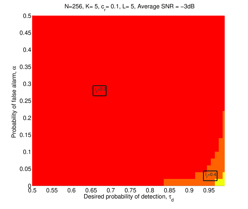
(c) $L=5$, $\mathrm{SNR}=-3dB$, $\sigma_{v}^{2}=0.5$

Figure 4: Minimum fraction of the support to be known, $t_{f}$, to achieve a desired detection performance as $\tau_{d}$ and $\alpha$ vary, values of $\tau_{d}$ and $\alpha$ in the black region cannot be achieved even if all the indices of the support are known correctly; $N=256$, $k=5$, $c_{r}=0.1$

V-A The minimum fraction of the support set to achieve a desired performance level

In Figs. 3 and 4, the minimum fraction of the support set is shown as different parameters vary. We let $a=3$ and $b=4$. In Fig. 3, $t_{f}$ is shown as $\tau_{d}$ varies for different values of $c_{r}$, $\alpha$ and $k$ while keeping $N=256$, $L=5$ and $\sigma_{v}^{2}=1$. It is worth mentioning that the average SNR in the bottom two subplots in Fig. 3 is different from the two top subplots due to the change of $k$ (albeit $\sigma_{v}^{2}$ is kept constant). When $c_{r}$ increases, the fraction of the support set to be estimated becomes small to achieve the desired performance level. For example, in the top left figure, to achieve $\tau_{d}\approx 0.9$, the knowledge of only one index of the support set is sufficient when $c_{r}=0.2$ while it requires the knowledge of $4$ (out of 5) indices when $c_{r}=0.1$. As $c_{r}$ increases, the SNR of the compressed signal increases (although the uncompressed SNR remains the same) resulting in better performance. Similarly, the impact of $\alpha$ and $k$ (thus the uncompressed SNR) on $t_{f}$ is depicted in Fig. 3.

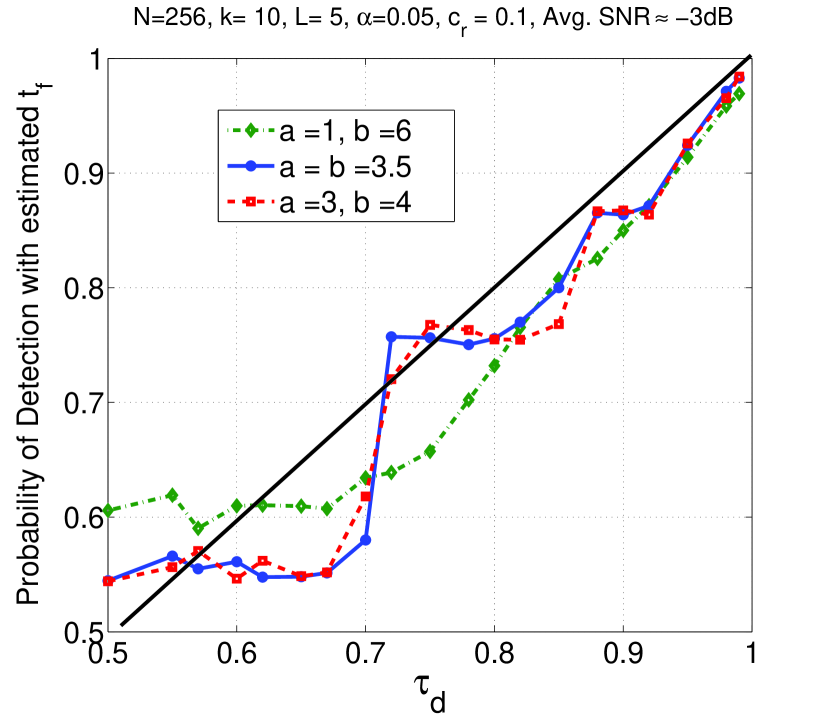
(a) $N=256$, $k=10$, $\sigma_{v}^{2}=1$, $\alpha=0.05$, $c_{r}=0.1$

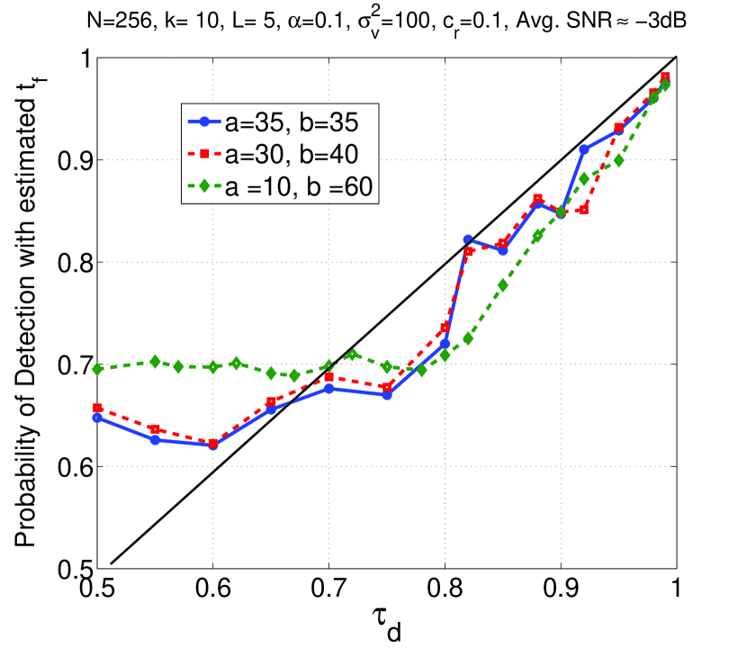
(b) $N=256$, $k=10$, $\sigma_{v}^{2}=100$, $\alpha=0.1$, $c_{r}=0.1$

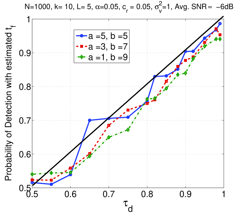
(c) $N=1000$, $k=10$, $\sigma_{v}^{2}=1$, $\alpha=0.05$, $c_{r}=0.05$

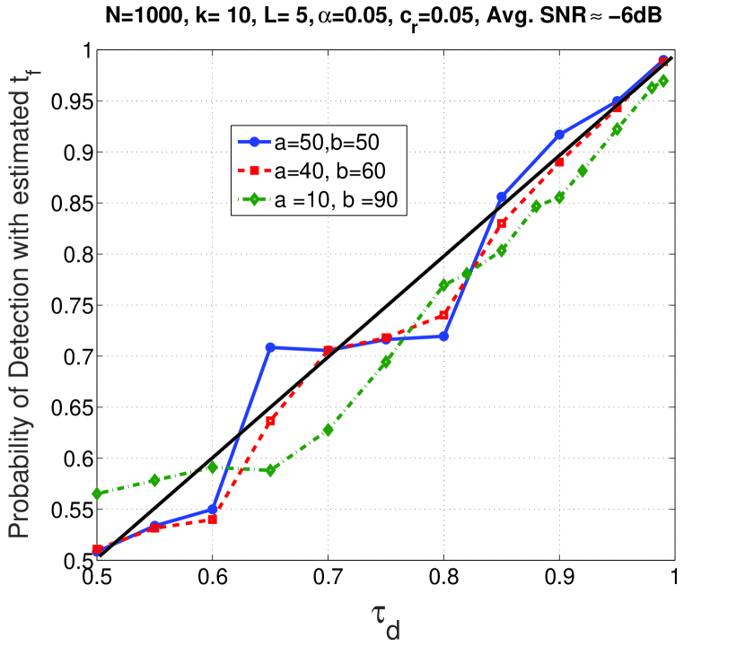
(d) $N=1000$, $k=10$, $\sigma_{v}^{2}=100$, $\alpha=0.05$, $c_{r}=0.05$

Figure 5: Impact of nonzero coefficients

In resource constrained sensor networks working in a distributed setting, it is desirable to keep $c_{r}$ as small as possible. In Fig. 4, the impact of $L$ and uncompressed SNR on $t_{f}$ is illustrated when $c_{r}$ is kept at a lower value ($c_{r}=0.1$) for $k=5$ and $N=256$. The regions of $\tau_{d}$ and $\alpha$ that can be achieved with a specific $t_{f}$ obtained from Proposition 1 are shown in different colors. The black portion corresponds to the regions of $\tau_{d}$ and $\alpha$ that cannot be achieved even if all the support indices corresponding to nonzero coefficients of sparse signals are known. It can be seen that, when $c_{r}$ is small, the desired detection performance can be achieved by estimating only a very small fraction of the support set when either $\bar{\gamma}$ is large or by increasing $L$. For example, as depicted in Fig. 4 (c) when $L=5$ and uncompressed $\mathrm{SNR}=-3dB$, almost all the regions of $\tau_{d}$ and $\alpha$ can be achieved by knowing only one or two indices of the support set correctly (so that $t_{f}=0.2$ or $t_{f}=0.4$). In summary, Figures 3 and 4 demonstrate the regions of $k$, $L$, $\bar{\gamma}$, $\tau_{d}$, $\alpha$ and $c_{r}$ so that estimation of only a small fraction of the support is sufficient for sparse signal detection with desired performance.

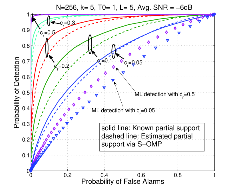
(a) $T_{0}=1$

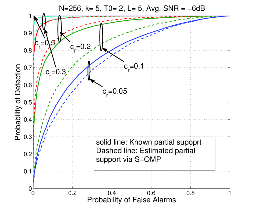
(b) $T_{0}=2$

Figure 6: ROC curves for detection based on partial support set estimation, $k=5$, $N=256$, $L=5$

V-B Impact of the values of nonzero coefficients

The minimum fraction of nodes in Proposition 1 was computed under the assumption that the nonzero coefficients of the sparse signals do not deviate much from each other. In this subsection, we analyze the results in Proposition 1 when this assumption is relaxed. In Fig. 5, we plot the performance of the detector (5) when the size of the support is computed based on Proposition 1 given that the nonzero coefficients are actually far from each other. For a given $\tau_{d}$ on the x-axis, $t_{f}$ is computed as in (25). Substituting $T_{0}=t_{f}k$ in (5), the probability of detection (obtained numerically) with the decision statistic (5) is shown on the y-axis. It is noted that since Proposition 1 does not give a clue on which $T_{0}$ indices should be selected, we get $T_{0}$ indices uniformly from $\mathcal{U}$. The first two subplots correspond to a small problem size while last two subplots consider relatively large $N$. For both problem sizes, relatively large and small values for $a$ and $b$ are considered. It is noted that $a$, $b$ and $\sigma_{v}^{2}$ are changed accordingly so that the average SNR remains approximately the same for given $N$ and $L$. The desired scenario is that the curves stay close or above the black (y=x) line. It can be seen that when $N$ is large, all the curves remain fairly close to (or above) the black line for most values of $\tau_{d}$. When $N$ is not very large (subplots (a) and (b)), performance degradation can be seen for some values of $\tau_{d}$. However, for relatively large values of $\tau_{d}$ (which is the most interesting scenario), there is no significant performance degradation using Proposition 1 even the coefficient values deviate quite significantly from each other irrespective of the problem size.

V-C Performance of sparse signal detection in a centralized setting: Detection with known partial support and via S-OMP

In this subsection, we compare the detection performance when the partial support set is exactly known and it is estimated via S-OMP in a centralized setting. In Fig. 6, we show receiver operating characteristic (ROC) curves with $10^{4}$ Monte carlo runs. In the case where the partial support set is known, $T_{0}$ indices are selected randomly from $\mathcal{U}$ and the results are averaged over $20$ trials. In the S-OMP based detection, $T_{0}$ indices are selected according to Algorithm 2. In Fig. 6 (a), $T_{0}=1$ while in Fig. 6 (b), $T_{0}=2$. The other parameters $k$, $L$, and $N$ remain the same in both subfigures as stated while $a=3$ and $b=4$. In Fig. 6 (a), we further plot the detection performance when the sparse signal is estimated via maximum likelihood (ML) estimation ignoring sparsity; i.e. when the decision statistic is $\Lambda_{ML}=\sum_{j=1}^{L}||\mathbf{P}_{j}\mathbf{y}_{j}||_{2}^{2}$ with $\mathbf{P}_{j}=\mathbf{B}_{j}\left(\mathbf{B}_{j}^{T}\mathbf{B}_{j}\right)^{-1}\mathbf{B}_{j}^{T}$. It is observed that exploitation of sparsity even with $T_{0}=1$ outperforms the ML based detection approach and we avoid plotting curves for this comparison in subsequent figures.

It is observed that, for both $T_{0}=1$ and $T_{0}=2$, the performance of the S-OMP based detection is close to the performance with known partial support for very small and relatively large $c_{r}$ values. When $c_{r}$ is very small (e.g $\approx 0.05$ in Fig.6), the SNR of the compressed observation vector is small, thus even with the known support set, the power of the compressed observations projected onto the known subspace is not significant compared to the analogous noise power. Thus, close (and poor) performance is observed when the partial support is known or estimated. On the other hand, when $c_{r}$ is large, the estimated support set of size $T_{0}$ via Algorithm 2 is more accurate, resulting in close performance to the case where the partial support is exactly known. However, when $c_{r}$ is moderate (i.e. $\approx.1$ or $.2$ in Fig. 6)), S-OMP based detection has a performance gap compared to detection with known partial support of the same size. When $c_{r}$ takes such values, the accuracy of the estimated partial support set via S-OMP is not quite good thus, resulting in a performance gap. In such regions of $c_{r}$ where compressed measurements per node are not sufficient to provide a good estimate of the support set via S-OMP, the detection performance is improved with the two distributed algorithms as will be illustrated next.

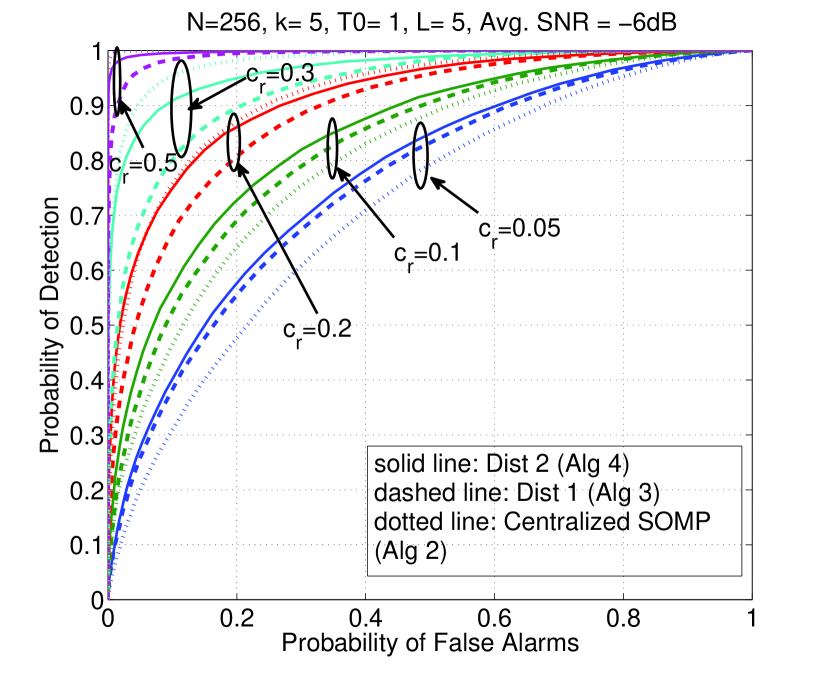
(a) $N=256$, $k=5$, Average $\mathrm{SNR}=-6dB$

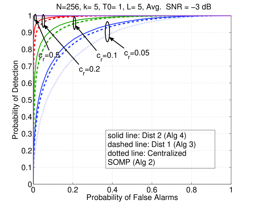
(b) $N=256$, $k=5$, Average $\mathrm{SNR}=-3dB$

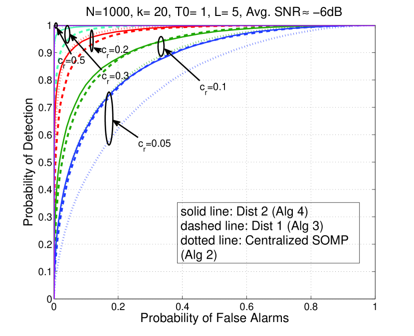
(c) $N=1000$, $k=20$, $T_{0}=1$

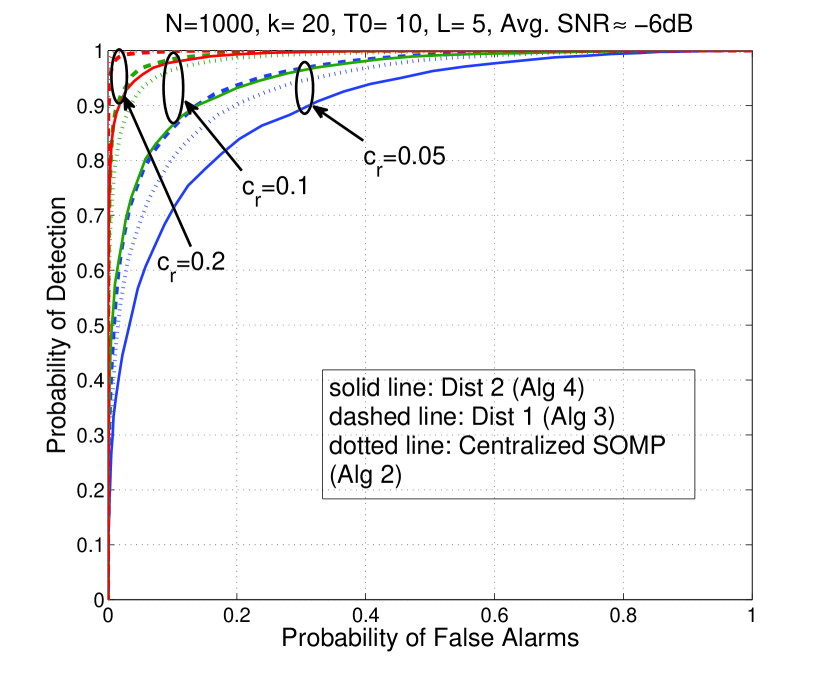
(d) $N=1000$, $k=20$, $T_{0}=10$

Figure 7: ROC curves for OMP based detection; S-OMP and two distributed approaches

V-D Performance comparison of S-OMP based and two distributed OMP based algorithms

In Fig. 7, ROC curves are plotted for different values of $c_{r}$ for centralized and two distributed OMP based algorithms. We let $a=3$ and $b=4$. In Figs. 7 (a) and (b), we consider relatively a small sized problem with $N=256$, $k=5$, $L=5$, $T_{0}=1$ and the average SNR (uncompressed) is varied by changing $\sigma_{v}^{2}$. On the other hand, in Figs. 7 (c) and (d), a bigger sized problem is considered so that $N=1000$, $k=20$, $L=5$, the average SNR (uncompressed) $=-6~{}dB$ and $T_{0}$ is varied. We make several important observations here.

1. When $c_{r}$ and $T_{0}$ are quite small, the S-OMP based algorithm performs worse than the two distributed algorithms (subplots (a), (b) and (c)). This (counter-intuitive) phenomenon was discussed in detail in Subsection IV-A for $T_{0}=1$ considering Algorithms 2 and 3. Thus, Algorithm 3 produces a better decision statistic to discriminate between the noise and the signal. Similar explanation holds for Algorithm 4 which provides even better results compared to Algorithm 3 due to the fusion of support indices estimated at multiple nodes. Thus, when $M$ (thus $c_{r}$) is not sufficient to provide accurate estimates for the support set after $T_{0}$ iterations via S-OMP, the two distributed algorithms, by fusion, provide better performance.

2. When $T_{0}$ is relatively large, from Fig. 7 (d), it is seen that Algorithm 4 works relatively poorly compared to the other two algorithms. As discussed in Section IV-B and seen in Fig. 7 (a), (b) and (c), Algorithm 4 is promising in terms of communication complexity only when $T_{0}$ is small.

It is noted that, in the S-OMP algorithm, raw compressed observations are fused in computing the support set indices and the decision statistic for detection is obtained based on such estimated indices. On the other hand, in Algorithms 3 and 4, individually computed local decision statistics are fused to compute the final decision statistic at the fusion center. From Fig. 7, it is seen that, measurement fusion via S-OMP provides better performance only when $c_{r}$ is relatively large. This is an important observation which is somewhat counter intuitive, since one would expect a centralized scheme to work better than any distributed approach. There are several reasons. One is that S-OMP is not an optimal method of computing the sparse support set although it provides promising results when $c_{r}$ exceeds a certain threshold. When $c_{r}$ is small, there can be other variants (such as two distributed algorithms presented here) of OMP other than S-OMP that would provide better performance in sparse support recovery. Another reason is that, we focus on partial signal recovery (and detection based on that) but not on complete signal recovery. Thus, we conclude that better decision statistics for detection based on OMP can be computed in a distributed setting compared to a centralized setting under certain conditions.

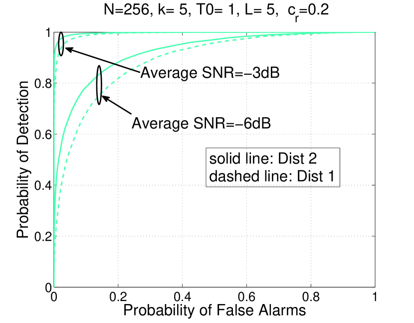
(a) $T_{0}=1$, $L=5$

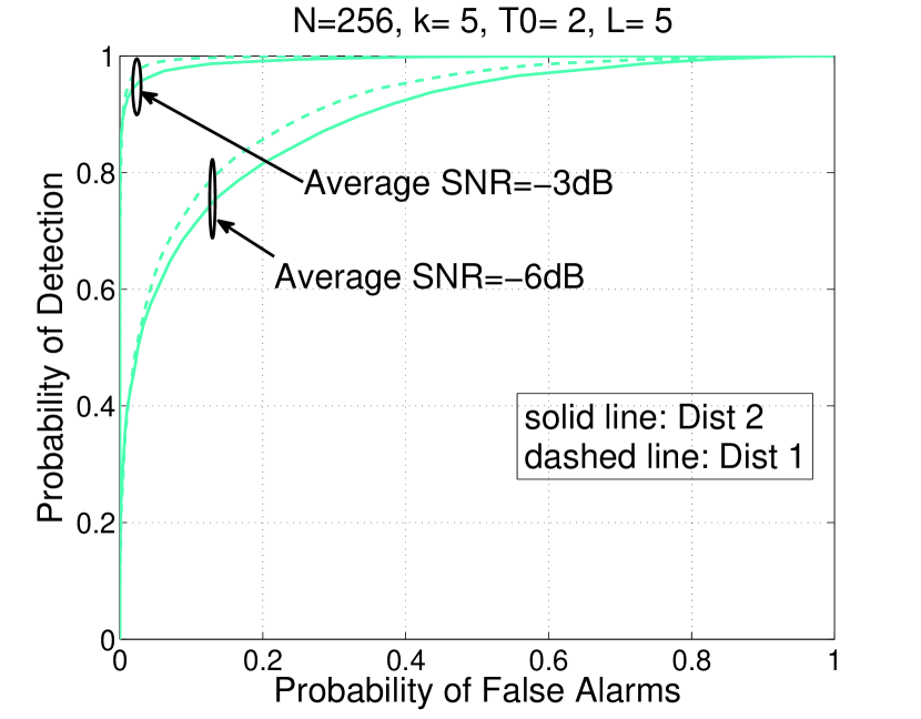
(b) $T_{0}=2$, $L=5$

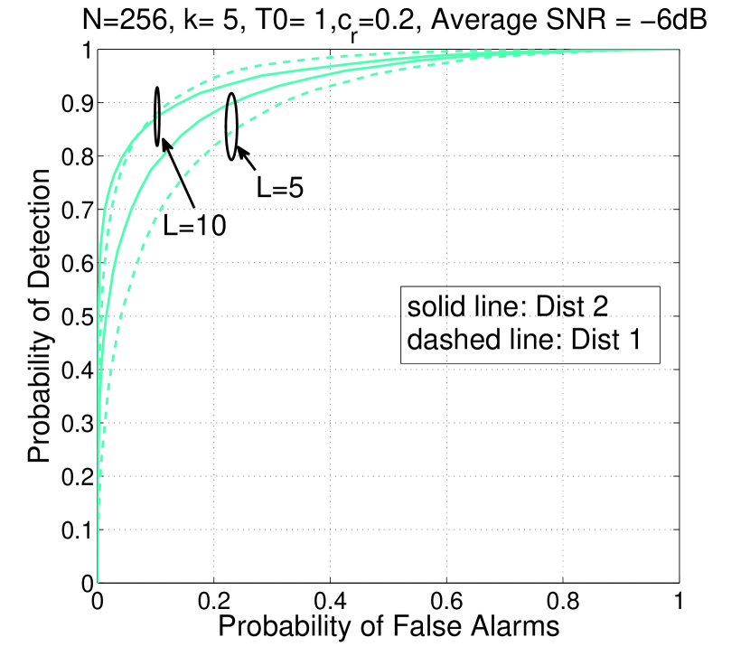
(c) $T_{0}=1$, $\mathrm{SNR}=-6dB$

Figure 8: Performance comparison of two distributed algorithms, $k=5$, $N=256$, $c_{r}=0.2$

V-E Performance comparison of two distributed OMP based algorithms

The first distributed algorithm presented in Algorithm 3 requires small communication overhead compared to the second distributed algorithm in Algorithm 4. In Fig. 8, we compare the performance of the two distributed algorithms as $T_{0}$, SNR values and $L$ vary. When $T_{0}=1$, it can be seen that Algorithm 4 performs better than Algorithm 3 for both SNR values considered when $L=5$. However, as seen in Fig. 8(b), when $T_{0}$ is increased, Algorithm 3 performs better than Algorithm 4. The additional communication overhead required by Algorithm 4 is not worth it as $T_{0}$ increases compared to Algorithm 3. Thus, it is seen that the Algorithm 4 is promising and worth the additional communication overhead needed only when $T_{0}=1$ and $L$ is relatively small, which are the most desirable scenarios.

VI Conclusion

In this paper, we discussed the use of a CS measurement scheme for sparse signal detection when multiple sparse signals observed by distributed nodes share the same sparsity pattern. We showed that by estimating only a fraction of the support with less computational power than that is required for complete signal recovery, a reliable decision statistic can be designed. First, we analyzed the minimum fraction of the support set to be estimated to achieve a desired detection performance in a centralized setting. Then, OMP based algorithms were developed to jointly estimate a partial support set and perform detection in centralized as well as distributed settings. It was shown that with each node estimating only one index of the support set, a reliable detection decision can be made by appropriate fusion among nodes. Further, when the number of compressed measurements acquired at each node is small, the two distributed algorithms (with less communication overhead) are shown to outperform the centralized algorithm (with higher communication overhead). In future work, we will show the efficiency and effectiveness of the proposed algorithms with different real world application scenarios (using real experimental data).

References

- [1] M. Davenport, M. Duarte, Y. Eldar, and G. Kutyniok, Introduction to compressed sensing; Chapter in Compressed Sensing: Theory and Applications. Cambridge University Press, 2012.
- [2] E. Cands, J. Romberg, and T. Tao, “Robust uncertainty principles: exact signal reconstruction from highly incomplete frequency information,” IEEE Trans. Inf. Theory, vol. 52, no. 2, pp. 489 – 509, Feb. 2006.
- [3] E. Cands and T. Tao, “Near-optimal signal recovery from random projections: Universal encoding strategies?” IEEE Trans. Inf. Theory, vol. 52, no. 12, pp. 5406 – 5425, Dec. 2006.
- [4] D. Donoho, “Compressed sensing,” IEEE Trans. Inf. Theory, vol. 52, no. 4, pp. 1289–1306, Apr. 2006.
- [5] E. J. Candès and Y. Plan, “A probabilistic and RIPless theory of compressed sensing,” IEEE Trans. Inf. Theory, vol. 57, no. 11, pp. 7235–7254, 2011.
- [6] Y. C. Eldar and G. Kutyniok, Compressed Sensing: Theory and Applications. Cambridge University Press, 2012.
- [7] R. G. Baraniuk, V. Cevher, M. Duarte, and C.Hegde, “Model based compressed sensing,” IEEE Trans. Inf. Theory, vol. 56, no. 4, pp. 1982–2001, Apr. 2010.
- [8] M. F. Duarte, M. A. Davenport, M. B. Wakin, and R. G. Baraniuk, “Sparse signal detection from incoherent projections,” in Proc. Acoust., Speech, Signal Processing (ICASSP), May 2006.
- [9] J. Haupt and R. Nowak, “Compressive sampling for signal detection,” in Proc. Acoust., Speech, Signal Processing (ICASSP), vol. 3, Honolulu, Hawaii, Apr. 2007, pp. III–1509 – III–1512.
- [10] Z. Wang, G. Arce, and B. Sadler, “Subspace compressive detection for sparse signals,” in Proc. Acoust., Speech, Signal Processing (ICASSP), Mar. 2008, pp. 3873–3876.
- [11] J. Meng, H. Li, and Z. Han, “Sparse event detection in wireless sensor networks using compressive sensing,” in 43rd Annual Conf. on Information Sciences and Systems (CISS), Baltimore, MD, Mar. 2009, pp. 181 – 185.
- [12] M. A. Davenport, P. T. Boufounos, M. B. Wakin, and R. Baraniuk, “Signal processing with compressive measurements,” IEEE J. Sel. Topics Signal Process., vol. 4, no. 2, pp. 445 – 460, Apr. 2010.
- [13] T. Wimalajeewa, H. Chen, and P. K. Varshney, “Performance analysis of stochastic signal detection with compressive measurements,” in Annual Asilomar Conf. on Signals, Systems and Computers, Nov. 2010, pp. 913–817.
- [14] R. Zahedi, A. Pezeshki, and E. K. Chong, “Measurement design for detecting sparse signals,” Physical Communication, Compressive Sensing in Communications, vol. 5, no. 2, pp. 64–75, 2012.
- [15] T. Wimalajeewa and P. K. Varshney, “Cooperative sparsity pattern recovery in distributed networks via distributed-OMP,” in Proc. Acoust., Speech, Signal Processing (ICASSP), Vancouver, BC, May 2013, pp. 5288–5292.
- [16] G. Li, H. Zhang, T. Wimalajeewa, and P. K. Varshney, “On the detection of sparse signals with sensor networks based on Subspace Pursuit,” in IEEE Global Conference on Signal and Information Processing (GlobalSIP), Atlanta, GA, Dec. 2014, pp. 438–442.
- [17] B. Kailkhura, T. Wimalajeewa, L. Shen, and P. K. Varshney, “Distributed compressive detection with perfect secrecy,” in 2nd Int. Workshop on Compressive Sensing in Cyber-Physical Systems (CSCPS’14), Oct. 2014.
- [18] B. Kailkhura, T. Wimalajeewa, and P. K. Varshney, “On physical layer secrecy of collaborative compressive detection,” in Annual Asilomar Conf. on Signals, Systems and Computers, 2014.
- [19] H. Zheng, S. Xiao, and X. Wang, “Sequential compressive target detection in wireless sensor networks,” in IEEE Int. Conf. on Communications (ICC), Kyoto,, June 2011, pp. 1 –5.
- [20] B. S. M. R. Rao, S. Chatterjee, and B. Ottersten, “Detection of sparse random signals using compressive measurements,” in Proc. Acoust., Speech, Signal Processing (ICASSP), 2012, pp. 3257–3260.
- [21] J. Cao and Z. Lin, “Bayesian signal detection with compressed measurements,” Information Sciences, pp. 241–253, 2014.
- [22] B. Kailkhura, S. Liu, T. Wimalajeewa, and P. K. Varshney, “Measurement matrix design for compressed detection with secrecy guarantees,” IEEE Wireless Commun. Lett., 2016, Accepted.
- [23] B. Kailkhura, T. Wimalajeewa, and P. K. Varshney, “Collaborative compressive detection with physical layer secrecy constraints,” IEEE Trans. Signal Process., 2016, Submitted.
- [24] G. Reeves and M. Gastpar, “Sampling bounds for sparse support recovery in the presence of noise,” in IEEE Int. Symp. on Information Theory (ISIT), Toronto, ON, Jul. 2008, pp. 2187–2191.
- [25] J. Tropp, A. Gilbert, and M. Strauss, “Algorithms for simultaneous sparse approximation. part I: Greedy pursuit,” Signal Processing, special issue on Sparse approximations in signal and image processing, vol. 86, no. 4, pp. 572–588, 2006.
- [26] ——, “Algorithms for simultaneous sparse approximation. part II: Convex relaxation,” Signal Processing, special issue on Sparse approximations in signal and image processing, vol. 86, no. 4, pp. 589–602, 2006.
- [27] S. F. Cotter, B. D. Rao, K. Engan, and K. Kreutz-Delgado, “Sparse solutions to linear inverse problems with multiple measurement vectors,” IEEE Trans. Signal Process., vol. 53, no. 7, pp. 2477–2488, July 2005.
- [28] J. Chen and X. Huo, “Theoretical results on sparse representations of multiple-measurement vectors,” IEEE Trans. Signal Process., vol. 54, no. 12, pp. 4634–4643, Dec. 2006.
- [29] G. Obozinski, M.Wainwright, and M. Jordan, “Support union recovery in high-dimensional multivariate regression,” Ann. Stat., vol. 39, no. 1, pp. 1–47, 2011.
- [30] D. Wipf and B. Rao, “An empirical bayesian strategy for solving the simultaneous sparse approximation problem,” IEEE Trans. Signal Process., vol. 55, no. 7, pp. 3704–3716, July 2007.
- [31] Y. C. Eldar and H. Rauhut, “Average case analysis of multichannel sparse recovery using convex relaxation,” IEEE Trans. Inf. Theory, vol. 56, no. 1, pp. 505–519, Jan. 2010.
- [32] Y. C. Eldar and M. Mishali, “Robust recovery of signals from a structured union of subspaces,” IEEE Trans. Inf. Theory, vol. 55, no. 11, pp. 5302–5316, Nov. 2009.
- [33] Q. Ling and Z. Tian, “Decentralized support detection of multiple measurement vectors with joint sparsity,” in Proc. Acoust., Speech, Signal Processing (ICASSP), 2011, pp. 2996–2999.
- [34] F. Zeng, C. Li, and Z. Tian, “Distributed compressive spectrum sensing in cooperative multihop cognitive networks,” IEEE J. Sel. Topics Signal Process., vol. 5, no. 1, pp. 37–48, Feb. 2011.
- [35] J. A. Bazerque and G. B. Giannakis, “Distributed spectrum sensing for cognitive radio networks by exploiting sparsity,” IEEE Trans. Signal Process., vol. 58, no. 3, pp. 1847–1862, Mar. 2010.
- [36] Q. Ling and Z. Tian, “Decentralized sparse signal recovery for compressive sleeping wireless sensor networks,” IEEE Trans. Signal Process., vol. 58, no. 7, pp. 3816–3827, July 2010.
- [37] M. Rabbat, J. D. Haupt, A. Singh, and R. D. Nowak, “Decentralized compression and predistribution via randomized gossiping,” in Int. Workshop on Info. Proc. in Sensor Networks (IPSN), Nashville, TN, Apr. 2006.
- [38] S. Patterson, Y. C. Eldar, and I. Keidar, “Distributed sparse signal recovery for sensor networks,” in Proc. Acoust., Speech, Signal Processing (ICASSP), Vancouver, Canada, May 2013.
- [39] D. Baron, M. Duarte, S. Sarvotham, M. B. Wakin, and R. G. Baraniuk, “Distributed compressed sensing,” Rice Univ. Dept. Elect. Comput. Eng. Houston, TX, Tech. Rep. TREE–0612, Nov 2006.
- [40] M. E. Lopes, “Estimating unknown sparsity in compressed sensing,” in 30 Int. Conf. om Machine Learning (JMLR: W CP), Atlanta, GA, 2013, pp. 217–225.
- [41] V. Bioglio, T. Bianchi, and E. Magli, “On the fly estimation of the sparsity degree in compressed sensing using sparse sensing matrices,” in IEEE Int. Conf. on Acoustics, Speech and Signal Processing (ICASSP), South Brisbane, QLD, 2015, pp. 3801–3805.
- [42] L. L. Scharf and B. Friedlander, “Matched subspace detectors,” IEEE Tran. Signal Process., vol. 42, no. 8, pp. 2146 – 2157, Aug. 1994.
- [43] L. T. McWhorter and L. L. Scharf, “Matched subspace detectors for stochastic signals,” in 11th Ann. Workshop on Adaptive Sensor Array Process. (ASAP), Lexington, MA, Mar. 2003.
- [44] Y. Jin and B. Friedlander, “A CFAR adaptive subspace detector for second-order gaussian signal,” IEEE Tran. Signal Process., vol. 53, no. 3, pp. 871 – 884, Mar. 2005.
- [45] H. V. Poor, An Introduction to Signal Detection and Estimation. New York: Springer-Verlag, 1994.
- [46] M. Sankaran, “Approximations to the non-central chi-square distribution,” Biometrika, vol. 50, no. 1-2, pp. 199–204, Dec. 1963.
- [47] M. Junger, T. M. Liebling, D. Naddef, G. L. Nemhausera, W. R. Pulleyblank, G. Reinelt, G. Rinaldi, and L. A. Wolsey, 50 Years of Integer Programming 1958-2008. Springer-Verlag Berlin Heidelber, 2010.
- [48] S. Leyffer, “Deterministic methods for mixed integer nonlinear programming,” Ph.D. dissertation. University of Dundee. Scotland, U.K., 1993.
- [49] J. Tropp and A. Gilbert, “Signal recovery from random measurements via orthogonal matching pursuit,” IEEE Trans. Inf. Theory, vol. 53, no. 12, pp. 4655–4666, Dec. 2007.