Numerical models for stationary superfluid neutron stars in general relativity with realistic equations of state

Abstract

We present a numerical model for uniformly rotating superfluid neutron stars, for the first time with realistic microphysics including entrainment, in a fully general relativistic framework. We compute stationary and axisymmetric configurations of neutron stars composed of two fluids, namely superfluid neutrons and charged particles (protons and electrons), rotating with different rates around a common axis. Both fluids are coupled by entrainment, a non-dissipative interaction which in case of a non-vanishing relative velocity between the fluids, causes the fluid momenta being not aligned with the respective fluid velocities. We extend the formalism by Comer and Joynt Comer and Joynt (2003) in order to calculate the equation of state (EoS) and entrainment parameters for an arbitrary relative velocity as far as superfluidity is maintained. The resulting entrainment matrix fulfills all necessary sum rules and in the limit of small relative velocity our results agree with Fermi liquid theory ones, derived to lowest order in the velocity. This formalism is applied to two new nuclear equations of state which are implemented in the numerical model. We are able to obtain precise equilibrium configurations. Resulting density profiles and moments of inertia are discussed employing both EoSs, showing the impact of entrainment and the dependence on the EoS.

I Introduction

Spanning over fifteen orders of magnitude in density, the composition of a neutron star is quite complex Haensel et al. (2007). Migdal Migdal (1959) first suggested the possibility that superfluidity could appear in neutron star matter at sufficiently low temperature, through the formation of neutron Cooper pairs. From detailed microscopic calculations (e.g. (Dean and Hjorth-Jensen, 2003)), the superfluid critical temperature has been estimated to be of the order of $\sim 10^{9}-10^{10}$ K. As a neutron star typically drops below this temperature within a few years after its birth (Gnedin et al., 2001), neutrons are supposed to form a superfluid in the core and in the inner crust of the star. Protons are likely to form a superconducting fluid in the core, too.

The presence of superfluid matter in the interior of neutron stars is strongly supported by the qualitative success of superfluid models (Anderson and Itoh, 1975; Alpar et al., 1984a; Haskell et al., 2012) to explain the observed features of pulsar glitches and, especially, the very long relaxation time scales (Wong et al., 2001; Espinoza et al., 2011) (see Haskell and Melatos (2015) for a review on models for pulsar glitches). The recent direct observations of the fast cooling of the young neutron star in the Cassiopeia A supernova remnant (Heinke and Ho, 2010; Shternin et al., 2011) also provide serious evidence for nucleon superfluidity in the core of neutron stars (Page et al., 2011; Shternin et al., 2011). Moreover, the quasi-periodic oscillations detected in the X-ray flux of giant flares from some soft gamma-ray repeaters (see Strohmayer and Watts (2006), for instance) have been interpreted as the signature of superfluid magneto-elastic oscillations Gabler et al. (2013), bringing thus a new, albeit less convincing, observational support for superfluidity.

Due to superfluidity, the matter inside the star has to be described as a mixture of several species with different dynamics. A first fluid is supposed to be made of superfluid neutrons in the crust and the outer core, which can “freely” flow through the other components. On the other hand, protons, nuclei in the crust, electrons and possibly muons are locked together on very short time scales by short-range electromagnetic interactions, forming a fluid of charged particles, called here simply “protons”. Being coupled to the magnetosphere through magnetic effects, this fluid is rotating at the observed angular velocity of the star. The above statements correspond to the so-called two-fluid model for the interior of neutron stars (Baym et al., 1969). Although rotating around a common axis with (possibly) different angular velocities, neutron and proton fluids do not strictly flow independently, but are rather coupled through entrainment. While in the core this non-dissipative phenomenon arises from the strong interactions between neutrons and protons (Alpar et al., 1984b; Chamel, 2008), entrainment in the inner crust comes from Bragg scattering of dripped neutrons by nuclei (Chamel, 2005, 2012), leading to much more important effects. Entrainment is an important ingredient in the understanding of oscillations of superfluid neutron stars (acting on both frequency and damping rate (Andersson et al., 2002; Haskell et al., 2009)) and pulsar glitches (Andersson et al., 2012; Chamel, 2013).

Based on the elegant formalism developed by Carter and coworkers (Carter, 1989; Carter and Langlois, 1998; Langlois et al., 1998), a lot of progress has been made in the past few years to obtain realistic equilibrium configurations of two-fluid neutron stars, in a fully relativistic framework. These models are not only interesting for the study of stationary properties of superfluid neutron stars, but can also be useful as unperturbed initial states for dynamical simulations of neutron star oscillations or collapse to black holes. For the first time, Andersson and Comer Andersson and Comer (2001) computed stationary configurations in the slow rotation approximation, using an analytic equation of state (EoS). This work was then extended by Comer and Joynt Comer and Joynt (2003); Comer (2004) who considered a simplified nuclear EoS model, including entrainment effects. More recently, several improvements were made to get more realistic EoSs (Gusakov et al., 2009a; Kheto and Bandyopadhyay, 2014, 2015), including in particular the correct interaction for isospin asymmetric neutron star matter. Meanwhile, Prix et al. Prix et al. (2005) have built the first complete numerical solutions of stationary rotating superfluid neutron stars, for any rotation rates. Going beyond the slow rotation approximation is particularly interesting as several pulsars are observed to be rapidly rotating, with angular frequencies up to 716 Hz (Hessels et al., 2006), corresponding to a surface velocity at the equator of the order of $\sim c/6$ (assuming $R\sim 12$ km). Yet, only polytropic EoSs were considered in Prix et al. (Prix et al., 2005), for better numerical convergence.

Here, we present realistic stationary and axisymmetric configurations of rotating superfluid neutron stars, in a full general relativistic framework, extending the work by Prix et al. Prix et al. (2005) by implementing two new realistic EoSs. These are density-dependent relativistic mean-field models (Typel and Wolter, 1999; Avancini et al., 2009), that we adapted to a system of two fluids coupled by entrainment. Our derivation of the EoS with entrainment follows the spirit of Comer and Joynt (2003), with the difference that we choose the neutron rest frame instead of the neutron zero-momentum frame for our calculations. This allows to compute in a very convenient way the EoS to any order in the spatial velocity of the proton current, i.e. the relative velocity between the two fluids. In contrast to the results of Comer and Joynt (2003); Kheto and Bandyopadhyay (2014), the resulting entrainment matrix fulfills all relations required by spacetime symmetries and the slow velocity approximation is in agreement with the result of  Gusakov et al. (2009a) derived from relativistic Fermi liquid theory to lowest order in the relative velocity.

The paper is organized as follows. In Section II, we present the major assumptions employed in our model and we recall the main features of two-fluid hydrodynamics. In Section III, we explain our formalism to calculate the EoS with entrainment and describe the two new EoSs we use to compute equilibrium configurations. These configurations are then presented in Section IV. Finally, a discussion of this work is given in Section V. Throughout this paper, gravitational units, $G=c=\hbar=1$, are adopted. The signature of the spacetime metric is given by $(-,+,+,+)$. Greek indices $\alpha$, $\beta$, …, $\mu,\nu$, … are used to refer to space and time components $\{0,1,2,3\}$ of a tensor, whereas Latin indices $i$, $j$, … stand for spatial terms $\{1,2,3\}$ only. Einstein summation convention is used on repeated indices, except when the capital letters $X$ and $Y$ referring to the two fluids are employed. Isospin vectors are denoted by an arrow: e.g. $\vec{\delta}$.

II Two-fluid model

II.1 Global framework

As a simplified composition, we only consider a uniform mixture of neutrons, protons and electrons. Such a composition is likely to be found in the outer core of neutron stars, corresponding to densities ranging from $\sim\rho_{0}/2$ to $\sim 2-3\rho_{0}$, where $\rho_{0}\simeq 2.8\times 10^{4}$ g.cm^-3 denotes the saturation density of infinite symmetric nuclear matter. Here, we simply assume that it remains the same at all densities. Note that muons could be included straightforwardly in our model, but are not expected to strongly affect the global properties of the star. The composition of the inner core being still poorly known, we do not consider the possible appearance of any additional particle. Furthermore, the presence of the solid crust is also neglected. Even though a relativistic description unifying the core and the inner crust within a two-fluid context exists (Carter et al., 2005, 2006; Carter and Samuelsson, 2006), computing realistic configurations would require a suited EoS, which is beyond the scope of the present work.

Even soon after their birth, typical temperatures of neutron stars are much smaller than the Fermi energy of the interior, which can be assumed to be greater than $\sim 60$ MeV (i.e. $T\sim 7\times 10^{11}$ K) for a density exceeding the nuclear one (e.g. (Friedman and Stergioulas, 2013)), indicating that finite temperature effects can be neglected on the EoS. In this sense, neutron stars are cold and can be reasonably well described by a zero-temperature EoS. Assuming null temperature, all the neutrons will therefore be in a superfluid state. We assume in addition that the temperature lies well below the critical temperature of (neutron) superfluidity, such that temperature effects on entrainment can be neglected, too, see Gusakov et al. (2009b) for a discussion.

In our model, the magnetic field of the star is only considered by requiring that the electromagnetically charged particles are comoving (see Sec. I). Consequently, our system shall be described by two fluids: superfluid neutrons, labeled by “n”, and “normal” matter in form of protons and electrons, labeled by “p”. The effect of magnetic field on the EoS is anyway expected to be negligible and its influence on the global structure very small, except maybe for some extreme magnetars (Chatterjee et al., 2015). Including the magnetic field in our model, which would require a better understanding of proton superconductivity, is thus left for future work.

In our study of equilibrium configurations, we neglect any kind of dissipating mechanisms, which would prevent the star from being in a stationary state. Consequently, we do not consider any departure from pressure isotropy due to crustal and magnetic stresses nor heat flow (see above). Possible transfer of matter between the fluids, known as transfusion process (see (Langlois et al., 1998) and Sec. II.3), is not taken into account and we assume the viscosity of charged particles to be very small, so that we can reasonably neglect it. Moreover, being superfluid, the vorticity of the neutrons is confined to vortex lines, whose interactions with the surrounding medium leads to dissipative processes, such as pinning or mutual friction forces, which are not considered here. We thus make the assumption that the stationary configurations of a superfluid neutron star can accurately be described by two perfect fluids (Friedman and Stergioulas, 2013). Doing so, we do not take the presence of the superfluid vortices into account in our model. This assumption only makes sense on scales much larger than the intervortex spacing, typically on a few centimeters, on which the presence of this array of vortices mimics rigid-body rotation.

We consider a general relativistic framework, following Bonazzola et al. Bonazzola et al. (1993) and we assume the neutron star spacetime $(\mathcal{M},\ g_{\mu\nu})$ to be stationary, axisymmetric and asymptotically flat. The two symmetries, stationarity and axisymmetry, are respectively associated with the Killing vector fields $\xi^{\mu}$, timelike at spatial infinity, and $\chi^{\mu}$, spacelike everywhere and vanishing on the rotation axis of the star. We choose spherical-type coordinate system $\left(x^{0}=t,x^{1}=r,x^{2}=\theta,x^{3}=\varphi\right)$, such that $\xi^{\mu}=\partial_{t}^{\ \mu}$ and $\chi^{\mu}=\partial_{\varphi}^{\ \mu}$. Furthermore, we also assume that the spacetime is circular. This implies that the energy-momentum tensor $T^{\mu\nu}$ has to verify conditions given by the generalized Papapetrou theorem (Bonazzola et al., 1993). As long as the interior of neutron stars is described by perfect fluids, these conditions lead to consider only purely circular motion around the rotation axis, with angular velocities $\Omega_{\operatorname{\text{n}}}$ and $\Omega_{\operatorname{\text{p}}}$. Thus, no convection is allowed. Choosing quasi-isotropic coordinates, the line element of a rotating neutron star at equilibrium, under the previous assumptions, reads:

$$\begin{array}[]{rcl}ds^{2}&=&g_{\mu\nu}\operatorname{\mathrm{d}\!}x^{\mu}\operatorname{\mathrm{d}\!}x^{\nu}\\[3.0pt] &=&-N^{2}\operatorname{\mathrm{d}\!}t^{2}+A^{2}(\operatorname{\mathrm{d}\!}r^{2}+r^{2}\operatorname{\mathrm{d}\!}\theta^{2})\\[3.0pt] &&+B^{2}r^{2}\sin^{2}\theta(\operatorname{\mathrm{d}\!}\varphi-\omega\operatorname{\mathrm{d}\!}t)^{2}\end{array}$$ (1)

where $g_{\mu\nu}$ denotes the spacetime metric whose components $N$, $A$, $B$ and $\omega$ are four functions depending only on $r$ and $\theta$.

Finally, we assume both fluids to be rigidly rotating. Although neutron stars are likely to present differential rotation at birth, several mechanisms are said to enforce rigid rotation: magnetic braking suppresses differential rotation on a time scale of tens of seconds (Shapiro, 2000); viscous dissipation, caused by kinematic shear viscosity, enforces uniform rotation on a much longer time scale of the order of years (Flowers and Itoh, 1976); turbulence mixing may also suppress any amount of differential rotation within a few days (Hegyi, 1977). So, it seems reasonable to consider $\Omega_{\operatorname{\text{p}}}$ to be uniform. Nevertheless, one must notice that some amount of differential rotation is likely to be present when dynamical time scales are shorter than typical damping time scales, during glitches or oscillations for instance. For the sake of simplicity, we also consider that $\Omega_{\operatorname{\text{n}}}$ is uniform, although the damping mechanisms presented above do not play any role in a superfluid.

II.2 Two-fluid hydrodynamics

Our model is based on the covariant formalism developed by Carter and collaborators (Carter, 1989; Carter and Langlois, 1998; Langlois et al., 1998), who described a system made of two perfect fluids coupled by entrainment in a general relativistic framework. Here, we recall briefly the main features of this model; more details can be found in Prix et al. Prix et al. (2005).

Following this approach, the two fluids are described, at macroscopic scales, with mean 4-velocity fields $u_{\operatorname{\text{n}}}^{\ \mu}$ and $u_{\operatorname{\text{p}}}^{\ \mu}$ or equivalently with average particle 4-currents $n_{\operatorname{\text{n}}}^{\ \mu}$ and $n_{\operatorname{\text{p}}}^{\ \mu}$. Since dissipative effects are neglected, this system can be studied in terms of a variational principle based on a Lagrangian density $\Lambda$ which depends on the two quantities $n_{\operatorname{\text{n}}}^{\mu}$ and $n_{\operatorname{\text{p}}}^{\mu}$. $\Lambda$ is commonly referred to as the master function, because it contains all the information relative to the local thermodynamic state of the system. From covariance requirement, $\Lambda$ only depends on the three scalars that can be formed from the particle 4-currents

$$n_{\operatorname{\text{n}}}^{2}=-n_{\operatorname{\text{n}}}^{\ \mu}n_{\operatorname{\text{n}}\,\mu},\ \ n_{\operatorname{\text{p}}}^{2}=-n_{\operatorname{\text{p}}}^{\ \mu}n_{\operatorname{\text{p}}\,\mu}\ \ \text{and}\ \ x^{2}=-n_{\operatorname{\text{n}}}^{\ \mu}n_{\operatorname{\text{p}}\,\mu}~{}.$$ (2)

Thus, the Lagrangian density can be written as

$$\Lambda(n_{\operatorname{\text{n}}}^{\ \mu},n_{\operatorname{\text{p}}}^{\ \mu})=-\operatorname{\mathcal{E}}(n_{\operatorname{\text{n}}}^{2},n_{\operatorname{\text{p}}}^{2},x^{2}),$$ (3)

where $\operatorname{\mathcal{E}}$ refers to the total energy density of the two-fluid system, to which we will refer as the “equation of state” (EoS) in the following. Using the normalization conditions of the 4-velocities

$$g_{\mu\nu}{u}_{\operatorname{\text{n}}}^{\ \mu}{u}_{\operatorname{\text{n}}}^{\ \nu}=-1\ \ \text{and}\ \ g_{\mu\nu}{u}_{\operatorname{\text{p}}}^{\ \mu}{u}_{\operatorname{\text{p}}}^{\ \nu}=-1,$$ (4)

the components of the 4-currents read

$$n_{\operatorname{\text{n}}}^{\ \mu}=n_{\operatorname{\text{n}}}u_{\operatorname{\text{n}}}^{\ \mu}\ \ \text{and}\ \ n_{\operatorname{\text{p}}}^{\ \mu}=n_{\operatorname{\text{p}}}u_{\operatorname{\text{p}}}^{\ \mu},$$ (5)

from which we interpret the quantity $n_{X}$ as the particle density of the fluid $X$, as measured in its proper rest frame.

From variations of the Lagrangian density (keeping the metric fixed), one defines the conjugate momenta $p_{\ \mu}^{\operatorname{\text{n}}}$ and $p_{\ \mu}^{\operatorname{\text{p}}}$ as follows

$$\operatorname{\mathrm{d}\!}\Lambda=p_{\ \mu}^{\operatorname{\text{n}}}\operatorname{\mathrm{d}\!}n_{\operatorname{\text{n}}}^{\ \mu}+p_{\ \mu}^{\operatorname{\text{p}}}\operatorname{\mathrm{d}\!}n_{\operatorname{\text{p}}}^{\ \mu}.$$ (6)

Using (3), these momenta are given in terms of the 4-currents by

$$\begin{pmatrix}p_{\ \mu}^{\operatorname{\text{n}}}\\ p_{\ \mu}^{\operatorname{\text{p}}}\end{pmatrix}=\begin{pmatrix}\operatorname{\mathcal{K}}^{\operatorname{\text{n}}\!\operatorname{\text{n}}}&\operatorname{\mathcal{K}}^{\operatorname{\text{n}}\!\operatorname{\text{p}}}\\ \operatorname{\mathcal{K}}^{\operatorname{\text{p}}\!\operatorname{\text{n}}}&\operatorname{\mathcal{K}}^{\operatorname{\text{p}}\!\operatorname{\text{p}}}\end{pmatrix}\begin{pmatrix}n_{\ \mu}^{\operatorname{\text{n}}}\\ n_{\ \mu}^{\operatorname{\text{p}}}\end{pmatrix}$$ (7)

where $\operatorname{\mathcal{K}}^{X\!Y}$ is the entrainment matrix (Andreev and Bashkin, 1976), whose components are defined from the EoS by

$$\operatorname{\mathcal{K}}^{\operatorname{\text{n}}\!\operatorname{\text{n}}}=2\left(\frac{\partial\operatorname{\mathcal{E}}}{\partial n_{\operatorname{\text{n}}}^{2}}\right)_{n_{\operatorname{\text{p}}},x},\ \ \ \operatorname{\mathcal{K}}^{\operatorname{\text{p}}\!\operatorname{\text{p}}}=2\left(\frac{\partial\operatorname{\mathcal{E}}}{\partial n_{\operatorname{\text{p}}}^{2}}\right)_{n_{\operatorname{\text{n}}},x},$$ (8)

$$\operatorname{\mathcal{K}}^{\operatorname{\text{n}}\!\operatorname{\text{p}}}=\operatorname{\mathcal{K}}^{\operatorname{\text{p}}\!\operatorname{\text{n}}}=\left(\frac{\partial\operatorname{\mathcal{E}}}{\partial x^{2}}\right)_{n_{\operatorname{\text{n}}},n_{\operatorname{\text{p}}}}.$$ (9)

Because of the presence of the non-zero off diagonal term $\operatorname{\mathcal{K}}^{\operatorname{\text{n}}\!\operatorname{\text{p}}}$, the conjugate momentum of a fluid is not simply proportional to its 4-velocity, but also depends on the 4-velocity of the second fluid. This corresponds to the so-called entrainment effect.

To describe the difference in the fluid velocities, one introduces the relative Lorentz factor $\Gamma_{\Delta}$

$$\Gamma_{\Delta}=-g_{\mu\nu}u_{\operatorname{\text{n}}}^{\ \mu}u_{\operatorname{\text{p}}}^{\ \nu}=\frac{x^{2}}{n_{\operatorname{\text{n}}}n_{\operatorname{\text{p}}}},$$ (10)

to which we associate the relative speed $\Delta$ via

$$\Gamma_{\Delta}=\frac{1}{\sqrt{1-\Delta^{2}}}.$$ (11)

$\Delta^{2}$ stands for the square of the physical speed of the protons in the frame of neutrons (25), or the inverse. The EoS (3) can be seen as a function of both densities and the relative speed: $\operatorname{\mathcal{E}}(n_{\operatorname{\text{n}}},n_{\operatorname{\text{p}}},\Delta^{2})$. The first law of thermodynamics then reads as

$$\operatorname{\mathrm{d}\!}\operatorname{\mathcal{E}}=\mu^{\operatorname{\text{n}}}\operatorname{\mathrm{d}\!}n_{\operatorname{\text{n}}}+\mu^{\operatorname{\text{p}}}\operatorname{\mathrm{d}\!}n_{\operatorname{\text{p}}}+\alpha\operatorname{\mathrm{d}\!}\Delta^{2},$$ (12)

where $\mu^{\operatorname{\text{n}}}$ and $\mu^{\operatorname{\text{p}}}$ denote neutron and proton chemical potentials and $\alpha$ is the entrainment. The $\operatorname{\mathcal{K}}^{X\!Y}$ elements are expressed as functions of these three conjugate variables by

$$\operatorname{\mathcal{K}}^{\operatorname{\text{n}}\!\operatorname{\text{n}}}=\frac{\mu^{\operatorname{\text{n}}}}{n_{\operatorname{\text{n}}}}-\frac{2\alpha}{n_{\operatorname{\text{n}}}^{2}\Gamma_{\Delta}^{2}},\ \ \operatorname{\mathcal{K}}^{\operatorname{\text{p}}\!\operatorname{\text{p}}}=\frac{\mu^{\operatorname{\text{p}}}}{n_{\operatorname{\text{p}}}}-\frac{2\alpha}{n_{\operatorname{\text{p}}}^{2}\Gamma_{\Delta}^{2}},$$ (13)

$$\operatorname{\mathcal{K}}^{\operatorname{\text{n}}\!\operatorname{\text{p}}}=\frac{2\alpha}{n_{\operatorname{\text{n}}}n_{\operatorname{\text{p}}}\Gamma_{\Delta}^{3}}.$$ (14)

The energy-momentum tensor $T_{\mu\nu}$ governing a mixture of two perfect fluids is given by (Langlois et al., 1998)

$$T_{\mu\nu}=n_{\operatorname{\text{n}}\mu}p^{\operatorname{\text{n}}}_{\ \nu}+n_{\operatorname{\text{p}}\mu}p^{\operatorname{\text{p}}}_{\ \nu}+\Psi g_{\mu\nu},$$ (15)

where $\Psi$ is the generalized pressure of the system, linked to the EoS through the Gibbs-Duhem relation

$$\Psi(\mu^{\operatorname{\text{n}}},\mu^{\operatorname{\text{p}}},\Delta^{2})=-\operatorname{\mathcal{E}}+\,n_{\operatorname{\text{n}}}\mu^{\operatorname{\text{n}}}+n_{\operatorname{\text{p}}}\mu^{\operatorname{\text{p}}},$$ (16)

from which we get

$$n_{\operatorname{\text{n}}}=\left(\frac{\partial\Psi}{\partial\mu^{\operatorname{\text{n}}}}\right)_{\mu^{\operatorname{\text{p}}},\Delta^{2}},\ \ n_{\operatorname{\text{p}}}=\left(\frac{\partial\Psi}{\partial\mu^{\operatorname{\text{p}}}}\right)_{\mu^{\operatorname{\text{n}}},\Delta^{2}},$$ (17)

$$\alpha=-\left(\frac{\partial\Psi}{\partial\Delta^{2}}\right)_{\mu^{\operatorname{\text{n}}},\mu^{\operatorname{\text{p}}}}.$$ (18)

II.3 Structure equations

In our study, we take the point of view of the 3+1 formalism (Gourgoulhon, 2012), in which the spacetime $\operatorname{\mathcal{M}}$ is foliated by a family $\left(\Sigma_{t}\right)_{t\in\mathbb{R}}$ of spacelike hypersurfaces. Let ${\mathfrak{n}}^{\mu}$ be the unit (future-oriented) vector normal to $\Sigma_{t}$

$${\mathfrak{n}}^{\mu}=-N\nabla^{\mu}t=\left(\frac{1}{N},0,0,\frac{\omega}{N}\right).$$ (19)

As ${\mathfrak{n}}^{\mu}$ is a unit timelike vector, it can be seen as the 4-velocity of a given observer $\mathcal{O}_{\mathfrak{n}}$, called Eulerian or locally non-rotating observer.

In our choice of gauge (1), Einstein Equations form a set of four coupled elliptic partial differential equations for the metric potentials Bonazzola et al. (1993). Matter source terms involved in these equations are the energy density $E$, the momentum density $\pi_{\mu}$ and the shear tensor $S_{\mu\nu}$ measured by $\mathcal{O}_{\mathfrak{n}}$. These quantities, which naturally appear in the 3+1 decomposition of the energy-momentum tensor, are defined by

$$\left\{\begin{array}[]{rcl}E&=&T_{\mu\nu}{\mathfrak{n}}^{\mu}{\mathfrak{n}}^{\nu}\\ \pi_{\mu}&=&-T_{\rho\sigma}{\mathfrak{n}}^{\rho}{\gamma^{\sigma}}_{\mu}\\ S_{\mu\nu}&=&T_{\rho\sigma}{\gamma^{\rho}}_{\mu}{\gamma^{\sigma}}_{\nu}\end{array}\right.$$ (20)

where $\gamma_{\mu\nu}$ is the metric induced by $g_{\mu\nu}$ on the spacelike hypersurface $\Sigma_{t}$. The matter source terms (20) are functions of the entrainment matrix coefficients (7), the pressure $\Psi$, both densities and the physical velocities measured by $\mathcal{O}_{\mathfrak{n}}$ (23).

The spacetime being circular (see Sec. II.1), $u_{\operatorname{\text{n}}}^{\ \mu}$ and $u_{\operatorname{\text{p}}}^{\ \mu}$ belong to the vector plane generated by the two Killing vectors $\xi^{\mu}$ and $\chi^{\mu}$ (Bonazzola et al., 1993). The angular velocities of the fluids as seen by a static observer located at spatial infinity are defined as follow

$$\Omega_{\operatorname{\text{n}}}=\frac{u_{\operatorname{\text{n}}}^{\ \varphi}}{u_{\operatorname{\text{n}}}^{\ t}}\ \ \text{and}\ \ \Omega_{\operatorname{\text{p}}}=\frac{u_{\operatorname{\text{p}}}^{\ \varphi}}{u_{\operatorname{\text{p}}}^{\ t}}.$$ (21)

From these relations one defines $\Gamma_{\operatorname{\text{n}}}$ and $\Gamma_{\operatorname{\text{p}}}$, the Lorentz factors of both fluids with respect to $\mathcal{O}_{\mathfrak{n}}$:

$$\Gamma_{\operatorname{\text{n}}}=-{\mathfrak{n}}_{\mu}u_{\operatorname{\text{n}}}^{\ \mu}=Nu_{\operatorname{\text{n}}}^{\ t}\ \ \text{and}\ \ \Gamma_{\operatorname{\text{p}}}=-{\mathfrak{n}}_{\mu}u_{\operatorname{\text{p}}}^{\ \mu}=Nu_{\operatorname{\text{p}}}^{\ t}.$$ (22)

We define $U_{\operatorname{\text{n}}}$ and $U_{\operatorname{\text{p}}}$ as the norms of the physical 3-velocities of the fluids measured by the Eulerian observer $\mathcal{O}_{\mathfrak{n}}$, i.e.

$$U_{\operatorname{\text{n}}}=\frac{B}{N}(\Omega_{\operatorname{\text{n}}}-\omega)r\sin\theta\ \ \text{and}\ \ U_{\operatorname{\text{p}}}=\frac{B}{N}(\Omega_{\operatorname{\text{p}}}-\omega)r\sin\theta.$$ (23)

The normalization conditions on ${\mathfrak{n}}^{\mu}$, $u_{\operatorname{\text{n}}}^{\ \mu}$ and $u_{\operatorname{\text{p}}}^{\ \mu}$ lead to the standard expressions:

$$\Gamma_{\operatorname{\text{n}}}=\left(1-U_{\operatorname{\text{n}}}^{2}\right)^{-1/2}\ \ \text{and}\ \ \Gamma_{\operatorname{\text{p}}}=\left(1-U_{\operatorname{\text{p}}}^{2}\right)^{-1/2}.$$ (24)

Moreover, the relative speed $\Delta$ (11) can be expressed in terms of $U_{\operatorname{\text{n}}}$ and $U_{\operatorname{\text{p}}}$, by

$$\Delta^{2}=\frac{\left(U_{\operatorname{\text{n}}}-U_{\operatorname{\text{p}}}\right)^{2}}{\left(1-U_{\operatorname{\text{n}}}U_{\operatorname{\text{p}}}\right)^{2}}.$$ (25)

The equations governing the fluid equilibrium are derived from the conservation of both particle 4-currents

$$\nabla_{\mu}n_{\operatorname{\text{n}}}^{\ \mu}=0\ \ \text{and}\ \ \nabla_{\mu}n_{\operatorname{\text{p}}}^{\ \mu}=0,$$ (26)

which are trivially satisfied given the symmetries of the spacetime, and from $\nabla^{\mu}T_{\mu\nu}=0$, the energy-momentum conservation law. In the case of rigid rotation that we are considering here (see Sec. II.1), it leads to the two following first integrals of motion

$$\frac{\mu^{\operatorname{\text{n}}}}{\Gamma_{\operatorname{\text{n}}}}N=\tilde{C}_{\operatorname{\text{n}}}\ \ \text{and}\ \ \frac{\mu^{\operatorname{\text{p}}}}{\Gamma_{\operatorname{\text{p}}}}N=\tilde{C}_{\operatorname{\text{p}}},$$ (27)

where $\tilde{C}_{\operatorname{\text{n}}}$ and $\tilde{C}_{\operatorname{\text{p}}}$ denote constants over the whole star. Introducing the log-enthalpies

$$H^{\operatorname{\text{n}}}=\ln\left(\frac{\mu^{\operatorname{\text{n}}}}{m_{\operatorname{\text{n}}}}\right)\ \ \text{and}\ \ H^{\operatorname{\text{p}}}=\ln\left(\frac{\mu^{\operatorname{\text{p}}}}{m_{\operatorname{\text{p}}}}\right),$$ (28)

with $m_{\operatorname{\text{n}}}=939.6$ MeV and $m_{\operatorname{\text{p}}}=938.3+0.5=938.8$ MeV the masses of particles composing the fluids, one can rewrite (27) as

$$H^{\operatorname{\text{n}}}+\ln N-\ln\Gamma_{\operatorname{\text{n}}}=C_{\operatorname{\text{n}}}\ \ \text{and}\ \ H^{\operatorname{\text{p}}}+\ln N-\ln\Gamma_{\operatorname{\text{p}}}=C_{\operatorname{\text{p}}},$$ (29)

$C_{\operatorname{\text{n}}}$ and $C_{\operatorname{\text{p}}}$ being constant over the star.

In Section IV, we will only present configurations verifying chemical equilibrium at the center of the star, i.e.

$$\mu^{\operatorname{\text{p}}}_{c}=\mu^{\operatorname{\text{n}}}_{c},$$ (30)

or equivalently,

$$H^{\operatorname{\text{n}}}_{c}=H^{\operatorname{\text{p}}}_{c}+\ln\left(\frac{m_{\operatorname{\text{p}}}}{m_{\operatorname{\text{n}}}}\right).$$ (31)

Putting (30) in (27), one gets $\tilde{C}_{\operatorname{\text{n}}}=\tilde{C}_{\operatorname{\text{p}}}$. Inside the star, the chemical potentials are thus linked through

$$\frac{\mu^{\operatorname{\text{n}}}}{\Gamma_{\operatorname{\text{n}}}}=\frac{\mu^{\operatorname{\text{p}}}}{\Gamma_{\operatorname{\text{p}}}}.$$ (32)

As shown by Andersson and Comer Andersson and Comer (2001), global $\beta$-equilibrium is only possible if the two fluids are corotating. In this case, imposing chemical equilibrium at the center of the star is enough for the chemical equilibrium to be verified in the whole star, as can be seen from (32). In the opposite case, where $\Omega_{\operatorname{\text{n}}}\neq\Omega_{\operatorname{\text{p}}}$, some conversion reactions between neutrons and protons should be included in our model, which would dissipate some energy until the star reaches $\beta$-equilibrium with $\Delta^{2}=0$ (Prix et al., 2002). However, as we are dealing with stationary configurations, this transfusive process is neglected (see Sec. II.1 and (26)). This assumption makes sense because of the slowness of the electroweak reactions responsible for the chemical equilibrium (Yakovlev et al., 2001), added to the fact that the two fluids are likely to be always very close to corotation. Examples of configurations with $\mu^{\operatorname{\text{p}}}_{c}\neq\mu^{\operatorname{\text{n}}}_{c}$ are shown in Prix et al. (Prix et al., 2005).

II.4 Global quantities

We give here some definitions which we use in Section IV; more details are given in Prix et al. Prix et al. (2005). The gravitational mass ($M_{G}$) is the mass felt by a test-particle orbiting around the star. It is defined as the (negative) coefficient of the term $1/r$ in an asymptotic expansion of the $\log N$ gravitational potential. Following Bonazzola et al. Bonazzola et al. (1993), it can be expressed as

$$M_{G}=\int_{\Sigma_{t}}\left[N\left(E+S_{i}^{\ i}\right)+2B^{2}r^{2}\sin^{2}\theta\,\omega\pi^{\varphi}\right]\operatorname{\mathrm{d}\!}^{\,3}\!\Sigma,$$ (33)

where $\operatorname{\mathrm{d}\!}^{\,3}\!\Sigma=A^{2}Br^{2}\sin\theta\operatorname{\mathrm{d}\!}r\operatorname{\mathrm{d}\!}\theta\operatorname{\mathrm{d}\!}\varphi$ is the element volume on the hypersurface $\Sigma_{t}$. The baryon mass ($M^{B}$) is nothing but the counting of the total number of baryons in the star. In our case, it splits into two parts: neutron baryon mass ($M^{B}_{\operatorname{\text{n}}}$) and proton baryon mass ($M^{B}_{\operatorname{\text{p}}}$).

Relying on the axisymmetry of the spacetime, associated with the Killing vector $\chi^{\mu}$ (cf. Sec. II.1), the total angular momentum of the star is given by the gauge-invariant Komar formula (Komar, 1959)

$$J_{\text{K}}=-\int_{\Sigma_{t}}{\mathfrak{n}}^{\mu}\,T_{\mu\nu}\,\chi^{\nu}\sqrt{\gamma}\mathrm{d}^{3}x,$$ (34)

where $\gamma$ is the determinant of the 3-metric $\gamma_{ij}$ defined as the restriction of the metric $\gamma_{\mu\nu}$ to the hypersurface $\Sigma_{t}$ (see Sec. II.3), such that $\gamma_{ij}=g_{ij}$ (cf. Eq. (1)). From (20), we deduce that ${\mathfrak{n}}^{\mu}\,T_{\mu\nu}\,\chi^{\nu}=-\pi_{\varphi}$, so that (34) is simply given by (Gourgoulhon, 2012)

$$J_{\text{K}}=\int_{\Sigma_{t}}\pi_{\varphi}\ \operatorname{\mathrm{d}\!}^{\,3}\!\Sigma.$$ (35)

For a two-fluid system (15), we can write:

$$\pi_{\varphi}=\Gamma_{\operatorname{\text{n}}}n_{\operatorname{\text{n}}}p^{\operatorname{\text{n}}}_{\varphi}+\Gamma_{\operatorname{\text{p}}}n_{\operatorname{\text{p}}}p^{\operatorname{\text{p}}}_{\varphi},$$ (36)

see Eqs. (6) and (22). Note that there is no term involving the pressure $\Psi$. This canonical decomposition leads us to define the angular momentum density of each fluid as in (Langlois et al., 1998)

$$j^{\operatorname{\text{n}}}_{\varphi}\equiv\Gamma_{\operatorname{\text{n}}}n_{\operatorname{\text{n}}}p^{\operatorname{\text{n}}}_{\varphi}\ \ \text{and}\ \ j^{\operatorname{\text{p}}}_{\varphi}\equiv\Gamma_{\operatorname{\text{p}}}n_{\operatorname{\text{p}}}p^{\operatorname{\text{p}}}_{\varphi}.$$ (37)

One can thus interpret $p^{\operatorname{\text{n}}}_{\varphi}$ (resp. $p^{\operatorname{\text{p}}}_{\varphi}$) as the angular momentum per neutron (resp. proton) and $\Gamma_{\operatorname{\text{n}}}n_{\operatorname{\text{n}}}$ (resp. $\Gamma_{\operatorname{\text{p}}}n_{\operatorname{\text{p}}}$) as the density of neutrons (resp. protons) measured by $\mathcal{O}_{\mathfrak{n}}$, $n_{\operatorname{\text{n}}}$ (resp. $n_{\operatorname{\text{p}}}$) being the density of neutrons (resp. protons) in the frame of this fluid. These angular momentum densities are expressible as functions of the two physical velocities measured by $\mathcal{O}_{\mathfrak{n}}$ (23)

$$\left\{\begin{array}[]{rcl}j^{\operatorname{\text{n}}}_{\varphi}=Br\sin\theta(\Gamma_{\operatorname{\text{n}}}^{2}n_{\operatorname{\text{n}}}^{2}\operatorname{\mathcal{K}}^{\operatorname{\text{n}}\!\operatorname{\text{n}}}U_{\operatorname{\text{n}}}+\Gamma_{\operatorname{\text{n}}}n_{\operatorname{\text{n}}}\Gamma_{\operatorname{\text{p}}}n_{\operatorname{\text{p}}}\operatorname{\mathcal{K}}^{\operatorname{\text{n}}\!\operatorname{\text{p}}}U_{\operatorname{\text{p}}}),\\[3.0pt] j^{\operatorname{\text{p}}}_{\varphi}=Br\sin\theta(\Gamma_{\operatorname{\text{p}}}^{2}n_{\operatorname{\text{p}}}^{2}\operatorname{\mathcal{K}}^{\operatorname{\text{p}}\!\operatorname{\text{p}}}U_{\operatorname{\text{p}}}+\Gamma_{\operatorname{\text{n}}}n_{\operatorname{\text{n}}}\Gamma_{\operatorname{\text{p}}}n_{\operatorname{\text{p}}}\operatorname{\mathcal{K}}^{\operatorname{\text{n}}\!\operatorname{\text{p}}}U_{\operatorname{\text{n}}}).\end{array}\right.$$ (38)

Using Eqs. (35) and (36), we deduce that the angular momentum of each fluid is given by

$$J_{\operatorname{\text{n}}}=\int_{\Sigma_{t}}j^{\operatorname{\text{n}}}_{\varphi}\ \operatorname{\mathrm{d}\!}^{\,3}\!\Sigma\ \ \text{and}\ \ J_{\operatorname{\text{p}}}=\int_{\Sigma_{t}}j^{\operatorname{\text{p}}}_{\varphi}\ \operatorname{\mathrm{d}\!}^{\,3}\!\Sigma.$$ (39)

The Newtonian limit of the angular momenta is studied in appendix A and compared to results from Sidery et al. (Sidery et al., 2010).

Assuming rigid rotation, from the fluid angular momenta it is possible to define corresponding moments of inertia. The total moment of inertia of the star is

$$I=\frac{J}{\Omega_{\operatorname{\text{p}}}},$$ (40)

$\Omega_{\operatorname{\text{p}}}$ corresponding to the rotation rate of the pulsar. The moment of inertia of fluid $X$ can be defined through the equation

$$I_{X}=\frac{J_{X}}{\Omega_{X}},$$ (41)

which makes sense if the two fluids are corotating.

II.5 Numerical procedure

The numerical resolution of the stationary axisymmetric configurations described in the previous sections was implemented in the lorene library by Prix et al. Prix et al. (2005). It is based on an iterative scheme, called self-consistent-field method, which consists in making an initial guess on the quantities to be determined, starting from a flat spacetime with both fluids at rest and parabolic profiles for $H^{\operatorname{\text{n}}}\left(r,\theta\right)$ and $H^{\operatorname{\text{p}}}\left(r,\theta\right)$, and progressively improving these estimates at each step of the resolution procedure, until a convergence criterion is satisfied. For a given EoS, the free parameters are the central values $H^{\operatorname{\text{n}}}_{c}$ and $H^{\operatorname{\text{p}}}_{c}$ of the log-enthalpies and the (constant) angular velocities $\Omega_{\operatorname{\text{n}}}$ and $\Omega_{\operatorname{\text{p}}}$; thus every set of such parameters gives a model of rotating two-fluid neutron star.

Numerical techniques are based on multi-domain spectral methods (Grandclément and Novak, 2009), which make it possible to reach a high accuracy with a small number of coefficients. In the cold single-fluid case (Bonazzola et al., 1993), the surface of the star is defined as the location where the pressure, or equivalently the log-enthalpy, of the fluid is vanishing. For a two-fluid system, it is not possible to define the surface of the inner fluid with a vanishing log-enthalpy any more, because of the coupling between both fluids (see appendix B). Instead, both surfaces are taken to be the location where the corresponding density vanishes, i.e. $n_{X}=0$ (Prix et al., 2005). Consequently, our models assume that both fluids are present at the center of the star, then one of them vanishes (its density reaching zero), and there is a region with only one fluid left, until this one disappears, too, defining the surface of the star. In realistic configurations, for which $\Omega_{\operatorname{\text{n}}}\simeq\Omega_{\operatorname{\text{p}}}$ and $\mu^{\operatorname{\text{n}}}\simeq\mu^{\operatorname{\text{p}}}$ (cf. (32)), the surfaces of the two fluids are very close to each other, leading the region between both surfaces, with one fluid, to be poorly represented by the grid covering the star. To cope with this problem, we take one additional domain with many grid points to represent the thin shell where the transition from two fluids to one fluid and vacuum occurs. This solution happened to lead to a significant improvement of the determination of the surfaces and on the accuracy of the results (Prix et al., 2005). Consequently, four different domains are used to cover the entire space in general: the innermost domain covers the core of the star, the second one represents the outer part of the star, a third one is used outside the star, expanding up to a few stellar radii, and a last one describes the remaining part, up to infinity with the help of a change in coordinates of the type $r=\frac{1}{A(1-\zeta)}$ with $\zeta\in[-1;1]$.

III Equations of state

III.1 Presentation

Although non-relativistic models are sufficient to describe the cores of low-mass neutron stars (Chamel, 2008), a (special) relativistic formulation, besides being self-consistent, is necessary to deal with massive neutron stars. On the scales relevant for the thermodynamic averaging leading to the equation of state, the metric can be considered as (locally) flat Glendenning (2000). Therefore, within this section we will work with a Minkowski metric, $\eta^{\mu\nu}$. For the $\gamma$-matrices, we will use the anticommutation relation $\{\gamma^{\mu},\gamma^{\nu}\}=2\eta^{\mu\nu}$. The effect of superfluidity/superconductivity on the EoS itself has been neglected since pairing and superfluidity/superconductivity is a Fermi surface effect with only a marginal influence on the EoS.

We will employ here two equations of state based on a phenomenological relativistic mean field (RMF) model. This type of models can be considered as realistic in the sense that they aim to describe as well as possible known properties of finite nuclei and nuclear matter. The basic idea is that the interaction between baryons is mediated by meson fields inspired by the meson exchange models of the nucleon-nucleon interaction. Within RMF models, these are, however, not real mesons, but introduced on a phenomenological basis with their quantum numbers in different interaction channels. The coupling constants are adjusted to a chosen set of nuclear observables. Earlier models introduce non-linear self-couplings of the meson fields in order to reproduce correctly nuclear matter saturation properties, whereas more recently density-dependent couplings between baryons and the meson fields have been widely used. The literature on those models is large and many different parametrizations exist (see e.g. Dutra et al. (2014)).

In the present paper, we will use models with density dependent couplings. The microscopic Lagrangian density of that type of models can be written in the following form

$${\mathcal{L}} = \sum_{X=(n,p)}-\bar{\psi}_{X}\Big{(}\gamma_{\mu}\partial^{\mu}+m_{X}-g_{\sigma}\sigma\Big{.}$$ (42)

$$\left.-g_{\delta}\vec{\delta}\!\cdot\!\vec{I}_{X}-ig_{\omega}\gamma_{\mu}\omega^{\mu}-ig_{\rho}\gamma_{\mu}\vec{\rho}^{\,\mu}\!\cdot\!\vec{I}_{X}\right)\psi_{X}$$

$$-\frac{1}{2}\left(\partial_{\mu}\sigma\partial^{\mu}\sigma+m_{\sigma}^{2}\sigma^{2}\right)$$

$$-\frac{1}{2}\left(\partial_{\mu}\vec{\delta}\partial^{\mu}\vec{\delta}+m_{\delta}^{2}{\vec{\delta}}^{\,2}\right)$$

$$-\frac{1}{4}W^{\dagger}_{\mu\nu}W^{\mu\nu}-\frac{1}{2}m^{2}_{\omega}\omega_{\mu}\omega^{\mu}$$

$$-\frac{1}{4}\vec{R}^{\dagger}_{\mu\nu}\!\cdot\!\vec{R}^{\mu\nu}-\frac{1}{2}m^{2}_{\rho}\vec{\rho}_{\,\mu}\!\cdot\!\vec{\rho}^{\,\mu}~{}.$$

Here, $\psi_{X}$ denotes the field of baryon $X$ with rest mass $m_{X}$. The corresponding isospin operator is $\vec{I}_{X}$. $W^{\mu\nu}$ and $\vec{R}^{\mu\nu}$ are the vector meson field tensors of the form

$$V^{\mu\nu}=\partial^{\mu}V^{\nu}-\partial^{\nu}V^{\mu}~{},$$ (43)

associated with $\omega^{\mu}$ and $\vec{\rho}^{\,\mu}$ respectively. $\sigma$ is a scalar-isoscalar meson field and $\vec{\delta}$ induces a scalar-isovector coupling to differentiate proton and neutron effective masses (51). For $M$ spanning over all meson types $(\sigma,\rho,\delta,\omega)$, the quantity $g_{M}$ stands for the coupling between nucleons and meson $M$, whose mass is $m_{M}$.

We will show results within two density-dependent models, DDH Typel and Wolter (1999) and DDH$\delta$ Gaitanos et al. (2004); Avancini et al. (2004, 2009). The $\delta$-field is absent in DDH. The couplings are density dependent,

$$g_{M}(n_{B})=g_{M}(n_{0})h_{M}(x)~{},\quad x=n_{B}/n_{0}~{}.$$ (44)

$n_{0}$ thereby denotes a normalization constant, in most cases it is chosen as the saturation density of symmetric nuclear matter. The baryon number density $n_{B}$ is a scalar quantity defined as $n_{B}=\sqrt{-n_{B}^{\ \mu}n_{B\mu}}$, where $n_{B}^{\ \mu}=n_{\operatorname{\text{p}}}^{\ \mu}+n_{\operatorname{\text{n}}}^{\ \mu}$ is the total baryon current.

Within both parametrizations employed in this paper, the following forms (Avancini et al., 2009) are assumed for the isoscalar couplings $(M=\sigma,\omega)$

$$h_{M}(x)=a_{M}\frac{1+b_{M}(x+d_{M})^{2}}{1+c_{M}(x+d_{M})^{2}}$$ (45)

and

$$h_{M}(x)=a_{M}\,\exp[-b_{M}(x-1)]-c_{M}(x-d_{M})$$ (46)

for the isovector ones $(M=\rho,\delta)$.

III.1.1 Single-fluid case

In mean field approximation, the meson fields are replaced by their respective mean-field expectation values (Haensel et al., 2007; Glendenning, 2000). Assuming that all particles move at the same speed, i.e. for the single fluid case, in uniform matter the following (Euler-Lagrange) relations emerge

$$m_{\sigma}^{2}\bar{\sigma} = g_{\sigma}(n_{\operatorname{\text{p}}}^{s}+n_{\operatorname{\text{n}}}^{s})$$ (47a)

$$m_{\delta}^{2}\bar{\delta} = g_{\delta}(n_{\operatorname{\text{p}}}^{s}-n_{\operatorname{\text{n}}}^{s})$$ (47b)

$$m_{\omega}^{2}\bar{\omega} = g_{\omega}(n_{\operatorname{\text{p}}}+n_{\operatorname{\text{n}}})$$ (47c)

$$m_{\rho}^{2}\bar{\rho} = g_{\rho}(n_{\operatorname{\text{p}}}-n_{\operatorname{\text{n}}})~{},$$ (47d)

where $\bar{\sigma}=\langle\sigma\rangle$, $\bar{\delta}=\langle\delta_{3}\rangle$, $\bar{\rho}=\langle\rho_{3}^{0}\rangle$ and $\bar{\omega}=\langle\omega^{0}\rangle$. Note that only the isospin 3-components of the isovector meson fields contribute and, since the fluid rest frame is chosen for convenience, only the 0-components of the vector meson fields are non-vanishing (Glendenning, 2000). The scalar density of baryon $X$ is given by

$$n^{s}_{X}=\langle\bar{\psi}_{X}\psi_{X}\rangle=2\int f(e_{X}(k_{\nu}))\frac{d^{3}k}{(2\pi)^{3}}\frac{m^{*}_{X}}{e_{X}(k_{\nu})}~{},$$ (48)

and the number density by

$$n_{X} = n_{X}^{0}=i\,\langle\bar{\psi}_{X}\gamma^{0}\psi_{X}\rangle$$ (49)

$$= 2\int f(e_{X}(k_{\nu}))\frac{d^{3}k}{(2\pi)^{3}}=\frac{\left(k_{F,X}\right)^{3}}{3\pi^{2}}~{},$$

where $k_{F,X}$ is the Fermi momentum of fluid $X$. $f$ represents here the fermionic distribution function with single-particle energies $e_{X}$. Note that the distribution function is a scalar quantity. At zero temperature, this is a Heavyside step function equal to 1 for occupied states (corresponding to $k\leq k_{F,X}$) and 0 for non-occupied ones. The argument can be written in a covariant way as $\mu^{X}+k_{\nu}u^{\nu}$, where $k_{\nu}$ represents the (on-shell) momentum of a single particle state and $u^{\nu}$ the four-velocity of the actual reference frame. For the single-fluid case, where the fluid rest frame can be chosen as reference frame, this reduces to the well known form $f(e_{X})=\theta(\mu^{X}_{*}-e_{X})$ with

$$e_{X}(k_{\nu})=\sqrt{k^{i}k_{i}+(m^{*}_{X})^{2}}.$$ (50)

The Dirac effective masses $m^{*}_{X}$ depend on the scalar mean fields as

$$m^{*}_{X}=m_{X}-g_{\sigma}\bar{\sigma}-g_{\delta}t_{3X}\bar{\delta}~{},$$ (51)

where $t_{3X}$ indicates the third component of isospin, with the convention $t_{3\operatorname{\text{p}}}=1$ and $t_{3\operatorname{\text{n}}}=-1$. The effective chemical potentials $\mu^{X}_{*}$, also called Landau effective masses (Gusakov et al., 2009a; Urban and Oertel, 2015), are defined as

$$\mu^{X}_{*}~{}=\sqrt{\left(m_{X}^{*}\right)^{2}~{}+~{}\left(k_{F,X}\right)^{2}}.$$ (52)

In the single fluid case, these quantities are related to the chemical potentials via (Avancini et al., 2009)

$$\mu^{\operatorname{\text{n}}} = \mu^{\operatorname{\text{n}}}_{*}+a_{+}n_{\operatorname{\text{n}}}+a_{-}n_{\operatorname{\text{p}}}+\Sigma^{R}~{}$$ (53a)

$$\mu^{\operatorname{\text{p}}} = \mu^{\operatorname{\text{p}}}_{*}+a_{+}n_{\operatorname{\text{p}}}+a_{-}n_{\operatorname{\text{n}}}+\Sigma^{R}~{}$$ (53b)

with $a_{\pm}=g_{\omega}^{2}/m_{\omega}^{2}\pm g_{\rho}^{2}/m_{\rho}^{2}$. The rearrangement term

$$\Sigma^{R} = \frac{\partial g_{\omega}}{\partial n_{B}}\frac{g_{\omega}}{m_{\omega}^{2}}n_{B}^{2}+\frac{\partial g_{\rho}}{\partial n_{B}}\frac{g_{\rho}}{m_{\rho}^{2}}n_{I}^{2}$$ (54)

$$-\frac{\partial g_{\sigma}}{\partial n_{B}}\bar{\sigma}(n_{\operatorname{\text{p}}}^{s}+n_{\operatorname{\text{n}}}^{s})-\frac{\partial g_{\delta}}{\partial n_{B}}\bar{\delta}(n_{\operatorname{\text{p}}}^{s}-n_{\operatorname{\text{n}}}^{s})~{}.$$

is present in density-dependent models to ensure thermodynamic consistency. We have used here the definition of the baryon number density $n_{B}=n_{\operatorname{\text{p}}}+n_{\operatorname{\text{n}}}$ and have introduced the isospin density $n_{I}=\sqrt{-n_{I}^{\ \mu}n_{I\mu}}$, where $n_{I}^{\ \mu}=n_{\operatorname{\text{p}}}^{\ \mu}-n_{\operatorname{\text{n}}}^{\ \mu}$.

The wealth of nuclear data allows to constrain reasonably the parameter values of the interaction between nucleons. The corresponding parameter values of both models can be found in the above references (Typel and Wolter, 1999; Avancini et al., 2009) and the resulting nuclear matter properties are listed in Table 1. The two models differ only in the isovector channels, thus the properties of symmetric nuclear matter are similar. For the EoS of compact stars, the isospin dependence of the EoS is extremely important since very asymmetric matter close to pure neutron matter is encountered. The two quantities containing information about the isospin dependence of the EoS are the symmetry energy $J$ and its slope $L$ at saturation density. Another interesting quantity in this respect is the EoS of pure neutron matter at low densities, where recent progress in microscopic calculations has allowed to obtain valuable constraints. In (Krüger et al., 2013), a range

$$14.1\lesssim E/A(n_{0})\lesssim 21.0\mathrm{\ MeV}$$ (55)

has been derived for the energy per baryon of pure nuclear matter (neutron mass subtracted) from microscopic calculations within chiral nuclear forces. The corresponding value within the two models used here is given in Table 1, too.

Saturation properties of symmetric nuclear matter are in reasonable agreement with nuclear data (Danielewicz and Lee, 2009; Piekarewicz, 2010). As can be seen within the DDH$\delta$-model, the symmetry energy and its slope lie at the lower end of reasonable values (cf. (Tsang et al., 2012; Lattimer and Lim, 2013; Lattimer and Steiner, 2014) for a compilation and discussion of constraints obtained from nuclear experiments) and the energy per baryon of pure nuclear matter is probably too low, too. Within DDH the values are much larger, indicating a much stiffer EoS in strongly asymmetric matter. The choice of these two models therefore allows to explore different interactions in the equilibrium configurations presented here.

Table 1: Nuclear matter properties at saturation density of the two models considered in this study. $n_{0}$ thereby denotes the saturation density, $B_{\text{sat}}$ the binding energy, $K$ the incompressibility, $J$ the symmetry energy, $L$ the slope of the symmetry energy and $E/A(n_{0})$ is the energy per baryon of pure neutron matter with the neutron mass subtracted, see e.g. (Typel et al., 2015) for a definition of the different quantities. The maximum gravitational masses of neutron stars assuming corotation and $\beta$-equilibrium, see Sec. IV, are given, too.

	$n_{0}$	$B_{\text{sat}}$	$K$	$J$	$L$	$E/A\ (n_{0})$	$M_{G}^{\mathit{max}}\ (0\ \mathrm{Hz})$	$M_{G}^{\mathit{max}}\ (716\ \mathrm{Hz})$
	$[\ \mathrm{fm}^{-3}\ ]$	[ MeV ]	[ MeV ]	[ MeV ]	[ MeV ]	[ MeV ]	[ $M_{\odot}$ ]	[ $M_{\odot}$ ]
DDH	0.153	16.3	240	33.4	55	18.4	2.08	2.12
DDH$\delta$	0.153	16.3	240	25.1	44	10.6	2.16	2.21

III.1.2 Two-fluid case

In a two-fluid system, no common rest frame for both fluids can be defined and the system’s equation of state becomes a function of the relative speed $\Delta$ between both fluids. In non-relativistic models, commonly the Fermi liquid theory is employed to calculate the (Andreev-Bashkin) entrainment matrix, see e.g. Chamel and Haensel (2006); Chamel (2008). For relativistic two-fluid systems, two different approaches can be found in the literature. On the one hand, Gusakov et al. Gusakov et al. (2009a, 2014) have used a relativistic generalization of Fermi liquid theory to calculate the entrainment matrix of homogeneous matter containing, in addition to electrons, nucleons or more generally the whole baryon octet. Results from this approach within a density-dependent model can be found in Urban and Oertel (2015). On the other hand, Comer and Joynt (2003) have presented a formalism to evaluate the master function $\Lambda$ from the thermodynamic average (at mesoscopic scales) of the energy-momentum tensor and applied it to a simple RMF model containing only isoscalar interactions. The entrainment matrix can then be evaluated from the derivatives, following the definitions in Sec. II.2. The same formalism has been applied to a more advanced and more realistic RMF model with isovector interaction by Kheto and Bandyopadhyay Kheto and Bandyopadhyay (2014).

Here, we will follow the strategy of Comer and Joynt (2003) and show that the resulting entrainment matrix is in agreement with that obtained from relativistic Fermi liquid theory in the limit of small relative speed as it should be. Our aim is to calculate the master function $\Lambda$ which is a scalar quantity, depending on the three scalars, $n_{\operatorname{\text{n}}},n_{\operatorname{\text{p}}},\Delta^{2}$. For convenience, we choose the zero-velocity frame of the neutron fluid (see Sec III.2) in which the proton fluid acquires a nonzero three-velocity, $v^{i}$. Without loss of generality we can choose $v^{i}$ to be oriented in $z$-direction in order to simplify the computations, i.e. $v^{i}=(0,0,v)$.

Following (Comer and Joynt, 2003), the master function reads as

$$\Lambda=-\langle\tau^{00}\rangle-\langle\tau^{xx}\rangle+\langle\tau^{zz}\rangle~{},$$ (56)

where $\langle\tau^{\mu\nu}\rangle=T^{\mu\nu}$ (15) corresponds to the thermal expectation value of the elements of the energy-momentum tensor. Neglecting gradients of the mesonic mean fields, the microscopic energy-momentum tensor can be written as

$$\tau^{\mu\nu}=\sum_{X}\frac{1}{2}(\bar{\psi}_{X}\gamma^{\mu}\partial^{\nu}\psi_{X}+(\partial^{\mu}\bar{\psi}_{X})\gamma^{\nu}\psi_{X})+g^{\mu\nu}{\mathcal{L}}~{}.$$ (57)

The particle currents are given by $n_{X}^{\ \nu}=n_{X}u_{X}^{\ \nu}=i\langle\bar{\psi}_{X}\gamma^{\nu}\psi_{X}\rangle$. Since we have chosen the zero-velocity frame of the neutron fluid, only the proton current has nonzero spatial components with

$$n_{\operatorname{\text{p}}}^{\ \nu}=\frac{n_{\operatorname{\text{p}}}}{\sqrt{1-v^{2}}}(1,0,0,v).$$ (58)

Due to the nonzero proton velocity, the mean fields of the vector mesons acquire nonzero spatial components, too, following the relations:

$$m_{\omega}^{2}\langle\omega^{i}\rangle = g_{\omega}\left(n_{\operatorname{\text{p}}}^{\ i}+n_{\operatorname{\text{n}}}^{\ i}\right)=g_{\omega}\,n_{B}^{\ i}$$ (59a)

$$m_{\rho}^{2}\langle\rho^{i}\rangle = g_{\rho}\left(n_{\operatorname{\text{p}}}^{\ i}-n_{\operatorname{\text{n}}}^{\ i}\right)=g_{\rho}\,n_{I}^{\ i}~{},$$ (59b)

where $\langle\rho^{i}\rangle\equiv\langle\rho^{i}_{3}\rangle$. For better readability we will suppress the brackets for the mean field expectation values of the meson fields in the following equations. In addition, since we have chosen the fluid velocity in $z$-direction, only the $z$-components become nonzero.

Let us now check that indeed the resulting proton and neutron currents have the assumed form, with $n_{X}$ given by the respective rest frame expressions, $k_{F,X}^{3}/(3\pi^{2})$. The following derivations differ slightly from that exposed in Comer and Joynt (2003); Kheto and Bandyopadhyay (2014). In Comer and Joynt (2003); Kheto and Bandyopadhyay (2014), in order to account for the moving proton fluid, the Fermi momentum of protons has been shifted by a momentum $K$, whereas that of the neutrons has been kept the same with the argument that the reference frame is the neutron zero spatial momentum frame. However, following this strategy, the relativistic deformation of the Fermi sphere, which shows up at second order in the velocities, is not taken into account. In our opinion, this is the reason why the final result for the entrainment matrix in Comer and Joynt (2003); Kheto and Bandyopadhyay (2014) does not agree with the Fermi liquid theory result Gusakov et al. (2009a). Therefore, we will use a different method Baym and Chin (1976), namely we will use the Lorentz transformation properties of the different involved quantities to calculate the master function in the neutron rest frame, but where the proton fluid has nonzero spatial velocity. An advantage of this method is that it allows to calculate the master function to any order in the velocity and that the deformation of the Fermi sphere is automatically included. Note, however, that we do not include any velocity-dependent modification of the superfluid energy gap and that thus our results can be applied only for relative velocities below the superfluid critical velocity, which should be of the order of $10^{7}$ cm.s^-1 in neutron stars Gusakov and Kantor (2013).

Let us start with the zero components, $n_{X}^{0}=i\,\langle\bar{\psi}_{X}\gamma^{0}\psi_{X}\rangle$. Due to the nonzero value of the spatial components of the mesonic mean fields, the single particle kinetic energies are modified and become

$$e_{X}(k_{\nu}) = \sqrt{(k^{z}-g_{\omega}\omega^{z}-g_{\rho}t_{3X}\rho^{z})^{2}+(m^{*}_{X})^{2}}$$ (60)

$$\equiv \sqrt{k^{\prime}_{i}k^{\prime i}+(m^{*}_{X})^{2}}.$$

For the neutrons, since we are in the zero-velocity frame, a simple shift in the integration variable $k_{i}\to k^{\prime}_{i}$ shows that $n_{\operatorname{\text{n}}}^{\ 0}=n_{\operatorname{\text{n}}}$ as it should be. For the protons, since the proton fluid has a nonzero velocity, all momenta are Lorentz boosted, i.e.

$$n_{\operatorname{\text{p}}}^{\ 0}=2\int\frac{d^{3}\tilde{k}}{(2\pi)^{3}}f\left(\tilde{e_{\operatorname{\text{p}}}}\left(\tilde{k}_{\nu}\right)\right),$$ (61)

where the quantities in the moving frame have been denoted by a tilde. Using the fact that the distribution function is a scalar with a scalar argument, and that $k^{\alpha}$ transforms as a vector under Lorentz transformations, we can express the integrand with quantities in the zero-velocity frame of the protons (see e.g. Baym and Chin (1976))

$$n_{\operatorname{\text{p}}}^{\ 0}=2\int\frac{d^{3}k}{(2\pi)^{3}}J(k,\tilde{k})\theta\left(\mu^{\operatorname{\text{p}}}_{*}-e_{\operatorname{\text{p}}}(k_{\nu})\right)~{}.$$ (62)

$J(k,\tilde{k})$ denotes here the Jacobian for the change in integration variable from $d^{3}\tilde{k}\to d^{3}k$, which is given by

$$J(k,\tilde{k})=\frac{1}{\sqrt{1-v^{2}}}\,\left(1+v\,\frac{\partial e_{\operatorname{\text{p}}}(k_{\nu})}{\partial k^{z}}\right)~{}.$$ (63)

Evaluating the integration leads to the desired result, $n_{\operatorname{\text{p}}}^{0}=n_{\operatorname{\text{p}}}/\sqrt{1-v^{2}}=n_{\operatorname{\text{p}}}u_{\operatorname{\text{p}}}^{0}$.

Similarly, the $z$-components of the currents can be evaluated, with

$$n_{\operatorname{\text{n}}}^{z} = \int d^{3}k\,\theta(\mu^{\operatorname{\text{n}}}_{*}-e_{\operatorname{\text{n}}}(k^{\nu}))\frac{k^{z}-g_{\omega}\omega^{z}-g_{\rho}\rho^{z}}{e_{\operatorname{\text{n}}}(k^{\nu})}$$ (64)

$$= 0$$

$$n_{\operatorname{\text{p}}}^{z} = \int d^{3}k\,\theta(\mu^{\operatorname{\text{p}}}_{*}-e_{\operatorname{\text{p}}}(k^{\nu}))J(k,\tilde{k})$$ (65)

$$\times\frac{e_{\operatorname{\text{p}}}(k^{\nu})v+k^{z}-g_{\omega}\omega^{z}+g_{\rho}\rho^{z}}{e_{\operatorname{\text{p}}}(k^{\nu})+v(k^{z}-g_{\omega}\omega^{z}+g_{\rho}\rho^{z})}$$

$$= n_{\operatorname{\text{p}}}\frac{v}{\sqrt{1-v^{2}}}~{}.$$

This is indeed the expected result (58).

Let us now turn to the evaluation of the master function. After some algebraic manipulations and using the equation of motion for the fermion fields, the baryonic contribution to the master function reads as

$$\operatorname{\mathcal{E}}_{B} = 6\int\frac{d^{3}k}{(2\pi)^{3}}\,\theta(\mu^{\operatorname{\text{n}}}_{*}-e_{\operatorname{\text{n}}}(k^{\nu}))\frac{(k^{x})^{2}+(m^{*}_{\operatorname{\text{n}}})^{2}/3}{e_{\operatorname{\text{n}}}(k^{\nu})}$$ (66)

$$+ 6\int\frac{d^{3}k}{(2\pi)^{3}}\,\theta(\mu^{\operatorname{\text{p}}}_{*}-e_{\operatorname{\text{p}}}(k^{\nu}))\,J(k,\tilde{k})$$

$$\times\frac{(k^{x})^{2}+(m^{*}_{\operatorname{\text{p}}})^{2}/3}{\frac{1}{\sqrt{1-v^{2}}}(e_{\operatorname{\text{p}}}(k^{\nu})+v(k^{z}-g_{\omega}\omega^{z}+g_{\rho}\rho^{z}))}$$

$$+ \frac{1}{2}m_{\sigma}^{2}\bar{\sigma}^{2}+\frac{1}{2}m_{\delta}^{2}\bar{\delta}^{2}-\frac{1}{2}m_{\omega}^{2}\omega_{\mu}\omega^{\mu}-\frac{1}{2}m_{\rho}^{2}\rho_{\mu}\rho^{\mu}.\ \ \ \$$

Using the same technique as before, we finally obtain

$$\operatorname{\mathcal{E}}_{B} = \epsilon_{\operatorname{\text{n}}}(n_{\operatorname{\text{n}}})+\epsilon_{\operatorname{\text{p}}}(n_{\operatorname{\text{p}}})$$ (67)

$$+ \frac{1}{2}m_{\sigma}^{2}\bar{\sigma}^{2}+\frac{1}{2}m_{\delta}^{2}\bar{\delta}^{2}-\frac{1}{2}m_{\omega}^{2}\omega_{\mu}\omega^{\mu}-\frac{1}{2}m_{\rho}^{2}\rho_{\mu}\rho^{\mu},\ \ \ \$$

where $\epsilon_{X}(n_{X})$ has the form of the energy density of a free Fermi gas, here computed for the Dirac effective mass of protons and neutrons, respectively,

$$\epsilon_{X}(n_{X})=\frac{1}{8\pi^{2}} \bigg{(}k_{F,X}\ \mu^{X}_{*}\,\left(\left(m^{*}_{X}\right)^{2}+2k_{F,X}^{2}\right)\bigg{.}$$ (68)

$$\left.-(m^{*}_{X})^{4}\ln\left[\frac{k_{F,X}+\mu^{X}_{*}}{m^{*}_{X}}\right]\right)~{}.$$

The quantities $k_{F,X}$ are the Fermi momenta in the respective rest frames, related to the scalar densities $n_{X}$ as $k_{F,X}=(3\pi^{2}n_{X})^{1/3}$, see (49). Electrons can be added trivially at this point. They are considered as a non-interacting Fermi gas, coupled to the baryons only via global charge neutrality condition ($n_{e}=n_{\operatorname{\text{p}}}$) such that finally

$$\operatorname{\mathcal{E}}=\operatorname{\mathcal{E}}_{B}+\ \epsilon_{e}(n_{\operatorname{\text{p}}})~{},$$ (69)

with $k_{F,e}=k_{F,p}$, $m^{*}_{e}=m_{e}$ and $\mu^{e}=\sqrt{m_{e}^{2}+k_{F,e}^{2}}$.

The entrainment matrix is now readily evaluated from the derivatives of $\operatorname{\mathcal{E}}$. To that end, let us first observe that

$$m_{\omega}^{2}\omega_{\alpha}\omega^{\alpha} = \frac{g_{\omega}^{2}}{m_{\omega}^{2}}n_{B}^{\ \alpha}n_{B\ \alpha}$$ (70)

$$= -\frac{g_{\omega}^{2}}{m_{\omega}^{2}}(n_{\operatorname{\text{n}}}^{2}+n_{\operatorname{\text{p}}}^{2}+2n_{\operatorname{\text{n}}}n_{\operatorname{\text{p}}}\Gamma_{\Delta})=-\frac{g_{\omega}^{2}}{m_{\omega}^{2}}n_{B}^{2},\hskip 22.76228pt$$

$$m_{\rho}^{2}\rho_{\alpha}\rho^{\alpha} = \frac{g_{\rho}^{2}}{m_{\rho}^{2}}n_{I}^{\ \alpha}n_{I\ \alpha}$$ (71)

$$= -\frac{g_{\rho}^{2}}{m_{\rho}^{2}}(n_{\operatorname{\text{n}}}^{2}+n_{\operatorname{\text{p}}}^{2}-2n_{\operatorname{\text{n}}}n_{\operatorname{\text{p}}}\Gamma_{\Delta})=-\frac{g_{\rho}^{2}}{m_{\rho}^{2}}n_{I}^{2}.\hskip 22.76228pt$$

Secondly, the derivatives of $\operatorname{\mathcal{E}}$ with respect to the scalar meson fields, $\sigma$ and $\delta$, are vanishing by construction; they only contribute to the Dirac effective masses (51).

As mentioned earlier, within the density-dependent models, the coupling constants depend on the baryon number density $n_{B}$ and upon deriving the entrainment matrix we have to take this dependence into account, see the definition of the rearrangement term, Eq. (54). For the derivatives of the master function we obtain

$$\mu^{\operatorname{\text{n}}}=\frac{\partial\operatorname{\mathcal{E}}}{\partial n_{\operatorname{\text{n}}}} = \mu^{\operatorname{\text{n}}}_{*}+n_{\operatorname{\text{n}}}a_{+}+n_{\operatorname{\text{p}}}a_{-}\Gamma_{\Delta}+\Sigma^{R}\frac{\partial n_{B}}{\partial n_{\operatorname{\text{n}}}}$$ (72a)

$$\mu^{\operatorname{\text{p}}}=\frac{\partial\operatorname{\mathcal{E}}}{\partial n_{\operatorname{\text{p}}}} = \mu^{\operatorname{\text{p}}}_{*}+n_{\operatorname{\text{p}}}a_{+}+n_{\operatorname{\text{n}}}a_{-}\Gamma_{\Delta}+\Sigma^{R}\frac{\partial n_{B}}{\partial n_{\operatorname{\text{p}}}}$$ (72b)

$$+ \mu^{e}$$

$$\alpha=\frac{\partial\operatorname{\mathcal{E}}}{\partial\Delta^{2}} = \frac{1}{2}n_{\operatorname{\text{n}}}n_{\operatorname{\text{p}}}a_{-}\Gamma_{\Delta}^{3}+\Sigma^{R}\frac{\partial n_{B}}{\partial\Delta^{2}}~{},$$ (72c)

In the two-fluid case, $n_{B}=n_{B}(n_{\operatorname{\text{n}}},n_{\operatorname{\text{p}}},\Delta^{2})$ and for its derivatives the following relations hold

$$\frac{\partial n_{B}}{\partial n_{\operatorname{\text{n}}}} = \frac{1}{n_{B}}(n_{\operatorname{\text{n}}}+n_{\operatorname{\text{p}}}\Gamma_{\Delta})$$ (73a)

$$\frac{\partial n_{B}}{\partial n_{\operatorname{\text{p}}}} = \frac{1}{n_{B}}(n_{\operatorname{\text{p}}}+n_{\operatorname{\text{n}}}\Gamma_{\Delta})$$ (73b)

$$\frac{\partial n_{B}}{\partial\Delta^{2}} = \frac{1}{2\,n_{B}}n_{\operatorname{\text{n}}}n_{\operatorname{\text{p}}}\Gamma_{\Delta}^{3}~{}.$$ (73c)

Using Eqs. (13) and (14) we finally arrive at the following expressions for the entrainment matrix

$$\operatorname{\mathcal{K}}^{\operatorname{\text{n}}\!\operatorname{\text{n}}} = \frac{\mu^{\operatorname{\text{n}}}_{*}}{n_{\operatorname{\text{n}}}}+a_{+}+\frac{\Sigma^{R}}{n_{B}}$$ (74a)

$$\operatorname{\mathcal{K}}^{\operatorname{\text{p}}\!\operatorname{\text{p}}} = \frac{\mu^{\operatorname{\text{p}}}_{*}}{n_{\operatorname{\text{p}}}}+a_{+}+\frac{\Sigma^{R}}{n_{B}}+\frac{\mu^{e}}{n_{\operatorname{\text{p}}}}$$ (74b)

$$\operatorname{\mathcal{K}}^{\operatorname{\text{n}}\!\operatorname{\text{p}}} = a_{-}+\frac{\Sigma^{R}}{n_{B}}~{}.$$ (74c)

Different remarks are in order here. First, as can easily be seen, in the limit of small relative speed, the entrainment matrix elements are in agreement with the expressions in Urban and Oertel (2015) derived from Fermi liquid theory to first order in the velocities. Second, Eqs. (72a)-(72b) reduce to the chemical potentials in the single fluid case, see Eqs. (53a)-(53b), in the limit of vanishing relative speed between both fluids. Finally, the condition on the entrainment matrix element cited by Gusakov et al. (2009a), Eq. (8), expressed here as $u^{\ \alpha}_{X}p^{X}_{\ \alpha}=-\mu^{X}$ is fulfilled (for any $\Delta^{2}$), in contrast to the results in Comer and Joynt (2003); Kheto and Bandyopadhyay (2014).

In the numerical implementation, we use the EoS in a tabulated form, see appendix B for more details.

III.2 Entrainment effects

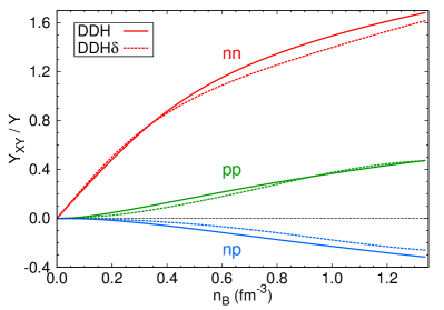
Figure 1: Entrainment coefficients $Y_{X\!Y}$ as functions of total baryon density $n_{B}$. Solid (dashed) lines refer to DDH($\delta$) EoS. Following the prescription given by Gusakov et al. Gusakov et al. (2009a), these coefficients are normalized to the constant $Y=3n_{0}/\mu^{\operatorname{\text{n}}}(3n_{0})$, where $n_{0}=0.16$ fm^-3 stands for the saturation density. For DDH($\delta$), $Y=2.55\times 10^{41}$ erg^-1.cm^-3 ($Y=2.47\times 10^{41}$ erg^-1.cm^-3).

Entrainment effects are depicted by the scalar $\alpha$ (18) which vanishes in the limit where there is no entrainment. As we do not take the presence of the crust into account in our model, entrainment is assumed to be only due to the strong interactions between nucleons. Two different approaches are commonly followed in the literature to quantify entrainment within the EoS: either by means of the entrainment matrix coefficients (Gusakov et al., 2009a) or by introducing dynamical effective masses (Chamel and Haensel, 2006).

The elements of the entrainment matrix, ${\mathcal{K}}^{X\!Y}$, and of its inverse, $\mathcal{Y}_{X\!Y}$, are functions of three quantities, e.g. $n_{\operatorname{\text{n}}},n_{\operatorname{\text{p}}}$ and $\Delta^{2}$. In order to compare entrainment effects within different EoSs, it is therefore convenient to study the limiting case of corotation (i.e. $\Delta^{2}=0$) with $\beta$-equilibrium (see Sec. II.3). We therefore introduce the entrainment coefficients (Gusakov et al., 2009a)

$$Y_{X\!Y}\equiv\mathcal{Y}_{X\!Y}|_{\Delta^{2}=0,\ \mu^{\operatorname{\text{n}}}=\mu^{\operatorname{\text{p}}}}~{},$$ (75)

which depend on a single parameter, e.g. the total baryon density $n_{B}=n_{\operatorname{\text{n}}}+n_{\operatorname{\text{p}}}$. These coefficients are plotted as functions of $n_{B}$ in Fig. 1, for both EoSs.

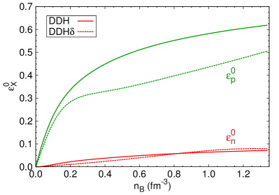
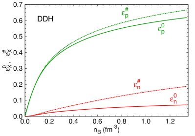
Figure 2: Left: Influence of the interaction on the entrainment parameters $\varepsilon_{X}^{0}$ . Solid (resp. dashed) lines refer to DDH($\delta$) EoS. For better clarity, only quantities defined in the zero-velocity frames are plotted. Right: Comparison between entrainment parameters defined in the zero-velocity frames ($\varepsilon_{X}^{0}$, solid lines) and in the zero-momentum frames ($\varepsilon_{X}^{\#}$, dashed lines), for the DDH EoS.

In order to study the importance of entrainment effects, we can also introduce dynamical effective masses. The idea is to describe the dynamics of each species as if it was alone. Interactions with the other fluid are included through the effective mass $\tilde{m}_{X}$ defined as

$$p_{X}^{\ i}=\tilde{m}_{X}\ u_{X}^{\ i},$$ (76)

where $p_{X}^{\ i}$ and $u_{X}^{\ i}$ stand for the spatial parts of the conjugate momentum and the 4-velocity of fluid $X$, respectively. Such a definition is formulated in the rest-frame of the background, i.e. the second fluid $Y$.

As already noticed by Prix et al. Prix et al. (2002), it is not possible to define the rest frame for fluid $Y$ in a unique way. In the zero-velocity frame of the fluid $Y$, where $u_{Y}^{\ i}=(0,0,0)$, Eq. (7) becomes

$$p_{X}^{\ i}=\mathcal{K}^{X\!X}n_{X}\ u_{X}^{\ i},$$ (77)

such that, using (13), we obtain

$$\tilde{m}_{X}=\mathcal{K}^{X\!X}n_{X}=\mu^{X}\left(1-\varepsilon_{X}\right),$$ (78)

where we have introduced the quantity

$$\varepsilon_{X}=\frac{2\alpha}{n_{X}\mu^{X}\Gamma_{\Delta}^{2}}.$$ (79)

Assuming again corotation and $\beta$-equilibrium, the following effective mass can be introduced (Prix et al., 2002; Chamel and Haensel, 2006)

$$m^{0}_{X}\equiv\operatorname{\mathcal{K}}^{XX}|_{\Delta^{2}=0,\ \mu^{\operatorname{\text{n}}}=\mu^{\operatorname{\text{p}}}}\ n_{X}=\mu^{X}\left(1-\varepsilon_{X}^{0}\right),$$ (80)

where $\varepsilon^{0}_{X}=\varepsilon_{X}|_{\Delta^{2}=0,\ \mu^{\operatorname{\text{n}}}=\mu^{\operatorname{\text{p}}}}$. In the zero-momentum frame of the fluid $Y$, where $p_{Y}^{\ i}=(0,0,0)$, Eq. (7) leads to

$$p_{X}^{\ i}=\frac{n_{X}}{\mathcal{Y}_{X\!X}}\ u_{X}^{\ i},$$ (81)

from which, we obtain

$$\tilde{m}_{X}=\frac{n_{X}}{\mathcal{Y}_{X\!X}}=\mu^{X}\left(1-\varepsilon_{X}\frac{1-\varepsilon_{Y}\Delta^{2}}{1-\varepsilon_{Y}}\right).$$ (82)

This leads us to introduce another effective mass for fluid $X$ (Prix et al., 2002; Chamel and Haensel, 2006)

$$m^{\#}_{X}\equiv\frac{n_{X}}{Y_{XX}}=\mu^{X}\left(1-\varepsilon_{X}^{\#}\right),$$ (83)

where

$$\varepsilon_{X}^{\#}=\frac{\varepsilon^{0}_{X}}{1-\varepsilon^{0}_{Y}}.$$ (84)

The quantities $m_{\operatorname{\text{n}}}^{0}$ and $m_{\operatorname{\text{n}}}^{\#}$ introduced so far are linked to the quantities $\varepsilon_{\text{mom}}$ and $\varepsilon_{\text{vel}}$ studied by Comer and Joynt (2003) through

$$m_{\operatorname{\text{n}}}^{0}=\varepsilon_{\text{vel}}m_{\operatorname{\text{n}}}\ \ \text{and}\ \ m_{\operatorname{\text{n}}}^{\#}=\frac{1}{\varepsilon_{\text{mom}}}m_{\operatorname{\text{n}}}.$$ (85)

The entrainment parameters $\varepsilon^{0}_{X}$ are shown in Fig. 2 - left, for the two different EoSs, as functions of the total baryon density. We do not show the dynamical masses since they contain not only entrainment effects, but also (special) relativistic corrections. In fact, for vanishing entrainment, i.e. $\alpha=0$, the effective masses (80) and (83) reduce to the chemical potentials (since all forms of energy contribute to the mass), not the bare masses. The parameters $\varepsilon_{X}$ are, on the contrary, a good measure of the importance of entrainment effects.

As can be seen in Fig. 2, entrainment effects become more and more important as the baryon density increases, where the interaction between particles gets stronger. Entrainment effects are quite important on the proton fluid beyond saturation density, whereas the neutron fluid is much less affected. This is simply a consequence of the relative proportion of the two fluids, $\varepsilon_{\operatorname{\text{n}}}=\frac{n_{\operatorname{\text{p}}}}{n_{\operatorname{\text{n}}}}\varepsilon_{p}$, when $\beta$-equilibrium is enforced. Note that we checked that the stability conditions derived by Chamel and Haensel (2006), i.e.

$$0\leq\varepsilon^{0}_{\operatorname{\text{n}}}<x_{\operatorname{\text{p}}}\ \ \text{and}\ \ 0\leq\varepsilon^{0}_{\operatorname{\text{p}}}<1-x_{\operatorname{\text{p}}},$$ (86)

where $x_{\operatorname{\text{p}}}=n_{\operatorname{\text{p}}}/n_{B}$, are verified. Results in the zero-momentum frame are very similar (see Fig. 2 - right), except at very high densities. The neutron fluid, anyway, is much less affected by entrainment and both parameters remain small with neutron effective masses close to $\mu^{\operatorname{\text{n}}}$. Comparing both EoSs, the general behavior is very similar. The discrepancy on the proton entrainment within the two EoSs, that is visible at high $n_{B}$, is due to the very different proton ratios (at $\beta$-equilibrium) predicted by these EoSs at a given $n_{B}$, as a consequence of the different values of symmetry energies and slopes at saturation density (see Table 1). As the neutrons are much more numerous, the influence of the different proton ratios on the neutron entrainment is smaller.

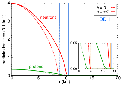
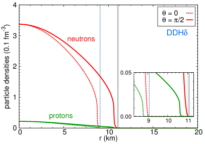
Figure 3: Density profiles $n_{\operatorname{\text{n}}}$ and $n_{\operatorname{\text{p}}}$ plotted with respect to the radial coordinate $r$ for a star with $M_{G}=1.4$ M_⊙ spinning at $\Omega_{\operatorname{\text{n}}}/2\pi=\Omega_{\operatorname{\text{p}}}/2\pi=716$ Hz, obtained with DDH and DDH$\delta$ EoSs. Neutron (protons) particle density $n_{\operatorname{\text{n}}}$ ($n_{\operatorname{\text{p}}}$) is plotted in red (green). Dashed and solid lines refer to profiles obtained in the polar and equatorial planes. Blue and orange vertical lines represent the coordinate of vanishing density of protons and neutrons. Some zooms of the area surrounding the surfaces are also presented.

IV Equilibrium configurations

We now use the model described in the previous sections to get some realistic equilibrium configurations describing superfluid neutron stars. Some general results were already discussed in Prix et al. Prix et al. (2005). Here, we mainly focus on the consequences of taking realistic EoSs into account.

For the different configurations studied in this Section, the virial identity violations (Gourgoulhon and Bonazzola, 1994; Bonazzola and Gourgoulhon, 1994), which are useful checks of the accuracy of numerical solutions of Einstein equations, are of the order of $\sim 10^{-8}-10^{-5}$ depending on the mass of the neutron star, the rotation rates and the choice of the grid used to describe the star. This means that the numerical errors in our models should be below this value and gives us confidence in the accuracy of our results.

IV.1 Density profiles

Assuming corotation and $\beta$-equilibrium, the external fluid appears to be always the proton fluid, because $m_{\operatorname{\text{p}}}~{}\lesssim~{}m_{\operatorname{\text{n}}}$. A more realistic model would consider the presence of an elastic crust below the surface of the star. For the DDH$\delta$ EoS, the maximum mass predicted is $2.16$ M_⊙ in the static case and increases up to $2.21$ M_⊙ for 716 Hz, the highest rotation frequency observed today Hessels et al. (2006). The maximum masses obtained with the DDH EoS are a bit smaller: $2.08$ M_⊙ for static configurations and $2.12$ M_⊙ at 716 Hz. These values are consistent with the accurate measurements of 2 M_⊙ neutron stars in binary pulsars (Demorest et al., 2010; Antoniadis et al., 2013). We refrain from giving radius values here, since our model does not contain any elastic crust, inducing an error of the order 500 m in the radius determination.

Keeping $\beta$-equilibrium at the center of the star, and allowing for a relative lag of up to $\left(\Omega_{\operatorname{\text{n}}}-\Omega_{\operatorname{\text{p}}}\right)/\Omega_{\operatorname{\text{p}}}\sim 1.4\times 10^{-3}$, the relative increase of the maximum mass is $\sim 6\times 10^{-5}$. Such a lag is well beyond the maximum lag expected in neutron stars from the glitch amplitude (see footnote in Sec. II.3). We thus conclude that the maximum mass is very precisely determined in the corotation approximation.

Assuming again corotation and $\beta$-equilibrium, we plot the density profiles obtained from the two EoSs as functions of the radial coordinate $r$ in Fig. 3 for a star whose gravitational mass is $1.4$ M_⊙, with a rotation rate $\Omega_{\operatorname{\text{n}}}/2\pi=\Omega_{\operatorname{\text{p}}}/2\pi=716$ Hz. Profiles in the equatorial (polar) planes are shown in solid (dashed) lines. It can be nicely seen in the zoom (right panel) that the proton fluid is the external fluid. As expected, protons are much less abundant than neutrons. At the center of the star ($r=0$), the proton ratio is $x_{\operatorname{\text{p}}}=n_{\operatorname{\text{p}}}/n_{B}\simeq 0.08$ for the DDH EoS, whereas $x_{\operatorname{\text{p}}}(r=0)\simeq 0.06$ for the DDH$\delta$ EoS. Using the DDH EoS, the central baryon density is equal to $n_{B}(r=0)\simeq 0.44$ fm^-3, which is close to three times the saturation density. With the DDH$\delta$ EoS, it is smaller, $n_{B}(r=0)\simeq 0.36$ fm^-3. The difference comes from the fact that for $\beta$-equilibrated matter at a given $n_{B}$ relevant for neutron stars, as can be inferred from symmetry energy and slope the pressure is systematically higher in DDH$\delta$ than in DDH. Therefore, for the same gravitational mass of the star, $n_{B}$ is lower. Here we do not study the influence of a difference in rotation rates between both fluids because from the astrophysical side it is expected to be so small that the results would be very similar to those presented in Fig. 3 and, on the other hand, many results concerning models with arbitrarily different rotation rates were presented in Prix et al. Prix et al. (2005).

IV.2 Angular momenta

We give here some results on the angular momenta, as well as for moments of inertia defined in Sec. II.4. The moments of inertia $I$, $I_{\operatorname{\text{n}}}$ and $I_{\operatorname{\text{p}}}$ are plotted as functions of the angular velocity of the star in Fig. 4, assuming $\Omega_{\operatorname{\text{n}}}=\Omega_{\operatorname{\text{p}}}$. Here is considered a sequence with constant total baryon mass, corresponding to neutron stars whose gravitational masses are around $1.4$ M_⊙. At low angular velocities, the moments of inertia are nearly constant, such that the angular momenta depend linearly on $\Omega_{X}$. Approaching Keplerian velocity, this is no longer the case and momenta of inertia and angular momenta are steeply increasing. As expected, the total angular momentum of the star is dominated by the neutron angular momentum.

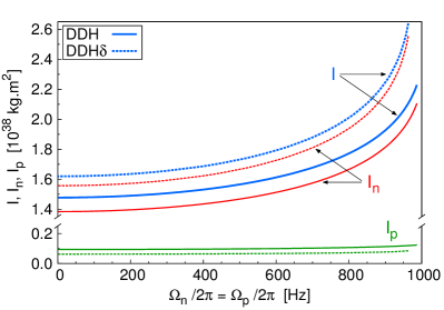
Figure 4: Moments of inertia plotted with respect to the angular velocity of the pulsar, taking both angular velocities to be equal and assuming $\beta$-equilibrium, for a (same) fixed total baryon mass $M^{B}=1.542$ M_⊙ corresponding to $M_{G}\simeq 1.4$ M_⊙. Results from the DDH (DDH$\delta$) EoS are represented with solid (dashed) lines. Total quantities are shown in blue whereas neutron (proton) ones are plotted in red (green).

Note that in the present two-fluid case the angular momentum of a fluid can be nonzero even if its angular velocity vanishes. Two different effects can be identified at the origin of this phenomenon. The first one is the general relativistic frame-dragging effect, which can be seen through the presence of the metric term $\omega$ in the definition of the physical velocities (cf. Eq. (23)). Although $\Omega_{\operatorname{\text{p}}}=0$, the rotation of the neutron fluid ($\Omega_{\operatorname{\text{n}}}\neq 0$) thus leads to $U_{\operatorname{\text{p}}}<0$ and to a non-vanishing proton angular momentum (see (38) and (39)). The second contribution refers to the dependence of the proton angular momentum on the physical velocity of the neutron fluid as a consequence of entrainment (see e.g. (87)), which is clearly visible on Eq. (94) in the Newtonian limit. To illustrate this phenomenon, in Fig. 5 two sequences of stars (corresponding to the two EoSs) are plotted as a function of $\Omega_{\operatorname{\text{n}}}$, assuming $\Omega_{\operatorname{\text{p}}}=0$ Hz, for a fixed baryon mass. Although the proton angular velocity vanishes, its angular momentum is nonzero, rising roughly linearly with $\Omega_{\operatorname{\text{n}}}$. Entrainment gives thereby the dominant contribution, since $J_{\operatorname{\text{p}}}$ is positive, but the frame-dragging effect (which acts on the proton angular momentum in an opposite way to entrainment) contributes almost as much as entrainment.

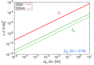
Figure 5: Neutron and proton angular momenta as functions of the neutron angular velocity $\Omega_{\operatorname{\text{n}}}$, assuming the proton fluid to be at rest with respect to a static observer at spatial infinity ($\Omega_{\operatorname{\text{p}}}/2\pi=0$ Hz). Results from the DDH (DDH$\delta$) EoS are shown with solid (dashed) lines. Quantities are plotted for a fixed total baryon mass (equal for the two EoSs), assuming $\beta$-equilibrium at the center.

V Conclusion

Both microscopic calculations and observations give strong indications that the interior of neutrons stars contains superfluid matter. Superfluidity is thus an important ingredient that needs to be taken into account in order to build realistic models for neutron stars, which could be very useful for the study of oscillations, glitches and cooling phenomena.

As a first step towards this objective, we have extended the numerical model of stationary rotating superfluid neutron stars proposed by Prix et al. Prix et al. (2005) to the use of realistic EoS. These models consider the neutron star to be composed of two fluids, neutrons and charged particles (protons and electrons), which are free to rotate uniformly around a common axis with different angular velocities. Obviously, these models can be applied for any rotation frequency and go therefore beyond the slow rotation approximation models of Refs. Andersson and Comer (2001); Comer (2004); Kheto and Bandyopadhyay (2015). To reach high numerical accuracy, tabulated two-fluid EoSs were interpolated with a high-order thermodynamically consistent scheme, that we tested on analytic EoSs. An overall precision of $10^{-7}$-$10^{-8}$, measured via violations of the virial theorem, could be reached. This is of the same order as typical one-fluid models employing realistic EoS. These are first numerical model of rapidly rotating neutron stars in full general relativity and with realistic EoSs.

For these numerical models we need the EoS depending on the two densities and the relative velocity, i.e. $\operatorname{\mathcal{E}}(n_{n},n_{p},\Delta^{2})$. To this end, following the spirit of Comer and Joynt Comer and Joynt (2003), we have presented a formalism to calculate the EoS at an arbitrary value of $\Delta^{2}$. Entrainment parameters have been derived from this EoS. We have shown that in the limit of small $\Delta^{2}$ our entrainment parameters are in agreement with those derived from Fermi liquid theory to lowest order in the relative velocities. This means that the large numerical differences between the entrainment parameters calculated on the one hand in Refs. Comer and Joynt (2003); Kheto and Bandyopadhyay (2014, 2015) from the EoS and on the other hand in Refs. Gusakov et al. (2009a, 2014) from Fermi liquid theory simply stem from the fact that the relativistic deformation of the Fermi spheres has not been taken into account in the calculations of Refs. Comer and Joynt (2003); Kheto and Bandyopadhyay (2014, 2015). We have applied our new formalism to two density-dependent RMF parametrizations, DDH and DDH$\delta$, being consistent with standard nuclear matter and neutron star properties. The entrainment parameters are qualitatively very similar in both models. If $\beta$-equilibrium is imposed, entrainment has a stronger effect on the proton fluid due to the low proton fraction. Quantitatively, the difference between both models is non-negligible only for the proton fluid, the higher proton fraction in DDH leading to more pronounced entrainment effects than in DDH$\delta$.

As a first application, we have computed several relativistic equilibrium configurations. As expected, maximum masses are only marginally influenced by entrainment and a small lag in rotation frequencies of the two fluids. We did not discuss radii since our models do not contain any crust, and the extracted radii would thus not be reliable. Entrainment is more important for the determination of angular momenta and moment of inertia. In particular, the angular momentum of one fluid can be nonzero even if its angular velocity is vanishing. The entrainment induces thereby an opposite effect to relativistic frame dragging. We have shown that with our EoS, entrainment is slightly more important than frame-dragging, leading to a positive angular momentum for the non-rotating fluid.

In this paper, we mainly focused on the properties of neutron stars cores assuming homogeneous matter. As already mentioned before, entrainment effects are expected to be much stronger in the solid crust due to Bragg scattering of dripped neutrons off nuclear clusters Chamel (2005, 2012). An interesting extension of this work would thus be to include the presence of a solid crust. We also plan to use the models discussed here for the study of quasi-stationary evolution of neutron stars, as could be found during glitches.

Appendix A Newtonian limit of the angular momenta

Here, we study the Newtonian limit of Eqs. (38) and (39). To do so, we rewrite the two angular momentum densities as

$$\left\{\begin{array}[]{rcl}j^{\operatorname{\text{n}}}_{\varphi}&=&\left[n_{\operatorname{\text{n}}}\Gamma_{\operatorname{\text{n}}}^{2}\mu^{\operatorname{\text{n}}}\ U_{\operatorname{\text{n}}}+2\alpha\frac{\Gamma_{\operatorname{\text{n}}}^{2}}{\Gamma_{\Delta}^{2}}\left(\frac{\Gamma_{\operatorname{\text{p}}}}{\Gamma_{\Delta}\Gamma_{\operatorname{\text{n}}}}U_{\operatorname{\text{p}}}-U_{\operatorname{\text{n}}}\right)\right]Br\sin\theta,\\[5.0pt] j^{\operatorname{\text{p}}}_{\varphi}&=&\left[n_{\operatorname{\text{p}}}\Gamma_{\operatorname{\text{p}}}^{2}\mu^{\operatorname{\text{p}}}\ U_{\operatorname{\text{p}}}+2\alpha\frac{\Gamma_{\operatorname{\text{p}}}^{2}}{\Gamma_{\Delta}^{2}}\left(\frac{\Gamma_{\operatorname{\text{n}}}}{\Gamma_{\Delta}\Gamma_{\operatorname{\text{p}}}}U_{\operatorname{\text{n}}}-U_{\operatorname{\text{p}}}\right)\right]Br\sin\theta.\end{array}\right.$$ (87)

In the Newtonian limit, the different quantities appearing in Eq. (87) simplify as $\Gamma_{\operatorname{\text{n}}}\simeq\Gamma_{\operatorname{\text{p}}}\simeq\Gamma_{\Delta}\simeq 1$, $\mu^{\operatorname{\text{n}}}\simeq m_{\operatorname{\text{n}}}$ and $\mu^{\operatorname{\text{p}}}\simeq m_{\operatorname{\text{p}}}$. Thus, Eq. (87) becomes

$$\left\{\begin{array}[]{rcl}j^{\operatorname{\text{n}}}_{\varphi}&=&\left[n_{\operatorname{\text{n}}}m_{\operatorname{\text{n}}}\ U_{\operatorname{\text{n}}}+2\alpha\left(U_{\operatorname{\text{p}}}-U_{\operatorname{\text{n}}}\right)\right]r\sin\theta,\\[3.0pt] j^{\operatorname{\text{p}}}_{\varphi}&=&\left[n_{\operatorname{\text{p}}}m_{\operatorname{\text{p}}}\ U_{\operatorname{\text{p}}}+2\alpha\left(U_{\operatorname{\text{n}}}-U_{\operatorname{\text{p}}}\right)\right]r\sin\theta,\end{array}\right.$$ (88)

where the physical velocities verify

$$U_{\operatorname{\text{n}}}\simeq\Omega_{\operatorname{\text{n}}}r\sin\theta\ \ \text{and}\ \ U_{\operatorname{\text{p}}}\simeq\Omega_{\operatorname{\text{p}}}r\sin\theta.$$ (89)

Considering that $A\rightarrow 1$ and $B\rightarrow 1$, the element volume $\operatorname{\mathrm{d}\!}^{\,3}\!\Sigma$ tends towards $\operatorname{\mathrm{d}\!}^{\,3}\!\Sigma_{\text{f}}=r^{2}\sin\theta\operatorname{\mathrm{d}\!}r\operatorname{\mathrm{d}\!}\theta\operatorname{\mathrm{d}\!}\varphi$, which is the element volume of the flat spacetime. Replacing Eq. (88) in Eq. (39), the non relativistic limit of the angular momentum of the two fluids reads as

$$\left\{\begin{array}[]{rcl}J_{\operatorname{\text{n}}}&=&\int_{\Sigma_{t}}n_{\operatorname{\text{n}}}m_{\operatorname{\text{n}}}\left(\Omega_{\operatorname{\text{n}}}+\varepsilon_{\operatorname{\text{n}}}\left(\Omega_{\operatorname{\text{p}}}-\Omega_{\operatorname{\text{n}}}\right)\right)r^{2}\sin^{2}\theta\operatorname{\mathrm{d}\!}^{\,3}\!\Sigma_{\text{f}},\\[3.0pt] J_{\operatorname{\text{p}}}&=&\int_{\Sigma_{t}}n_{\operatorname{\text{p}}}m_{\operatorname{\text{p}}}\left(\Omega_{\operatorname{\text{p}}}+\varepsilon_{\operatorname{\text{p}}}\left(\Omega_{\operatorname{\text{n}}}-\Omega_{\operatorname{\text{p}}}\right)\right)r^{2}\sin^{2}\theta\operatorname{\mathrm{d}\!}^{\,3}\!\Sigma_{\text{f}},\end{array}\right.$$ (90)

where the entrainment parameters $\varepsilon_{\operatorname{\text{n}}}$ and $\varepsilon_{\operatorname{\text{p}}}$ are defined as

$$\varepsilon_{\operatorname{\text{n}}}n_{\operatorname{\text{n}}}m_{\operatorname{\text{n}}}=2\alpha=\varepsilon_{\operatorname{\text{p}}}n_{\operatorname{\text{p}}}m_{\operatorname{\text{p}}},$$ (91)

see Eq. (79). Assuming the two angular velocities to be uniform and introducing the moment of inertia of fluid $X$

$$I_{X}=\displaystyle\int_{\Sigma_{t}}n_{X}m_{X}r^{2}\sin^{2}\theta\operatorname{\mathrm{d}\!}^{\,3}\!\Sigma_{\text{f}},$$ (92)

and its corresponding mean coupling term

$$\tilde{\varepsilon}_{X}=\frac{\displaystyle\int_{\Sigma_{t}}\varepsilon_{X}n_{X}m_{X}r^{2}\sin^{2}\theta\operatorname{\mathrm{d}\!}^{\,3}\!\Sigma_{\text{f}}}{\displaystyle\int_{\Sigma_{t}}n_{X}m_{X}r^{2}\sin^{2}\theta\operatorname{\mathrm{d}\!}^{\,3}\!\Sigma_{\text{f}}},$$ (93)

the two Newtonian angular momenta read as

$$\left\{\begin{array}[]{rcl}J_{\operatorname{\text{n}}}&=&I_{\operatorname{\text{n}}}\Omega_{\operatorname{\text{n}}}+I_{\operatorname{\text{n}}}\tilde{\varepsilon}_{\operatorname{\text{n}}}\left(\Omega_{\operatorname{\text{p}}}-\Omega_{\operatorname{\text{n}}}\right),\\[3.0pt] J_{\operatorname{\text{p}}}&=&I_{\operatorname{\text{p}}}\Omega_{\operatorname{\text{p}}}+I_{\operatorname{\text{p}}}\tilde{\varepsilon}_{\operatorname{\text{p}}}\left(\Omega_{\operatorname{\text{n}}}-\Omega_{\operatorname{\text{p}}}\right),\end{array}\right.$$ (94)

in agreement with the results by Sidery et al. Sidery et al. (2010).

Appendix B Numerical implementation of the tabulated EoS

Considering a tabulated EoS leads to two additional kinds of numerical errors, linked to the accuracy with which the table is computed and the precision of the interpolation scheme.

For each iteration step in the numerical procedure, the matter sources involved in the Einstein equations are computed from the values of $H^{\operatorname{\text{n}}}$, $H^{\operatorname{\text{p}}}$ and $\Delta^{2}$ at every grid points (see Prix et al. (2005)). We then use the EoS in the form of the pressure $\Psi(\mu^{\operatorname{\text{n}}},\mu^{\operatorname{\text{p}}},\Delta^{2})$ (cf. Eq. (16)), instead of the energy density $\operatorname{\mathcal{E}}$. For each EoS, we build a table using a grid made of parallelepipeds in the relative speed $\Delta^{2}$ and the chemical potentials $\mu^{\operatorname{\text{n}}}$ and $\mu^{\operatorname{\text{p}}}$ (see Fig. 6), which contains, for a given value of this triplet, the set of variables required to the interpolation. As the different thermodynamic quantities can be expressed as functions of the interpolated values of $\Psi$, $n_{\operatorname{\text{n}}}$, $n_{\operatorname{\text{p}}}$ and $\alpha$ (cf. Eqs. (13) and (14)), we need a scheme able to interpolate with high precision a function and its first derivatives (cf. Eqs. (17) and (18)).

To do so, we use the thermodynamically consistent interpolation based on Hermit polynomials presented by Swesty (1996). Unfortunately, one can not directly employ this high-order method on the triplet $(\mu^{\operatorname{\text{n}}},\mu^{\operatorname{\text{p}}},\Delta^{2})$, because it would require the presence of 3-order derivatives in the table, which are extremely difficult to compute with sufficient precision. Instead, the 3D interpolation scheme we implemented is the following (see Fig.6):

1. One starts by locating in the table the triplet $\left(\Delta^{2},\mu^{\operatorname{\text{n}}},\mu^{\operatorname{\text{p}}}\right)$ in which the interpolation is required,

2. On the two planes with constant $\Delta^{2}$ surrounding this point, we carry out a 2D thermodynamically consistent interpolation in the chemical potentials on $\Psi$ (which also gives the values of $n_{\operatorname{\text{n}}}$ and $n_{\operatorname{\text{p}}}$) and on $\alpha$,

3. We use a linear interpolation in the $\Delta^{2}$ dimension on $\Psi$, $n_{\operatorname{\text{n}}}$, $n_{\operatorname{\text{p}}}$ and $\alpha$.

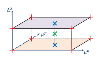
Figure 6: 3D interpolation scheme on a parallelepipedic grid (red crosses), in a point corresponding to a given value of $(\Delta^{2},\mu^{\operatorname{\text{n}}},\mu^{\operatorname{\text{p}}})$ (green cross). On each plan where $\Delta^{2}$ is constant, quantities are interpolated with a 2D thermodynamically consistent method on the chemical potentials (blue crosses). From these two values, a linear interpolation is used in $\Delta^{2}$, in order to obtain the values of the quantities needed at the interesting point.

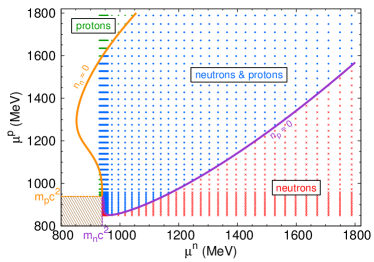
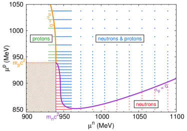
Figure 7: Single-fluid (red crosses and green triangles) and two-fluid (blue dots) areas in the plane $(\mu^{\operatorname{\text{n}}},\mu^{\operatorname{\text{p}}})$, for $\Delta^{2}=0$, using the DDH$\delta$ EoS. The two-fluid zone is delimited by the limit lines $n_{\operatorname{\text{n}}}=0$ (orange) and $n_{\operatorname{\text{p}}}=0$ (purple), beyond which one fluid disappears. For chemical potentials below the rest masses $m_{\operatorname{\text{n}}}=939.6$ MeV and $m_{\operatorname{\text{p}}}=938.8$ MeV no fluid is present, as can be seen on the zoom shown on the right. Note that $m_{\operatorname{\text{p}}}$ denotes here the sum of the rest mass of protons and that of electrons since the subscript $p$ stands here for fluid of charged particles. For better clarity, only a small proportion of the data contained in the table is plotted. In order to describe the area at low densities, where rapid variations occur, one uses a refined mesh. As realistic configurations are expected to be close to $\beta$-equilibrium and corotation, only the data around the $\mu^{\operatorname{\text{n}}}=\mu^{\operatorname{\text{p}}}$ line will be used.

To use the 2D interpolation method in 2., it is necessary to provide some values of the function, its two derivatives and the cross-derivative in the table. In the case of $\alpha$, this cross-derivative would be a third-order derivative in $\Psi$, that can not be provided with a good precision. Thus, for simplicity, we employ the same interpolation scheme for $\Psi$ and $\alpha$, without considering the cross-derivative in the second case. The precision on the global interpolation scheme remains sufficiently good. Note that we simply used a linear interpolation in the relative speed because the data provided in the table are computed with a first-order method. No derivatives with respect to $\Delta^{2}$ are thus required in the table.

We studied the consistency of this interpolation scheme by comparing the results given by the code using directly an analytic EoS, as was studied in (Prix et al., 2005), and by the same code interpolating a table based on the same EoS (computed with machine-precision). The relative difference in the numerical results obtained within these two methods were found to be very small.

A part of the DDH$\delta$ table, corresponding to the $\Delta^{2}=0$ plane, is shown in Fig. 7. The different areas in which protons and/or neutrons are present are displayed. As can be seen in Fig. 7, neutrons (and protons) can appear in the system for values of the chemical potential below the corresponding rest mass, as a consequence of the strong interactions between nucleons (see Sec. III).

References

- Comer and Joynt (2003) G. L. Comer and R. Joynt, Physical Review D 68, 023002 (2003).
- Haensel et al. (2007) P. Haensel, A. Y. Potekhin, and D. G. Yakovlev, Neutron stars 1: Equation of state and structure, Vol. 326 (Springer Science & Business Media, 2007).
- Migdal (1959) A. B. Migdal, Nuclear Physics 13, 655 (1959).
- Dean and Hjorth-Jensen (2003) D. J. Dean and M. Hjorth-Jensen, Reviews of Modern Physics 75, 607 (2003).
- Gnedin et al. (2001) O. Y. Gnedin, D. G. Yakovlev, and A. Y. Potekhin, Monthly Notices of the Royal Astronomical Society 324, 725 (2001).
- Anderson and Itoh (1975) P. W. Anderson and N. Itoh, Nature 256, 25 (1975).
- Alpar et al. (1984a) M. A. Alpar, D. Pines, P. W. Anderson, and J. Shaham, The Astrophysical Journal 276, 325 (1984a).
- Haskell et al. (2012) B. Haskell, P. M. Pizzochero, and T. Sidery, Monthly Notices of the Royal Astronomical Society 420, 658 (2012).
- Wong et al. (2001) T. Wong, D. C. Backer, and A. G. Lyne, The Astrophysical Journal 548, 447 (2001).
- Espinoza et al. (2011) C. M. Espinoza, A. G. Lyne, B. W. Stappers, and M. Kramer, Monthly Notices of the Royal Astronomical Society 414, 1679 (2011).
- Haskell and Melatos (2015) B. Haskell and A. Melatos, International Journal of Modern Physics D 24 (2015).
- Heinke and Ho (2010) C. O. Heinke and W. C. G. Ho, The Astrophysical Journal Letters 719, L167 (2010).
- Shternin et al. (2011) P. S. Shternin, D. G. Yakovlev, C. O. Heinke, W. C. G. Ho, and D. J. Patnaude, Monthly Notices of the Royal Astronomical Society: Letters 412, L108 (2011).
- Page et al. (2011) D. Page, M. Prakash, J. M. Lattimer, and A. W. Steiner, Physical Review Letters 106, 081101 (2011).
- Strohmayer and Watts (2006) T. E. Strohmayer and A. L. Watts, The Astrophysical Journal 653, 593 (2006).
- Gabler et al. (2013) M. Gabler, P. Cerdá-Durán, N. Stergioulas, J. A. Font, and E. Müller, Physical review letters 111, 211102 (2013).
- Baym et al. (1969) G. Baym, C. Pethick, and D. Pines, Nature 224, 673 (1969).
- Alpar et al. (1984b) M. A. Alpar, S. A. Langer, and J. A. Sauls, The Astrophysical Journal 282, 533 (1984b).
- Chamel (2008) N. Chamel, Monthly Notices of the Royal Astronomical Society 388, 737 (2008).
- Chamel (2005) N. Chamel, Nuclear Physics A 747, 109 (2005).
- Chamel (2012) N. Chamel, Physical Review C 85, 035801 (2012).
- Andersson et al. (2002) N. Andersson, G. L. Comer, and D. Langlois, Physical Review D 66, 104002 (2002).
- Haskell et al. (2009) B. Haskell, N. Andersson, and A. Passamonti, Monthly Notices of the Royal Astronomical Society 397, 1464 (2009).
- Andersson et al. (2012) N. Andersson, K. Glampedakis, W. C. G. Ho, and C. M. Espinoza, Physical review letters 109, 241103 (2012).
- Chamel (2013) N. Chamel, Physical review letters 110, 011101 (2013).
- Carter (1989) B. Carter, Lecture Notes in Mathematics, Berlin Springer Verlag 1385, 1 (1989).
- Carter and Langlois (1998) B. Carter and D. Langlois, Nuclear Physics B 531, 478 (1998).
- Langlois et al. (1998) D. Langlois, D. M. Sedrakian, and B. Carter, Monthly Notices of the Royal Astronomical Society 297, 1189 (1998).
- Andersson and Comer (2001) N. Andersson and G. L. Comer, Classical and Quantum Gravity 18, 969 (2001).
- Comer (2004) G. L. Comer, Physical Review D 69, 123009 (2004).
- Gusakov et al. (2009a) M. E. Gusakov, E. M. Kantor, and P. Haensel, Physical Review C 79, 055806 (2009a).
- Kheto and Bandyopadhyay (2014) A. Kheto and D. Bandyopadhyay, Physical Review D 89, 023007 (2014).
- Kheto and Bandyopadhyay (2015) A. Kheto and D. Bandyopadhyay, Physical Review D 91, 043006 (2015).
- Prix et al. (2005) R. Prix, J. Novak, and G. L. Comer, Physical Review D 71, 043005 (2005).
- Hessels et al. (2006) J. W. T. Hessels, S. M. Ransom, I. H. Stairs, P. C. C. Freire, V. M. Kaspi, and F. Camilo, Science 311, 1901 (2006).
- Typel and Wolter (1999) S. Typel and H. H. Wolter, Nuclear Physics A 656, 331 (1999).
- Avancini et al. (2009) S. S. Avancini, L. Brito, J. R. Marinelli, D. P. Menezes, M. M. W. de Moraes, C. Providência, and A. M. Santos, Physical Review C 79, 035804 (2009).
- Carter et al. (2005) B. Carter, N. Chamel, and P. Haensel, Nuclear Physics A 748, 675 (2005).
- Carter et al. (2006) B. Carter, N. Chamel, and P. Haensel, International Journal of Modern Physics D 15, 777 (2006).
- Carter and Samuelsson (2006) B. Carter and L. Samuelsson, Classical and Quantum Gravity 23, 5367 (2006).
- Friedman and Stergioulas (2013) J. L. Friedman and N. Stergioulas, Rotating Relativistic Stars (Cambridge University Press, 2013).
- Gusakov et al. (2009b) M. E. Gusakov, E. M. Kantor, and P. Haensel, Phys. Rev. C80, 015803 (2009b).
- Easson (1979) I. Easson, The Astrophysical Journal 228, 257 (1979).
- Glampedakis and Lasky (2015) K. Glampedakis and P. D. Lasky, Monthly Notices of the Royal Astronomical Society 450, 1638 (2015).
- Chatterjee et al. (2015) D. Chatterjee, T. Elghozi, J. Novak, and M. Oertel, Monthly Notices of the Royal Astronomical Society 447, 3785 (2015).
- Bonazzola et al. (1993) S. Bonazzola, E. Gourgoulhon, M. Salgado, and J. A. Marck, Astronomy and Astrophysics 278, 421 (1993).
- Shapiro (2000) S. L. Shapiro, The Astrophysical Journal 544, 397 (2000).
- Flowers and Itoh (1976) E. Flowers and N. Itoh, The Astrophysical Journal 206, 218 (1976).
- Hegyi (1977) D. J. Hegyi, The Astrophysical Journal 217, 244 (1977).
- Andreev and Bashkin (1976) A. F. Andreev and E. P. Bashkin, Soviet Journal of Experimental and Theoretical Physics 42, 164 (1976).
- Gourgoulhon (2012) E. Gourgoulhon, 3+ 1 formalism in general relativity: bases of numerical relativity, Vol. 846 (Springer Science & Business Media, 2012).
- Prix et al. (2002) R. Prix, G. L. Comer, and N. Andersson, Astronomy & Astrophysics 381, 178 (2002).
- Yakovlev et al. (2001) D. G. Yakovlev, A. D. Kaminker, O. Y. Gnedin, and P. Haensel, Physics Reports 354, 1 (2001).
- Sidery et al. (2010) T. Sidery, A. Passamonti, and N. Andersson, Monthly Notices of the Royal Astronomical Society 405, 1061 (2010).
- Komar (1959) A. Komar, Physical Review 113, 934 (1959).
- Grandclément and Novak (2009) P. Grandclément and J. Novak, Living Rev. Relativity 12 (2009).
- Glendenning (2000) N. K. Glendenning, Compact stars: Nuclear physics, particle physics and general relativity (Springer, 2000).
- Dutra et al. (2014) M. Dutra, O. Lourenço, S. S. Avancini, B. V. Carlson, A. Delfino, D. P. Menezes, C. Providência, S. Typel, and J. R. Stone, Physical Review C 90, 055203 (2014).
- Gaitanos et al. (2004) T. Gaitanos, M. Di Toro, S. Typel, V. Baran, C. Fuchs, V. Greco, and H. H. Wolter, Nuclear Physics A 732, 24 (2004).
- Avancini et al. (2004) S. S. Avancini, L. Brito, D. P. Menezes, and C. Providência, Physical Review C 70, 015203 (2004).
- Urban and Oertel (2015) M. Urban and M. Oertel, International Journal of Modern Physics E 24, 1541006 (2015).
- Krüger et al. (2013) T. Krüger, I. Tews, K. Hebeler, and A. Schwenk, Physical Review C 88, 025802 (2013).
- Danielewicz and Lee (2009) P. Danielewicz and J. Lee, Nuclear Physics A 818, 36 (2009).
- Piekarewicz (2010) J. Piekarewicz, Journal of Physics G: Nuclear and Particle Physics 37, 064038 (2010).
- Tsang et al. (2012) M. B. Tsang, J. R. Stone, F. Camera, P. Danielewicz, S. Gandolfi, K. Hebeler, C. J. Horowitz, J. Lee, W. G. Lynch, Z. Kohley, et al., Physical Review C 86, 015803 (2012).
- Lattimer and Lim (2013) J. M. Lattimer and Y. Lim, The Astrophysical Journal 771, 51 (2013).
- Lattimer and Steiner (2014) J. M. Lattimer and A. W. Steiner, The European Physical Journal A 50, 1 (2014).
- Typel et al. (2015) S. Typel, M. Oertel, and T. Klaehn, Physics of Particles and Nuclei 46, 633 (2015).
- Chamel and Haensel (2006) N. Chamel and P. Haensel, Physical Review C 73, 045802 (2006).
- Gusakov et al. (2014) M. E. Gusakov, P. Haensel, and E. M. Kantor, Monthly Notices of the Royal Astronomical Society 439, 318 (2014).
- Baym and Chin (1976) G. Baym and S. A. Chin, Nuclear Physics A 262, 527 (1976).
- Gusakov and Kantor (2013) M. E. Gusakov and E. M. Kantor, Mon. Not. Roy. Astron. Soc. 428, L26 (2013).
- Gourgoulhon and Bonazzola (1994) E. Gourgoulhon and S. Bonazzola, Classical and Quantum Gravity 11, 443 (1994).
- Bonazzola and Gourgoulhon (1994) S. Bonazzola and E. Gourgoulhon, Classical and Quantum Gravity 11, 1775 (1994).
- Demorest et al. (2010) P. B. Demorest, T. Pennucci, S. M. Ransom, M. S. E. Roberts, and J. W. T. Hessels, Nature 467, 1081 (2010).
- Antoniadis et al. (2013) J. Antoniadis, P. C. Freire, N. Wex, T. M. Tauris, R. S. Lynch, M. H. van Kerkwijk, M. Kramer, C. Bassa, V. S. Dhillon, T. Driebe, et al., Science 340, 1233232 (2013).
- Swesty (1996) F. D. Swesty, Journal of Computational Physics 127, 118 (1996).