STAR FORMATION IN W3 - AFGL333: YOUNG STELLAR CONTENT, PROPERTIES AND ROLES OF EXTERNAL FEEDBACK

Abstract

One of the key questions in the field of star formation is the role of stellar feedback on subsequent star formation process. The W3 giant molecular cloud complex at the western border of the W4 super bubble is thought to be influenced by the stellar winds of the massive stars in W4. AFGL333 is a $\sim$ 10⁴ $M_{\odot}$ cloud within W3. This paper presents a study of the star formation activity within AFGL333 using deep $JHK_{s}$ photometry obtained from the NOAO Extremely Wide-Field Infrared Imager combined with Spitzer-IRAC-MIPS photometry. Based on the infrared excess, we identify 812 candidate young stellar objects in the complex, of which 99 are classified as Class I and 713 are classified as Class II sources. The stellar density analysis of young stellar objects reveals three major stellar aggregates within AFGL333, named here AFGL333-main, AFGL333-NW1 and AFGL333-NW2. The disk fraction within AFGL333 is estimated to be $\sim$ 50–60%. We use the extinction map made from the $H-K_{s}$ colors of the background stars to understand the cloud structure and to estimate the cloud mass. The CO-derived extinction map corroborates the cloud structure and mass estimates from NIR color method. From the stellar mass and cloud mass associated with AFGL333, we infer that the region is currently forming stars with an efficiency of $\sim$ 4.5% and at a rate of $\sim$ 2 - 3 $M_{\odot}$ Myr^-1pc^-2. In general, the star formation activity within AFGL333 is comparable to that of nearby low mass star-forming regions. We do not find any strong evidence to suggest that the stellar feedback from the massive stars of nearby W4 super bubble has affected the global star formation properties of the AFGL333 region.

1. Introduction

Most stars form in OB associations, where stellar winds, UV radiation and supernova explosions from the massive members significantly affect their environment. Feedback from newly born massive stars plays an active role in the subsequent evolution of their parent molecular cloud. Feedback can trigger the birth of new generations of stars that would otherwise not exist, allowing star formation to propagate continuously from one point to the next (Elmegreen & Lada, 1977). On the other hand, feedback may also inhibit star formation by clearing away the dust and gas (Bisbas et al., 2011; Walch et al., 2013; Dale et al., 2013).

Numerical simulation studies by Dale & Bonnell (2012) and Dale et al. (2013) show that the effect of feedback in a massive star forming region depends on its cloud mass and density. The most massive and largest clouds are mostly dynamically unaffected by stellar feedback. On the other hand, feedback has a profound effect on the lower density clouds, expelling tens of percent of the neutral gas long before any massive star explode as a supernova. Since giant molecular clouds typically have complicated, clumpy internal structures, the stellar feedback mechanisms penetrate into different depths in different directions of a given cloud, producing highly irregular morphologies (Walch et al., 2013). The global influence of feedback on a given system may therefore differ from the local effects; star formation could be suppressed at some locations and triggered in another location (Dale & Bonnell, 2012).

The W3 star forming complex (d $\sim$ 2 kpc; Xu et al. 2006; Hachisuka et al. 2006), one of the most massive molecular clouds in the outer Galaxy ($\sim$ 4 $\times$ 10⁵ $M_{\odot}$; Moore et al. 2007; Polychroni et al. 2012), has long been proposed as a classic example of induced or triggered star formation (Lada et al. 1978; Oey et al. 2005). The W3 complex has a complicated structure. The pressure from the expanding Hii region and stellar winds from the massive stars of W4 super bubble have been suggested to have swept up the molecular cloud to create the ‘high density layer’ (HDL) at its western periphery (Lada et al. 1978 and references therein). W3 Main, W3 (OH), W3 North, IC1795 and AFGL333 are the most active star forming sites identified within the high density layer. Feedback from W4 was identified as a key factor for inducing and enhancing the star formation activity within the high density layer. Localized triggering from IC1795 has been suggested to influence its surrounding regions such as W3 Main and W3 (OH). Whereas, to the west of HDL (e.g., KR140), spontaneous or quiescent mode of star formation has been suggested often (e.g., Kerton et al. 2008; Rivera-Ingraham et al. 2011, 2013). The most prominent regions within W3 are marked in Fig. 1. Of these, W3 Main is the most active star forming region, with more than 10 Hii regions of various evolutionary status (Tieftrunk et al. 1997; Ojha et al. 2004). The scenario called ‘convergent constructive feedback’ proposed by Rivera-Ingraham et al. (2013, 2015) suggests that star formation activity towards W3 Main is a self-enhancing process, where the youngest and most massive stars are observed at the innermost regions.

Within the W3 complex, the AFGL333 region ($\alpha_{2000}$ = $02^{h}28^{m}15^{s}$; $\delta_{2000}$ = $+61^{\circ}20^{\prime}58^{\prime\prime}$) lies at the southern part of the HDL, $\sim$ 17 pc away from the centre of W4 bubble (see Fig. 1). AFGL333 consists of 1) a bright rimmed cloud (BRC 5, Sugitani et al. 1991) associated with IRAS 02252+6120, pointing directly to the massive stars of W4, 2) an Hii region ionized by a B0.5 star (Hughes & Viner, 1982) associated with IRAS 02245+6115, 3) a prominent dense filamentary structure associated with a molecular ridge (defined as AFGL333 Ridge; Rivera-Ingraham et al. 2013) and several IRAS sources (see Fig. 2). The morphology of this complex with BRC 5 facing the W4 OB association, strongly suggests a large scale feedback due to the expansion of W4. The projected distance between AFGL333 and the massive stars in W4 is smaller when compared to that of the distance between W3 Main and W4. Hence the amount of stellar radiation and wind energy received at the surface of AFGL333-main may be higher than that of W3 Main.

The high density layer of the W3 complex has diverse density structure, where W3 Main has the highest density compared to AFGL333 (Rivera-Ingraham et al., 2015). Is the outcome of star formation process such as star formation efficiency, star formation rate etc. different in AFGL333 and W3 Main? Stars form in both regions, but from gas with different densities subjected to different radiation environments. AFGL333 seems to be externally influenced by W4, whereas the local triggering effect from the cluster IC1795 and the internal self-enhancing process have been given as the explanation for the high star formation activity within W3 Main (Oey et al. 2005; Rivera-Ingraham et al. 2013). In order to understand the nature of YSO population and star formation activities in the sub-regions of W3, under different external conditions, we explore the stellar properties of this complex. The stellar content of AFGL333 - both low and high mass - is less explored than W3 Main/OH. The latest census of the young stellar population of the W3 complex by Rivera-Ingraham et al. (2011) used shallow 2MASS and Spitzer observations. Since the IMF of a star forming region peaks towards the low mass stars, the star formation process is best traced by the identification of low mass stellar population. Deep near-IR (NIR) and mid-IR (MIR) photometry are ideal tools to uncover the low mass stellar content of heavily obscured and dense environments.

In this paper, we use the deep NIR data in combination with Spitzer data to identify and characterise the young stellar objects (YSOs) within AFGL333 as well as to understand the star formation activity of the region. The datasets presented in this study are unique in terms of its depth and completeness compared to other surveys of this region. The paper is organised as follows: Section 2 discusses the various data sets and photometry catalogs obtained. Sections 3 and 4 present detailed analysis of the extinction map and selection procedures of YSO candidates in AFGL333. Various characteristics of YSOs and the newly identified stellar aggregates within AFGL333 and their properties are discussed in Section 5. In Section 6 we compare our results with W3 Main as well as with various nearby low and high mass star forming regions. We also discuss the implications of triggered star formation in AFGL333. The results are summarised in Section 7.

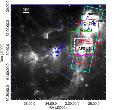
Figure 1.— WISE 22 $\mu$m wide field image ($\sim$ 2^∘$\times$2^∘) covering W4 super bubble centred at the cluster IC 1805, along with W3 GMC at its west. Locations of the important sub-regions of the W3 complex are marked and the boxes represent the area covered for various observations (green: NEWFIRM; red: IRAC; cyan: MIPS). Magenta box shows the area ($\sim$ 24^′ $\times$ 24^′) corresponding to AFGL333 region, based on the low resolution ¹²CO(J=3-2) map by Sakai et al. (2006) and the white dashed box represents the area considered in this study. The blue circles denote the locations of the probable massive members (earlier than B3V) in the complex obtained from SIMBAD database.

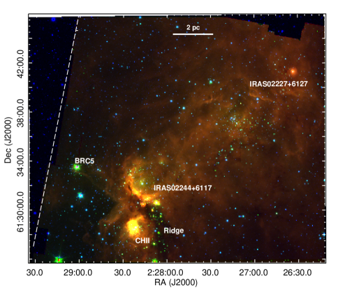
Figure 2.— Color composite image of $\sim$ 24^′$\times$20^′ area considered in this study (centered at $\alpha_{2000}$ = $02^{h}27^{m}48^{s}$; $\delta_{2000}$ = $+61^{\circ}35^{\prime}58^{\prime\prime}$) made using 2.1 $\mu$m (blue); 4.5 $\mu$m (green) and 8.0 $\mu$m (red) images. The important sub-regions are marked and the area to the left of dashed line is not covered by 4.5 and 24 $\mu$m bands.

2. Observations and point source catalogs

2.1. NEWFIRM-NIR imaging and photometry

We obtained NIR observations of AFGL333 in $JHK_{s}$ bands using the National Optical Astronomical Observatory (NOAO) Extremely Wide Field InfraRed Imager (NEWFIRM; Probst et al. 2004) camera on the 4m Mayal telescope at Kitt Peak National Observatory (KPNO) on 06 December 2009. The NEWFIRM camera contains 4 InSb 2048$\times$2048 pixel arrays arranged in a 2$\times$2 pattern with a field of view of 28^′$\times$28^′ (16.2 $\times$ 16.2 pc² at d= 2kpc) and a pixel scale of 0.4^′′ (0.0039 pc) per pixel. The area coverage of this observation is shown by a green box in Fig. 1. We took 50, 48 and 72 second exposures for $J,H$ and $K_{s}$ bands, respectively at 9 dithered positions. The dither offsets were large enough to fill in the 1^′ gap between CCDs. During our observations, the seeing was around $\sim$ 1^′′.0 - 1^′′.2. Standard processing of dark frame subtraction, flat fielding, sky-subtraction and bad pixel masking was performed by the NEWFIRM Science Pipeline (Swaters et al., 2009) and final stacked images were produced in each band.

We used the DAOFIND task in IRAF to extract the preliminary list of point sources in the $K$-band image. This algorithm provides additional statistics of the point sources such as roundness, sharpness etc. In order to avoid the artifacts and false detections, we selected only those sources having S/N $>$ 5. Following Stetson (1987), we set the roundness limits as -1 to +1 and sharpness limits as 0.2 to +1, which should eliminate the bad pixel brightness enhancements and the extended sources such as background galaxies from the point source catalogue. Due to the non-uniform background nebular emission as well as crowdness of the field, some sources were missed in the automatic detection algorithm. Such sources were manually identified and added in the final source list if they satisfy the above S/N, roundness and sharpness criteria. The list was again visually checked for any spurious source detection and were deleted from the list. The astrometry has been corrected with respect to the 2MASS point source catalog and the astrometry accuracy of our final source list is $\sim$ 0^′′.3

The final source list was fed into the DAOPHOT’s ALLSTAR routine to obtain the point spread function (PSF) photometry in $J$, $H$ and $K_{s}$ bands. Absolute photometric calibration was obtained using the Two Micron All Sky Survey (2MASS) data (Skrutskie et al., 2006), with quality flag better than ’A’ in all the three bands. We matched up bright isolated stars from our NEWFIRM catalogs with sources from 2MASS within a radius of 1^′′.0 and obtained zero points. The rms scatter between the calibrated NEWFIRM and 2MASS data (i.e., 2MASS-NEWFIRM data) for the $J$, $H$, and $K_{s}$ bands were 0.06, 0.06 and 0.07 mag, respectively. The saturated point sources in the NEWFIRM catalog were replaced by 2MASS magnitudes. We finally created the $JHK_{s}$ photometry catalog by spatially matching the detected sources in three bands within a match radius of 1^′′.0. Only those sources satisfy our reliability criteria in all three bands (i.e., photometry uncertainty $<$0.2 mag) were included in the final list. The total number of sources detected in each band and the detection limits are listed in Table 1. Compared to the 2MASS completeness limits in $JHK_{S}$ bands (i.e., 15.9, 15.1 and 14.3 mag), the new photometry is deeper by 4.6, 3.6 and 3.7 mag in $J$, $H$ and $K_{s}$ bands, respectively and thus adding 10444, 10624 and 11441 more sources than the existing 2MASS catalog.

2.2. Spitzer-IRAC-MIPS imaging and photometry

Images from the Spitzer space telescope (Werner et al., 2004) using Infrared Array Camera (IRAC, Fazio et al. 2004) centered at 3.6, 4.5, 5.8 and 8.0 $\mu$m (ch1, ch2, ch3 and ch4) were obtained from the Spitzer archive. These observations were taken on 10 January 2004 and 19 February 2007 (Program IDs: 30955, 127; PIs: R. Gehrz, T. Moore) in high dynamic range (HDR) mode with three dithers per map position and two images each with integration time of 0.4 s and 10.4 s per dither. Preliminary analyses of these data sets have been presented in Ruch et al. (2007) and Rivera-Ingraham et al. (2011). The total area coverage by these two observations is $\sim$ 28^′ $\times$ 63^′ ($\sim$ 16 $\times$ 37 pc²; see Fig. 1).

We obtained the cBCD (corrected basic calibrated data) images (version S18.7.0) from the archive and the raw data was processed and calibrated with IRAC pipeline. The final mosaic images were created using the MOPEX pipeline (version 18.0.1) with an image scale of 1^′′.2 per pixel. In order to avoid the saturation due to bright nebular emission, we processed the long and short exposure frames seperately. We kept the settings similar to the NEWFIRM data (see Section 2.1) to make a preliminary source list using DAOFIND in IRAF. Since the IRAC bands suffered from variable background nebular emission over small spatial scales, single point source detection threshold across the entire mosaic image does not detect all the potential point soucres in the field. We used various detection threshold values over multiple iteration to enable the detection of all faint sources in the field. The reliability of the sources were decided based on their S/N, roundness and sharpness values. Many spurious sources in the nebulosity were identified by visual inspection and deleted from the automated detection list.

To extract the flux of the point sources, we performed point response function (PRF) fitting on IRAC images in multi frame mode, using the tool Astronomical Point Source EXtraction (APEX), developed by the Spitzer Science Centre (see Jose et al. 2013 for details). Flux densities were converted in to magnitudes using the zero-points 280.9, 179.7, 115.0 and 64.1 Jys in the 3.6, 4.5, 5.8 and 8.0 $\mu$m bands, respectively, following the IRAC Data Handbook. The saturated bright sources in the long integrated images were replaced by the sources from short exposure images. To ensure optimal photometry, only those sources with S/N $>$ 5 and photometry uncertainty $<$0.2 mag in individual bands are considered for further analysis. The number of sources detected in each band and the detection limits are given in Table 1. The IRAC data of the four band passes were merged by matching the coordinates using a radial matching tolerance of 1^′′.2. Thus our final IRAC catalog contains photometry of 29224 sources that are detected in one or more IRAC bands, including 1567 sources detected in all four IRAC bands.

AFGL333 was observed in 24 $\mu$m using the Multi band Imaging Photometer for Spitzer (MIPS; Rieke et al. 2004) on 03 February 2004 (Program ID: 127, PI: R. Gehrz). The observations covers an area $\sim$ 26^′ $\times$ 89^′ ($\sim$ 15 $\times$ 52 pc², see Fig. 1). We obtained the BCD images (S18.13.0) from the Spitzer archive and the final mosaics were created using the MOPEX pipeline (version 18.0.1) with an image scale of 2^′′.45 per pixel. We applied the same source detection technique and reliability criteria as described for IRAC to the MIPS 24 $\mu$m image. To extract the flux, we performed the PRF fitting method in the single frame mode. The zero-point value of 7.14 Jy from the MIPS Data Handbook has been used to convert flux densities to magnitudes. The final catalogue contains the 24 $\mu$m photometry of 327 sources having uncertainty $<$ 0.2 mag.

2.3. Completeness limits

Figure 3.— Source histograms for bands $J$ through 24 $\mu$m showing the limiting magnitude and completeness limit for each band. The vertical lines indicate the adopted completeness limit.

In order to analyze the photometric incompleteness, the artificial star experiment has been performed using the ADDSTAR routine in IRAF on the $K_{s}$-band image (see Jose et al. 2012 for details). Briefly, artificial stars were added at randomly generated positions to the $K_{s}$-band image. The luminosity distribution of artificial stars was chosen in such a way that more number of stars were inserted towards the fainter magnitude bins. The frames were reduced using the same procedure used for the original frames (Section 2.1). The ratio of the number of stars recovered to those added in each magnitude interval gives the completeness factor as a function of magnitude. The faintest magnitude bin, where the fraction of sources recovered was greater than 90% was adopted as the completeness limit. We thus obtained $\sim$ 90% completeness of the data for the magnitude limit of 17 in $K_{s}$-band. The completeness limits of individual bands were also analyzed using the histogram distributions of the measured source magnitudes (see Fig. 3; Table 1). The turnover point in source count curves can serve as a proxy to show the completeness limit (e.g., Jose et al. 2013; Willis et al. 2013; Samal et al. 2015). The photometric completeness obtained from histogram analysis is consistent with that estimated from the artificial star experiment in $K_{s}$-band.

Table 1Point source catalog summary for various bands

Band	Sources in	within	detection	90% completeness
	total areaa	AFGL333b	limit (mag)	limit (mag)
$J$	13162	7194	20.5	18.0
$H$	13472	7447	18.7	17.5
$K_{s}$	13573	7525	18.0	17.0
ch1	22361	5346	17.8	16.0
ch2	20502	6095	17.5	16.0
ch3	4452	1408	15.3	13.0
ch4	2400	799	14.0	12.0
$[24]$	327	134	9.3	7.0

^a Number of sources within the field of view of individual bands.
^b Number of sources within AFGL333 area considered in this study.

2.4. Final point source catalog

We created the final photometry catalog by spatially matching and merging the detected sources in various bands. A search for the IRAC counterparts of the NIR sources within a match radius of $1^{\prime\prime}$.2 identified 7168 sources at least in one of the IRAC bands. Of the 327 detection in MIPS band, within a match radius of 2^′′.5, 304 sources have IRAC counterparts at least in one band and 135 sources with NIR counterparts.

We compared our IRAC and MIPS photometry with the existing catalogs in the literature (Ruch et al. 2007; Rivera-Ingraham et al. 2011). The root mean square (rms) scatter between the photometry from this work and that of Rivera-Ingraham et al. (2011) are found to be within 0.1 mag and are within 0.2 mag with Ruch et al. (2007) for all IRAC bands. This dispersion occurs mainly due to the different techniques adopted for the flux estimation, however is within the uncertainty limit in this study. The rms scatter between the MIPS-24$\mu$m photometry of this study with that of Ruch et al. (2007) and Rivera-Ingraham et al. (2011) is $\sim$ 0.5 mag.

Table 1 lists the number of sources detected in each band as well as their detection and completeness limits. The number of sources in each band is different due to respective sensitivity limits and area coverage (see Fig. 1). The AFGL333 region is projected on the sky over an area $\sim$ 24^′ $\times$ 24^′ (see Fig. 1; $\sim$ 193 pc²), based on CO emission maps from Sakai et al. (2006) and Bieging & Peters (2011). However, the coverage area of the near-IR, IRAC, and MIPS observations are all different and do not cover the entire region (see Fig. 1). An area ( $\sim$ 24^′$\times$20^′, 161 pc²) covered by most of the wavelengths is considered for this analysis (see Fig. 2 and white box in Fig. 1). Our coverage area for extinction maps (Section 3) and our YSO identification (Section 4) miss $\sim$ 15% of AFGL333 area to its south compared to the area delineated by Sakai et al. (2006). The number of sources detected within the area of interest in each band is given in column 3 of Table 1.

3. Mapping the dust and gas in AFGL333

The main goal of this study is to obtain the census of young stellar objects as a tool to understand the cloud structure and star formation activity within AFGL333 region. The census of young stellar objects based on color-color cuts requires a quantification of how color-color selections are affected by extinction. In this section, we map the structure of gas and dust in the AFGL333 molecular cloud. These extinction maps also allow us to identify the sites of active star formation.

The primary dust map used in this paper is a map of extinction calculated from near-IR colors of background stars (Section 3.1). In Section 3.2, we create a map of molecular gas from 1.3 mm CO emission. In Section 3.3, the near-IR extinction map is then compared to the CO map and a published dust column density map calculated from emission in Herschel imaging, to confirm consistency within uncertainties between the three methods.

3.1. Near-IR extinction maps of AFGL333

The dust column density may be mapped by calculating the extinction to background sources. Our extinction map is calculated by dereddening the $H-K_{s}$ of background stars to the nominal average intrinsic $H-K_{s}$ of field stars. i.e., $A_{K}$=1.82 $\times$ $(H-K_{s})_{obs}-(H-K_{s})_{int}$, where, $(H-K_{s})_{int}$=0.2 is considered as the average intrinsic color of field stars (Allen et al. 2008; Gutermuth et al. 2009; Jose et al. 2013).

Since AFGL333 is situated at a distance of $\sim$ 2.0 kpc, an average foreground extinction of $A_{V}$= 2.6 mag is expected (0.15 mag kpc^-1 in $K_{s}$ band, Indebetouw et al. 2005; Chavarría et al. 2008; $A_{K}$/$A_{V}$ = 0.114; Cardelli et al. 1989). This value is consistent with the minimum interstellar reddening obtained towards W3 by Oey et al. (2005) and also with the all-sky dust map based on PAN-STARRS and 2MASS photometry by Green et al. (2015). Thus in order to eliminate the foreground contribution, only those stars with $A_{V}$ $>$ 2.6 mag are used for getting the extinction map. To generate the extinction map, the method described by Gutermuth et al. (2005) is followed. Briefly, the region is divided into uniform grids and the mean and standard deviation of $A_{V}$ values of N nearest neighbour stars from the center of each grid was measured. The algorithm rejects any stars with $A_{V}$ values $>3\sigma$ from the mean. The outlier rejection in this application should primarily remove the young stellar objects with IR excess, where $H-K_{s}$ excess mainly arising from their circumstellar disk (Meyer et al., 1997). The resulting $A_{V}$ map is convolved with a Gaussian kernel to get the final mean value. The final extinction map is generated with N=6 and angular resolution of $20^{\prime\prime}$ (Fig. 4), after several iteration to achieve a good compromise between resolution and noise (Gutermuth et al., 2009).

The average value of $A_{V}$ across AFGL333 is found to be $\sim$ 10 mag. The extinction map of AFGL333 given in Fig. 4 shows two distinct features: a cavity with low extinction ($A_{V}$ $<$3.5 mag) towards the eastern side of the image and a highly extincted western half. A comparison with the sub-mm and C¹⁸O(J=1-0) observations (see Moore et al. 2007; Sakai et al. 2006) shows that the highest extinction areas coincide with the dense molecular cores detected towards AFGL333, including the curved features of BRC 5 and AFGL333 Ridge.

The uncertainty in the extinction measurement is dominated by the systematic error in the adopted extinction law, assumed here to be based on a total-to-selective extinction $R_{V}=3.1$ typical of the diffuse interstellar medium. However, dense clouds usually have $R_{V}$ values $>$ 4-5.5, especially at $A_{V}>20$ mag (Mathis 1990; Chapman et al. 2009), which would lead to a $\sim 20\%$ overestimate in the extinction (for $R_{V}$ = 5.5, $A_{K}$/$A_{V}$ = 0.134; Cardelli et al. 1989). Only the molecular ridge, which totals $<$ 10% of the total cloud area, has $A_{V}$ $>$ 20 mag.

Extinction estimates from stellar colors should be calculated using only background sources. However, the diskless members of AFGL333 cannot be distinguished from background stars, and their inclusion in our analysis may lead to underestimating the extinction. Based on our extinction-corrected comparison of AFGL333 to nearby control field (see Section 4.3), the diskless members of AFGL333 are $\sim$ 30% of the stars considered here as background sources in regions with $A_{V}=10$ mag ($\sim$ 45% for $A_{V}=20$ mag). The inclusion of diskless stars therefore moderately underestimates the extinction throughout the cloud, and is again especially severe in high extinction regions along the molecular ridge.

A smaller uncertainty is introduced by our spectral type sensitivity of background stars. The 90% completeness limit in the $K_{s}$-band is 17 mag (see Section 2.3), which corresponds to background stars at 2 kpc of K7 for $A_{V}=0$ mag, K4 for 10 mag, and G4 for 20 mag. These differences will lead to an uncertainty of $\sim 2$ mag in $A_{V}$, with the ridge again most affected.

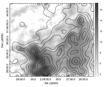
Figure 4.— The grey scale represents the $V$-band extinction map made from the CO column density map and the contours are the $V$-band extinction map generated from the $(H-K_{s})$ colors by nearest neighbourhood method assuming $R_{V}$= 3.1. The contours begin at $A_{V}$=4 mag and increase by 1.5 mag till a maximum of 25 mag.

3.2. Extinction map from the CO column density

We used the ¹²CO (J=2-1) and ¹³CO (J=2-1) position-velocity data cubes for the entire W3 region from Bieging & Peters (2011) to derive a gas column density map of the area around AFGL333. The emission of these two CO isotopologues was analyzed with a non-LTE statistical equilibrium model grid and a large velocity gradient radiative transfer code (see Kulesa et al. 2005) to find the CO total column density at each map pixel. The model incorporates gas heating dominated by photons via the photoelectric effect together with the observed CO line intensity, to estimate the UV radiation incident at each point in the map. The CO abundance and total hydrogen column density ($N(H)$ = $N(HI)$ $+$ $2N$ (H₂)) are calculated following the photodissociation models of Black & van Dishoeck (1987) and van Dishoeck & Black (1988). The visual extinction $A_{V}$, is found using the ratio $N(H)/A_{V}=1.8\times 10^{21}$ cm^-2mag^-1 (Bohlin et al., 1978).

Figure 4 shows the results of this calculation, plotting the CO-derived visual extinction ($A_{V}$) in grayscale and the $K$-band extinction from the NIR point source catalog as contours. The CO-derived column density maps are subject to systematic uncertainties in the assumed values for the ¹²CO/¹³CO isotopic abundance ratio and the CO/H₂ molecular abundance ratio. For the galacto-centric radius of AFGL333, we assume a ¹²CO/¹³CO isotopic ratio of 80 with a probable uncertainty of $\sim$ 30% (e.g., Milam et al. 2005). We assume a CO/H₂ abundance of $10^{-4}$ also with an uncertainty of $\sim$ 30%. The observed CO lines become saturated for the highest extinction regions ($A_{V}\geq 20$ mag), and CO may become depleted onto grains at high density and low temperature. Column densities may therefore be underestimated, but this effect should be limited to a small fraction of the total area of the region.

3.3. Comparing extinction maps

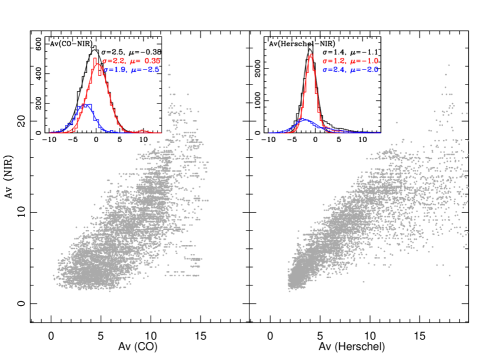
Figure 5.— Comparison of $A_{V}$ measured from near-IR data with CO derived column density (left) and with dust column density map calculated from Herschel far-IR imaging by Rivera-Ingraham et al. (2013) (right). The mean and rms of the gaussian fit to the scattering is shown in the inset plot, where black indicates for all values of $A_{V}$, red is for $A_{V}$ $<$ 10 mag and blue is for $A_{V}$ $>$ 10 mag, respectively.

Figure 4 provides qualitative support for the general cloud structure, as calculated from the near-IR extinction and CO column density. These results are also qualitatively consistent with the dust column density map calculated from Herschel far-IR imaging by Rivera-Ingraham et al. (2013). However, each of these methods suffers from biases and uncertainties (e.g. Pineda et al., 2010), all of which are difficult to independently evaluate. In this subsection, we compare results from different methods to measure extinction to quantify empirical uncertainties in the extinction map.

Figure 5 compares the average near-IR extinctions to extinctions estimated from CO column density and Herschel dust column density maps within grids of size 38^′′. Below $A_{V}=10$ mag, the three sets of extinctions are well correlated. The extinctions from CO column density are 0.35 mag in $A_{V}$ smaller than those from near-IR colors, but with a large scatter of rms$=2.2$ mag between the two values. The extinctions from the far-IR dust column densities are much more tightly correlated with the near-IR extinctions, with an rms of 1.2 mag., but are $1$ mag smaller than the near-IR extinction. At $A_{V}>10$ mag, these correlations become much worse. The near-IR colors overestimates high extinctions by $2-2.5$ mag, with a scatter of $2-2.5$ mag that is caused by a tail of very high extinction that is undetected in the near-IR.

The tight correlation between the dust emission and near-IR extinction indicates random uncertainties of $\sim 1$ mag in regions of low-modest extinction. The absolute comparisons for both the dust emission and the near-IR extinction depend sensitively on correction for foreground and background dust. The CO column density map should be robust to these uncertainties, and establishes that systematic uncertainties are $\sim 0.35$ mag. The near-IR extinction map becomes much more unreliable when $A_{V}>10$ mag, as expected from our description of uncertainties in this method in Section 3.1. However, at high column densities, these comparisons are sensitive to the filling factor of dense gas and dust within the $38^{\prime\prime}$ boxes. If the dense material is concentrated in small regions, the near-IR extinction map may be a better estimate of the median extinction in a region. The near-IR extinction map has no sensitivity to these optically thick regions, since few background stars are detectable.

These comparisons establish that the near-IR extinction map therefore provides a reasonable estimate of the extinction to most stars in AFGL333 at low extinction. This map will be adopted for the remainder of the paper. The extinction map and our stellar census is unreliable in the densest regions, which occur mainly along the AFGL333 Ridge.

4. Census of young stellar objects in AFGL333

Several classification schemes have been developed in recent years to differentiate between YSOs with dominant envelope emission, circumstellar disk emission and diskless sources. YSOs are often categorized into Class 0, I, II or III evolutionary stages (Lada & Wilking, 1984). Class 0 objects are deeply embedded protostars experiencing cloud collapse and are extremely faint at wavelengths shorter than 10 $\mu$m. Class I YSOs are infrared bright with the emission dominated by their spherical envelope. With only near-IR and mid-IR data it is impossible to distinguish Class 0 from Class I objects. Hereafter these objects are grouped together and called Class I in this study. A Class II YSO has no envelope and is characterised by the presence of an optically thick, primordial circumstellar disk, which gives excess emission in IR. When the circumstellar disk becomes optically thin, the star is classified as Class III.

In this section, we identify and classify Class I and Class II sources using the 1 - 24 $\mu$m SEDs. We do not classify the diskless Class III YSOs because they are indistinguishable from the field stars in their IR colors (see Section 5.2 for details). In the first step, we use those sources detected in all four IRAC bands to classify the objects as Class I / Class II based on their color excesses. Selection of YSOs based on the four IRAC band colors may not be complete, as we are likely to have missed many sources that fall in the region with bright nebulosity in [5.8] and [8.0] $\mu$m bands as well as due to the limited sensitivity of these two bands (see Table 1). In order to account for the missing YSOs in [5.8] and [8.0] $\mu$m bands, we identify more YSOs based on their color excess in $H$, $K_{s}$, $[3.6]$ and $[4.5]$ $\mu$m. Finally, we re-examine the entire catalog of sources having 24 $\mu$m photometry and more YSOs are added to the list based on the color excess of 24 $\mu$m in combination with any IRAC bands. Possible contaminants are also discussed. Estimating the total population of AFGL333 members requires identifying the diskless Class III population. Since we cannot discriminate between foreground and background stars, this estimate relies on statistical estimates of the foreground and background populations from a nearby control region. We consider a control field region from our near-IR images centered at $\alpha_{2000}$ = $02^{h}28^{m}28^{s}$; $\delta_{2000}$ = $+61^{\circ}42^{\prime}45^{\prime\prime}$, $\sim$ 10^′ north of BRC 5. This region is devoid of nebulosity in $K_{s}$ band. The column density map from dust emission by Rivera-Ingraham et al. (2013) shows that the region suffers from normal interstellar reddening. Therefore we consider this a safe region to be used as a control field region.

4.1. Selection of YSOs using IRAC data

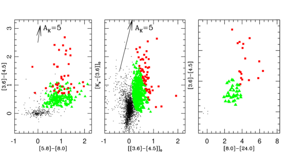
Figure 6.— Color-color diagrams of all the sources (black dots) identified within AFGL333. The YSOs classified as Class I and Class II based on the color criteria by Gutermuth et al. (2009) are shown using red rectangles and green triangles, respectively. The reddening vector for $A_{K}$ = 5 mag is plotted using the reddening law from Flaherty et al. (2007). left: [3.6]-[4.5] vs [5.8]-[8.0] color-color diagram of all the IRAC sources, middle: dereddened $[K_{s}-[3.6]]_{0}$ vs $[[3.6]-[4.5]]_{0}$ color-color diagram for all the IRAC sources having NIR counterparts. right: [3.6]-[4.5] vs [8.0]-[24.0] color-color diagram of all the IRAC sources with counterparts in 24$\mu$m.

In order to classify the YSOs detected in all IRAC bands into Class I and Class II, we adopt the color criteria given by Gutermuth et al. (2009). Of the 1567 sources detected in all the IRAC bands (see Section 2.2), 538 sources are within the AFGL333 area considered for this study. Of these, 40 have colors consistent with Class I and 188 have colors consistent with Class II, respectively. However, in rare cases, highly reddened Class II sources could have the colors of a Class I source. In the highly reddened regions (i.e., the ridge), the average $A_{V}$ $\sim$ 20 mag can cause a shift of $\sim$ 0.18 mag in the [3.6]-[4.5] color of a star (Flaherty et al., 2007). If the color excess of Class II YSOs are shifted due to the presence of reddening up to $A_{V}$ $\sim$ 20 mag, $\sim$ 20% of Class I YSOs are expected to be misclassified Class II sources. In Fig. 6 (left panel), the [3.6]-[4.5] vs [5.8]-[8.0] color-color diagram is shown, where the Class I and Class II sources are shown in red and green colors, respectively.

4.2. YSOs from $H,K_{s},[3.6]$ and $[4.5]$ $\mu$m data

Additional YSOs are identified based on their color excess in $H$, $K_{s}$, 3.6 and 4.5 $\mu$m bands. We dereddened the individual point sources based on their location on the extinction map (see Fig. 4) using the extinction law by Flaherty et al. (2007). We followed the various color criteria by Gutermuth et al. (2009) to classify the YSOs in the Class I and Class II category. After removing the YSOs which are already identified in Section 4.1, a total of 434 more sources are added to the YSO list. Of these, 30 and 404 sources have colors consistent with Class I and Class II, respectively. However, the intrinsic uncertainty of $\sim$ 2 mag in $A_{V}$ measurement (see Section 3) can cause a variation in the number of Class I sources by $\sim$ 20 % and Class II sources by $\sim$ 7%. Fig. 6 (middle panel) shows the dereddened $K_{s}$-[3.6] vs [3.6]-[4.5] color-color diagram, where Class I and Class II sources are shown in red and green colors, respectively.

4.3. Additional YSOs from $H$, $K_{s}$ and [4.5] $\mu$m data

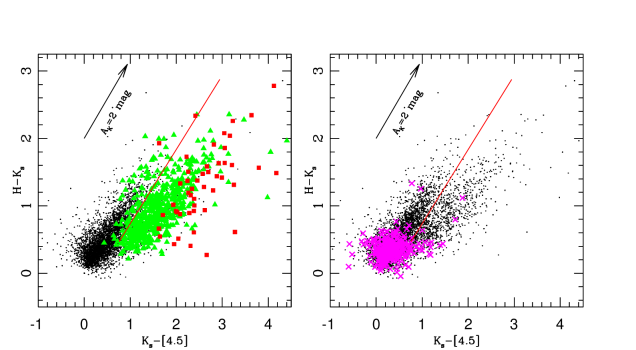
Figure 7.— left: $K_{s}-[4.5]$ vs $H-K_{s}$ color-color distribution of all the sources (black dots) within AFGL333 along with the Class I (red rectangles) and Class II (green triangles) YSOs identified. Red straight line represents the reddening vector drawn from the tip of the dwarf locus (Patten et al., 2006) using the reddening law from Flaherty et al. (2007). right: Same as in left panel. Magenta sources represent the distribution of sources in the nearby control field.

We used a combination of $H,K_{s}$ and 4.5 $\mu$m bands to identify the additional YSOs within AFGL333 (Samal et al., 2014). Among all the IRAC bands, the 4.5 $\mu$m band not only provides the largest number of point source detections, but also has advantage of being unaffected by polycyclic aromatic hydrocarbons (PAHs). Three other IRAC bands are contaminated by PAHs (Whitney et al. 2008; Povich et al. 2013). Fig. 7 (left panel) shows the $K_{s}-[4.5]$ vs $H-K_{s}$ color-color distribution of all sources detected within AFGL333 along with the candidate YSOs identified in the previous sections. The reddening vector from the tip of the dwarf locus (Patten et al., 2006) is also shown.

Fig. 7 (right panel) shows the color-color distribution of sources in the nearby control field region (see setcion 2.4), which should have the distribution of non-YSO sources in the same Galactic direction as that of AFGL333. A comparison of the distribution of YSOs already identified in the previous sections (Fig. 7, left panel) and control field region shows that all the sources that are located towards the right side of the reddening vector are likely to have NIR excess. After excluding the YSOs that are already identified, several more sources are located towards the right side of the reddening vector. Those sources with $H-K_{s}>$ 0.65 mag and with an excess $>$ 3$\sigma$ (where $\sigma$ is the average uncertainty in color) from the reddening vector (see Fig. 7) are considered as YSOs. Thus a total of 121 more sources are added to the YSO list. In order to confirm these sources as YSOs, we checked their location on the $H-K_{s}$ vs $K_{s}$ - [3.6] diagram and all the sources except four, which have 3.6 $\mu$m detection, are found to be located towards right side of the reddening vector. These sources also satisfy the color-color criteria to identify YSOs using $J$, $H$ and 4.5 $\mu$m data given by Zeidler et al. (2016) (i.e., $K_{s}$-[4.5] $>$ 0.49 mag and $J-H$ $>$ 0.7 mag). Also, $\sim$ 70% of these sources satisfy the color and magnitude selection scheme implemented by Rivera-Ingraham et al. (2011) using $J,H,K_{s}$ data.

By selecting only those objects towards the right side of the reddening vector and by applying an additional color cut at $H-K_{s}>$ 0.65, we reduce the number of contaminating background objects that are reddened by the clouds. A few YSOs may be missing in this approach, but the selected sources are more reliable candidates with NIR excess (Samal et al. 2014; Zeidler et al. 2016). Since most of these newly identified NIR excess sources fall in the regime of the already identified Class II YSOs, we include them in the Class II category.

4.4. YSOs using 24 $\mu$m excess

In the final step, the entire catalog of sources with 24 $\mu$m photometry is re-examined. Any source that lacks a detection in some IRAC bands but has bright 24 $\mu$m photometry (i.e., [24]$<$ 7 mag; [X]–[24] $>$ 4.5; where [X] is any IRAC band) is likely to be a deeply embedded protostar (Gutermuth et al., 2009). Using this criteria, we identify 29 new Class I sources. All previously identified Class I YSOs with MIPS detections have colors [5.8]–[24] $>$ 4 or [4.5]–[24] $>$ 4 that confirm their classification. The right panel of Fig. 6 shows the [3.6]-[4.5] vs [8.0]-[24] color-color diagram of all the IRAC sources having counterparts in 24 $\mu$m. The candidate Class I and Class II sources are marked in red squares and green triangles, respectively.

4.5. Final catalog of YSOs

Our NIR and MIR color criteria using MIPS, IRAC and NEWFIRM photometry identifies 812 candidate YSOs (99 Class Is and 713 Class IIs) associated with the AFGL333. Table 2 summarizes the statistics of YSOs in various bands. Sample entries of photometric data of all the stars within AFGL333 is given in Table 3 and the full version is available in electronic format.

The latest census of YSOs (Class I and Class II) in AFGL333 by Rivera-Ingraham et al. (2011) identified 156 YSOs within the area considered in this study. Of these, 138 are recovered in our YSO list (37 Class I, 101 Class II). The slight discrepancy in the number of YSOs is due to the different YSO selection criteria adopted in these two studies. Of the 37 Class I sources in our list, 31 are classified as Class 0/I and 6 as Class II in Rivera-Ingraham et al. (2011). Of the 101 Class II sources in our list, 91 are classified as Class II and 10 as class I in their list. They have also identified an additional 83 candidate pre-main sequence sources in the region using a 2MASS based color-color and magnitude selection scheme. Of these, 70 are recovered in our YSO list (3 Class I, 67 Class II). Their survey was limited by the sensitivity of 2MASS data. In conclusion, the previous survey of this region identified 239 candidate YSOs and due to the improved sensitivity of $JHK_{s}$ data in this study by $>$ 3 mag in each bands, we have identified 573 more YSOs within AFGL333.

Table 2YSO catalog summary in various bands

Band	Class I	Class II
IRAC	40	188
$H,K_{s},3.6,4.5$	30	404
$[24]+$IRAC(any)	29	$-$
$H,K_{s},4.5$	$-$	121
total	99	713

Table 3Photometric data^a of all point sources within AFGL333.

$\alpha_{(2000)}$	$\delta_{(2000)}$	$J$	$H$	$K_{s}$	$[3.6]$	$[4.5]$	$[5.8]$	$[8.0]$	$[24]$	Class
deg	deg	mag	mag	mag	mag	mag	mag	mag	mag
36.9357	+61.6750	12.10	11.41	10.88	9.98	9.74	9.38	9.13	-	Class II
36.6905	+61.6978	12.16	11.49	10.93	9.53	9.19	8.40	7.64	5.18	Class II
37.1812	+61.4949	12.32	11.40	10.80	10.26	9.60	8.91	7.54	4.15	Class II
36.6395	+61.6879	12.68	11.96	11.53	11.13	10.74	-	-	-	Class II
37.1809	+61.5262	12.81	12.28	11.88	11.21	10.90	10.72	10.53	-	Class II
36.7891	+61.9122	12.87	12.14	11.72	11.23	10.96	10.67	10.31	-	Class II
36.8007	+61.6182	12.94	11.51	10.49	9.38	8.90	8.49	7.53	4.60	Class II
36.7908	+61.4332	14.92	14.18	13.66	13.19	13.13	12.68	11.54	-	Class III/field stars

^a The complete table is available in electronic form.

4.6. Source contamination rate

Our candidate YSO population may be contaminated by the background sources including PAH-emitting galaxies, broad-line AGNs, unresolved knots of shock emission, PAH-emission contaminated apertures etc., that mimic the colors of YSOs. Since we are observing through the Galactic plane, contamination due to galaxies should be negligible (Massi et al., 2015). In order to have a statistical estimate of possible galaxy contamination in our YSO sample, we used the Spitzer Wide-area Infrared Extragalactic (SWIRE) catalog coming from the observations of the ELAIS N1 field (Rowan-Robinson et al., 2013). SWIRE is a survey of the extragalactic field using Spitzer-IRAC and MIPS bands and can be used to predict the number of galaxies with colors that overlap with YSO colors (Evans et al., 2009). The SWIRE catalog is resampled for the spatial extent as well as the sensitivity limits of our observations in AFGL333 and is also reddened by the average reddening of AFGL333 (i.e. $A_{V}$ = 10 mag, see Section 3). The YSO selection criteria is applied to the resampled SWIRE catalog and only $\sim$ 2% of our YSO sample found to be compatible with the galaxy colors. Similarly, using the color criteria given by Robitaille et al. (2008), $\sim$ 2% of YSOs seem to have colors consistent with AGB stars.

Finally, a comparison between the distribution of control field stars and the YSOs (see Fig. 7) shows that $<$ 5% of YSOs coincide with the location of field stars. In summary, the contribution of various contaminants in our YSO sample is $<$ 5 % (i.e., galaxies $\sim$ 2%, AGBs $\sim$ 2%), which is a small fraction of the total number of YSOs.

We also applied the Gutermuth et al. (2009) color-color criteria to the candidate YSOs identified within AFGL333. $\sim$ 38% of Class I and $\sim$ 15% of Class II of the final YSO list in Table 2 are matched with the colors of PAH contaminated apertures, shock emissions, PAH emitting galaxies and AGNs. The major contribution is from the contamination by AGNs. However, several studies (e.g., Koenig et al. 2008; Rivera-Ingraham et al. 2011; Willis et al. 2013) have noticed that the use of Gutermuth et al. (2009) criteria for a region at $\sim$ 2kpc would likely provides an overestimation of the contamination.

4.7. Mass completeness limit of YSOs

The $J$ vs $(J-H)$ and $H$ vs $(H-K_{s})$ color-magnitude diagrams (Fig. 8) are used to get an estimate of the mass range of the candidate YSOs identified within AFGL333. The Class I and Class II YSOs identified from various color combinations of IRAC and NIR bands in Section 4 are shown using red rectangles and green triangles, respectively in Fig. 8. The pre-main sequence isochrone with age 2 Myr (Bressan et al., 2012) and reddening vectors for several masses are also shown. The wide variation in the colors of YSOs in Fig. 8 is caused by variable extinction and different evolutionary stages of sources within AFGL333. In general, the majority of YSOs lie in the mass range $\sim$ 0.1 - 2 $M_{\odot}$.

The mass completeness limit for our YSO survey is dictated by the photometric completeness and wide range of YSO colors. We selected the YSO sample based on the IRAC, $HK_{s}$+IRAC and IRAC+MIPS color combinations (see Section 4). Within AFGL333, 85% of the Class I sources have counterparts in IRAC 4.5 $\mu$m band and all the Class II sources are detected in 4.5 $\mu$m (see Table 2). The 90% photometry completeness limits of $K$ and 4.5 $\mu$m-bands are estimated to be $\sim$ 17 and 16 mag, respectively (see Section 2.3). Assuming a distance of 2.0 kpc for AFGL333 and average extinction $A_{V}$ as $\sim$ 10 mag (see Section 3), the photometric completeness limits in these bands correspond to an approximate stellar mass of $\sim$ 0.2 M_⊙ for a YSO of age $\sim$ 2 Myr (using the evolutionary tracks of Bressan et al. 2012). The completeness limit is $>$ 0.4 M_⊙ at high extinction regions such as the AFGL333 Ridge, where the extinction $A_{V}$ $>$ 20 mag. However, only $<$ 10% of the total area suffers this high extinction. Also, due to the IR excess, the YSOs will be brighter in IR bands compared to their main-sequence counterparts with only photospheric emission. So the completeness limits of Class I and Class II sources will be lower than 0.2 M_⊙, when compared to the diskless sources. The previous YSO survey of this region (Rivera-Ingraham et al., 2011) was limited by the 2MASS completeness limit, which corresponds to $>$ 1 M_⊙ for $A_{V}$ $\sim$ 10 mag. With the deep photometry, the current analysis probes the very low mass stars ($>$ 0.2 M_⊙) of the region. For further analysis, we include only those sources brighter than 16 mag in 4.5 $\mu$m.

Figure 8.— $J$ vs $(J-H)$ (left) and $H$ vs $(H-K_{s})$ (right) color-magnitude diagrams of all the sources (black dots) within AFGL333 region. The red rectangles and green triangles are the Class I and Class II YSOs identified in Section 4. Blue solid curve is the pre-main sequence isochrone of age 2Myr (Bressan et al., 2012) shifted for a distance of 2.0 kpc. The straight lines represent the reddening vectors for $A_{V}$= 20 mag that correspond to stellar masses of 0.2, 0.5 and 2 $M_{\odot}$.

5. Characteristics of young stellar objects, environment and star formation in AFGL333

In this section the final YSO catalog obtained from Section 4 is used to obtain their spatial distribution, mass distribution, stellar surface density and clustering properties.

5.1. Spatial distribution of YSOs and sub-clustering in AFGL333

The spatial distribution of YSOs can probe the fragmentation processes that lead to the formation of protostellar cores and the subsequent dynamical evolution of star forming regions. Fig. 9 shows the spatial distribution of the candidate YSOs (i.e., red: Class I; green: Class II;) overlaid on the 4.5 $\mu$m Spitzer image, where the YSOs are preferentially located in/around the regions of high extinction (see Fig. 4). The Class I YSOs follow the elongated nature of the molecular ridge seen in the CO maps of Sakai et al. (2006) and Bieging & Peters (2011) and in our extinction map shown in Fig. 4.

Since W3 is a complex star forming region, a high level of sub-clustering is expected and is evident in the spatial distribution of candidate YSOs (Fig. 9, left panel). In order to understand the level of sub-clustering within AFGL333, we generated the stellar density map using the nearest neighbourhood technique (Gutermuth et al., 2005). We followed the method introduced by Casertano & Hut (1985), where the stellar density $\sigma(i,j)$ inside a cell of a uniform grid with center at the coordinates $(i,j)$ is

$\sigma(i,j)$ = $N-1\over\pi r^{2}_{N}(i,j)$

where, $r_{N}$ is the distance from the center of the cell to the N^th nearest source. The value of N is allowed to vary depending on the smallest scale structures of the regions of interest. The surface density map for the candidate YSOs detected above the completeness limit is generated with a grid size of 10^′′ $\times$ 10^′′ and N=6 as a compromise between resolution and sensitivity of the map.

In the surface density map shown in the right panel of Fig. 9, three major groups of YSOs are identified, which agrees with our visual interpretation of the spatial distribution of YSOs. The main over-density corresponds to the group of YSOs associated with the AFGL333 Ridge and its surroundings, which itself appears to have multiple density peaks. Hereafter we name this group of YSOs as AFGL333-main. Within AFGL333-main, the YSO surface density peaks at the center of the cluster associated with the Hii region (i.e., IRAS 02245+6115; see Fig. 2). The second over-density of YSOs is located towards the north of AFGL333 Ridge, ($\alpha_{2000}$ = $02^{h}27^{m}14^{s}$; $\delta_{2000}$ = $+61^{\circ}36^{\prime}48^{\prime\prime}$) and the YSOs are associated with a mid-IR cavity seen in the background image. The majority of YSOs in this cluster are Class II sources. Hereafter we name this group of YSOs as AFGL333-NW1. One more cluster (AFG 333-NW2) is seen further north west of the region ($\alpha_{2000}$ = $02^{h}26^{m}34^{s}$; $\delta_{2000}$ = $+61^{\circ}41^{\prime}27^{\prime\prime}$) and $\sim$ 70 YSOs are associated with it.

Some of these groups of YSOs are part of known clusters in the literature. For example, the sub-group associated with BRC5, located at the outermost boundary of the HDL (IRAS 02252+6120) and with the Hii region (IRAS 02245+6115), host clusters (Bica et al., 2003). The latest clustering analysis of the W3 complex using minimum spanning tree method by Rivera-Ingraham et al. (2011) identified 8 stellar groups (IDs 0 to 7) as part of AFGL333. Of these, 5 groups (IDs 1, 3, 4, 6 and 7) are within the area considered in this study and others are outside the area. The groups 6 and 4 are associated with AFGL333-NW1 and groups 1, 3 and 7 belong to AFGL333-main. The individual stellar peaks in Fig. 9 coincide with that of the stellar groups identified by Rivera-Ingraham et al. (2011). Though the individual groups are assumed to be at various evolutionary stages and at different environments (see Rivera-Ingraham et al. 2011 for details), due to our limited spatial resolution and detection sensitivity in this study we are unable to segregate the various sub-groups within AFGL333-main and hence tentatively consider as a single group of YSOs.

Based on the YSO density distribution, the extent of individual groups within AFGL333 is estimated from the radius of the outermost stellar density contour (see Fig. 9) around each cluster, within which $\sim$ 90% of the candidate YSOs are concentrated. Thus radii of 6.0^′ (3.5 pc), 3.5^′ (2.0 pc) and 3.0^′ (1.7 pc) are considered for AFGL333-main, AFGL333-NW1 and AFGL333-NW2, respectively. Radii of the individual groups are marked in Fig. 9. For AFGL333-NW1 and AFGL333-NW2, stellar density peaks are considered as their center, whereas AFGL333-main has multiple density peaks and hence the center of the circle which covers the outermost density contour is tentatively considered as its center.

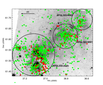
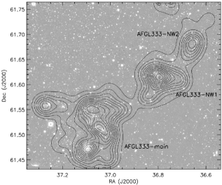
Figure 9.— left: Spatial distribution of candidate YSOs identified within AFGL333 overlayed on the 4.5 $\mu$m Spitzer-IRAC image. Class I, Class II YSOs are represented in red and green, respectively. The important stellar groups identified within AFGL333 are labeled and the circles around them represent their estimated sizes. right: Surface density map of YSOs within AFGL333 overlayed on the NEWFIRM $K_{s}$-band image. Surface density was calculated using the 6 nearest neighbours. Contours correspond to YSO surface densities of 5 to 44 stars pc^-2 with an interval of 3 stars pc^-2.

5.2. Properties of setllar groups in AFGL333: Disk fraction and Ages

In this subsection we discuss the disk fraction and ages of three stellar groups identified within AFGL333. Though these individual groups have sub-clusters in it (Fig. 9), due to the limited sensitivity and spatial resolution of the present study, we consider them as single group of YSOs. Hence the properties of the individual groups studied below should be considered as their average properties. The statistics of various sources within individual groups as well as in a nearby control field region are summarized in Table 4.

Table 4Derived cluster parameters

Group	Radius	Total	Class I	Class II	N(I/II)	disk fraction
ID		stars				($A_{V}$ corrected)
AFGL333-main	6.0′ (3.5pc)	1647	58	372	0.16	61%
AFGL333-NW1	3.5′ (2.0pc)	615	14	158	0.09	58%
AFGL333-NW2	3.0′ (1.7pc)	378	5	66	0.08	50%
Control field	3.0′ (1.7pc)	279	-	-	-

An approximate age estimation of individual groups is difficult from the color magnitude diagram because the luminosity scatter is large due to NIR excess and extinction (eg. Fig. 8). An alternate way to roughly infer the ages of young clusters is from the disk fraction since the fraction of sources surrounded by circumstellar disks strongly depends on the age of the system (Haisch et al. 2001; Hernández et al. 2008; Fang et al. 2013). From Spitzer-IRAC studies of young clusters, the average disk fractions at different cluster ages are 75% at $\sim$ 1Myr, 50% at $\sim$ 2Myr, 20 % at $\sim$ 5Myr and 5% at $\sim$ 10 Myr (Williams & Cieza, 2011).

The census of the diskless Class III sources is unknown in this survey because of their lack of IR-excess,and X-ray or spectroscopic data are not available to identify them. In order to account for the total number of Class III sources, the statistics of the point sources in a nearby control field is used (Table 4). We subtracted the field star contribution from the individual groups, after scaling the number of sources in the control field to the areas of individual groups. The remaining number of sources is considered as the total member stars (disk and diskless) within each region. However, a direct subtraction of field stars would overestimate the disk fraction because the background sources within the sub-regions are seen through the intervening molecular cloud, whereas the control field stars are only affected by the normal interstellar reddening. To account for differential extinction between AFGL333 and our control field, we synthesized the background stellar population using the Besançon Galactic model of stellar population (Robin et al., 2003), for normal interstellar reddening and for $A_{V}$= 10 mag. Here we assume $A_{V}$= 10 mag as the average reddening within AFGL333 (see Section 3). We find that $\sim$ 85% of field stars will be seen through the cloud in $L$-band when compared to the total number of field stars in a cloud free region.

Table 4 provides the disk fraction of individual clusters. After accounting for extinction, the disk fraction is estimated to be $\sim$ 61%, 58% and 50% for AFGL333-main, AFGL333-NW1 and AFGL333-NW2, respectively. The average disk fraction vs age trend reported in the literature (e.g. Haisch et al. 2001; Hernández et al. 2008; Fang et al. 2012, 2013) suggests $\sim$ 50% of the stars in a given region should have lost their disks around 2-3 Myr. The disk fraction estimated for AFGL333 matches with star forming regions of age $\sim$ 2-3 Myr.

Another way to infer the relative ages of different cluster populations is from the Class I/II ratio, given the different median lifetimes for these two evolutionary phases (i.e, 0.44 Myr for Class I; 2 Myr for Class II; Evans et al. 2009). The ratio of Class I to Class II sources should decrease with the average age of the region (Beerer et al. 2010; Myers 2012). Within the sub-clusters of AFGL333, the class I/II ratios are $\sim$ 10% (see Table 4), indicating a low fraction of embedded stellar population. The Class I/II value for AFGL333 is comparable to the Vul OB1 (Billot et al., 2010) and Cygnus X North (Beerer et al., 2010), which are at similar distances to AFGL333. After scaling to the distance of AFGL333, the Class I/II ratio of some of the c2d clouds (Evans et al., 2009) and young clusters (Gutermuth et al., 2009) agrees with that of AFGL333-main (Kim et al., 2015). Assuming the same distance, all of the above regions and AFGL333 have similar Class I/II values, which indicates that they are similar in age ($\sim$ 2-3 Myr) or at a similar evolutionary stage.

As evident in Fig. 9, the number of Class I sources increases towards the center of the ridge. The Class I/II ratio ($\sim$ 1.3; 32 Class I, 24 Class II) within 2 pc² of ridge is high when compared to $\sim$ 0.08 in the rest of the cloud. Therefore the ridge is likely young ($<$ 1 Myr, Evans et al. 2009; Samal et al. 2015) while other regions within AFGL333 are older. This is in agreement with Rivera-Ingraham et al. (2011), who found that the stellar group associated with the molecular ridge is relatively younger than that of other stellar groups.

The above methods to estimate the age of the region should be taken with caution. The disk fraction can only be used as a rough age indicator because of large scatter in this relation due to several factors including the incompleteness of different surveys, differences in diagnostic methods used for disk fraction estimation and the effects that age spread, metallicity, UV radiation and stellar density may have on the disk evolution (Soderblom et al. 2014; Spezzi et al. 2015). Similarly, the Class I/II ratio is sensitive to the age spreads and also due to the uncertainty in the Class 0/I lifetimes. Moreover the disk fraction or Class I/II ratios of AFGL333 are the average values of the individual groups, which contains several sub-groups and are probably at various evolutionary stages.

5.3. Estimation of cloud mass

In Section 3, we constructed an extinction map of resolution 20^′′ for the AFGL333 region using the deep NIR data. From the extinction map and assuming a distance of 2.0 kpc, the cloud mass of AFGL333 is estimated using following relation M = $m_{H}$ $\mu_{H_{2}}$ $A$ $\Sigma$ $N(H_{2})$, where $m_{H}$ is the mass of hydrogen, $\mu_{H_{2}}$ is the mean molecular weight per $H_{2}$ molecule, $N(H_{2})$ is the column density and A is the pixel area. The value of $\mu_{H_{2}}$ used is 2.8 (Kauffmann et al., 2008). We convert the extinction in magnitude to column density using the relation $N(H)$/$A_{V}$ = 1.87 $\times$ 10²¹ cm^-2mag^-1 (Bohlin et al., 1978). This expression has been derived assuming $R_{V}$ = 3.1. After subtracting the foreground reddening, the column density of all pixels within AFGL333 is integrated to estimate the cloud mass. The estimated mass within AFGL333 area is $\sim$ 1.7 $\times$ 10⁴ $M_{\odot}$ which is consistent with the mass ($\sim$ 1.8 $\times$ 10⁴ $M_{\odot}$) estimated from the CO based column density map. We explain below the various uncertainties involved in the mass estimation from the NIR based extinction map and infer a corrected mass.

The major uncertainty in the estimation of cloud mass comes from the assumption of standard extinction law in the complex. Use of $R_{V}$ = 3.1 would overestimate the cloud mass by a factor of 1.4 when compared to $R_{V}$ = 5.5 (i.e., $N_{H}$/$A_{V}$ = 1.37 $\times$ 10²¹ cm^-2mag^-1, Heiderman et al. 2010; Evans et al. 2009; Draine 2003). Similarly, there is an intrinsic uncertainty up to $\sim$ 2 mag in every pixel of $A_{V}$ map (see Section 3). Also, the estimated cloud mass should be considered as a lower limit, since the measured column density from extinction map is limited by the detection limit of our NIR observations (i.e., $A_{V}$ $<$ 26 mag), especially towards the ridge, where the column density is high.

A small fraction of the total area of AFGL333 (i.e., $\sim$ 4 %), close to the center of the ridge, has an average column density $\sim$ 3.7 $\times$ 10²² cm^-2 (Higuchi et al., 2013). The mass of the molecular clump around the ridge was measured as $\sim$ 4.2 $\times$ 10³ M_⊙ by Higuchi et al. (2013) using C¹⁸O(J=1-0) line emission. Including the extra cloud mass which is underestimated in our extinction map, the total mass of the AFGL333 region is estimated to be $\sim$ 2.1 $\times$ 10⁴ $M_{\odot}$. The intrinsic uncertainty of $\sim$ 2 mag in $A_{V}$ measurement (see Section 3) is added to the extinction map in order to estimate the upper limit of the cloud mass, which is obtained as $\sim$ 2.6 $\times$ 10⁴ $M_{\odot}$. The cloud mass estimate of AFGL333 per area is consistent with that of Rivera-Ingraham et al. (2013). AFGL333 region contains $\sim$ 10% of the total mass of the entire W3 complex measured from ¹²CO(J=3-2), ¹³CO(J=3-2) and C¹⁸O(J=3-2) maps ($\sim$ 4.4 $\times$ 10⁵ $M_{\odot}$; Polychroni et al. 2012) and from the Herschel Far-IR dust emission map ($\sim$ 2.3 $\times$ 10⁵ $M_{\odot}$; Rivera-Ingraham et al. 2013).

We also calculated the cloud masses around individual stellar groups by integrating the cloud density within their respective area, after accounting for the cloud mass towards the ridge and the intrinsic uncertainty in extinction measurements (see Table 5).

5.4. Star formation efficiency and rate

Star formation efficiency (SFE) and rate are two fundamental physical parameters to characterize how the cloud mass is converted into stars. We derive the star formation efficiency of the region by comparing the mass of the gas reservoir ($M_{cloud}$), with the mass that has turned into stars ($M_{star}$) during the last few million years. i.e., SFE = $M_{star}$/$(M_{star}+M_{cloud}$) (Myers et al., 1986).

In order to estimate the stellar mass, the total number of stars detected within individual stellar groups and brighter than the completeness limit ($K_{s}<$ 17 mag, for $>$ 0.2 M_⊙ at $A_{V}<$ 10 mag) is used. We subtracted the extinction corrected field star contribution from individual groups (see Section 5.2). The remaining stars are normalized to the Kroupa IMF with $\alpha$ = 2.3 for $M$ $>$ 0.5 $M_{\odot}$ and $\alpha$ = 1.3 for $M$ $<$ 0.5 $M_{\odot}$ (Kroupa, 2002). The total stellar mass is derived by extrapolating down to hydrogen burning limit (0.08 $M_{\odot}$). The estimated stellar mass within each stellar groups and total stellar mass of three groups are given in Table 5.

The overall star formation efficiency for various stellar groups ranges between $\sim$ 3% - 11% . Their combined star formation efficiency is $\sim$ 4.5%. In general, the star formation efficiency of AFGL333 is consistent with that of majority of the nearby star forming regions in the Galaxy (i.e., 3–6%, Evans et al. 2009).

Table 5Cluster parameters

Group	area	$M_{cloud}^{a}$	$M_{star}$	SFE	SFRb	$\Sigma_{gas}$	$\Sigma_{SFR}$
ID	(pc2)	($M_{\odot}$)	($M_{\odot}$)		($M_{\odot}$ Myr-1)	($M_{\odot}$ pc-2)	($M_{\odot}$ Myr-1pc-2)
AFGL333-main	38.0	7100 - 7700	248	0.03 - 0.03	78 - 118	187 - 203	2.1 - 3.1
AFGL333-NW1	12.8	940 - 1150	123	0.10 - 0.12	30 - 45	73 - 90	2.3 - 3.5
AFGL333-NW2	9.5	660 - 810	69	0.08 - 0.10	20 - 31	69 - 85	2.2 - 3.3
Total	60.3	8700 - 9700	440	0.04 - 0.05	128 - 192	144 - 161	2.1 - 3.2

^a The cloud mass is estimated after incorporating the uncertainty in extinction measurement
^b SFR is calculated for ages 2 and 3 Myr

Star formation rate (SFR) is the rate at which the gas in a cloud turns into stars. SFR can be estimated using the relation, SFR = $M_{cloud}\times$ SFE/$t_{SF}$, where $t_{SF}$ is the duration of star formation. The star formation rates of the individual stellar groups as well as for the entire region are estimated by assuming the duration of star formation in AFGL333 is $\sim$ 2 - 3 Myr (see Table 5). On average, the AFGL333 region is forming $\sim$ 130 - 190 M_⊙ of stars every Myr. The star formation rate varies with gas density ($\Sigma_{gas}$), i.e., the low density regions have star formation rates less than the high density regions within AFGL333 (see Table 5). This result agrees with the analysis of nearby molecular clouds (Lada et al. 2010; Gutermuth et al. 2011), Spitzer-c2d/GB clouds (Heiderman et al., 2010) and galactic massive dense clumps (Wu et al., 2010), where they find a linear relation between star formation rate and local gas density.

The star formation rate per unit surface area ($\Sigma_{SFR}$), i.e. the density of star formation, has been considered as a more generalized representation of the star formation rate of a given region (Heiderman et al., 2010). $\Sigma_{SFR}$ for individual groups within AFGL333 has been estimated by considering the area of each cluster over which the cloud mass is measured (see Table 5). The derived values of $\Sigma_{SFR}$ for individual groups and the total $\Sigma_{SFR}$ for the entire region as well as the corresponding cloud gas surface density ($\Sigma_{gas}$) are listed in Table 5. For AFGL333, the average values of $\Sigma_{gas}$ and $\Sigma_{SFR}$ are $\sim$ 140 - 160 $M_{\odot}$ pc^-2 and $\sim$ 2 - 3 $M_{\odot}$ Myr^-1pc^-2, respectively. The above estimates of stellar mass and various parameters are subjected to bias introduced by the unresolved binary/multiple systems. About 75% of the stars that make up the standard IMF are M type stars which have a binary fraction of $\sim$ 20-40% (Lada 2006; Basri & Reiners 2006). Assuming $\sim$ 30% of member stars in AFGL333 are unresolved binaries, the actual number of forming stars, the star formation efficiency and star formation rates would be increased by about the same factor (Evans et al., 2009).

6. Discussion

The W3 giant molecular cloud complex has long been discussed as a classic example of induced or triggered star formation (e.g., Lada et al. 1978; Oey et al. 2005). The expansion of the nearby W4 super bubble may have created the ‘high density layer (HDL)’ of molecular gas, at its western periphery. W3 Main, W3 (OH) and AFGL333 are the three main star forming sites identified within the HDL. W3 Main and W3 (OH) are located at the edges of the cavity created by the young cluster IC 1795. It has been proposed that the star formation within W3 Main and W3 (OH) are induced by IC 1795 (e.g., Oey et al. 2005; Román-Zúñiga et al. 2015). According to Rivera-Ingraham et al. (2013), in W3 Main the triggering processes work at local (sub-parsec) scales, with high mass stars acting to confine and compress material, enhancing the efficiency for the formation of new high mass stars by making convergent flow. In converging flows, the formation of new stars in cluster can be facilitated for an extended period as the structures will continue drain matter until the matter in their reservoirs get depleted. As pursued by Rivera-Ingraham et al. (2013, 2015), the combined effects of constructive feedback and converging flow could lead to the unique population of high-mass stars and clusters in W3 Main. W3 Main and AFGL333 are possibly different in terms of the cloud density and dynamics. W3 Main perhaps had initial high density which resulted to become very high mass stars in it whereas AFGL333 does not have density as high as W3 Main.

Using deep NIR and Spitzer data sets, we obtained the census of young stellar objects within AFGL333 as well as its cloud structure and mass. In this section, we compare the star formation rate density and gas density estimated for AFGL333 with nearby low mass clouds as well as high mass regions. We also compare these parameters between W3 Main and AFGL333, and discuss whether the differences between them have any implication due to the various star formation scenarios proposed in these two regions.

6.1. Comparison of AFGL333 with other star forming regions and W3 Main

The surface density of star formation rate ($\Sigma_{SFR}$) ranges from 0.1 and 3.4 M_⊙ Myr^-1 pc^-2 for a sample of 20 local low mass star forming regions (Heiderman et al., 2010). Similarly, Evans et al. (2009) reported the values between 0.6 - 3.2 M_⊙ Myr^-1 pc^-2, for the nearby low mass Spitzer-c2d/GB clouds. Both of those studies have used the NIR extinction map for cloud mass estimation, similar to the method followed in this study. The $\Sigma_{SFR}$ measured towards AFGL333 ($\sim$ 2 - 3 $M_{\odot}$ Myr^-1pc^-2; table 5) is comparable to that of these low mass regions.

We also compare the $\Sigma_{SFR}$ of AFGL333 with the high mass star forming regions such as NGC 6334, W43 and IRDC G035.39-00.33 (Willis et al. 2013; Motte et al. 2012). NGC 6334 is located at a similar distance ($\sim$ 1.6 kpc) and the YSO identification and cloud mass estimation from extinction map are calculated in a similar method as in AFGL333. $\Sigma_{SFR}$ of NGC 6334 is of $\sim$ 13.0 M_⊙ Myr^-1 pc^-2, factor of $\sim$ 6 higher than AFGL333. For W43 and IRDC G035.39-00.33, $\Sigma_{SFR}$ is as high as $\sim$ 10-100 M_⊙ Myr^-1 pc^-2 (Motte et al. 2003, 2012).

W3 Main and AFGL333 are part of the same cloud complex and have similar sizes ($\sim$ 0.45 deg², Lada et al. 1978; Rivera-Ingraham et al. 2013) and ages ($\sim$ 2-3 Myr, (Bik et al., 2012). W3 Main is the most active star-forming region in the entire W3 complex, which contains more than 10 Hii regions of various evolutionary status (Tieftrunk et al. 1997; Ojha et al. 2004, 2009) and more than 15 massive stars of spectral type O3V-B0V (Bik et al., 2012) within the central 5.4 pc² area. The central area of W3 Main has cloud density as high as $\sim$ 2 $\times$ 10²³ cm², with two clumps of masses 1700 and 800 M_⊙, respectively (Rivera-Ingraham et al., 2013). These values satisfy the conditions for high mass star formation, which means that W3 Main may continue forming massive stars in the future. Unlike W3 Main, at present AFGL333 does not have the column density above the threshold for the formation of massive stars (i.e., N${}_{H_{2}}$ $\sim$ 1.8 $\times$ 10²³ cm²; Krumholz & McKee 2008; Rivera-Ingraham et al. 2013). So far only one massive star of spectral type B0.5V has been identified within AFGL333 (Hughes & Viner, 1982).

For W3 Main, the SFE has been estimated as $\sim$ 44% by Bik et al. (2012) for an area $\sim$ 6.5 pc² around the core of W3 Main. However, this is to be considered as an upper limit, as the cloud mass is estimated from ¹³CO and C¹⁸O observations (Dickel 1980; Thronson 1986), where only the dense part of the region would have contributed to the cloud mass estimate. Assuming the age of W3 Main as 2-3 Myr (Bik et al., 2012), the $\Sigma_{SFR}$ comes out to be $\sim$ 110 - 160 M_⊙ Myr^-1 pc^-2, factor of $\sim$ 50 higher than that of AFGL333.

In spite of being part of the same giant molecular cloud complex with similar size and age, W3 Main and AFGL333 differ substantially in their level of star forming activities. This is similar to the star formation rate variation observed among the most-studied nearby active star formation sites in the Orion sub-regions, which includes regions such as ONC, L1630, L1641 etc. These clouds each have masses (a few $\times$ 10⁴ M_⊙) comparable to that of AFGL333. The star formation rate in L1630 is known to be a factor of 2 to 7 lower than that of the nearby L1641, despite having a very similar total reservoir of molecular material (Meyer et al. 2008; Spezzi et al. 2015). One possible explanation is the difference in the spatial distribution of dense gas between the two clouds (Meyer et al., 2008). Similarly, W3 Main has a much larger reservoir of star forming gas in a compact area, possibly formed by the convergent constructive feedback scenario proposed by Rivera-Ingraham et al. (2013), which causes the enhanced star formation rate when compared to AFGL333 (e.g., Gutermuth et al. 2011; Lada et al. 2010). The cloud distribution as well as the star formation activities within W3 Main is similar to that of the other high mass star forming regions such as NGC 6334 and W43, whereas, AFGL333 resembles other low mass star forming regions.

6.2. Implications for triggered star formation in AFGL333

Observational signposts of triggering in star forming regions include pillar or cometary type structures protruding towards the massive stars, YSOs coinciding with bubble rim/shells, age gradient between the YSOs located outside and inside the bright rim clouds, temperature gradient etc. (e.g., Chauhan et al. 2011; Jose et al. 2013; Pandey et al. 2013). The bright rim cloud BRC 5 is located towards the southeast of AFGL333 and several short pillars extend into the W4 bubble interior. The winds and radiation emanating from young massive stars of W4 have sculpted these elongated elephant trunks out of the surrounding molecular material. Based on an optical photometric analysis, Panwar et al. (2014) reported that the YSOs located within the bright rim of BRC 5 are younger than those YSOs outside the rim. Similarly, the dust temperature map from Herschel observations shows that the temperature is high ($\sim$ 22 K) near the ionization front at BRC 5, and is relatively low ($<$ 14 K) near the ridge (Rivera-Ingraham et al., 2013). The higher temperature at the ionization front indicates that it has been heated by the strong radiation from W4. The above examples are some of the classical signatures of triggered star formation that are seen at the eastern edge of AFGL333.

Triggered star formation can be defined in many ways, such as a temporary or long term increase in the star formation rate, an increase in the final star formation efficiency or an increase in the total final number of stars formed (Dale et al., 2015). Our observational analysis shows that the star formation efficiency and rate within AFGL333 is comparable to nearby low mass star forming regions. Stellar feedback has apparently not enhanced the star formation efficiency of AFGL333. If the massive OB stars of W4 had strong influence on AFGL333, then the closer region (AFGL333-main) should be more affected than the distant region (AFGL333-NW2). However, we find almost similar ages, star formation efficiencies and star formation rates for the sub-clusters of AFGL333.

Our analysis suggests that sequential star formation, which one would expect for a cloud under the influence of external ionizing photons, is not the prime mechanism of star formation in AFGL333. Star formation influenced by external feedback does not seem to have propagated throughout the cloud within AFGL333. Although individual YSOs at the tips of the small clouds (e.g. BRC 5, pillars) might be triggered, their contribution to the overall star formation efficiency and rate of the entire cloud is low. The star formation in these sub-clusters could have started due to the primordial cloud collapse. The ionization and shock front of the W4 bubble may have stalled at the east of AFGL333, giving the impression of triggering.

We would like to remind the readers that the star formation parameters of AFGL333 are the average properties of the three major stellar groups (see Section 5.1), which comprise sub-clusters of various evolutionary status, environments and external conditions. Due to the limited sensitivity and spatial resolution of the data sets in this study, we do not segregate the different populations within AFGL333-main. Hence we are unable to detect any local triggering process acting in scales of $\sim$ 1.5 pc or less. In conclusion, W4 Hii region appears to have little or no effect on the overall, averaged star formation activity within AFGL333, except that for the easternmost regions that associated with BRC 5.

Disentangling triggered star formation from spontaneous star formation requires precise determination of proper motion and ages of individual sources (Dale et al., 2015). Even if we assume that some triggering is going on at the eastern side of the AFGL333 cloud, the overall effect of feedback from W4 on the properties of the entire AFGL333 cloud is low. Numerical simulations by Dale & Bonnell (2012) also show that stellar feedback may simultaneously enhance or suppress star formation and may not have a strong effect on the overall star formation efficiency. Detailed observational studies of a large sample of star forming regions are needed to strengthen the hypothesis that feedback does not measurably affect the global star formation rate and efficiency.

7. Summary

The W3 giant molecular cloud complex is one of the most active massive star forming regions in the outer Galaxy. W3 Main, W3 (OH) and AFGL333 are the major sub-regions within W3. This complex has been subject to numerous investigations as it is an excellent laboratory for studying the feedback effect from massive stars of the nearby W4 super bubble. The low mass stellar content of AFGL333 was poorly explored until this study.

We analyzed the deep $JHK_{s}$ observations complimented with Spitzer-IRAC-MIPS observations to unravel the low mass stellar population as well as to understand the cloud structure and star formation activity within AFGL333. Based on the NIR and mid-IR colors, we identified 812 candidate YSOs in this region, of which 99 are classified as Class I and 713 as Class II sources. The survey is complete down to $\sim$ 0.2 M_⊙. This survey increases the census of YSO members of the region by a factor $>$3 compared to previous studies. The spatial distribution and the stellar density analysis shows that a majority of the candidate YSOs are located mainly within three stellar groups, named as AFGL333-main, AFGL333-NW1 and AFGL333-NW2. The disk fraction estimated within three stellar groups are $\sim$ 50–60%.

Using NIR data as well as CO based column desnity map, extinction maps across AFGL333 is constructed in order to understand the cloud structure as well as to estimate the cloud mass of the region. Combining the stellar mass with cloud mass, average star formation efficiency of the region has been estimated as $\sim$ 4.5% and star formation rate as $\sim$ 130 - 190 M_⊙ Myr^-1. The star formation rate density ($\Sigma_{SFR}$) measured within AFGL333 is $\sim$ 2 - 3 $M_{\odot}$ Myr^-1pc^-2.

We compared the star formation activity of AFGL333 with that of nearby low mass and high mass star forming regions as well as with W3 Main. The star formation rate density of AFGL333 is similar to the nearby low mass star forming regions but is a factor of $\sim$ 50 lower than that of W3 Main. Currently AFGL333 is not dense enough to form massive stars. On the other hand, the star formation activity within W3 Main is comparable to other high mass star forming regions of the Milky Way and the region is still dense enough to form many more massive stars in future.

Though we observe some of the classical signs of triggering such as pillars, bright rim cloud etc. towards the eastern edge of AFGL333, we find no evidence to suggest that stellar feedback has influenced the global star formation activity within AFGL333. The star formation activity in AFGL333 and W3 Main are different most likely due to the difference in the gas density within them as well as due to the differences in the feedback mechanisms in these two regions. However, detailed studies of a large sample of externally influenced regions are essential in order to quantify this statement.

References

- Allen et al. (2008) Allen, T. S., Pipher, J. L., Gutermuth, R. A., et al. 2008, ApJ, 675, 491
- Basri & Reiners (2006) Basri, G., & Reiners, A. 2006, AJ, 132, 663
- Beerer et al. (2010) Beerer, I. M., Koenig, X. P., Hora, J. L., et al. 2010, ApJ, 720, 679
- Bica et al. (2003) Bica, E., Dutra, C. M., & Barbuy, B. 2003, A&A, 397, 177
- Bieging & Peters (2011) Bieging, J. H., & Peters, W. L. 2011, ApJS, 196, 18
- Bik et al. (2012) Bik, A., Henning, T., Stolte, A., et al. 2012, ApJ, 744, 87
- Billot et al. (2010) Billot, N., Noriega-Crespo, A., Carey, S., et al. 2010, ApJ, 712, 797
- Bisbas et al. (2011) Bisbas, T. G., Wünsch, R., Whitworth, A. P., Hubber, D. A., & Walch, S. 2011, ApJ, 736, 142
- Black & van Dishoeck (1987) Black, J. H., & van Dishoeck, E. F. 1987, ApJ, 322, 412
- Bohlin et al. (1978) Bohlin, R. C., Savage, B. D., & Drake, J. F. 1978, ApJ, 224, 132
- Bressan et al. (2012) Bressan, A., Marigo, P., Girardi, L., et al. 2012, MNRAS, 427, 127
- Cardelli et al. (1989) Cardelli, J. A., Clayton, G. C., & Mathis, J. S. 1989, ApJ, 345, 245
- Casertano & Hut (1985) Casertano, S., & Hut, P. 1985, ApJ, 298, 80
- Chapman et al. (2009) Chapman, N. L., Mundy, L. G., Lai, S.-P., & Evans, II, N. J. 2009, ApJ, 690, 496
- Chauhan et al. (2011) Chauhan, N., Ogura, K., Pandey, A. K., Samal, M. R., & Bhatt, B. C. 2011, PASJ, 63, 795
- Chavarría et al. (2008) Chavarría, L. A., Allen, L. E., Hora, J. L., Brunt, C. M., & Fazio, G. G. 2008, ApJ, 682, 445
- Dale & Bonnell (2012) Dale, J. E., & Bonnell, I. A. 2012, MNRAS, 422, 1352
- Dale et al. (2013) Dale, J. E., Ercolano, B., & Bonnell, I. A. 2013, MNRAS, 430, 234
- Dale et al. (2015) Dale, J. E., Haworth, T. J., & Bressert, E. 2015, MNRAS, 450, 1199
- Dickel (1980) Dickel, H. R. 1980, ApJ, 238, 829
- Draine (2003) Draine, B. T. 2003, ARA&A, 41, 241
- Elmegreen & Lada (1977) Elmegreen, B. G., & Lada, C. J. 1977, ApJ, 214, 725
- Evans et al. (2009) Evans, II, N. J., Dunham, M. M., Jørgensen, J. K., et al. 2009, ApJS, 181, 321
- Fang et al. (2013) Fang, M., Kim, J. S., van Boekel, R., et al. 2013, ApJS, 207, 5
- Fang et al. (2012) Fang, M., van Boekel, R., King, R. R., et al. 2012, A&A, 539, A119
- Fazio et al. (2004) Fazio, G. G., Hora, J. L., Allen, L. E., et al. 2004, ApJS, 154, 10
- Flaherty et al. (2007) Flaherty, K. M., Pipher, J. L., Megeath, S. T., et al. 2007, ApJ, 663, 1069
- Gutermuth et al. (2009) Gutermuth, R. A., Megeath, S. T., Myers, P. C., et al. 2009, ApJS, 184, 18
- Gutermuth et al. (2005) Gutermuth, R. A., Megeath, S. T., Pipher, J. L., et al. 2005, ApJ, 632, 397
- Gutermuth et al. (2011) Gutermuth, R. A., Pipher, J. L., Megeath, S. T., et al. 2011, ApJ, 739, 84
- Hachisuka et al. (2006) Hachisuka, K., Brunthaler, A., Menten, K. M., et al. 2006, ApJ, 645, 337
- Haisch et al. (2001) Haisch, Jr., K. E., Lada, E. A., & Lada, C. J. 2001, ApJ, 553, L153
- Heiderman et al. (2010) Heiderman, A., Evans, II, N. J., Allen, L. E., Huard, T., & Heyer, M. 2010, ApJ, 723, 1019
- Hernández et al. (2008) Hernández, J., Hartmann, L., Calvet, N., et al. 2008, ApJ, 686, 1195
- Higuchi et al. (2013) Higuchi, A. E., Kurono, Y., Naoi, T., et al. 2013, ApJ, 765, 101
- Hughes & Viner (1982) Hughes, V. A., & Viner, M. R. 1982, AJ, 87, 685
- Indebetouw et al. (2005) Indebetouw, R., Mathis, J. S., Babler, B. L., et al. 2005, ApJ, 619, 931
- Jose et al. (2012) Jose, J., Pandey, A. K., Ogura, K., et al. 2012, MNRAS, 424, 2486
- Jose et al. (2013) Jose, J., Pandey, A. K., Samal, M. R., et al. 2013, MNRAS, 432, 3445
- Kauffmann et al. (2008) Kauffmann, J., Bertoldi, F., Bourke, T. L., Evans, II, N. J., & Lee, C. W. 2008, A&A, 487, 993
- Kerton et al. (2008) Kerton, C. R., Arvidsson, K., Knee, L. B. G., & Brunt, C. 2008, MNRAS, 385, 995
- Kim et al. (2015) Kim, H.-J., Koo, B.-C., & Davis, C. J. 2015, ApJ, 802, 59
- Koenig et al. (2008) Koenig, X. P., Allen, L. E., Gutermuth, R. A., et al. 2008, ApJ, 688, 1142
- Kroupa (2002) Kroupa, P. 2002, Science, 295, 82
- Krumholz & McKee (2008) Krumholz, M. R., & McKee, C. F. 2008, Nature, 451, 1082
- Kulesa et al. (2005) Kulesa, C. A., Hungerford, A. L., Walker, C. K., Zhang, X., & Lane, A. P. 2005, ApJ, 625, 194
- Lada (2006) Lada, C. J. 2006, ApJ, 640, L63
- Lada et al. (1978) Lada, C. J., Elmegreen, B. G., Cong, H.-I., & Thaddeus, P. 1978, ApJ, 226, L39
- Lada et al. (2010) Lada, C. J., Lombardi, M., & Alves, J. F. 2010, ApJ, 724, 687
- Lada & Wilking (1984) Lada, C. J., & Wilking, B. A. 1984, ApJ, 287, 610
- Massi et al. (2015) Massi, F., Giannetti, A., Di Carlo, E., et al. 2015, A&A, 573, A95
- Mathis (1990) Mathis, J. S. 1990, ARA&A, 28, 37
- Meyer et al. (1997) Meyer, M. R., Calvet, N., & Hillenbrand, L. A. 1997, AJ, 114, 288
- Meyer et al. (2008) Meyer, M. R., Flaherty, K., Levine, J. L., et al. 2008, Star Formation in NGC 2023, NGC 2024, and Southern L1630, ed. B. Reipurth, 662
- Milam et al. (2005) Milam, S. N., Savage, C., Brewster, M. A., Ziurys, L. M., & Wyckoff, S. 2005, ApJ, 634, 1126
- Moore et al. (2007) Moore, T. J. T., Bretherton, D. E., Fujiyoshi, T., et al. 2007, MNRAS, 379, 663
- Motte et al. (2012) Motte, F., Bontemps, S., Hennemann, M., et al. 2012, in SF2A-2012: Proceedings of the Annual meeting of the French Society of Astronomy and Astrophysics, ed. S. Boissier, P. de Laverny, N. Nardetto, R. Samadi, D. Valls-Gabaud, & H. Wozniak, 45–50
- Motte et al. (2003) Motte, F., Schilke, P., & Lis, D. C. 2003, ApJ, 582, 277
- Myers (2012) Myers, P. C. 2012, ApJ, 752, 9
- Myers et al. (1986) Myers, P. C., Dame, T. M., Thaddeus, P., et al. 1986, ApJ, 301, 398
- Oey et al. (2005) Oey, M. S., Watson, A. M., Kern, K., & Walth, G. L. 2005, AJ, 129, 393
- Ojha et al. (2009) Ojha, D. K., Tamura, M., Nakajima, Y., et al. 2009, ApJ, 693, 634
- Ojha et al. (2004) —. 2004, ApJ, 608, 797
- Pandey et al. (2013) Pandey, A. K., Eswaraiah, C., Sharma, S., et al. 2013, ApJ, 764, 172
- Panwar et al. (2014) Panwar, N., Chen, W. P., Pandey, A. K., et al. 2014, MNRAS, 443, 1614
- Patten et al. (2006) Patten, B. M., Stauffer, J. R., Burrows, A., et al. 2006, ApJ, 651, 502
- Pineda et al. (2010) Pineda, J. L., Goldsmith, P. F., Chapman, N., et al. 2010, ApJ, 721, 686
- Polychroni et al. (2012) Polychroni, D., Moore, T. J. T., & Allsopp, J. 2012, MNRAS, 422, 2992
- Povich et al. (2013) Povich, M. S., Kuhn, M. A., Getman, K. V., et al. 2013, ApJS, 209, 31
- Probst et al. (2004) Probst, R. G., Gaughan, N., Abraham, M., et al. 2004, in Society of Photo-Optical Instrumentation Engineers (SPIE) Conference Series, Vol. 5492, Ground-based Instrumentation for Astronomy, ed. A. F. M. Moorwood & M. Iye, 1716–1724
- Rieke et al. (2004) Rieke, G. H., Young, E. T., Engelbracht, C. W., et al. 2004, ApJS, 154, 25
- Rivera-Ingraham et al. (2011) Rivera-Ingraham, A., Martin, P. G., Polychroni, D., & Moore, T. J. T. 2011, ApJ, 743, 39
- Rivera-Ingraham et al. (2013) Rivera-Ingraham, A., Martin, P. G., Polychroni, D., et al. 2013, ApJ, 766, 85
- Rivera-Ingraham et al. (2015) —. 2015, ApJ, 809, 81
- Robin et al. (2003) Robin, A. C., Reylé, C., Derrière, S., & Picaud, S. 2003, A&A, 409, 523
- Robitaille et al. (2008) Robitaille, T. P., Meade, M. R., Babler, B. L., et al. 2008, AJ, 136, 2413
- Román-Zúñiga et al. (2015) Román-Zúñiga, C. G., Ybarra, J. E., Megías, G. D., et al. 2015, AJ, 150, 80
- Rowan-Robinson et al. (2013) Rowan-Robinson, M., Gonzalez-Solares, E., Vaccari, M., & Marchetti, L. 2013, MNRAS, 428, 1958
- Ruch et al. (2007) Ruch, G. T., Jones, T. J., Woodward, C. E., et al. 2007, ApJ, 654, 338
- Sakai et al. (2006) Sakai, T., Oka, T., & Yamamoto, S. 2006, ApJ, 649, 268
- Samal et al. (2014) Samal, M. R., Zavagno, A., Deharveng, L., et al. 2014, A&A, 566, A122
- Samal et al. (2015) Samal, M. R., Ojha, D. K., Jose, J., et al. 2015, A&A, 581, A5
- Skrutskie et al. (2006) Skrutskie, M. F., Cutri, R. M., Stiening, R., et al. 2006, AJ, 131, 1163
- Soderblom et al. (2014) Soderblom, D. R., Hillenbrand, L. A., Jeffries, R. D., Mamajek, E. E., & Naylor, T. 2014, Protostars and Planets VI, 219
- Spezzi et al. (2015) Spezzi, L., Petr-Gotzens, M. G., Alcalá, J. M., et al. 2015, A&A, 581, A140
- Stetson (1987) Stetson, P. B. 1987, PASP, 99, 191
- Sugitani et al. (1991) Sugitani, K., Fukui, Y., & Ogura, K. 1991, ApJS, 77, 59
- Swaters et al. (2009) Swaters, R. A., Valdes, F., & Dickinson, M. E. 2009, in Astronomical Society of the Pacific Conference Series, Vol. 411, Astronomical Data Analysis Software and Systems XVIII, ed. D. A. Bohlender, D. Durand, & P. Dowler, 506
- Thronson (1986) Thronson, Jr., H. A. 1986, ApJ, 306, 160
- Tieftrunk et al. (1997) Tieftrunk, A. R., Gaume, R. A., Claussen, M. J., Wilson, T. L., & Johnston, K. J. 1997, A&A, 318, 931
- van Dishoeck & Black (1988) van Dishoeck, E. F., & Black, J. H. 1988, ApJ, 334, 771
- Walch et al. (2013) Walch, S., Whitworth, A. P., Bisbas, T. G., Wünsch, R., & Hubber, D. A. 2013, MNRAS, 435, 917
- Werner et al. (2004) Werner, M. W., Roellig, T. L., Low, F. J., et al. 2004, ApJS, 154, 1
- Whitney et al. (2008) Whitney, B. A., Sewilo, M., Indebetouw, R., et al. 2008, AJ, 136, 18
- Williams & Cieza (2011) Williams, J. P., & Cieza, L. A. 2011, ARA&A, 49, 67
- Willis et al. (2013) Willis, S., Marengo, M., Allen, L., et al. 2013, ApJ, 778, 96
- Wu et al. (2010) Wu, J., Evans, II, N. J., Shirley, Y. L., & Knez, C. 2010, ApJS, 188, 313
- Xu et al. (2006) Xu, Y., Reid, M. J., Zheng, X. W., & Menten, K. M. 2006, Science, 311, 54
- Zeidler et al. (2016) Zeidler, P., Preibisch, T., Ratzka, T., Roccatagliata, V., & Petr-Gotzens, M. G. 2016, A&A, 585, A49