Helical currents in metallic Rashba strips.

Abstract

We study the texture of helical currents in metallic planar strips in the presence of Rashba spin-orbit coupling (RSOC) on the lattice at zero temperature. In the noninteracting case, and in the absence of external electromagnetic sources, we determine by exact numerical diagonalization of the single-particle Hamiltonian, the distribution across the strip section of these Rashba helical currents (RHC) as well as their sign oscillation, as a function of the RSOC strength, strip width, electron filling, and strip boundary conditions. Then, we study the effects of charge currents introduced into the system by an Aharonov-Bohm flux for the case of rings or by a voltage bias in the case of open strips. The former setup is studied by variational Monte Carlo, and the later, by the time-dependent density-matrix-renormalization group technique. Particularly for strips formed by two, three and four coupled chains, we show how these RHC vary in the presence of such induced charge current, and how their differences between spin-up and spin-down electron currents on each chain, help to explain the distribution across the strip of charge currents, both of the spin conserving and the spin flipping types. We also predict the appearance of polarized charge currents on each chain. Finally, we show that these Rashba helical currents and their derived features remain in the presence of an on-site Hubbard repulsion as long as the system remains metallic, at quarter filling, and even at half-filling where a Mott-Hubbard metal-insulator transition occurs for large Hubbard repulsion.

I Introduction

There is an ongoing effort to take advantage of electron spin, in addition to its charge, for computing and information technologies, that has evolved into the new field of spintronics.prinz ; wolf ; zutic An important ingredient for spintronics devices, is the spin-orbit (SO) interaction, which provides the essential mechanisms for spin polarization and spin currents without the need of magnetic materials.awschalom ; sinovaRMP ; hoffmann13

In particular, at interfaces or surfaces of materials, the breaking of structure inversion symmetry, combined with the atomic spin-orbit interaction gives rise to the Rashba (or Bychkov-Rashba) spin-orbit coupling.rashba ; winkler It is well-known that the Rashba SO coupling (Rashba SOC or RSOC) in two-dimensional (2D) systems leads to the presence of pure spin currents, which are transversal to the direction of an applied charge current. This spin current is considered the intrinsic mechanism for the spin-Hall effect, which in many systems coexists and competes with extrinsic mechanisms. dyakonov ; Hirsch99 ; murakami06 ; sinova04 ; hoffmann13 ; vignale10 For finite width 2D systems such as wires or strips, this spin current is the origin of the phenomenon of spin accumulation.nikolic ; malshukov

The Rashba SOC in noninteracting 2D systems has been widely studied in first quantization,sinovaRMP ; bercioux where the finite width of strips is enforced by an harmonic potential or by an infinite potential well.erlingsson Much less has been done using second quantization on lattices, which provides a road to study the crossover from one-dimensional (1D) to 2D behavior,wenk ; riera ; gothassaad and to include realistic hoppings and SO couplings, as well as various types of electron correlations. These electron correlations are present in a number of surfaces and interfaces involving transition metal oxides, such as SrTiO₃hwang ; caviglia ; benshalom ; ykim ; caprara , particularly LaAlO₃/SrTiO₃,liu2014 ; banerjee ; sahin ; liu2014 ; khalsa ; bucheli and BaTiO₃, for example in the heterostructure BaTiO₃/BaOsO₃.seiji15

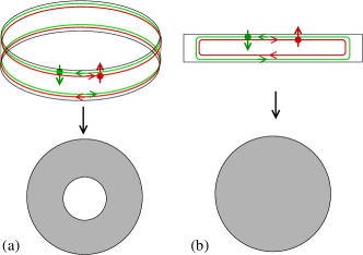
Figure 1: (Color online) Strips with (a) periodic boundary conditions, (b) and open boundary conditions along the longitudinal direction. In both cases there are open boundary conditions in the transversal direction. Conventional helical edge currents are shown for illustration. Each type of boundary condition is associated with a topology, as shown in the bottom figures.

In addition, second quantization and discrete lattices provide a scale of detail at a microscopic level, not accessible by continuum coarse grained techniques. The main physical property we want to address within this approach is the distribution of spin-up and spin-down electron currents that appear on strips due to the presence of edges, even in the absence of external electromagnetic potentials or fields. Helical edge currents where electrons with up and down spins move in opposite directions, such as those illustrated in Fig. 1, are well-known to be present in topological insulators of the quantum spin-Hall (QSH) type.bernevig ; sheng ; konig ; murakami ; kanemele ; okudakimura In the present work, we examine helical currents which appear in metallic planar strips in the presence of Rashba SOC. These helical currents are slowly decaying from the edges, and hence for a narrow strip, depending on the RSOC strength, they are present over all the section of the strip, not just on its edges as in the QSH case. This feature should be ultimately related to the fundamental difference between the Rashba SOC and the SO term that consists of two copies of the Haldane term and is the essence of the Kane-Mele modelkanemele This Haldane-like term of the Kane-Mele model, contrary to the Rashba SO term, conserves the $z$-component of the total spin, while breaking the time-reversal symmetry. We emphasize that what we call in the following Rashba helical currents (RHC) (defined in section II), are charge currents for each spin projection, and should not be confused with the already mentioned transversal spin currents, which are the ones related to the spin-Hall conductivity sinova04 ; nomura . In the absence of appplied magnetic or electric fields, at any point of the system, the spin-up Rashba helical current is exactly opposite to the spin-down one, and hence of course there is no net charge current.

One of the main features we will study is the texture of these Rashba induced helical currents, that is, the amplitude and sign oscillations of spin-up and spin-down electron currents on different chains as a function of their distance to the edge. These sign oscillations of helical currents were not so far detected experimentally, and hence did not receive too much theoretical attention, since in semiconductor devices the electron densities are low and RSOC is weak. However, some traces of this texture have been reported theoretically on studies on semiconductor wires.nomura2 ; nikolic New materials which are being considered for spintronic devices can perform at higher electron densities and present much larger RSOC, and hence the results of the present study may be relevant for such systems.seiji15 ; giantSO

Hence, the first purpose of the present article is to numerically determine the helical currents that appear due to the RSOC in two different systems, as shown in Fig. 1. We will first consider a ring geometry, that is, a strip with open boundary conditions (OBC) in the transversal direction and periodic boundary conditions (PBC) in the longitudinal one (Fig. 1(a)). Then, we will analyze a strip with full OBC (Fig. 1(b)), which could be regarded as an idealized version of the wires employed in spintronic devices.

In Section III we start our study with noninteracting systems in the absence of external electromagnetic sources. By using a combination of momentum and real-space techniques on both kinds of strips, the Rashba helical current distribution across the transversal section will be determined.

Next, we examine how the Rashba helical currents determine the net charge currents that appear in the presence of external electromagnetic sources. This part of the work, performed in Section IV, although certainly is the most relevant to physical systems or devices, could only be properly understood by resorting to the behavior of the Rashba helical currents studied in the previous section. In the case of rings, shown in Fig. 1(a), persistent currents can be induced by applying an Aharonov-Bohm flux through it. For strips such as those of Fig. 1(b), these currents are induced by connecting the trips to two leads with a voltage difference. As shown in Fig. 1, both kinds of strips belong in principle to different topologies and transport physics, and the purpose of the present work is to examine how the Rashba helical currents give rise to net longitudinal currents in both geometries.

In this second part of our effort, we will also include the effects of electron correlations, introduced by a Hubbard term in the Hamiltonian, again relevant for a number of recently introduced materials and devices, as mentioned before. So far, few studies have been accomplished in models including the Rashba SOC and Hubbard repulsion, and most of them were done on quasi-onedimensional lattices.riera ; gothassaad We will show that the analysis of RHC gives a fresh approach on this kind of correlated models, particularly on its transport properties.

II Model and methods

The Rashba SO Hamiltonian on the square lattice is given by: pareek ; sinova14

$$H_{R}=V_{SO}\sum_{l} [ c_{l+x,\downarrow}^{\dagger}c_{l,\uparrow}-c_{l+x,\uparrow}^{\dagger}c_{l,\downarrow}+i(c_{l+y,\downarrow}^{\dagger}c_{l,\uparrow}$$ (1)

$$+ c_{l+y,\uparrow}^{\dagger}c_{l,\downarrow})+H.c.]$$

and the total Hamiltonian is $H=H_{H}+H_{R}$, where

$$H_{H}=-t\sum_{<l,m>,\sigma}(c_{l,\sigma}^{\dagger}c_{m,\sigma}+H.c.)+U\sum_{l}n_{l,\uparrow}n_{l,\downarrow}$$ (2)

corresponds to the Hubbard model. The notation is standard. We will consider the isotropic case $t_{x}=t_{y}=t$, and $V_{SO,x}=V_{SO,y}=V_{SO}$, where $x$ ($y$) is the longitudinal (transversal) directions of the strips shown in Fig. 1, except otherwise stated. In the following, we have adopted the normalization, $\sqrt{t^{2}+V_{SO}^{2}}=1$, which we adopt as the unit of energy.

It is well-known that with the Rashba term, the $z$-projection of the total spin is no longer conserved, as well as the rotational symmetry in the spin space, while the time-reversal symmetry is still conserved.

In this work, we will study planar strips, with $L$ sites on the longitudinal direction, with periodic (Fig. 1(a)) or open (Fig. 1(b)), boundary conditions, and $W$ sites in the transversal direction, with OBC. In general, we will take $L\gg W$, so that the strips could be considered as $W$ coupled chains. The total number of sites is $N=L\times W$, and the total number of electrons, $N_{e}$, such that the filling is $n=N_{e}/N$. We will not consider the presence of impurities in our system.

The main quantities we are interested in are the currents associated to the hopping term in Eq. (2), termed the spin-conserving current, $J_{\sigma,x,y,\hat{\mu}}$, on each link between $(x,y)$ and $(x,y)+\hat{\mu}$, where $\hat{\mu}=\hat{x},\hat{y}$, which is the expectation value of the operator:

$$\hat{j}_{\sigma,x,y,\hat{\mu}}=it(c_{(x,y)+\hat{\mu},\sigma}^{\dagger}c_{(x,y),\sigma}-H.c.),$$ (3)

and the contribution from the RSOC term, which leads to the so-called spin-flipping current, $J_{SO,x,y,\hat{\mu}}$ which is the expectation value of a similar current operator that can be also similarly derived from Eq. (1) as the first order perturbation induced by a magnetic potential ${\bf A}$ added to Eq. (1) by the Peierls factors, $\gamma_{\hat{\mu}}\rightarrow\gamma_{\hat{\mu}}\exp{(-ieA_{\hat{\mu}})}$ (in units of $\hbar$), where $\gamma_{\hat{\mu}}$ are the appropriate coupling constant in the $\hat{\mu}$-direction. In the following we will also adopt units where $e=1$. Let us write down only the $x$-component of the SO current, which we will need for future discussions:

$$\hat{j}_{SO,x,y,\hat{x}} = -iV_{SO}[(c_{(x,y)+\hat{x},\downarrow}^{\dagger}c_{(x,y),\uparrow}-H.c.)-$$ (4)

$$( c_{(x,y)+\hat{x},\uparrow}^{\dagger}c_{(x,y),\downarrow}-H.c.)],$$

The expectation value of each term in parenthesis will be denoted as $J^{\prime}_{SO,x,y,\hat{x}}$ and $J^{\prime\prime}_{SO,x,y,\hat{x}}$, respectively, and similarly for the $y$-direction. The total current on each link is then $J_{tot,x,y,\hat{\mu}}=J_{\uparrow,x,y,\hat{\mu}}+J_{\downarrow,x,y,\hat{\mu}}+J_{SO,x,y,\hat{\mu}}$.

In the following we will compute and discuss the RHC as the ”spin-up currents” (”spin-down currents”), defined as the hopping currents $J_{\uparrow,x,y,\hat{x}}$ ($J_{\downarrow,x,y,\hat{x}}$) described above.

Spin accumulation is a well-known consequence of the spin-Hall effect in the presence of boundaries in the direction transversal to the direction of the charge current.nikolic ; malshukov ; riera That is, a charge current in the longitudinal direction that appears due to an external electromagnetic field, induces a transversal spin current, which then leads to spin polarization with opposite sign on opposite edges of the conducting strip. In principle, the spin accumulation is defined as the relative out-of-plane spin polarization between the two sides of the strip that is:

$$\Delta S^{z}=\sum_{1\leq j\leq W/2}S^{z}(j)-\sum_{W/2+1\leq j\leq W}S^{z}(j)$$ (5)

where $S^{z}(j)$ is the sum of the $z$-component of the electron spins on the chain $j$. For wide strips it is expected that the spin accumulation is concentrated on the strip edges as it was observed experimentally kato , although there is no consensus about the interpretation of these experimental results. In the narrow strips we will consider in Section IV, the spin polarization could take appreciable values across the whole section of the strip, so we will compute the polarization or spin accumulation on each chain, $\Delta S^{z}(j)=S^{z}(j)-S^{z}(W-j+1)$, $j=1,\ldots,W/2$. Hence the total spin acumulation can be expressed as $\Delta S^{z}=\sum_{1\leq j\leq W/2}\Delta S^{z}(j)$.

It has been noticed that spin polarization could also appear on strips due to the inverse spin galvanic effect (ISGE).wolf However, the current-induced spin polarization due to ISGE refers to in-plane ($x,y$) components of the spin, and has been studied in two-dimensional electron systems for varying $x,y$-directions of the currents.ganichev In contrast, we would like to emphasize that the spin polarization we compute and discuss in Section IV, is the out-of-plane ($z$) component related to the Spin-Hall effect on strips, and hence not to the ISGE.

For the noninteracting case, we solve numerically the Hamiltonian for a single electron. For the case of rings, Fig. 1(a), translation symmetry is preserved along the longitudinal direction ($x$-axis), while it is broken in the transversal direction ($y$-axis) due to the open BC. In this case, for each $k_{x}$ one has to solve a $2W\times 2W$ matrix, and the single particle eigenvalues and eigenvectors will be a function of $(k_{x},y,\sigma)$. In the absence of external electromagnetic fields, static currents on each chain both of the hopping and SO types, are computed by straightforward ground state averaging. These zero temperature results are presented in Section III.2.

For the geometry of Fig. 1(b), translation symmetry is broken also in the $x$ direction, so the single particle Hamiltonian matrix is formulated in real space, and it has dimensions $2N\times 2N$. In this case, one has in principle currents of spin-$\sigma$ electrons varying on each bond of the lattice, and in both directions, that is $J_{\sigma,x,y,\hat{\mu}}$. In Section III.3, only results for the currents at the center of the strip, $J_{\sigma,L/2,y,\hat{\mu}}$ will be discussed.

To deal with both external electromagnetic sources and nonzero electron-electron interactions, that is a finite value of $U$ in the Hubbard term, we will resort to much more involved many-body techniques to study the zero temperature behavior. For the case of periodic strips, we will study persistent currents along the ring, which are induced by piercing the ring by an Aharonov-Bohm flux.splettstoesser ; riera ; michetti The study of these currents is accomplished by a simple variational Monte Carlo (VMC) where configurations generated by a trial wave function which consists of a product of Slater determinants, are weighted by a Gutzwiller factor which depends on the number of double-occupied sites and the value of $U$.honghirsch ; giamarchi This technique allows us to study rings up to $W=4$, and electron-electron Hubbard repulsion up to $U=8$. Although this simple variational wave function underestimates the effect of $U$, the obtained results are qualitatively reliable as compared with those obtained by other techniques. Typically, for each set of parameters, and for each value of the Aharonov-Bohm flux, $\Phi$, we take Monte Carlo averages over $10^{6}$ sweeps.

In the case of an Aharonov-Bohm flux $\Phi$ piercing a ring, the total Hamiltonian $H_{R}+H_{H}$ has to be treated in the presence of Peierls factors in both the hopping and the RSOC terms along the $x$-direction, and $A_{\hat{x}}$ should be replaced by $\Phi/L$, where in the adopted units, $0\leq\Phi\leq 2\pi$. In this case, the ground state eigenvalue and eigenvector will be $E_{0}=E_{0}(\Phi)$, $\Psi_{0}=\Psi_{0}(\Phi)$, and hence the ground state expectation value of any physical quantity will also depend on $\Phi$.

To study currents induced by an external electric field, as well as electron correlations, in strips where OBC has been imposed also in the longitudinal direction, we resort to density matrix-renormalization group (DMRG) technique,schollwock which is in principle exact for static properties. In this case, currents appear as a time dependent feature after applying a voltage bias between the ends of the strip at a given time, after the iterative process has converged to the ground state. This first standard DMRG was carried out keeping up 800 states, and performing at least 14 sweeps, enough to achieve truncation errors of the order $O(10^{-6})$. The voltage bias is applied between the two halves of the strip in the longitudinal direction. Alternatively, we have applied this bias to the two ends of the strip without affecting the two central columns of the strip. The results obtained with both recipes are virtually identical. The voltage bias is small, $\Delta V=0.01$, so as to avoid strong nonequilibrium processes. This calculation requires an extension of the original DMRG algorithm, and the results are considered ”quasi-exact”. Among different DMRG approaches to deal with time evolution problemsschollwock ; feiginwhite ; alhassanieh , we choose the algorithm introduced by Manmanna et alMWNM-09 , which is a variant based on a Krylov-space representation of the time evolution operatorschmitteckert . Thereby, we are able to evolve systems with interactions involving many coupled chains, and obtain very accurate results for long time periods. We observed that using at each time slice $dt=0.1$, an Krylov base of $\sim 30$ states, the errors become smaller than the symbol sizes. For each strip, and for a given set of parameters, a single value for each type of current was taken as the amplitude of the first maximum reached in its time evolution, considered as an approximation of the expected plateau.

The application of computational techniques, particularly DMRG, is severely limited by the non-conservation of the total $S^{z}$, which implies a much larger Hilbert space for the system. The need to work with complex numbers, also implied by the Rashba SO coupling, further increases CPU time and memory requirements.

III Noninteracting case

III.1 Rashba helical currents

Let us start with the noninteracting case, $U=0$. As we will extensively show in the next sections, the RHC consist of spin-up or spin-down hopping currents which are exactly opposite on each chain across the strip section in the absence of external electromagnetic sources (fields or potentials). In addition, the currents for a given spin orientation, have opposite direction on chains symmetrically located with respect to the middle of the section, and their sign and strength vary over the section. In principle, counter propagating currents for each spin projection are guessed from general arguments similar to those leading to the prediction of the spin-Hall effectsinova04 ; okudakimura and which ultimately stem from requirements of time-reversal symmetry.

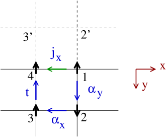
Figure 2: [Color Online] Schematic explanation of the origin of an effective current between sites ’1’ and ’4’, located at the system edge. $\alpha_{x}$, $\alpha_{y}$ and ’t’, indicate a Rashba SO movement along $x$ and $y$ directions, and a regular hopping respectively. Dashed lines indicate the possible processes that would be present in the bulk.

An alternative and instructive way of understanding the presence of these currents with opposite circulation of spin up and down electrons in the absence of external sources, can be done in real space in systems with Rashba SOC. At an effective level, these Rashba helical currents appear due a term in the Hamiltonian,

$$H_{\hat{\mu}}^{eff} \sim E_{\hat{\mu}}j_{\hat{\mu}}~{}~{}~{}~{}~{}~{}~{}~{}~{}~{}~{}~{}~{}~{}~{}~{}~{}~{}~{}~{}~{}~{}~{}~{}~{}~{}~{}~{}~{}~{}~{}~{}~{}~{}~{}~{}~{}~{}~{}~{}~{}~{}~{}~{}~{}~{}~{}~{}~{}$$

$$\sim i\lambda\sum_{l}[(c_{l+\hat{\mu},\uparrow}^{\dagger}c_{l+\hat{\mu},\downarrow}^{\dagger})(i\sigma^{z})\left(\begin{array}[]{c}c_{l,\uparrow}\\ c_{l,\downarrow}\end{array}\right)-H.c.]~{}~{}~{}$$ (8)

where $\hat{\mu}=\hat{x}$ or $\hat{y}$. The origin of this term is schematically shown in Fig. 2. A spin up electron at site ”1” could reach site ”4” by moving to site ”2” involving a spin-orbit process, and then to site ”3” with another SO process. Finally, it could reach site ”4” by an ordinary hopping. The full process would involve $\sigma^{y}\times\sigma^{x}=-i\sigma^{z}$, with a factor $\lambda$ proportional to $tV_{SO}^{2}$. An analogous process along sites ”2’ ” and ”3’ ” would have an opposite sign but this contribution is absent if that line is on a system edge. It is easy to see that the reverse process from ”4” to ”1” would lead to $\sigma^{x}\times\sigma^{y}=i\sigma^{z}$, thus providing the sign for the current in Eq. 8. In addition, processes involving more sites further away from the edge would contribute to that effective current on the edge, and also on legs located in the bulk due to the lack of compensation. If sites ”1” and ”4” belong to a leg located at $y$, processes through sites ”2” and ”3”, located at ”y+a” and process through sites ”2’ ” and ”3’ ”, located at ”y-a” would not cancel each other because legs ”y+a” and ”y-a” are in general not symmetric due to the proximity to the edge. For example, an effective current involving five sites would lead to a current between sites at the line next to the edge, and so forth. Of course, each hopping would on average have a probability of $(1-n/2)$, where $n$ is the electron filling, and assuming an equal number of electrons with up and down spins. Notice that for the so-called persistent helix state,bernevig2 where the Rashba and Dresselhaus,dresselhaus couplings are present with equal strength, the SO coupling is mediated by $\sigma^{x}-\sigma^{y}$ in both directions, and hence the effective terms illustrated in Fig. 2 turns out to be of the kinetic type, not of the current type.

Of course, for very large strip widths, processes with longer paths become unlikely, and far from the edges, processes with shorter path would cancel because legs become approximately equivalent. It is expected then that for large strip widths, these currents become essentially nonzero only at the strip edges. It will be tempting to assign the changes in sign and strength as a function of the distance of the chains to the edge, to a sort of Friedel oscillations, as it will be explored below.

It should also be noticed that the Rashba Hamiltonian Eq. (1) can be written in terms of currents, and the same kind of currents here studied could be the one seen in Ref. bovenzi, in the presence of impurities. That is, the impurities provide the breaking of translational symmetry that appear in our case due to the open boundaries of strip geometry.

Let us remark that according to the previous arguments, the RHC are of the hopping or spin-conserving type, given by Eq. (3), not of the SO or spin-flipping type, corresponding to Eq. (4).

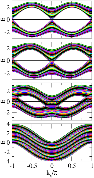
Figure 3: [Color Online] Energy bands as a function $k_{x}$ from top to bottom $V_{SO}/t=64$, 8.0, 2.0, and 0.4. $64\times 2000$ ring.

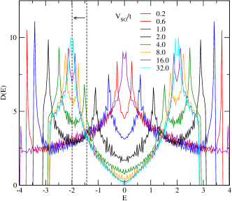
Figure 4: [Color Online] Density of states for the $64\times 2000$ ring for various values of $V_{SO}/t=64$, as indicated on the plot. The vertical dashed lines indicate the corresponding shift of the chemical potential for quarter filling.

In Fig. 3 the evolution of energy bands as a function of $k_{x}$ for various values of $V_{SO}/t$ is shown for rings. Results were obtained for the $64\times 2000$ ring. The top panel, corresponding to $V_{SO}/t\gg 1$, resembles the typical situation found in topological Dirac semimetalsmzhasan14 ; sunzhu ; baum2015 , with its characteristic Dirac nodes in the Fermi surface.dzero ; ynagaosa However, the purpose of the present work is to study the evolution of Rashba helical currents when $V_{SO}/t<1$, when the electron density is reduced below half-filling, and hence the physics of the topological Dirac semimetals is not relevant. As $V_{SO}/t$ is reduced, a more conventional band metallic behavior starts to appear. At $V_{SO}/t=0.4$, a single conduction band appears. It is interesting to note that the behavior shown in Fig. 3 is also similar to the one found in the ferromagnetic Kondo lattice model with Rashba SOC in 2D, with classical localized spins, for large values of the Hund coupling at quarter filling.meza Of course, this band structure is different to the one characteristic of QSH systems, reflecting the insulating character of the bulk, and the metallic character of the edge.kanemele ; laubach

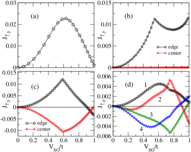
Figure 5: [Color Online] Spin-up currents for rings with (a) 2, (b) 3, (c) 4, and (d) 8 legs as a function of $V_{SO}/t$, and for different legs as indicated in the plots, $L=8000$, $n=0.5$. In (d), leg ”1” (”4”) corresponds to the edge (center).

The density of states for the same $64\times 2000$ ring in the noninteracting case is shown in Fig. 4, for various values of $V_{SO}/t$. It can be clearly seen a suppression of energy states around zero energy, corresponding to half-filling, as $V_{SO}/t$ is increased from 0.2 to 64. The vertical dashed lines indicate the corresponding shift of the chemical potential for quarter filling. Both Figs. 3 and 4 indicate a clear metallic behavior for all $V_{SO}/t$ and electron fillings.

III.2 Results on finite width rings

In this Subsection, we study planar rings such as the one depicted in Fig. 1(a). Since as said earlier, Rashba helical currents of spin-down electrons are exactly opposite to the spin-up ones, in the following we will only consider the spin-up electron currents on each chain. Moreover, since currents are spatially antisymmetric on chains with respect to the central longitudinal axis, we will only show the currents on the chains in half the section of the strip. Finally, due to translation invariance along the longitudinal direction, the currents will not depend on $x$. Hence, in all figures below, we will depict $J_{\uparrow,l}$, where $l=1,\ldots,W/2$ or $J_{\uparrow,\nu}$, where $\nu$ is the normalized distance of the chain to the edge, or chain depth, defined in such a way that $\nu=0$ at the edge and $\nu=1$ at the center, independently of the width $W$.

As discussed in Subsection III.1, the RHC, computed here as $J_{\uparrow,l}$, is a spin-conserving current, and spin-flipping currents are zero everywhere, which is remarkable since the SO coupling is needed to be nonzero in both directions for the RHC to exist. Moreover, notice that the conservation of the average charge on each site in the stationary regime (Kirchhoff’s law) is trivially satisfied for up and down spin electrons separately. This is compatible not only with the net SO currents being zero but also with the two contributions $J^{\prime}_{SO,x,y,\hat{\mu}}$ and $J^{\prime\prime}_{SO,x,y,\hat{\mu}}$, possibly being zero in both directions, $\hat{\mu}=\hat{x},\hat{y}$.

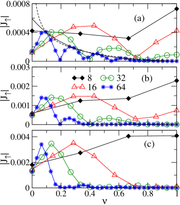
Figure 6: [Color Online] Absolute value of spin-up currents on each chain as a function of the depth of the chain ($\nu=0$, edge, $\nu=1$, center leg), (a) $V_{SO}/t=0.1$, (b) 0.2, (c) 0.4. $L=8000$ rings, $n=0.5$. Widths of the rings are indicated in the plot. The full (dashed) curves added in (a) correspond to exponential (power law) fits.

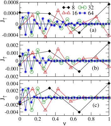
Figure 7: [Color Online] Spin-up currents on each chain as a function of the normalized depth of the chain for (a) $V_{SO}/t=0.1$, (b) 0.2, (c) 0.4. $L=8000$ rings, $W$ indicated on the plot, $n=0.5$.

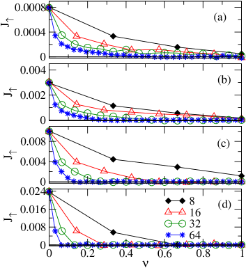
Figure 8: [Color Online] Spin-up current on each chain as a function of the depth of the chain ($\nu=0$, edge, $\nu=1$, center leg), for (a) $V_{SO}/t=0.1$, (b) 0.2, (b) 0.4, and (c) 0.8. $L=8000$ rings, $n=1$. Widths of the rings are indicated in the plot.

A direct evidence of the existence of the RHC and their predicted dependence with the square of $V_{SO}/t$ can be observed for strips of $W=2,3,4$ and 8 at $n=0.5$ at small $V_{SO}/t$, as shown in Fig. 5. This dependence becomes increasingly complex as the strip width is increased. For all $W$, there is a clear change of behavior around $V_{SO}/t\approx 0.5$, and for $W>2$, this behavior presents some cusps, which are typical of level crossings. In this, and in the following calculations in this Subsection, results for $L=800$ are virtuable indiscernible from those for $L=8000$, hence we are confident that the results are representative of the continuum limit in the longitudinal direction.

As suggested by the arguments of Subsection III.1, the RHC should concentrate near the strip edges, and only due to its slow decay from the edges, for small widths, the RHC appears to pervade the whole system. To examine this behavior we will consider a broad range of strip widths. As it can be seen in Fig. 6, the module of $J_{\uparrow}$ as a function of the chain’s depth $\nu$ indicates that only for $W\geq 16$ and $V_{SO}/t\geq 0.4$ it is apparent that these currents become essentially different from zero near to the strip edges. In general, wider strips have to be considered to show an edge-like behavior for smaller SO couplings. Two more features become apparent. First, consistently with the predictions of Subsection III.1, and with the behavior already shown in Fig. 5, the amplitude of these currents increases almost quadratically with $V_{SO}/t$, and second, and more interesting, $J_{\uparrow,\nu}$ presents an oscillatory behavior as a function of the chain depth, reminiscent of a Friedel oscillation behavior.

To quantify the decay of RHC as the chains are located away from the edge, we have fitted the curves for the widest ring, with $W=64$, with an exponential law, $J_{\uparrow,\nu}\sim\exp{(-B\nu)}$, and by a power law, $J_{\uparrow,\nu}\sim\nu^{(-B)}$. Results from these fits for $V_{SO}/t=0.1$ are shown in Fig. 6(a), and a systematic study of this fitting will be presented below in Fig. 9.

In Fig. 7, it can be noticed that the amplitude oscillation observed in the previous Figure, actually comes from a sign oscillation. In fact, close to the edge, and more clearly for larger widths, it seems that the oscillations would have a wavenumber $\pi$, for these results at quarter filling ($n=0.5$).

Let us now consider the case of half-filling ($n=1$). The Rashba helical currents on each chain are shown in Fig. 8 for the same values of $W$ and $V_{SO}/t$ as before, now including also $V_{SO}/t=0.8$. Similarly to the behavior observed for $n=0.5$, the RHC tend to concentrate near the strip edges as $W$ and $V_{SO}/t$ increase. As a difference with the case of $n=0.5$, at $n=1$ the RHC is maximal at the edges, smoothly decaying towards the strip center. The absence of sign and amplitude oscillations for this density $n=1$, is, as in the $n=0.5$ case, compatible with a wavenumber $2n\pi$ ($n=1$ at half-filling), which would correspond to $4k_{F}$ in a quasi-onedimensional system.

In Fig. 9 the coefficients $B$ of the above mentioned exponential and power law fits of the RHC for (a) $n=0.5$ and (b) $n=1$, are shown. The results in (a) were obtained from the values of $J_{\uparrow,\nu}$ shown in Fig. 6, and the results in (b) were obtained form the corresponding values in Fig. 8. In both cases, the largest ring width, $W=64$ was considered. Although these results have somewhat large error bars, estimated by adopting different subsets of points on each curve, it is clear in both cases that $B$ grows as a function of $V_{SO,x}/t$, indicating a faster decay from the edges. For $n=0.5$, and the values $V_{SO,x}/t$ considered, the quality of the fittings using both laws, as measured by the correlation coefficient, is similar, although in principle a power law behavior would seem more natural for a gapless system. On the other hand, for $n=1$, the exponential fit is definitely poor, and only the power law fit leads to minimally acceptable correlation coefficient.

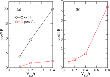
Figure 9: [Color Online] Coefficient $B$ of the exponential and power law fits (see text) of the RHC for (a) $n=0.5$ and (b) $n=1$, as a function of $V_{SO,x}/t$. Error bars are at least twice the size of the symbols used.

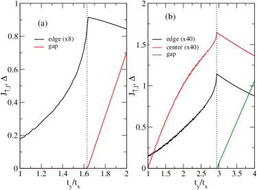
Figure 10: [Color Online] Spin-up currents on each chain as a function of $t_{y}/t_{x}$ for (a) 2-leg and (b) 4-leg rings, $L=800$, $V_{SO,x}/t_{x}=V_{SO,y}/t_{y}=1$, $t_{x}=1$, $n=0.5$.

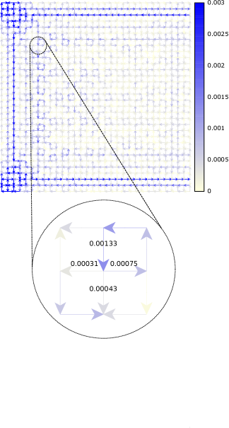
Figure 11: [Color Online] Spin-up currents on each nearest neighbor link, near the left end of the $256\times 32$ strip with OBC, $V_{SO}/t=0.8$ $n=0.5$. The colour of each arrow is proportional to the current strength, according to the included colour code. In the zoom, the currents on the links merging at the indicated site, are shown together with their absolute values.

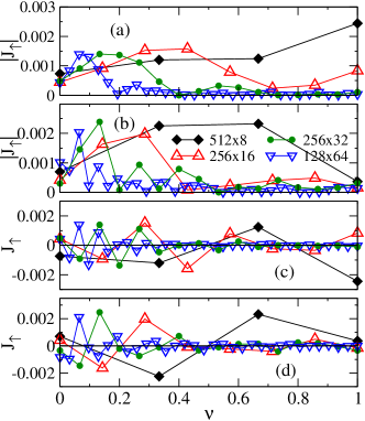
Figure 12: [Color Online] Absolute value of spin-up currents at the chain center as a function of the depth of the chain, (a) $V_{SO}/t=0.2$, (b) 0.8. Spin-up currents at the chain center, (c) $V_{SO}/t=0.2$, (d) 0.8. $L\times W$ indicated on the plot. Strips with OBC, $n=0.5$.

Let us emphasize that the behavior discussed in this Section occurs in the metallic phase. In Section IV.2, the effect of the Hubbard term and a possible Mott-Hubbard type of metal-insulator transition (MIT) will be considered. However, before leaving this Subsection, we can explore the effect of a MIT due to the opening of a band gap which may occur for sufficiently large ratio $t_{y}/t_{x}$, and at specific electron fillings. To this end, we should consider an spatially anisotropic extension of the Hamiltonian, where we keep the ratio $V_{SO,x}/t_{x}=V_{SO,y}/t_{y}=1$, and we do not use the normalization defined in Section II, but we used $t_{x}=1$ instead. In Fig. 10, a change of behavior in the Rashba helical currents is observed when a band gap opens in strips of widths $W=2$ and 4, at $n=0.5$. It is apparent that in the gaped region the RHC decrease approximately following a linear dependence, but clearly a more systematic research with more realistic band structures should be performed.

III.3 Results on open strips

We now turn to the geometry depicted in Fig. 1(b), with open boundary conditions in both directions. In this case, as shown in that Figure, the RHC would follow closed circuits. However, the currents on vertical segments would also present oscillatory behaviors similar to those shown previously for the currents on rings in the longitudinal direction. The result of the interference between horizontal and vertical oscillations leads to complex patterns, as the one illustrated in Fig. 11, that are little resembling the closed loops illustrated in Fig. 1(b), although some segments of closed loops are still visible near the edges.

One important difference between the full open strips considered in this Subsection, and rings, studied in the preceding one, is that spin-up and spin-down electron densities at each site, are no longer conserved separately, that is, the sum over the links connected to a given site of the hopping currents for each spin is no longer zero. This can be checked for example with the values of the currents in the zoom of Fig. 11. However, the Kirchhoff law for the total electron density at each site is still satisfied since on each link, $J_{\uparrow,x,y,\hat{\mu}}=-J_{\downarrow,x,y,\hat{\mu}}$, and the net SO current on each link is zero. It is interesting to notice, that in order to conserve the density of up electrons on each site, the currents $J^{\prime}_{SO,x,y,\hat{x}}$ defined after Eq. (4) must be nonzero in such a way that its sum over the links connected to a site must be equal to the corresponding sum of spin-up hopping currents. A similar conclusion can be reached for the sum of the spin-down currents and the other term of the SO currents, $J^{\prime\prime}_{SO,x,y,\hat{x}}$.

From the above discussion, to study the dependence of RHC on chains as a function of their distance to the edge, we have considered for simplicity the currents on the central link of these chains, that is $J_{\uparrow,L/2,\nu}$, where we have always adopted $L$ even. To reduce finite size effects, for each width we have taken the largest value of $L$ accessible to our computational facilities.

Figs. 12(a),(b) show results for the absolute value of $J_{\uparrow,L/2,\nu}$, at quarter filling, for $V_{SO}/t=0.2$ and 0.8, and for various strip widths. The overall behavior is similar to that found previously for rings for the same sets of parameters, that is, RHC is concentrated close to the edge for large $V_{SO}/t$ and $W$, while for small RSOC strength and widths, the overlapping of the tails of the decay from teh edges leads to RHC finite over the whole strip section. Results for $W=64$ are probably affected by finite size effects on the length $L$.

Similarly also to the case of rings, the oscillations actually stem from sign oscillations, as it can observed in Figs. 12(c),(d), for the same parameters as in Figs. 12(a),(b), respectively. Again, it seems that this oscillation has a wavenumber of $\pi$ at this density. Overall, the results for $J_{\uparrow,L/2,\nu}$ seem more erratic than the results for $J_{\uparrow,\nu}$ considered before for rings: although the later is a global quantity, the former is a local one.

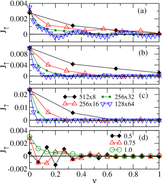
Figure 13: [Color Online] Spin-up current at the center of the chain as a function of the chain position, for (a) $V_{SO}/t=0.2$, (b) 0.4, (c) 0.8, (d) 0.8, and various values of the strip size, $L\times W$, as indicated on the plot, $n=1$. In (d) $J_{\uparrow}$ is shown for $V_{SO}/t=0.2$, and various values of the electron filling indicated on the plot, $256\times 32$. Strips with OBC.

In addition, a similar dependence of the results with the electron filling can be inferred by observing the results depicted in Fig. 13, corresponding to half-filling. Effects of $V_{SO}/t$ and $W$ are shown in Fig. 13(a)-(c), with an overall behavior similar to that shown before for rings, Fig. 8, that is, an apparent absence of oscillations except for the $128\times 64$, probably due to finite size effects. A somewhat more systematic study of the oscillations dependence on the electron filling is presented in Fig. 13(d), where results for $V_{SO}/t=0.2$, on the $256\times 32$ strip, for the fillings $n=0.5$, 0.75 and 1. For $n=0.75$, it seems that the oscillation has period four, consistent with a $4k_{F}$ value of $\pi/2$ in the first Brillouin zone.

To close this Subsection, let us emphasize that although it is not possible for open strips to reach the continuum limit as it was chieved in rings, the fact that one obtains essentially the same behavior indicates that finite size effects, and in lattice systems, the consequent discretized energy spectrum, are neligible.

IV Interacting case: currents due to external electromagnetic sources

Figure 14: [Color Online] Current of spin-up electrons as a function of the AB flux and various values of $U$ indicated on the plot, for $V_{SO}/t=0.6$, (a) edge chains $y=1$, $n=0.5$, (b) center chain, $n=0.5$, (c) edge chain $y=1$, $n=1$, (d) center chain, $n=1$. In (a) and (c), $J_{\uparrow,3}$ for $U=0$ was included. In (b) and (d), the spin-down current for $U=0$ has been added for comparison. Results obtained with VMC on the $16\times 3$ ring.

In this section, we will not only address the evolution of net carrier currents out of helical currents in Rashba metallic strips when external electromagnetic fields are applied, but also we will examine how electron correlations in the form of a Hubbard repulsion could affect those Rashba helical currents.

IV.1 Persistent currents

We will consider first how the RHC in the presence of persistent currents in rings will lead to net charge currents on each chain, both of the spin-conserving and the spin-flipping types, and to polarized currents, as well as spin accumulation. Persistent currents induced by an Aharonov-Bohm (AB) flux, are studied in this section by VMC, up to $U=8$. The value of each physical quantity obtained for a given $V_{SO}/t$ and $U$, density, and lattice size, is adopted as the average over the AB flux between 0 and $\pi$. Of course other criterions could be adopted, for example to take the maximum of the absolute value of each quantity on that interval of the AB flux.

The applied AB flux installs a net persistent hopping current, $J_{hop}/2=\sum_{l}J_{\uparrow,l,\hat{x}}=\sum_{l}J_{\downarrow,l,\hat{x}}\neq 0$, where the sum extends over all the chains of the strip. Since there is a net charge current along the longitudinal direction, it is well-known that a torque will appear on the spins making them rotate in the $(x,z)$ planeokudakimura , that is, there will be a net SO or spin-flipping current along the $x$-direction, $J_{SO}$. Then, the total current in the $x$-direction is $J_{tot}=J_{hop}+J_{SO}$

Let us start by discussing the case of three-chain rings. In Fig. 14, the evolution of RHC currents on each chain, $J_{\uparrow,y}$, with the AB flux, $\Phi$ is shown for $V_{SO}/t=0.6$, on the $16\times 3$ ring. In this, and in similar plots, we display properties as a function of the AB flux in the range $0\leq\Phi\leq\pi$, taking advantage of the symmetry $O(\Phi)=-O(2\pi-\Phi)$, where $O$ is any physical quantity. The relation involving the outer chains, $J_{\uparrow,1}=-J_{\uparrow,3}$, is broken as soon as $\Phi$ is different from zero, as illustrated in Fig. 14(a), for $n=0.5$ and $U=0$. However, the conditions $J_{\downarrow,1}=J_{\uparrow,3}$ and $J_{\uparrow,1}=J_{\downarrow,3}$, still hold for any $\Phi$. On the inner chain, it is observed, for $n=0.5$, (Fig. 14(b)) that $J_{\downarrow,2}=J_{\uparrow,2}$ for all $\Phi$. The same relations are present at half-filling, $n=1$, as shown in Fig. 14(c) for the outer chains, and in Fig. 14(d) for the inner chain. The dependence of $J_{\uparrow,y}$ with the Hubbard repulsion $U$ is also included in this plot. One should remember that in general VMC underestimates the effect of $U$. Nonetheless, it is quite apparent that the effects of $U$ at $n=1$ are stronger than at $n=0.5$. In fact, as we will see in the next Subsection, where the DMRG technique exactly treats the electron correlations, the model considered experiences a Mott-Hubbard type of metal-insulating transition, given by the vanishing of the total currents.

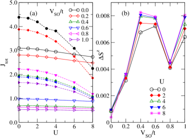
Figure 15: [Color Online] (a) Total current as a function of $U$ and for various $V_{SO}/t$ as indicated on the plot. Results for $n=0.5$ ($n=1$) are shown with empty (full) symbols. (b) Total spin accumulation as a function of $V_{SO}/t$ and various values of $U$ as indicated on the plot, $n=0.5$. Results obtained with VMC on the $16\times 3$ ring.

The results of a systematic study as a function of both $V_{SO}/t$ and $U$, are depicted in Fig. 15. In Fig. 15(a) it can be observed that the flux-averaged total currents decrease as a function of both $V_{SO}/t$ and $U$. For a fixed $V_{SO}/t$, this decreasing of $J_{tot}$ as a function of $U$ is much stronger for $n=1$ than for $n=0.5$, as expected on general grounds for the Hubbard repulsion. For both densities, and for any fixed value of $U$, the decrease of $J_{tot}$ with $V_{SO}/t$ is in general more important than the one due to $U$. In particular at $U=0$, this result for $W=3$ seems in contradiction with some suggestion in the literature that the longitudinal conductivity is independent of $V_{SO}/t$ and density.wong10 Further numerical support for the observed variation of $J_{tot}$ with $V_{SO}/t$ and density will be given in the next Subsection, and further discussion will be provided in the final Section. Results for the flux-averaged spin accumulation, is shown in Fig. 15(b). There is a general trend that $\Delta S^{z}$ reaches its maximum between $V_{SO}/t=0.4$ and 0.6 (the result for $V_{SO}/t=1.0$ is a finite size effect, since it is expected that $\Delta S^{z}$ vanishes as $V_{SO}/t\rightarrow\infty$), and more importantly, there is a general trend towards an enhancement of the spin accumulation with the Hubbard coupling $U$. Both features were already observed for the $W=2$ stripriera , and together with the results provided below for the $W=4$ strip, suggest that they could be valid for general strip widths $W$.

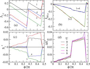
Figure 16: [Color Online] (a) Current of spin-up electrons, (b) SO current, and (c) total $S^{z}$, as a function of the AB flux $\Phi$, $U=0$. (d) Total spin accumulation as a function of the AB flux $\Phi$, and various values of $U$ indicated on the plot. Results obtained with VMC on the $16\times 4$ ring, $n=0.5$, $V_{SO}/t=0.6$.

In Fig. 16, we show the dependence of various quantities as a function of the AB flux $\Phi$ on the $16\times 4$ ring, $n=0.5$, and $V_{SO}/t=0.6$. In Fig. 16(a) the current of spin-up electrons is shown for each chain. Following the behavior above observed for the $W=3$ strip, the currents no longer satisfy the conditions $J_{\uparrow,y}=-J_{\uparrow,4-y+1}$ as soon as the AB flux is nonzero, but the relations $J_{\downarrow,y}=J_{\uparrow,4-y+1}$ still hold. The SO currents on each chain are shown in Fig. 16(b), where it can be verified the symmetry condition, $J_{so,y}=J_{so,4-y+1}$. The total $S^{z}(y)$ in each chain, which provides a measure of partial spin accumulation on each chain, is shown in Fig. 16(c). It should be noticed that the largest difference in $S^{z}(y)$ occurs between the symmetrical inner chains $y=2,3$. This largest contribution to the total spin accumulation from the inner chains occurs for all $V_{SO}/t$ (except the pathological case of $V_{SO}/t=0.8$) as it will be shown in Fig. 17(c). Finally, in Fig. 16(d) we show the total spin accumulation, defined as $\Delta S^{z}=S^{z}(1)+S^{z}(2)-(S^{z}(3)+S^{z}(4))$, confirming that its maximum value around $\Phi=0.4$ is mainly originated by the difference in $S^{z}(y)$ in the inner legs.

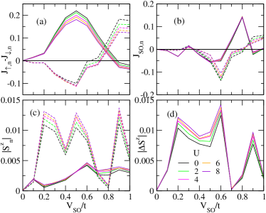
Figure 17: [Color Online] (a) Difference between spin-up currents (see text), (b) SO currents, and (c) absolute value of $\Delta S^{z}$, on external (full lines) and internal (dashed lines) chains, labelled on the plots, as a function of $V_{SO}/t$, and various values of $U$. (d) Total spin accumulation (in absolute value) for various values of $U$ indicated on the plot. Results obtained with VMC on the $16\times 4$ ring, $n=0.5$.

In Fig. 17(a), the flux-averaged spin-up electron currents on the external and internal legs of the four-chain ring are shown as a function of $V_{SO}/t$ and for the values of $U$ indicated on the plot. To be more precise, we plot the difference $J_{\uparrow,y}-J_{\uparrow,4-y+1}$, or equivalently, $J_{\uparrow,y}-J_{\downarrow,y}$, $y=1,2$. This average is equal to $J_{\uparrow,y}$ at $\Phi=0$. The behavior of the flux averaged differences have the same behavior of $J_{\uparrow,y}(\Phi=0)$, as it can be assessed by comparing it with Fig. 5(c) (differences between the results in both Figures are just finite size effects). It is interesting to notice that the current on the inner leg has the opposite sign of the current on the outer legs, and that both currents reach their maximum absolute value at $V_{SO}/t\sim 0.5$. After this point the inner current starts to increase becoming positive at $V_{SO}/t\sim 0.7$ while the outer current decreases. At $V_{SO}/t\sim 0.8$, the current in the inner leg becomes larger than the one of the outer leg.

In Fig. 17(b) SO currents in inner and outer legs are shown. In spite of an irregular behavior due to the finite size involved in the calculations, it can be seen observed that SO currents roughly follow the behavior of the up currents in the inner leg but their behavior is opposite for the outer legs. More relevant for spintronics applications is the behavior observed for the absolute value of $\Delta S^{z}_{n}=S^{z}_{n}-S^{z}_{4-n+1}$, shown in Fig. 17(c). It can be observed that $\Delta S^{z}_{2}$, corresponding to the inner legs, definitely dominates over $\Delta S^{z}_{2}$, corresponding to the outer legs, and determines the overall behavior of the resulting spin accumulation, $\Delta S^{z}$. The absolute value of this quantity is plotted in Fig. 17(d), and it can be observed that its maximum is obtained at intermediate values of $V_{SO}/t$, and also in agreement with previous calculations on the 2-leg ladderriera , it is enhanced by the Hubbard repulsion U.

IV.2 Voltage bias

In this subsection we present results obtained with DMRG on strips (or generalized ”ladders”) with two and three coupled chains (or ”legs”) with OBC in both directions. The purpose is to determine the time evolution of the Rashba helical currents following the sudden application of a bias voltage between both halves of the strip, as explained in Section II.

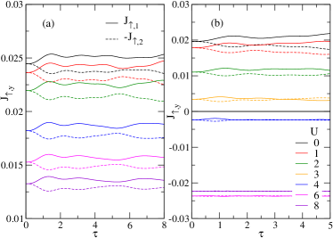
Figure 18: [Color Online] Time evolution of the currents of spin-up electrons on each chain of a 2-chain strip for various values of $U$ indicated on the plot, (a) $V_{SO}/t=0.6$, $n=0.5$, (b) $V_{SO}/t=0.4$, $n=1$. DMRG results for the $24\times 2$ strip with OBC. For the sake of clarity, $J_{\uparrow,2}=J_{\downarrow,1}$ (see text) has been inverted.

Similarly to the previous case, the applied voltage bias installs a net hopping current in the longitudinal $x$-direction, $J_{hop}$, together with a spin-flipping current, $J_{SO}$, and a total current, $J_{tot}=J_{hop}+J_{SO}$. This net SO current implies in turn that the two contributions $J^{\prime}_{SO,x,y,\hat{x}}$ and $J^{\prime\prime}_{SO,x,y,\hat{x}}$ will no longer cancel each other, and as a consequence, the relation on each link, $J_{\uparrow,x,y,\hat{\mu}}=-J_{\downarrow,x,y,\hat{\mu}}$ no longer holds. The antisymmetry of the system still implies that

$$J_{\uparrow,x,y,\hat{x}}=-J_{\downarrow,x,W-y+1,\hat{x}},$$ (9)

$y=1,\ldots,W$. Of course, no net SO current, which is a charge current, in the transversal direction will appear. A more subtle analysis would show the existence of transversal spin currentssinova04 , leading in turn to the spin accumulation that we will describe below.

As in Subsection III.3, the currents on each chain are measured at the center of each chain, $x=L/2$, and taking advantage of the condition Eq. (9), only the currents $J_{\uparrow,l,\hat{x}}$ will be shown in the figures below.

Let us start to examine the case of a strip with $W=2$, or ”two-leg ladder”. Although some results for the total hopping or spin-conserving, and SO or spin-flipping currents, were already reported,riera the main goal here is to explain their behavior in terms of the RHC studied in the previous Section, which are only slightly modified after applying the external voltage bias.

Fig. 18 shows the time-evolution of the up-spin electron currents on both chains of a $24\times 2$ strip, following the application of a voltage bias at time $\tau=0$. Figs. 18(a) and (b) correspond to electron fillings $n=0,5$ and $n=1$ respectively. For the sake of clarity, we have inverted one of them, $J_{\uparrow,2}$, since $J_{\uparrow,2}=-J_{\uparrow,1}=J_{\downarrow,1}=-J_{\downarrow,2}$ in the static case, that is, at the start of the time evolution. As it can be observed, as $\tau$ increases, both currents evolve following different oscillatory behaviors around their $\tau=0$ values. This difference leads to a nonzero total hopping current along each chain, $J_{\uparrow,1}+J_{\downarrow,1}$, and a net total current on the strip, as it will be further discussed below. During the whole time evolution the spin-down electron currents on each leg remain exactly equal to their spin-up counterpart on the opposite leg, that is $J_{\uparrow,2}=J_{\downarrow,1}$, $J_{\uparrow,1}=J_{\downarrow,2}$. Hence, on each chain there will appear a nonzero polarized current, $J_{pol,l}=J_{\uparrow,l}-J_{\downarrow,l}$, $l=1,2$ that cancel each other leading to an overall zero polarized hopping current along the strip.

For both densities considered, the effect of the Hubbard correlation is to suppress both the RHC currents as well as their difference. For $n=0.5$ (Fig. 18(a)) the system remains metallic for all $U$ considered, as it can be inferred from (Fig. 19(c)), and the RHC are smoothly decreasing while keeping their sign. On the other hand, at half-filling, (Fig. 18(b)) the RHC, as well as their differences, decrease more rapidly, and at $U\approx 3$ the RHC change their sign and they virtually cancel each other, leading to a vanishing overall current (Fig. 19(d)).

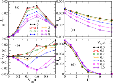
Figure 19: [Color Online] Current of spin-up electrons as a function of $V_{SO}/t$ and various values of $U$ indicated on the plot, for (a) $n=0.5$ and (b) $n=1$. Total current as a function of $U$ and various values of $V_{SO}/t$ indicated on the plot, for (c) $n=0.5$ and (d) $n=1$. Results obtained with DMRG on the $24\times 2$ strip with OBC.

The result of a systematic analysis of the behavior illustrated in Fig. 18 for the $24\times 2$ strip is presented in Fig. 19. At $n=0.5$, $U=0$, the current of spin-up electrons in leg ”1” at $\tau=0$ (Fig. 19(a)), which as discussed in the previous paragraph is approximately equal to $J_{pol,1}/2$, follows the general behavior illustrated in Fig. 5(a) for rings, with an approximate initial quadratic behavior as a function of $V_{SO}/t$, and becoming increasingly suppressed for $V_{SO}/t>0.6$. The effect of the Hubbard repulsion is to suppress these RHC, and this suppression is more pronounced near $V_{SO}/t=0.5$. The total currents for this filling, shown in Fig. 19(c) for various values of $V_{SO}/t$, are suppressed following the relation predicted for Luttinger liquids,kanefisher $J_{tot}(U)/J_{tot}(0)=K_{\rho}$ where $K_{\rho}$ is the one computed for Hubbard two-leg laddersorignac although the Rashba term could lead to corrections as observed in onedimensional systems. rashbaTL ; pletyukhov ; gritsev It is also worth to emphasize the striking similarity between the behavior of the RHC (Fig. 19(a)), as a function of $V_{SO}/t$, with the one of the spin accumulation as it can be seen in Fig. 4(c) of Ref. riera, . Of course, for $U=0$, this similarity could be eventually traced back to their common origin in the spin-Hall effect.sinova04 The fact that their behavior with increasing $U$ is the opposite is typical of Hubbard models, where magnetic orderings are in general opposed to transport.

Results at half-filling are strikingly different. The Rashba helical currents at $\tau=0$, shown in Fig. 19(b), are not only suppressed by $U$ but they also change their sign for large Hubbard repulsion. This behavior is somewhat erratic, particularly for $V_{SO}/t=0.4$. Notice that for large $U$, RHC become quite large in absolute value and their behavior is similar to the one for $n=0,5$. This behavior of the helical current is loosely correlated with the vanishing of $J_{tot}$ with $U$ (Fig. 19(d)), which indicates the Mott-Hubbard type of metal-insulator transition that is present in Hubbard two-leg ladders close to half-filling.noack

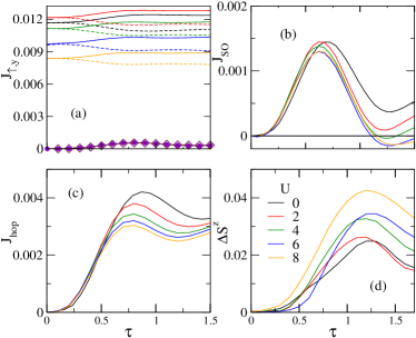
Figure 20: [Color Online] Time evolution of (a) $J_{\uparrow,1}$ (full lines) and $(-J_{\uparrow,3})$ (dashed lines), $J_{\uparrow,2}$, $J_{\downarrow,2}$ (dotted lines, only for $U=0$), (b) total SO current, (c) total hopping current (full lines) and total current (dashed lines), (d) total spin accumulation, for $V_{SO}/t=0.8$, various values of $U$ indicated on the plot, $n=0.5$. Results obtained with DMRG on the $16\times 3$ strip with OBC.

We try now to see if the previously discussed behaviors could be also found in wider strips by studying the strip with $W=3$. As it is well-known, numerical difficulties of applying DMRG to wider strips increase exponentially, hence most of the results shown below corresponds to a small strip, $8\times 3$, and finite size effects would be estimated by comparing with results for the $16\times 3$ strip, although in most cases we could only make qualitative statements.

Let start with the analysis of the time evolution of the RHC, computed on the $16\times 3$ strip, shown in Fig. 20(a). In this case, at $\tau=0$ the RHC in the external chains, $y=1$ and 3, have the same antisymmetric properties as the two chains in the $W=2$ strip, and these currents vanish on the central chain. As in the $W=2$ case, the voltage bias leads to oscillations of these currents around their $\tau=0$ values. Relatively small differences appearing between antisymmetric currents lead now to the appearance of a net charge hopping current as well as of a net charge SO current. The currents in the central chain, $J_{\uparrow,2}$ and $J_{\downarrow,2}$ evolve with $\tau$ around zero but having the same sign, that is, with net charge current and vanishing polarized current. The time evolution of RHC in the external chains, are similar to the ones observed for the $W=2$ chain, where not only a much stronger suppression with $U$ is observed, but also reversal of direction.

As discussed above, differences appearing between $J_{\sigma,y}$ currents, $\sigma=\uparrow,\downarrow$, $y=1,\ldots,3$, lead to net total SO currents, shown in Fig. 20(b), net total hopping currents, shown in Fig. 20(c) which summed give the total net current. Notice that $J_{hop}$ is, as before, about an order of magnitude smaller than the RHC, but still it is possible to reliably assign a plateau value to each of them although it is clearly seen that they are suppressed by the electron Hubbard $U$ term. The total SO currents are in turn an order of magnitude smaller than $J_{hop}$, and clearly, from Fig. 20(b), much more precision and consequent computer power would be required to assign to them an overall value. However, it seems that it can be observed a trend with $U$ of not only suppressing these SO currents but also to reversing its direction, which starts to occur just at the end of the time interval considered. This behavior is more clear for the smaller $8\times 3$ strip, where larger times can be achieved with our currrent computer facilites, and this direction reversal is consistent, although not as definite, with the behavior observed for the $W=2$ strip.riera In the same fashion, it is not reliable to assign a single value to the evolution of the spin accumulation, which is defined as $\Delta S^{z}=S^{z}_{1}-S^{z}_{3}$, where $S^{z}_{y}$ is the sum of all the average $z$-projection of the spin on each site on chain $y$. However, as it can be seen in Fig. 20(d), results point to a trend of enhancement of $\Delta$ with $U$, which again is consistent with the behavior observed for the $W=2$ strip. However, for $V_{SO}/t=0.4$ and 0.6, the behavior is not monotonic with $U$, and this is another indication that the $W=3$ strip may be not in the same class of the $W=2$ strip, which is not unexpected. Clearly, far more computational effort on the $W=3$ strip would be needed to set this question. Another interesting feature that can be observed in Fig. 20 is that $\Delta S^{z}$ reaches its maximum with a delay with respect to the time at which $J_{hop}$ and $J_{SO}$ reach their maximum. This delay is an indication of the presence of transversal spin currents appearing after the charge currents have been installed and leading to the spin accumulation, as expected in the SHE mechanism with open boundaries.

Figure 21: [Color Online] Current of spin-up electrons as a function of $V_{SO}/t$ and various values of $U$ indicated on the plot, for (a) $n=0.5$ and (b) $n=1$. Total current as a function of $U$ and various values of $V_{SO}/t$ indicated on the plot, for (c) $n=0.5$ and (d) $n=1$. Results obtained with DMRG on the $16\times 3$ strip ((a),(c)) and $8\times 3$ ((b),(d)) with OBC.

Finally, a more systematic dependence of the RHC as a function of $V_{SO}/t$ and $U$ is presented in Figs. 21(a) and (b), for $n=0.5$ and $n=1$, respectively. Although $J_{\uparrow,1}$ have nonmonotonic variations with $V_{SO}/t$, their variation with $U$ is noticeable weaker and smoother for $n=0.5$ than for $n=1$. Actually, for $n=1$, for most values of $V_{SO}/t$, $J_{\uparrow,1}$ changes its sign as $U$ is increased, similarly to the previous analyzed case of $W=2$ strips. Again, this behavior occurs while the total current, depicted in Fig. 21(d), goes to zero, indicating a Mott-Hubbard metal-insulation transition. On the other hand, the behavior of $J_{tot}$, for a given $V_{SO}/t$ decreases with $U$ following the general metallic behavior of quasi-onedimensional systems. We are not aware of Luttinger Liquid studies on the Hubbard model on $W=3$ strips, and consequent estimations of $K_{\rho}$.

V Conclusions

In this manuscript, we have described in the first place the spatial texture of Rashba helical currents in planar strips, as a function of various parameters, such as RSOC strength, strip width, electron filling, in the absence of external electromagnetic sources, and for the noninteracting case. By numerically solving the single particle Hamiltonian Eq. (1), we found that these RHC are mostly concentrated at the strip edges, but as the RSOC strength and/or the width are small enough, they appear as spread over the whole system. This is a different behavior to the one theoretically predicted for the helical edge currents, characteristic of the QSH, and topological insulators, as resulting for example from the Kane-Mele model. Certainly, this difference could be traced to the difference between the Haldane-like term for counter propagating spin up and down electrons, present in that model, which leads to the opening a gap in the energy spectrum, and hence to an insulator state in the bulk, and the Rashba SOC which favours the metallic state.

The results also suggest a periodicity of the sign oscillations of the RHC that could originate as Friedel oscillations induced by the edges, thus explaining its filling dependence. As mentioned in the Introduction, the natural source of these oscillations are local impurities, and in fact, the current inhomogeneities reported in Ref. bovenzi, could be of the same nature as the present RHC. It would be interesting to perform similar calculations on strips of the Kane-Mele model, for the sake of comparison.

In the second part of the present work, we consider the effects of charge currents induced by external electromagnetic sources, which could be relevant for actual spintronic devices. Our main results are that the RHC remain in the presence of such induced net currents, and their differences on each chain with respect to their stationary equilibrium values, help to explain how charge currents, both of the spin conserving or the spin flipping types, are distributed on each chain of the strip. These RHC also allow us to predict that on each chain there could be polarized charge currents, although the total current on the strip would be unpolarized.mhliu Since, as predicted by our handwaving model presented in Section III.1 in systems where Rashba and Dresselhaus SOC have equal strength, the RHC would not exist, and taking into account the relation between RHC and the net currents, it would be tempting to propose an explanation for the vanishing of optical conductivity at the persistent helix point.RDcond

In this study, we also include the presence of on-site electron correlations given by the Hubbard repulsion. In the context of topological insulators, it has been emphasized that the robustness of helical edge states with respect to interactions is a result of time-reversal symmetry, and in particular, the effect of a Hubbard term added to the Kane-Mele Hamiltonian has been thoroughly analyzed.laubach ; hohenadler In the model here considered, the RHC remain for finite values of $U$, although in the quasi-onedimensional metallic state, their are suppressed roughly following the prediction of Luttinger liquid theory. In fact, even if the system undergoes a Mott-Hubbard type of metal-insulator transition, as detected by the vanishing of the total current, the RHC are still present.

In principle, the Rashba helical currents would be as difficult to detect as the helical edge currents of the QSH. For the case of QSH, it has been shown that experimental evidence for helical edge currents can be achieved by multiterminal probes.buttiker ; roth2009 ; quay However, this scheme depends heavily on the strict edge character of QSH helical currents, and/or on the quantized nature of these currents. Clearly, a lot of ingenuity will be needed to adapt those experimental setups to measure the Rashba helical currents we observe in the present effort, and particularly the presence of polarized currents varying across the strip section. In addition, the study of a dissipationless character of the RHC is out of the scope of the present work. Notice that our model is dissipationless in the sense that it is not coupled to external degrees of freedom such as phonons.

Finally, we would like to emphasize apparent differences with some previous theoretical studies on this model. The band we consider is a cosine one, and we considered fillings $n\geq 0.5$, hence it is not simply reducible to a parabolic band, and, more importantly, the finite width of our system, and eventually also its finite length, sets a departure from previous studies on the infinite two-dimensional system. Certainly, finite size systems are per se relevant for nanoscale applications.

- (1) S. A. Wolf, D.D. Awschalom, R.A. Buhrman, J.M. Daughton, S. von Molnar, M.L. Roukes, A.Y. Chtchelkanova, D.M. Treger, Science 294, 1488 (2001).
- (2) G.A. Prinz, Science 282, 1660 (1998).
- (3) I. Zutic, J. Fabian, and S. Das Sarma, Rev. Mod. Phys. 76, 323, (2004).
- (4) D. Awschalom, Physics 2, 50 (2009).
- (5) J. Sinova, S. O. Valenzuela, J. Wunderlich, C. H. Back, and T. Jungwirth, Rev. Mod. Phys. 87, 1213
- (6) A. Hoffmann, IEEE Transactions on Magnetics 49, 5172 (2013).
- (7) E. I. Rashba, Sov. Phys. Solid State 2, 1109 (1960); Y. A. Bychkov and E. I. Rashba, JETP Lett. 39, 78 (1984).
- (8) R. Winkler, Spin-Orbit Coupling Effects in Two-Dimensional Electron and Hole Systems (Springer, New York, 2003).
- (9) M. I. Dyakonov and V. I. Perel, Sov. Phys. Solid State 13, 3023 (1972).
- (10) J. E. Hirsch, Phys. Rev. Lett. 83, 1834 (1999).
- (11) J. Sinova, D. Culcer, Q. Niu, N. A. Sinitsyn, T. Jungwirth, and A. H. MacDonald, Phys. Rev. Lett. 92, 126603 (2004).
- (12) S. Murakami, Phys. Rev. Lett. 97, 236805 (2006).
- (13) G. Vignale, J. Supercond. Nov. Magn. 23, 3 (2010).
- (14) B. K. Nikolić, S. Souma, L. P. Zârbo, and J. Sinova, Phys. Rev. Lett. 95, 046601 (2005).
- (15) A. G. Mal’shukov, L. Y. Wang, C. S. Chu, and K. A. Chao, Phys. Rev. Lett. 95, 146601 (2005).
- (16) D. Bercioux and P. Lucignano, Rep. Prog. Phys. 78, 106001 (2015).
- (17) S. I. Erlingsson, J. C. Egues, and D. Loss, Phys. Rev. B 82, 155456 (2010).
- (18) P. Wenk and S. Kettemann, Phys. Rev. B 83, 115301 (2011).
- (19) J. A. Riera, Phys. Rev. B 88, 045102 (2013).
- (20) F. Goth and F. F. Assaad, Phys. Rev. B 90, 195103 (2014).
- (21) H. Y. Hwang, Y. Iwasa, M. Kawasaki, B. Keimer, N. Nagaosa, and Y. Tokura, Nature Mater. 11, 103 (2012).
- (22) A. D. Caviglia, M. Gabay, S. Gariglio, N. Reyren, C. Cancellieri, and J.-M. Triscone , Phys. Rev. Lett. 104, 126803 (2010).
- (23) M. Ben Shalom, M. Sachs, D. Rakhmilevitch, A. Palevski, and Y. Dagan, Phys. Rev. Lett. 104, 126802 (2010).
- (24) Y. Kim, R. M. Lutchyn, and C. Nayak, Phys. Rev. B 87, 245121 (2013).
- (25) S. Caprara, F. Peronaci, and M. Grilli, Phys. Rev. Lett. 109, 196401 (2012).
- (26) C. Liu, S.-Y. Xu, N. Alidoust, T.-R. Chang, H. Lin, C. Dhital, S. Khadka, M. Neupane, I. Belopolski, G. Landolt, H.-T. Jeng, R. S. Markiewicz, J. H. Dil, A. Bansil, S. D. Wilson, and M. Z. Hasan, Phys. Rev. B 90, 045127 (2014).
- (27) S. Banerjee, O. Erten and M. Randeria, Nature Phys. 9, 626 (2013).
- (28) C. Sahin, G. Vignale, and M. E. Flatté, Phys. Rev. B 89, 155402 (2014).
- (29) G. Khalsa, B. Lee, and A. H. MacDonald, Phys. Rev. B 88 041302, (2013).
- (30) D. Bucheli, M. Grilli, F. Peronaci, G. Seibold, and S. Caprara, Phys. Rev. B 89 195448 (2014).
- (31) Z. Zhong, L. Si, Q. Zhang, W-G Yin, S. Yunoki and K. Held, Adv. Mater. Interfaces, 2, 5 (2015).
- (32) S. Murakami, N. Nagaosa, and S.-C. Zhang, Science 301, 1348 (2003).
- (33) B. A. Bernevig and S. C. Zhang, Phys. Rev. Lett. 96, 106802 (2006).
- (34) D. N. Sheng, Z. Y. Weng, L. Sheng, and F. D. M. Haldane, Phys. Rev. Lett. 97, 036808 (2006).
- (35) M. König, S. Wiedmann, C. Brüne, A. Roth, H. Buhmann, L. W. Molenkamp, X.-L. Qi, S.-C. Zhang, Science 318, 766 (2007).
- (36) C. L. Kane and E. J. Mele, Phys. Rev. Lett. 95, 146802 (2005).
- (37) T. Okuda and A. Kimura, J. Phys. Soc. Jpn. 82, 021002 (2013).
- (38) K. Nomura, J. Sinova, N. A. Sinitsyn, and A. H. MacDonald, Phys. Rev. B 72, 165316 (2005).
- (39) K. Nomura, J. Wunderlich, Jairo Sinova, B. Kaestner, A. H. MacDonald, and T. Jungwirth Phys. Rev. B 72, 245330 (2005).
- (40) M. Sakano, J. Miyawaki, A. Chainani, Y. Takata, T. Sonobe, T. Shimojima, M. Oura, S. Shin, M. S. Bahramy, R. Arita, N. Nagaosa, H. Murakawa, Y. Kaneko, Y. Tokura, K. Ishizaka, Phys. Rev. B 86, 085204 (2012).
- (41) T. P. Pareek and P. Bruno, Phys. Rev. B 65, 241305 (2002).
- (42) J. Zelezny, H. Gao, K. Vyborny, J. Zemen, J. Masek, A. Manchon, J. Wunderlich, J. Sinova, and T. Jungwirth, Phys. Rev. Lett. 113, 157201 (2014).
- (43) Y. Kato, R. C. Myers, A. C. Gossard, and D. D.Awschalom, Science 306, 1910 (2004).
- (44) S. D. Ganichev and L. E. and Golub, Phys. Status Solidi B 251 1801 (2014).
- (45) J. Splettstoesser, M. Governale, and U. Zulicke, Phys. Rev. B 68, 165341 (2003).
- (46) P. Michetti and P. Recher, Phys. Rev. B 83, 125420 (2011).
- (47) X. Q. Hong and J. E. Hirsch, Phys. Rev. B 41, 4410 (1990).
- (48) T. Giamarchi and C. Lhuillier, Phys. Rev. B 42, 10641 (1990).
- (49) U. Schollwöck, Rev. Mod. Phys. 77, 259 (2005).
- (50) A. E. Feiguin and S.R.White, Phys. Rev. B 72, 020404 (2005).
- (51) K. A. Al-Hassanieh, A. E. Feiguin, J. A. Riera, C. A. Busser, and E. Dagotto, Phys. Rev. B 73, 195304 (2006).
- (52) S. R. Manmana, S. Wessel, R. M. Noack, and A. Muramatsu, Phys. Rev. B 79, 155104 (2009).
- (53) P. Schmitteckert, Phys. Rev. B 70, 121302(R), (2004).
- (54) B. A. Bernevig, J. Orenstein, and S. C. Zhang, Phys. Rev. Lett. 97, 236601 (2006).
- (55) G. Dresselhaus, Phys. Rev. 100, 580 (1955).
- (56) N. Bovenzi, F. Finocchiaro, N. Scopigno, D. Bucheli, S. Caprara, G. Seibold and M. Grilli, J. Supercond. Nov. Magn. 28, 1273 (2015).
- (57) M. Z. Hasan, S.-Y. Xu and M. Neupane, arXiv:1406.1040.
- (58) Q. Sun, G.-B. Zhu, W.-M. Liu, A.-C. Ji, Phys. Rev. A 88, 063637 (2013).
- (59) Y. Baum, T. Posske, I. C. Fulga, B. Trauzettel, and A. Stern, Phys. Rev. Lett. 114, 136801 (2015).
- (60) M. Dzero, K. Sun, V. Galitski, and P. Coleman, Phys. Rev. Lett. 104, 106408 (2010).
- (61) B.-J. Yang and N. Nagaosa, Nature Communications 5, 4898 (2014).
- (62) G. A. Meza and J. A. Riera, Phys. Rev. B 90, 085107 (2014).
- (63) M. Laubach, J. Reuther, R. Thomale, and S. Rachel, Phys. Rev. B 90, 165136 (2014).
- (64) M. H. Liu, S.-H. Chen, and C.-R. Chang, Phys. Rev. B 78, 165316 (2008).
- (65) A. Wong and F. Mireles, Phys. Rev. B 81. 085304 (2010).
- (66) C. L. Kane and M. P. A. Fisher, Phys. Rev. B 46, 7268 (1992).
- (67) E. Orignac and T. Giamarchi, Phys. Rev. B 56, 7167 (1997).
- (68) W. Hausler, Phys. Rev. B 63, R121310 (2001).
- (69) M. Pletyukhov and V. Gritsev, Phys. Rev. B 70, 165316 (2004).
- (70) V. Gritsev, G. I. Japaridze, M. Pletyukhov, and D. Baeriswyl, Phys. Rev. Lett. 94, 137207 (2005).
- (71) R. M. Noack, S. R. White, and D. J. Scalapino, Physica C 270, 281 (1996).
- (72) Z. Li, F. Marsiglio, and J. P. Carbotte, Sci. Rep. 3, 2828 (2013).
- (73) M. Hohenadler and F. F. Assaad, Phys. Rev. B 90, 245148 (2014).
- (74) M. Buttiker, Science 325, 278 (2009).
- (75) A. Roth, C. Brüne, H. Buhmann, L. W. Molenkamp, J, Maciejko, X.-L. Qi, S.-C. Zhang, Science 325, 294 (2009).
- (76) C. H. L. Quay, T. L. Hughes, J. A. Sulpizio, L. N. Pfeiffer, K. W. Baldwin, K. W. West, D. Goldhaber-Gordon and R. de Picciotto, Nature Physics 6, 336 (2010).