Node-By-Node Greedy Deep Learning for Interpretable Features

Abstract

Multilayer networks have seen a resurgence under the umbrella of deep learning. Current deep learning algorithms train the layers of the network sequentially, improving algorithmic performance as well as providing some regularization. We present a new training algorithm for deep networks which trains each node in the network sequentially. Our algorithm is orders of magnitude faster, creates more interpretable internal representations at the node level, while not sacrificing on the ultimate out-of-sample performance.

1 Introduction

Multilayer neural networks have gone through ups and downs since their arrival in (Rosenblatt, 1958; Widrow, 1960; Hoff Jr, 1962). The resurgence in “deep” networks is largely due to the efficient greedy layer by layer algorithms for training, that create meaningful hierarchical representations of the data. Particularly in the era of “big data” from diverse applications, efficient training to create data representations that provide insight into the complex features captured by the neurons are important. We explore these two dimensions of training a deep network. Assume a standard machine learning from data setup (Abu-Mostafa et al., 2012), with $N$ datapoints $({{\mathbf{x}}}_{1},y_{1}),\ldots,({{\mathbf{x}}}_{N},y_{N})$; ${{\mathbf{x}}}_{n}\in\mathbb{R}^{d}$ and $y_{n}\in\{0,1,\ldots,c-1\}$ (multi-class setting).

Deep Network

We refer to Abu-Mostafa et al. (2012, Chapter 7) for the basics of multilayer networks, including notation which we very quickly summarize here. On the right, we show a feedforward network architecture. Such a network is “deep” because it has many ($\gg 2$) layers. We assume that a network architecture has been fixed. The network implements a function whereby in each layer ($\ell$), the output of the previous layer ($\ell-1$) is transformed into the output of the layer $\ell$ until one reaches the final layer on top, which is the output of the network. The function implemented by layer $\ell$ is

$${{\mathbf{x}}}^{(\ell)}=\tanh({{\mathrm{W}}}^{(\ell)}{{\mathbf{x}}}^{(\ell-1)}),$$

where ${{\mathbf{x}}}^{(\ell)}$ is the output of layer $\ell$, and the weight-matrix ${{\mathrm{W}}}^{(\ell)}$ (of appropriate dimensions to map a vector from layer $\ell-1$ to a vector in $\ell$) are parameters to be learned from data. The training phase uses the data to identify all the parameters $\{{{\mathrm{W}}}^{(1)},{{\mathrm{W}}}^{(2)},\ldots,{{\mathrm{W}}}^{(L)}\}$ of the deep network.

Backpropagation which trains all the weights simultaneously, allowing for maximum flexibility, was the popular approach to training a deep network (Rumelhart et al., 1986). The current approach is layer-by-layer: train the first layer weights ${{\mathrm{W}}}^{(1)}$; then train the second layer weights ${{\mathrm{W}}}^{(2)}$, keeping the first layer weights fixed; and so on until all the weights are learned. In practice, once all the weights have been learned in the greedy-layer-by-layer manner (often referred to as pre-training), the best results are obtained by fine tuning all the weights using a few iterations of backpropagation (Figure 1).

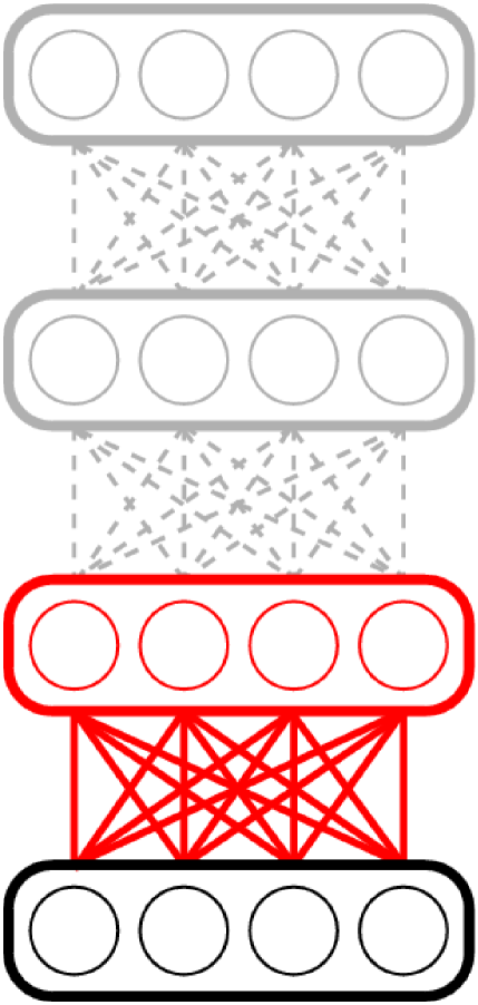
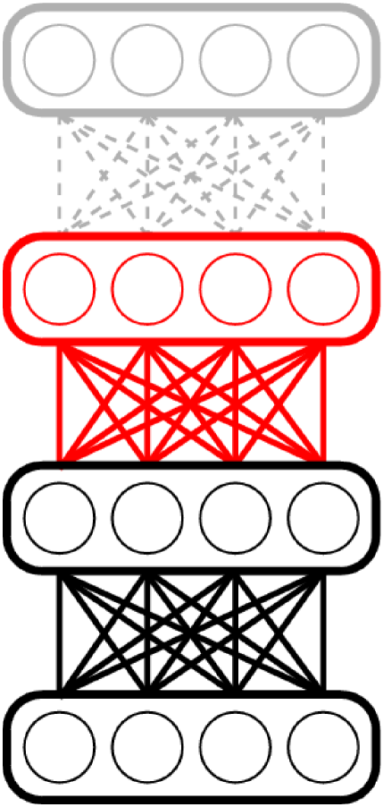
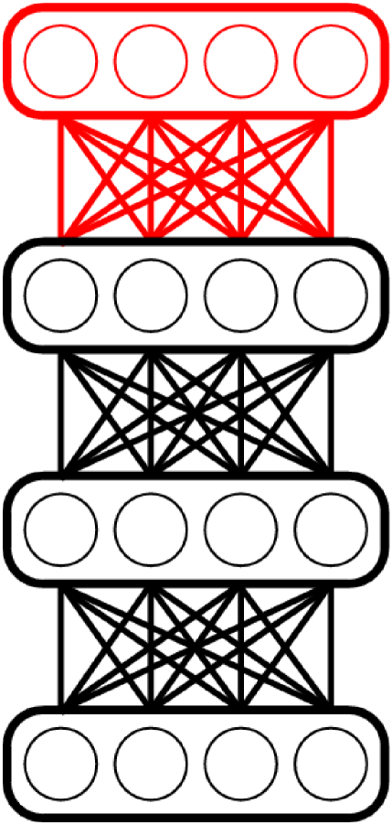
Learn ${{\mathrm{W}}}^{(1)}$ Learn ${{\mathrm{W}}}^{(2)}$ Learn ${{\mathrm{W}}}^{(3)}$ Fine tuning

Figure 1: Layer-by-layer greedy deep learning algorithm.

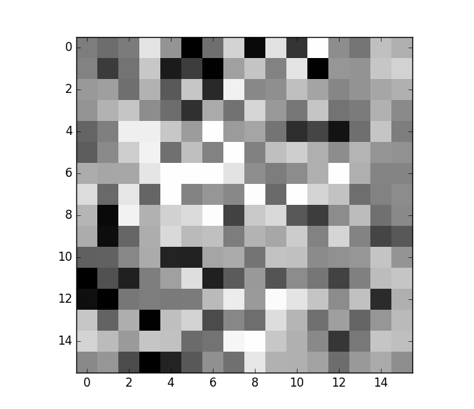
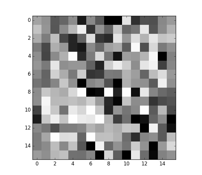
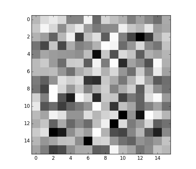
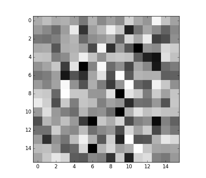
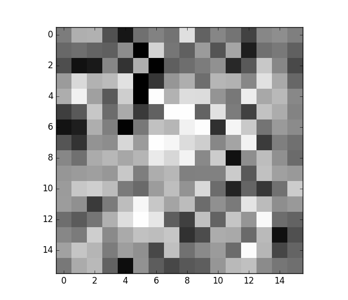
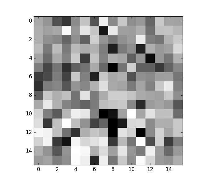
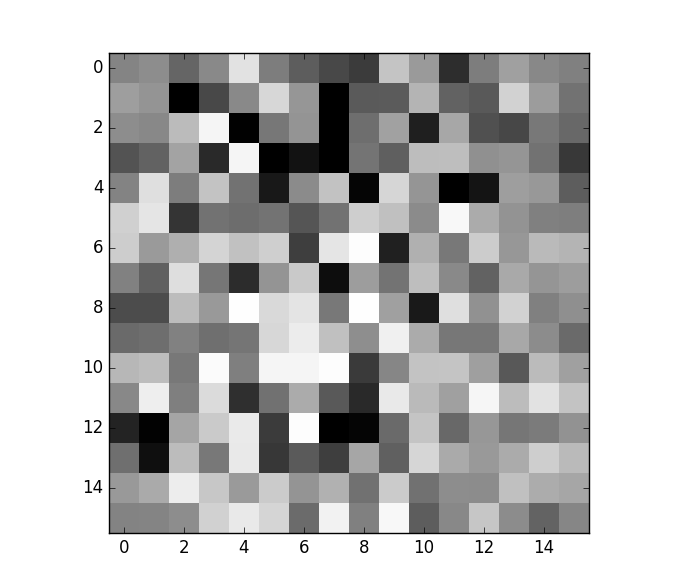
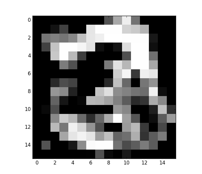
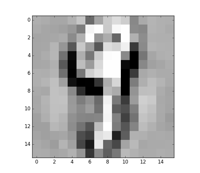
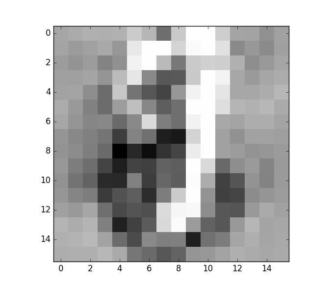
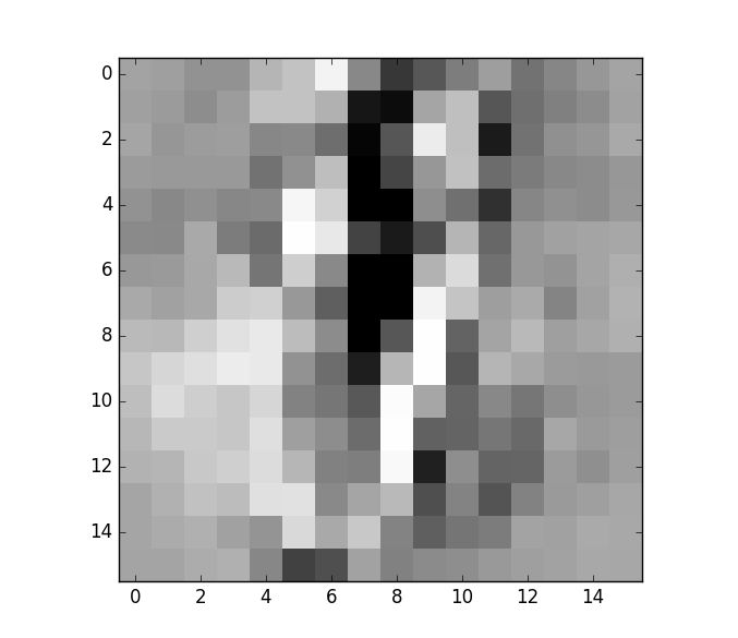
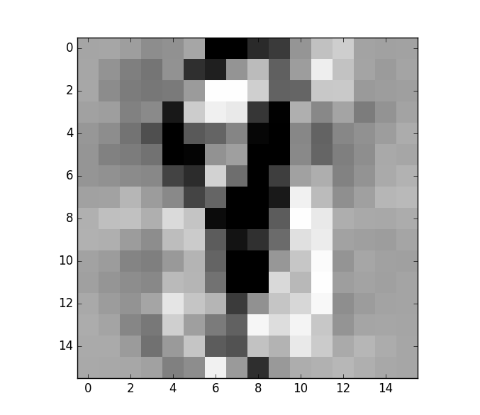
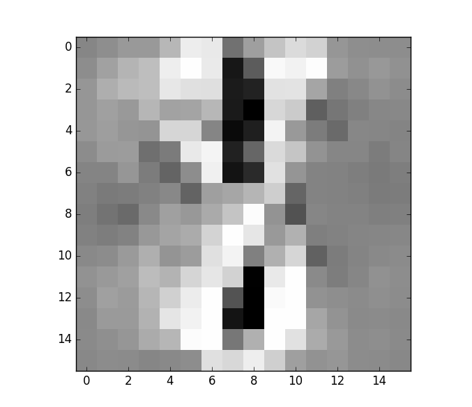
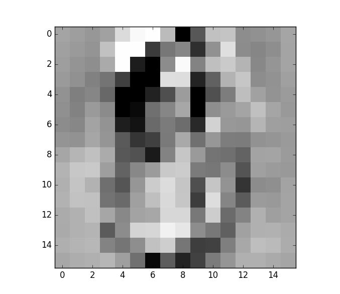
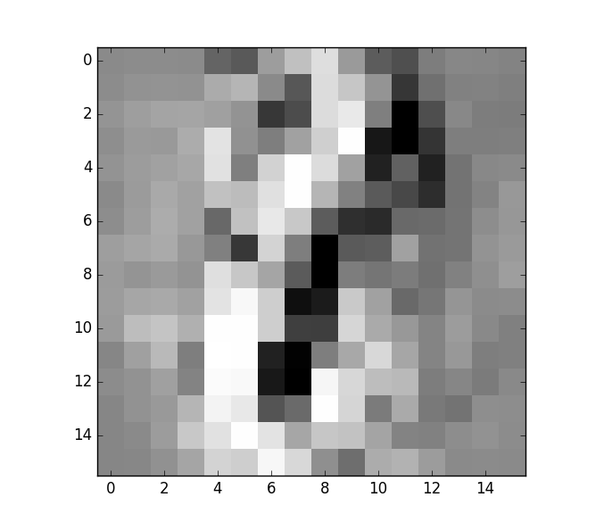
Layer-by-Layer Unsupervised Autoencoder	Our Greedy Node-by-Bode Unsupervised Algorithm (GN)

Figure 2: Features of nine nodes in the first internal layer for unsupervised pre-training.

How one should train the internal layers? The two popular approaches are: (1) Each layer is an unsupervised nonlinear auto-encoder (Cottrell & Munro, 1988; Bengio et al., 2007); this approach is appealing to build meaningful hierarchical representations of the data in the internal layers. (2) Each layer is a supervised encoder; this approach primarly targets performance. Deep learning enjoys success in several applications and hence considerable effort has been expended in optimizing the pre-training. The two main considerations are:

1. Pre-training time and training/test performance of the final solution. The greedy layer-by-layer pre-training is significantly more efficient than full backpropagation, and appears to be better at avoiding bad local minima (Erhan et al., 2010). Our algorithms will show an order of magnitude speed gain over greedy layer-by-layer pre-training.

2. Interpretability of the feature representations in the internal layers. We use the USPS digits data (10 classes) as a strawman benchmark to illustrate our approach. The weights going into each node of the first layer identify the pixels contributing to the “high-level” feature represented by that hidden node. Figure 2 compares our features with the layer-by-layer features in the unsupervised setting, and Figure 4 compares the features in the supervised setting. The layer-by-layer features do not capture the essence of the digits as do our features. This has to do with the simultaneous training of all the hidden nodes in the layer. Our approach can be viewed as a nonlinear extension of PCA, which ”greedily” constructs each linear features. (In the supplementary material, we show the features captured by linear PCA; they are comparable to our features.)

Greedy Node-by-Node Pre-Training.

The thrust of our approach is to learn the weights into each node in a sequential greedy manner: greedy-by-node (GN) for the unsupervised setting and greedy-by-class-by-node (GCN) for the supervised setting. Figure 3 illustrates the first 5 steps for a network.

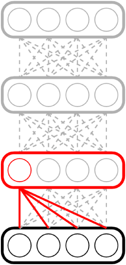
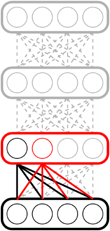
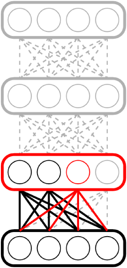
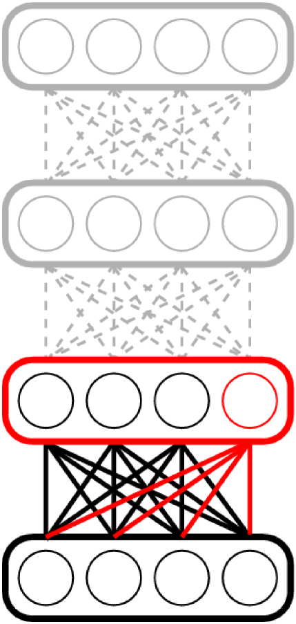
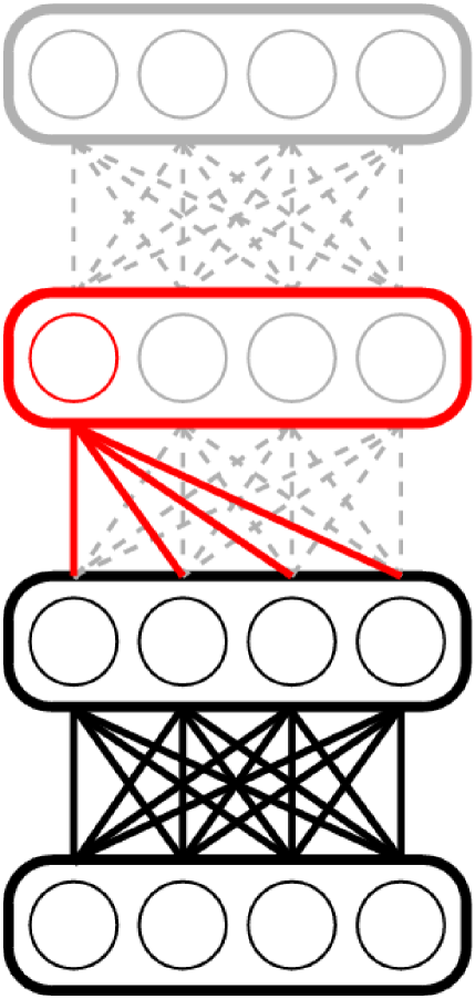
${{\mathrm{W}}}^{(1)}_{1}$	${{\mathrm{W}}}^{(1)}_{2}$	${{\mathrm{W}}}^{(1)}_{3}$	${{\mathrm{W}}}^{(1)}_{4}$	${{\mathrm{W}}}^{(2)}_{1}$

Figure 3: Node-by-node greedy deep learning algorithm. In each step the weights feeding into one node are learned (red).

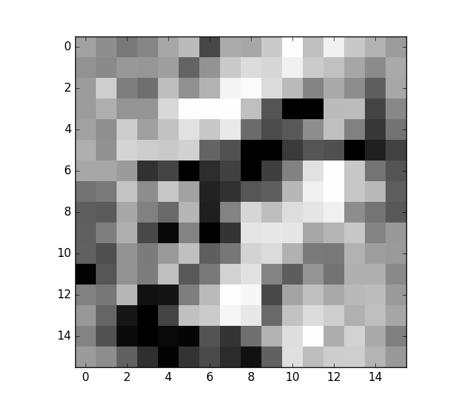
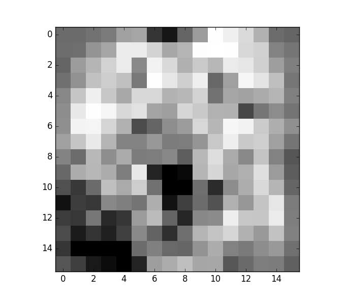
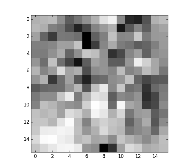
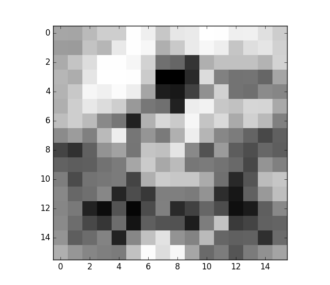
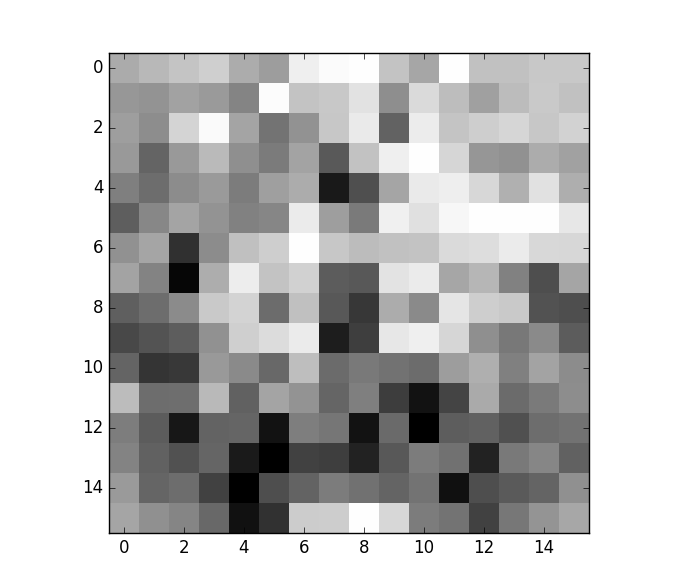
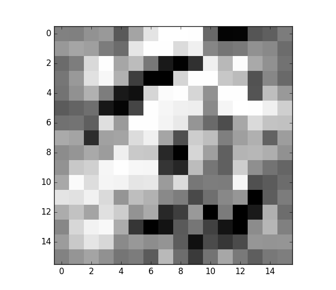
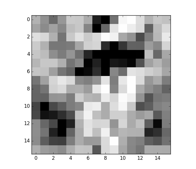
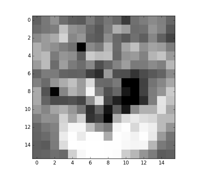
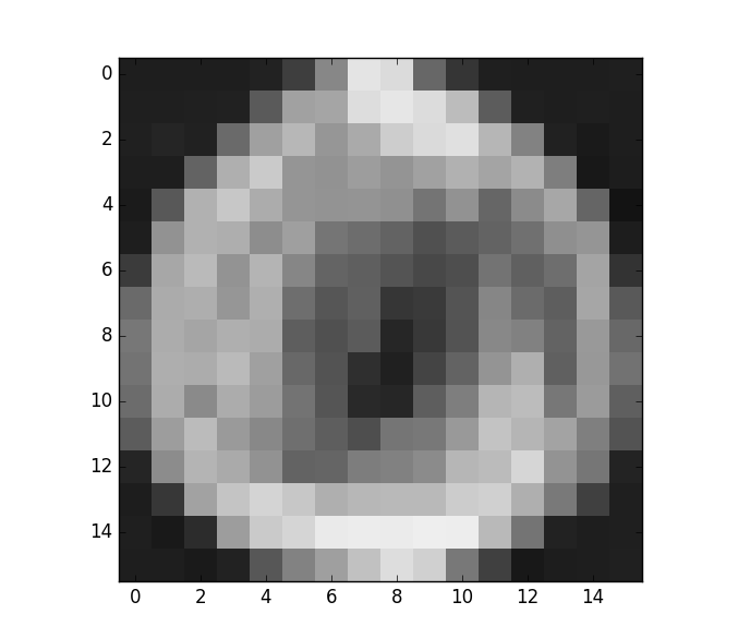
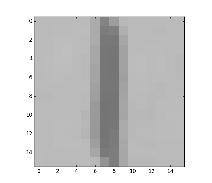
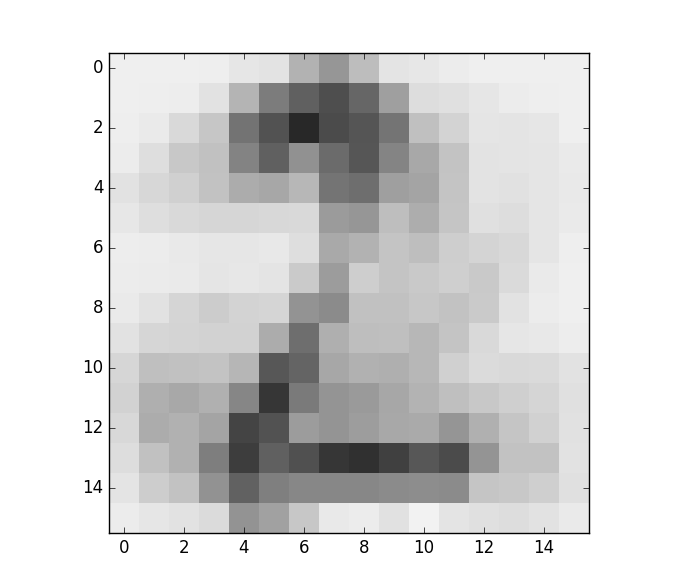
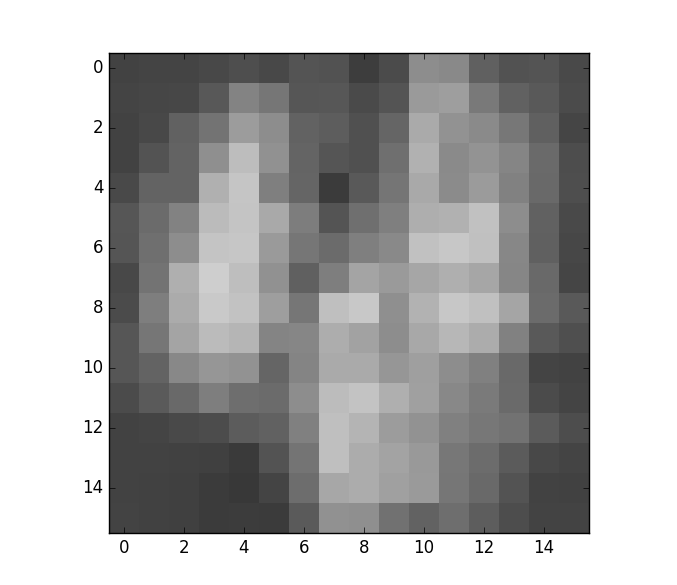
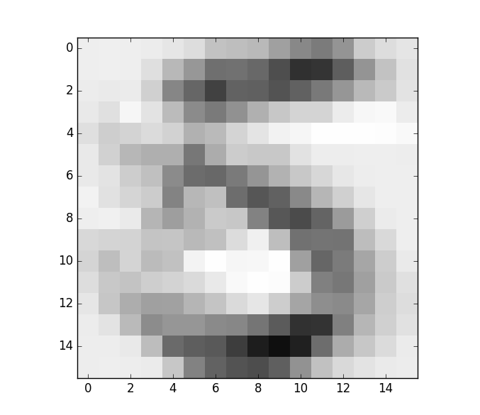
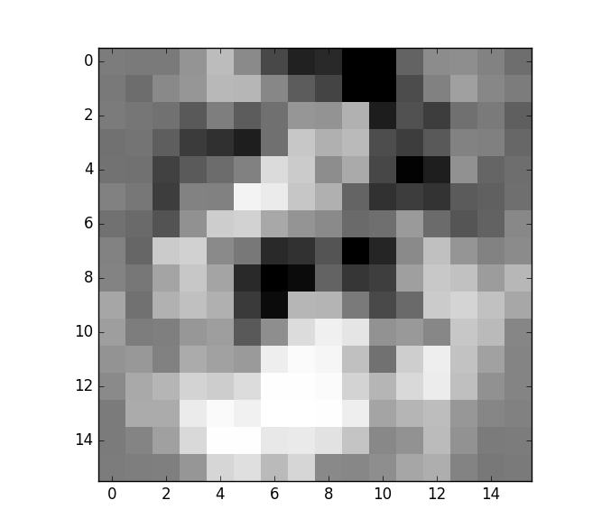
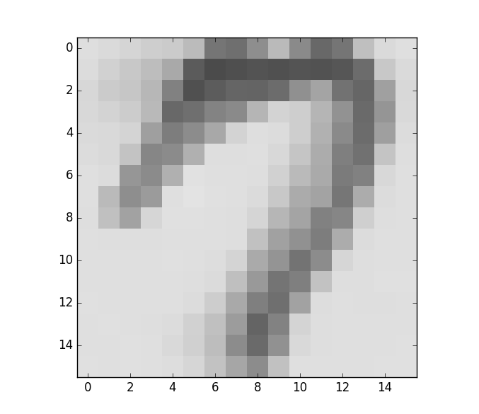
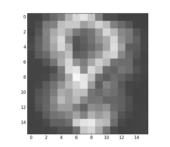
Layer-by-Layer Supervised Encoder	Our Greedy Node-by-Node Supervised Algorithm (GCN)

Figure 4: Features of nine nodes in the first internal layer for supervised pre-training.

Our approach mimics a human who hardly builds all features at once from all objects. Instead, features are built sequentially, while processing the data. Our algorithm learns one feature at a time, using a part of the data to learn each feature. Our contributions are

1. The specific algorithm to train each internal node.

2. How to select the training data for each internal node.

We do not improve the accuracy of deep learning. Rather, we improve efficiency and the interpretability of features, while maintaining accuracy. A standard deep learning algorithm uses every data point to process every weight in the network. Our algorithm uses only a subset of the data to process a particular weight. By training each node using ”relevant” data, our algorithm produces more interpretable features. Our algorithm gets more intuitive features, in the unsupervised and supervised setting (Figures 2 and 4).

Related Work.

To help motivate our approach, it helps to start back at the very beginning of neural networks, with Rosenblatt (1958) and Widrow (1960). They introduced the adaline, the adaptive linear (hard threshold element), and the combination of multiple elements came in Hoff Jr (1962), the madaline (the precursor to the multilayer perceptron). Things cooled off a little because fitting data with multiple hard threshold elements was a combinatorial nightmare. There is no doubt softening the hard threshold to a sigmoid and the arrival of a new efficient training algorithm, backpropagation (Rumelhart et al., 1986), was a huge part of the resurgence of neural networks in the 1980s/1990s. But, again, neural networks receded, taking a back seat to modern techniques like the support vector machine (Vapnik, 2000). In part, this was due to the facts that multilayer feedforward networks were still hard to train iteratively due to convergence issues and multiple local minima (Gori & Tesi, 1992; Fukumizu & Amari, 2000), are extremely powerful (Hornik et al., 1989) and easy to overfit to data. For these reasons, and despite the complexity theoretic advantages of deep networks (see for example the short discussion in (Bengio et al., 2007)), application of neural networks was limited mostly to shallow two layer networks. Multi-layer (deep) neural networks are back in the guise of deep learning/deep networks, and again because of a leap in the methods used to train the network (Hinton et al., 2006). In a nutshell, rather that address the full problem of learning the weights in the network all at once, train each layer of the network sequentially. In so doing, training becomes manageable (Hinton et al., 2006; Bengio et al., 2007), the local minima problem when training a single layer is significantly diminished as compared to the whole network and the restriction to layer by layer learning reigns in the power of the network, helping with regularizing it(Erhan et al., 2010). A side benefit has also emerged, which is that each layer successively has the potential to learn hierarchical representations (Erhan et al., 2010; Lee et al., 2009a). As a result of these algorithmic advances, deep networks have found a host of modern applications, ranging from sentiment classification (Glorot et al., 2011), to audio (Lee et al., 2009b), to signal and information processing (Yu & Deng, 2011), to speech (Deng et al., 2013), and even to the unsupervised and transfer settings (Bengio, 2012). Optimization of such deep networks is also an active area, for example (Ngiam et al., 2011; Martens, 2010).

Most work has focused on better representations of the input data. Besides the original deep belief network (Hinton et al., 2006) and autoencoder (Bengio et al., 2007), the stacked denoising autoencoder (Vincent et al., 2010, 2008) has been widely used as a variant to the classic autoencoder, where corrupted data is used in pre-training. Sparse encoding (Boureau et al., 2008; Poultney et al., 2006) has also been used to prevent the system from activating the same subset of nodes constantly (Poultney et al., 2006). This approach has been shown capable of learning local and meaningful features, however the efficiency is worse. For images, convolutional neural networks (LeCun & Bengio, 1995) and the deep convolutional neural network  (Krizhevsky et al., 2012) are widely used, however the computation cost is significantly more, and the feature learning is based on the local filter defined by the modeler. Our methods apply to a general deep network. Our algorithms can be roughly seen as simultaneously clustering the data while extracting the features. Deep networks have been used for unsupervised clustering (Chen, 2015) and clustering has been used in classic deep networks by Weston et al. (2012) which are targeted for semi-supervised learning. Using clusters from $K$-means to train a deep network was reported (Faraoun & Boukelif, 2006), which improves the training speed while ignoring some data - not recommended in the supervised setting with scarce data. Pre-clustering may have efficiency-advantages in large-scale systems, but it may not be an effective way to learn good representations (Coates & Ng, 2012).

In this paper, we are proposing a new algorithmic enhancement to the deep network which is to consider each node separately. It not only explicitly achieves the sparsity of node activation but also requires much shorter computation time. We have found no such approaches in the literature.

2 Greedy Node-by-Node Deep Learning

The basic step for pre-training is to train a two layer network. The network is trained to reproduce the input (unsupervised) or the final target (supervised). The two algorithms are very similar in structure. For concreteness, we describe unsupervised pre-training (auto-encoding).

In a classic auto-encoder with one hidden layer using stochastic gradient descent (SGD), the number of operations (fundamental arithmetic operations) $p$ for one training example is:

$$\begin{array}[]{rclcl}p&=&(2d_{1}d_{2}+d_{1}+2d_{2})&+&(3d_{1}d_{2}+2d_{1}+3d_{2})\\ &&\text{\small(Forward Propagation)}&&\text{\small(Backpropagation)}\\ &=&5d_{1}d_{2}+3d_{1}+5d_{2},\end{array}$$ (1)

where $d_{1}$ is the dimension of the input layer, ($d_{1}+1$ including the bias) and $d_{2}$ is the dimension of the second layer. Forward propagation computes the output and backpropagation computes the gradient of the loss w.r.t. the weights (see Abu-Mostafa et al. (2012, Chapter 7)). We use the Euclidean distance between the reconstructed input $\hat{{\mathbf{x}}}$ and the original input ${{\mathbf{x}}}$ (auto-encoder target) as loss,

$$\text{loss}={\|{{\mathbf{x}}}-\hat{{\mathbf{x}}}\|}^{2}.$$

For $N$ training example and $E$ epochs of SGD, the total running time is $O(NpE)=O(NEd_{1}d_{2})$.

In our algorithm, the basic step is also to train a 2-layer network. However, we train each node sequentially in a greedy fashion as illustrated in Figure 5. The red (middle) layer is being trained (it has dimension $d_{2}$). The inputs come from the outputs of the previous layer, having dimension $d_{1}$. The output-dimension is also $d_{1}$ (auto-encoder). We use linear output-nodes and SGD optimizing the auto-encoder (the algorithm is easy to adapt to sigmoid output-nodes).

Figure 5: Greedy training of a 2-layer network

The standard layer-by-layer algorithm trains all the weights at the same time, using the whole data set. We are going to use a fraction of the data to learn one feature at a time; different features are learned on different data. So, the training of each layer is done in multiple stages. At each stage, we only update the weights corresponding to one node. After all the features are obtained (all the weights learned) for a layer, a forward propagation with all data computes the outputs of the layer, for use in training the next layer (as in standard pre-training). To make this greedy learning algorithm work, we must address three questions:

1. How to learn features sequentially?

2. How to distribute the training data into each node?

3. How to obtain non-overlapping features?

Let us address the question 1, assuming we have already created $d_{2}$ subsets of the data of size $K$, $S_{1},\ldots,S_{d_{2}}$. These subsets need not be disjoint, but our discussion is for the case of disjoint subsets, so $Kd_{2}=N$. If each node is fed a random subset of $K$ data points, then each node will be roughly learning the same feature, that is close to the top principle component. We will address this issue is questions 2 and 3 which encourage learning different features by implementing a form of orthogonality and using different data for each node.

A simple idea which works but is inefficient: use data $S_{i}$ to train the weights into hidden node $i$ (assuming weights into nodes $1,\ldots,(i-1)$ have been trained). The situation is illustrated in Figure 5. The weights into and out of node 1 are fixed (black). Node 2 is being trained (the red weights into and out of node 2). We use data $S_{2}$ to train these red weights, so we forward propagate the data through both nodes, but we only need to backpropagate through the red nodes. Effectively, we are forward propagating through a network of $i$ hidden nodes, but we have $K$ data points, so the run-time is of just the forward propagations is

$$\sum_{i=1}^{d_{2}}O(KEd_{1}i)=O(KEd_{1}d_{2}^{2}).$$

Since $d_{2}$ could be large, it is inefficient to have a quadratic in $d_{2}$ run-time. There is a simple fix which relies on the fact that the outputs of the hidden layer are linearly summed before feeding into the output layer. This means that after the weights for node 1 are learned (and fixed), one can do a single forward propagation of all the data once through this node and store a running sum of the signal being fed into each output-layer node, which is the sunning contribution from all previously trained nodes in the hidden layer. This restores the linear dependence on $d_{2}$ as in equation (1).

Distributing data into nodes: We now address the 2nd question. We propose two methods corresponding to the two new algorithms GN and GCN. There are many ways to extend these two basic methods, so we present only the rudimentary forms. Each node $i$ is trained on subset $S_{i}$. In the unsupervised setting (GN), we train node 1 to learn a “global feature”, and use this single global feature to reconstruct all the data. The reconstruction error from this single feature is then used to rank the data. A small reconstruction error means the data point is captured well by the current feature. Large reconstruction errors mean a new feature is needed for those data. So the reconstruction error can be used as an approximate proxy for partitioning the data into different features: data with drastically different reconstruction error correspond to different features, so that data will be used to train its own feature. After sorting the data according to reconstruction error, the first $N/(d_{2}-1)$ will be used to train node $2$, the next $N/(d_{2}-1)$ to train node $3$ and so on up to node $d_{2}$. One may do more sophisticated things, like cluster the reconstruction errors into $d_{2}-1$ disjoint clusters and use those clusters as the subsets $S_{2},\ldots,S_{d_{2}}$. We present the simplest approach.

In the supervised setting (GCN), the only change is to modify the distribution of the data into nodes using the class labels. If there are $c$ classes, then $d_{2}/c$ of the nodes will be dedicated to each class, and the data points in each class are distributed evenly among the nodes dedicated to that class.

Ensuring Non-Overlapping Features. If every node is trained independently on all or a random sample of the data, then each node will learn more-or-less the same feature. Our method of distributing the data among the nodes to some extent breaks this tie. We also introduce an explicit coordination mechanism between the nodes which we call the amnesia factor – when training the next node, how much of the prior training is “forgotten”. Recall that from the previous $i-1$ (already trained) nodes, we store the running contribution to the output. SGD is applied based on the distance between the input and the sum of the current output and running stored value from the previous $i-1$ nodes. The running stored value can be viewed as a constraint on the training of node $i$, forcing the newly learned feature to be ”orthogonal” to the previous ones. This is because the previous features are encoded in the running stored value. The current value produced by node $i$ will try to contribute additional information toward reconstruct the data in $S_{i}$. Since, in our algorithms, the weights from the previous nodes have been learned and fixed, due to their optimization, it may prematurely saturate the output layer and make the new $i$th node redundant. The amnesia factor gives the ability to add just the right amount of coordination between the training of node $i$ and the nodes that have already been trained, leading to stability of the features while at the same time maintaining the ability to get non-redundant features. Our implementation of amnesia is simple. The output value, $O_{B}$, used for backpropagation to train the weights into node $i$ are the stored (already learned) running output, $O_{(1:i-1)}$, scaled by the amnesia factor plus the output from the currently being trained node $O_{i}$,

$$O_{B}=A\cdot O_{(1:i-1)}+O_{i}.$$

The amnesia factor controls how “orthogonal” each successive feature will be to the previously trained features. A higher amnesia factor results in strongly coupled features that are more orthogonal. A zero amnesia factor means independent training of the nodes which is likely to result in redundant features. Here is a high-level summary of the full algorithm. Detailed pseudo-code is presented in the supplementary materials.

1:  Distribute the data into subsets $S_{1},\ldots,S_{d_{2}}$

2:  Train hidden node $i$ on data $S_{i}$ using amnesia factor $A$

3:  Perform one forward propagation with $S_{i}$ on nodes $1,\ldots,i$ after training, and add the output values to the running output value.

Theorem 1

GN and GCN run in $O(NEd_{1}+Nd_{1}d_{2})$ time.

(The detailed derivation of the running time is in the supplementary materials.) The run-time of the classic deep-network algorithm is $O(NEd_{1}d_{2})$. As $d_{2}$ and $E$ (the number of iterations of SGD on each data point) increase, the efficiency gain increases, and can be orders of magnitude.

3 Results and Discussion

We use a variety of data sets to compare our new algorithms GN (unsupervised) and GCN (supervised) against some standard deep-network training algorithms. Our aim is to demonstrate that

• Features from GN and GCN are more interpretable.

• The classification performance of our algorithms is comparable to layer-by-layer training, despite being orders of magnitude more efficient.

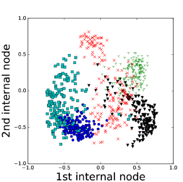
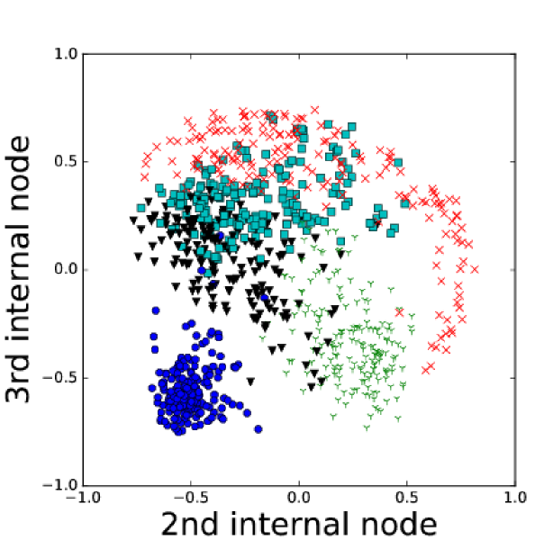
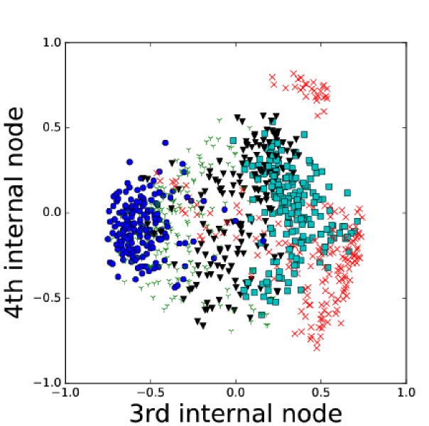
AE

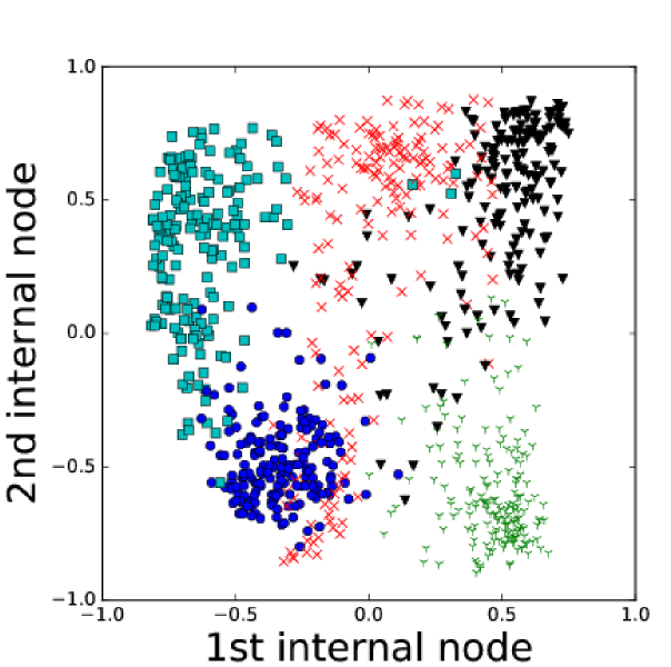
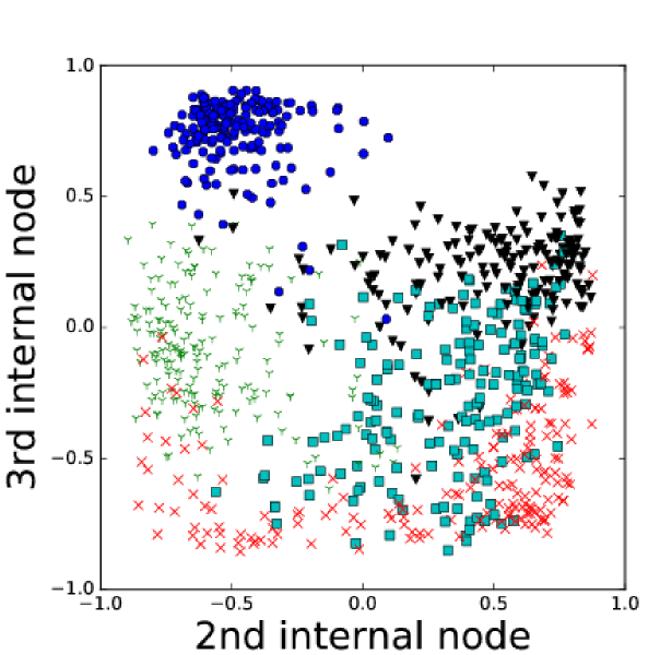
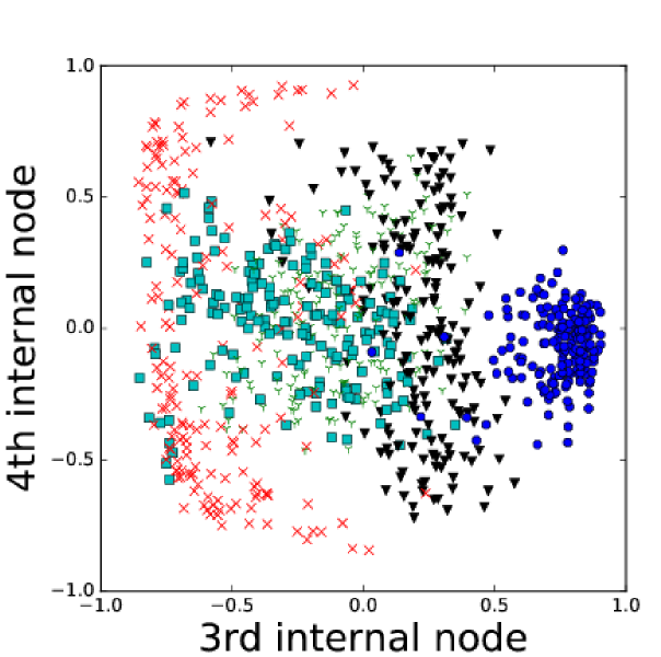
GN

Figure 6: Outcomes of four inner nodes using AE and GN algorithm for 5-class handwritten digit data. (The output of the 1st node for both cases is very close to the first principal component (See supplementary information).

3.1 Quality of Features

First, we appeal to the results on the USPS digits data in the Figures 2 and 4 to illustrate the qualitative difference between our greedy node-by-node features and the features produced by the standard layer-by-layer pre-training. When you learn all the features in a layer simultaneously, there are several local minima that do not correspond to the natural intuitive features that might be present. Because all the nodes are being trained simultaneously, multiple features can get mixed within one node and this mixing can be compensated for in other nodes. This results in somewhat counter-intuitive features as are obtained in Figures 2 and 4 for the layer-by-layer approach. The node-by-node approaches do not appear to suffer from this problem, as a simple visual inspection of the features implemented at each node yield recognizable digits. It is clear that our new algorithms find more interpretable features.

Even though the visual inspection of the features is quite difference, we may investigate more closely the dimension reduction from the original pixel-space to the new feature space. A common approach is to use scatter plots of one feature against another, and we give such scatter plots in Figure 6, for the unsupervised setting. For this experiment, we consider a smaller handwritten digit data, generated from the scikit-learn package (Pedregosa et al., 2011). Readers can refer to the supplementary information for the details on the generation procedure. The simplified handwritten digit data is a 8 by 8 pixel handwritten digits. It is known that this data admits good classification accuracy using the top-2 PCA features. This means that we should see good class separation from a scatter plot of the features of one node against another. (The higher dimensional digits data cannot effectively be visualized in 2-dimensions.)

In Figure 6, the top row shows scatter plots of one node’s features against another node’s features for the standard layer-by-layer algorithm. Good class separation is obtained even after projecting to 2-dimensions (there are 5 classes). The bottom row shows the similar plots for our unsupervised algorithms. The similarity between the scatter plots indicates that our features and layer-by-layer features are comparable in terms of classification accuracy (we will investigate this in depth in the next section).

Summary: Our node-by-node features are more interpretable and appear as effective as layer-by-layer features.

3.2 Efficiency and Classification Performance

We have argued theoretically that our algorithms are more efficient than layer-by-layer pre-training. The rationale is that the training is distributed onto each inner node by the partitioning of the data. We first compare the running time in practice of supervised and unsupervised pre-training for our algorithms (GN and GCN) with the standard layer-by-layer algorithms. For a concrete comparison, we use a fixed number of iterations (300) for pre-training with an initial learning rate 0.001; we use 500 iterations to train the final output layer with logistic regression, with an initial learning rate 0.002; and finally, we use 20 iterations of backpropagation to fine-tune all the weights with fixed learning rate 0.001. We do not use significant learning rate decay.

An $L_{2}$ regularization term is used with all the algorithms to help with overfitting, with a regularization parameter of $\lambda=1$. It should be noted that this ”weight decay” regularization term is not always necessary with deep learning since the flexibility of the network is already significantly diminished. In this paper, we are not trying to optimize all hyperparameters to get the highest possible test performance for certain data sets. Instead we try to compare the four algorithm with one predefined set of parameters. Our goal is to see whether there is a deterioration in classification accuracy due to additional constraints placed by training the deep-network using greedy node-by-node learning. Table 1 shows the results for running time. A 256-200-150-10 network structure was used. $RT$ and $PT$ are the times for the entire algorithm and for only the pre-training respectively (the entire algorithm includes fine-tuning and data pre-processing). 7291 data are in the training set and 2007 are in the test set. All the experiment was done using a single Intel i-7 3370 3.4GHz CPU.

Table 1: Running-time and performance. SV (supervised) and USV (unsupervised) are the standard layer-by-layer algorithms; GN (unsupervised) and GCN (supervised) are our algorithms.

Type	$RT$ (s)	$PT$ (s)	Training score	Test score
SV	1363	1293	1.000	0.939
USV	4112	4042	0.999	0.933
GN	674	604	0.999	0.931
GCN	409	339	0.998	0.923

As shown in Table 1, all algorithms show comparable training and test performance, however our algorithms can give an order of magnitude speed-up.

Impact of Amnesia The amnesia factor $A$ is used to train node $i$, given the stored results of forward propagation for the previous $i-1$ nodes. The stored output is similar to keeping a “memory” of previous learned knowledge within the same representation layer. Node $i$ should learn the new feature with the previous information “in mind”. We found that best results are obtained with an amnesia factor between 0 (no memory) and 1.0 (no loss of memory). This suggests that some coordination between nodes in a layer is useful, but too much coordination adds too many constraints. Our results indicate that amnesia is very important for both our new algorithms, and it is not a surprise. Table 2 shows the result of a 256-200-150-10 network with learning rate 0.001 and a variety of amnesia factors. All the other settings not changed from the previous experiment.

Table 2: Effect of the amnesia factor (learning rate: 0.001).

Amnesia factor	Training score	Test score
1.0	0.998	0.923
0.9	0.999	0.922
0.8	0.999	0.926
0.7	0.999	0.932
0.6	0.999	0.927
0.5	0.999	0.931
0.4	0.999	0.934
0.0	0.974	0.915

The results in Table 2 suggest that a resonable choice for the amnesia factor is $A\in[0.4,0.5]$, which is far from both 1 (full coordination) and 0 (no memory that can result in redundant features). A non-zero amnesia factor applies a balance between two types of representations. A higher AF will lean to generative model of inputs but induce numerical issue for training. A lower AF will learn a local model of inputs but result in loss of information through redundant features. The optimal amnesia factor may depend on size and depth of the layer. We did not investigate this issue, keeping $A$ constant for each layer. We also did not investigate different ways to distribute the data among the nodes. Our simple method works well and is efficient.

Table 3: Comparison between algorithms for multiple data sets showing training / test accuracy.

		Layer-by-Layer		Greedy Node-by-Node
Data set	Network	SV	USV	GN	GCN
MUSK	120-80	1.000 / 0.991	1.000 / 0.993	1.000 / 0.984	1.000 / 0.989
ISOLET	260-78	0.997 / 0.946	0.999 / 0.953	1.000 / 0.944	1.000 / 0.935
CNAE-9	594-396	1.000 / 0.954	0.996 / 0.944	0.995 / 0.940	0.994 / 0.921
MADELON	800-400-200	1.000 / 0.560	1.000 / 0.550	1.000 / 0.645	1.000 / 0.652
CANCER	50-40	0.984 / 0.973	0.987 / 0.957	0.979 / 0.968	0.979 / 0.973
BANK	30-20	0.949 / 0.886	0.912 / 0.905	0.910 / 0.902	0.913 / 0.896
NEWS	50-40	0.708 / 0.632	0.673 / 0.646	0.689 / 0.646	0.692 / 0.637
POKER	40-40	0.718 / 0.579	0.631 / 0.622	0.650 / 0.620	0.629 / 0.624
CHESS	60-40-40	1.000 / 0.962	1.000 / 0.867	0.890 / 0.867	0.972 / 0.936

Finally, we give an extensive comparison of the out-of-sample performance between the four algorithms on several additional data sets in Table 3. Nine data sets obtained from UCI machine learning repository (Lichman, 2013) were used to compare the algorithms. Test performance is computed using a validation set which is typically approximately 30% of the data unless the test set is provided by the repository. For GCN, it is convenient to set the number of nodes in each hidden layer to be divisible by the number of classes. We used the same architecture for all algorithms. Here are some relevant information for each data set.

data set	$N$	$d$	$\eta$	$A$
MUSK	6598	166	0.01	0.4
ISOLET	6238	617	0.0001	0.4
CNAE-9	1080	856	0.01-0.1	0.4
MADELON	4400	500	0.01	0.4
CANCER	699	10	0.01	0.4
BANK	4521	16	0.01	0.4
NEWS	39797	60	0.01	0.4
POKER	78211	10	0.01	0.4
CHESS	9149	6	0.01	0.4

($N=$ # data points; $d=$ dimension (# attributes);
$\eta=$ initial learning rate of SGD; $A=$ amnesia factor.)

MUSK (version 2) is a molecule classification task with data on molecules that are judged by experts as musks and non-musks. ISOLET contains audio information for 26 letters spoken by human speakers. CNAE-9 contains 1080 documents of text business descriptions for Brazilian companies categorized into 9 categories. CNAE-9 is very sparse, so a learning rate up to 0.1 can produce a reasonable performance for our new algorithms while the classical algorithms use a learning rate of 0.01. Better performance results if one specializes the learning rate to the algorithm (for example, GCN with learning rate of 0.15 has the better test score of 0.935). MADELON is an artificial dataset used in the NIPS 2003 feature selection challenge. CANCER is the Wisconsin breast cancer data. BANK contains bank marketing data. NEWS contains news popularity data. POKER is part of the poker hand data set (class 0 and 1 are removed to get a better class balance). CHESS is the king-rook vs. king data set (KRK) with 4 classes (“draw”, “eight”, “eleven”, “fifteen”) from the original data set with 6 attributes. Table  3 shows the comparison between the layer-by-layer supervised, unsupervised, GN and GCN algorithms.

Summary: The performance of our algorithms is comparable with standard layer-by-layer deep network algorithms, significant speedup and more interpretable features. The results on additional data sets are are consistent with the USPS handwriting data set we used throughout this paper.

4 Conclusion and Future Work

Our goal was to develop a greedy node-by-node deep network algorithm that learns feature representations in each layer of a deep network sequentially (similar to PCA in the linear setting, but different because we partition data among features). Our two novel deep learning algorithms originate from the idea of simulating a human’s learning process, namely building features in a streaming fashion incrementally, using part of the data to learn each feature. This is in contrast to classical deep learning algorithms which obtain all the hierarchical features in a layer for all the objects at the same time (train all nodes of a layer simultaneously on all data) – the human learner learns from one or few objects at a time and is able to learn new features while leveraging the features it has learned on other data. Our two new methods, corresponding to supervised learning (GCN) and unsupervised learning (GN), do indeed learn one feature of one group of training data at a time. Such a design helps to construct more human-recognizable features. We also developed amnesia, an ability for the greedy algorithm to control the coordination among the features. The results on several datasets reveal that our algorithms have a prediction performance comparable with the standard layer-by-layer methods plus the advertised benefits of speed-up and a more interpretable features.

In the future, we would like to investigate two subproblems. First, whether it is possible to further exploit the node-by-node paradigm by optimizing the hyper-parameters (learning rate and amnesia) to obtain superior performance. Several questions need to be answered here: Is there a better way to partition the data? How to choose the optimal amnesia factor? Should the learning rate be adjusted differently for each inner node or each layer?

Scalability: our algorithms are in some sense learning in an online fashion, and so cannot exploit the matrix-vector and matrix-matrix multiplication approaches to training that can be easily implemented for multicore or GPU architectures. One way to handle such difficulty could be to learn several features at the same time in different machines and exchange information (as memorization constraints) every few epochs (to simulate a group of human learners). Distributing our algorithm over different models of parallel computing appears to be a challenging problem. The adaption of the algorithm to parallel computing will surely require creative upgrades in the algorithm design.

References

- Abu-Mostafa et al. (2012) Abu-Mostafa, Yaser, Magdon-Ismail, Malik, and Lin, Hsuan-Tien. Learning From Data: A Short Course. amlbook.com, 2012.
- Bengio (2012) Bengio, Yoshua. Deep learning of representations for unsupervised and transfer learning. Unsup. and Transfer Learning Challenges in ML, 7:19, 2012.
- Bengio et al. (2007) Bengio, Yoshua, Lamblin, Pascal, Popovici, Dan, Larochelle, Hugo, et al. Greedy layer-wise training of deep networks. NIPS, 19:153, 2007.
- Boureau et al. (2008) Boureau, Y-lan, Cun, Yann L, et al. Sparse feature learning for deep belief networks. In NIPS, pp. 1185–1192, 2008.
- Chen (2015) Chen, Gang. Deep learning with nonparametric clustering. arXiv preprint arXiv:1501.03084, 2015.
- Coates & Ng (2012) Coates, Adam and Ng, Andrew Y. Learning feature representations with k-means. In Neural Networks: Tricks of the Trade, pp. 561–580. Springer, 2012.
- Cottrell & Munro (1988) Cottrell, Garrison and Munro, Paul. Principal components analysis of images via back propagation. In Proc. SPIE 1001, 1988.
- Deng et al. (2013) Deng, Li, Hinton, Geoffrey, and Kingsbury, Brian. New types of deep neural network learning for speech recognition and related applications: An overview. In Proc. ICASSP, pp. 8599–8603. IEEE, 2013.
- Erhan et al. (2010) Erhan, Dumitru, Bengio, Yoshua, Courville, Aaron, Manzagol, Pierre-Antoine, Vincent, Pascal, and Bengio, Samy. Why does unsupervised pre-training help deep learning? JMLR, 11:625–660, 2010.
- Faraoun & Boukelif (2006) Faraoun, KM and Boukelif, A. Neural networks learning improvement using the k-means clustering algorithm to detect network intrusions. INFOCOMP Journal of Computer Science, 5(3):28–36, 2006.
- Fukumizu & Amari (2000) Fukumizu, Kenji and Amari, Shun-ichi. Local minima and plateaus in hierarchical structures of multilayer perceptrons. Neural Networks, 13(3):317–327, 2000.
- Glorot et al. (2011) Glorot, Xavier, Bordes, Antoine, and Bengio, Yoshua. Domain adaptation for large-scale sentiment classification: A deep learning approach. In Proc. ICML, pp. 513–520, 2011.
- Gori & Tesi (1992) Gori, Marco and Tesi, Alberto. On the problem of local minima in backpropagation. IEEE Transactions on Pattern Analysis and Machine Intelligence, 14(1):76–86, 1992.
- Hinton et al. (2006) Hinton, Geoffrey, Osindero, Simon, and Teh, Yee-Whye. A fast learning algorithm for deep belief nets. Neural computation, 18(7):1527–1554, 2006.
- Hoff Jr (1962) Hoff Jr, ME. Learning phenomena in networks of adaptive switching circuits. PhD thesis, Department of Electrical Engineering, Stanford University, 1962.
- Hornik et al. (1989) Hornik, Kurt, Stinchcombe, Maxwell, and White, Halbert. Multilayer feedforward networks are universal approximators. Neural networks, 2(5):359–366, 1989.
- Krizhevsky et al. (2012) Krizhevsky, Alex, Sutskever, Ilya, and Hinton, Geoffrey E. Imagenet classification with deep convolutional neural networks. In NIPS, pp. 1097–1105, 2012.
- LeCun & Bengio (1995) LeCun, Yann and Bengio, Yoshua. Convolutional networks for images, speech, and time series. The handbook of brain theory and neural networks, 3361(10), 1995.
- Lee et al. (2009a) Lee, Honglak, Grosse, Roger, Ranganath, Rajesh, and Ng, Andrew Y. Convolutional deep belief networks for scalable unsupervised learning of hierarchical representations. In Proc. ICML, pp. 609–616. ACM, 2009a.
- Lee et al. (2009b) Lee, Honglak, Pham, Peter, Largman, Yan, and Ng, Andrew Y. Unsupervised feature learning for audio classification using convolutional deep belief networks. In NIPS, pp. 1096–1104, 2009b.
- Lichman (2013) Lichman, M. UCI machine learning repository, 2013. URL http://archive.ics.uci.edu/ml.
- Martens (2010) Martens, James. Deep learning via hessian-free optimization. In Proc. ICML, pp. 735–742, 2010.
- Ngiam et al. (2011) Ngiam, Jiquan, Coates, Adam, Lahiri, Ahbik, Prochnow, Bobby, Le, Quoc V, and Ng, Andrew Y. On optimization methods for deep learning. In Proc. ICML, pp. 265–272, 2011.
- Pedregosa et al. (2011) Pedregosa, F., Varoquaux, G., Gramfort, A., Michel, V., Thirion, B., Grisel, O., Blondel, M., Prettenhofer, P., Weiss, R., Dubourg, V., Vanderplas, J., Passos, A., Cournapeau, D., Brucher, M., Perrot, M., and Duchesnay, E. Scikit-learn: Machine learning in Python. Journal of Machine Learning Research, 12:2825–2830, 2011.
- Poultney et al. (2006) Poultney, Christopher, Chopra, Sumit, Cun, Yann L, et al. Efficient learning of sparse representations with an energy-based model. In NIPS, pp. 1137–1144, 2006.
- Rosenblatt (1958) Rosenblatt, Frank. The perceptron: a probabilistic model for information storage and organization in the brain. Psychological review, 65(6):386, 1958.
- Rumelhart et al. (1986) Rumelhart, DE, Hinton, GE, and Williams, RJ. Learning internal representation by back propagation. Parallel distributed processing: exploration in the microstructure of cognition, 1, 1986.
- Vapnik (2000) Vapnik, Vladimir. The nature of statistical learning theory. Springer Science, 2000.
- Vincent et al. (2008) Vincent, Pascal, Larochelle, Hugo, Bengio, Yoshua, and Manzagol, Pierre-Antoine. Extracting and composing robust features with denoising autoencoders. In Proc. ICML, pp. 1096–1103, 2008.
- Vincent et al. (2010) Vincent, Pascal, Larochelle, Hugo, Lajoie, Isabelle, Bengio, Yoshua, and Manzagol, Pierre-Antoine. Stacked denoising autoencoders: Learning useful representations in a deep network with a local denoising criterion. JMLR, 11:3371–3408, 2010.
- Weston et al. (2012) Weston, Jason, Ratle, Frédéric, Mobahi, Hossein, and Collobert, Ronan. Deep learning via semi-supervised embedding. In Neural Networks: Tricks of the Trade, pp. 639–655. Springer, 2012.
- Widrow (1960) Widrow, B. Adaptive switching circuits. In IRE WESCON Convention Record, pp. 96–104, 1960.
- Yu & Deng (2011) Yu, Dong and Deng, Li. Deep learning and its applications to signal and information processing. Signal Processing Magazine, IEEE, 28(1):145–154, 2011.