A Constant Approximation Algorithm for Scheduling Packets on Line Networks

Abstract

In this paper we improve the approximation ratio for the problem of scheduling packets on line networks with bounded buffers, where the aim is that of maximizing the throughput. Each node in the network has a local buffer of bounded size $B$, and each edge (or link) can transmit a limited number, $c$, of packets in every time unit. The input to the problem consists of a set of packet requests, each defined by a source node, a destination node, and a release time. We denote by $n$ the size of the network. A solution for this problem is a schedule that delivers (some of the) packets to their destinations without violating the capacity constraints of the network (buffers or edges). Our goal is to design an efficient algorithm that computes a schedule that maximizes the number of packets that arrive to their respective destinations.

We give a randomized approximation algorithm with constant approximation ratio for the case where $B=\Theta(c)$. This improves over the previously best result of $O(\log^{*}n)$ [RR11]. Our improvement is based on a new combinatorial lemma that we prove, stating, roughly speaking, that if packets are allowed to stay put in buffers only a limited number of time steps, $2d$, where $d$ is the longest source-destination distance of any input packet, then the cardinality of the optimal solution is decreased by only a constant factor. This claim was not previously known in the directed integral (i.e., unsplittable, zero-one) case, and may find additional applications for routing and scheduling algorithms.

keywords.

Approximation algorithms, packet scheduling, admission control, randomized rounding, linear programming.

1 Introduction

In this paper we give an approximation algorithm with an improved approximation ratio for a network-scheduling problem which has been studied in numerous previous works in a number of variants (cf. [AKOR03, AKK09, AZ05, EM17, RS11, RR11, EMP15]). The problem consists of a directed line-network over nodes $\{0,\ldots,n-1\}$, where each node $i$ can send packets to node $i+1$, and can also store packets in a local buffer. The maximum number of packets that can be sent in a single time unit over a given link is denoted by $c$, and the number of packets each node can store at any given time is denoted by $B$. An instance of the problem is further defined by a set of packets $r_{i}=(a_{i},b_{i},t_{i})$, $1\leq i\leq M$, where $a_{i}$ is the source node of the packet, $b_{i}$ is its destination node, and $t_{i}\geq 1$ is the release time of the packet at vertex $a_{i}$. The goal is that of maximizing the number of packets that reach their respective destinations without violating the links or the buffers capacities. We give a randomized approximation algorithm for that problem, which has a constant approximation ratio for the case of $B=\Theta(c)$, improving upon the previous $O(\log^{*}n)$ approximation ratio given in [RR11, Theorem 3].

Key to our algorithm is a combinatorial lemma (Lemma 1) which states the following. Consider a set of packets such that all source-destination distances are bounded from above by some $d$. The throughput of an optimal solution in which every packet $r_{i}$ must reach its destination no later than time $t_{i}+2d$ is an $\Omega(B/c)$-fraction of the throughput of the unrestricted optimal throughput. This lemma plays a crucial role in our algorithm, and we believe that it may find additional applications for scheduling and routing algorithms in networks. We emphasize that the fractional version of a similar property, i.e., when packets are unsplittable and one accrues a benefit also from the delivery of partial packets, presented first in [AZ05], does not imply the integral version that we prove here.

We emphasize that the problem studied in the present paper, namely, maximizing the throughput on a network with bounded buffers, has resisted substantial efforts in its (more applicable) distributed, online setting, even for the simple network of a directed line. Indeed, even the question whether or not there exists a constant competitive online distributed algorithm for that problem on the line network remains unanswered at this point. We therefore study here the offline setting with the hope that, in addition to its own interest, results and ideas from this setting will contribute to progress on the distributed problem.

1.1 Related Work

The problem of scheduling packets so as to maximize the throughput (i.e., maximize the number of packets that reach their destinations) in a network with bounded buffers was first considered in [AKOR03], where this problem is studied for various types of networks in the distributed setting. The results in that paper, even for the simple network of a directed line, were far from tight but no substantial progress has been made since on the realistic, distributed and online, setting. This has motivated the study of this problem in easier settings, as a first step towards solving the realistic, possibly applicable, scenario.

Angelov et al. [AKK09] give centralized online randomized algorithms for the line network, achieving an $O(\log^{3}n)$-competitive ratio. Azar and Zachut [AZ05] improved the randomized competitive ratio to $O(\log^{2}n)$ which was later improved by Even and Medina [EM10, EM17] to $O(\log n)$. A deterministic $O(\log^{5}n)$-competitive algorithm was given in [EM11, EM17], which was later improved in [EMP15] to $O(\log n)$ if buffer and link capacities are not very small (not smaller than $5$).

The related problem of maximizing the throughput when packets have deadlines (i.e., a packet is counted towards the quality of the solution only if it arrives to its destination before a known deadline) on line network with unbounded input queues is known to be NP-hard [ARSU02]. The same problem in a certain variant of the setting, where the input queues are bounded, is shown in [RR11] to have an $O(\log^{*}n)$-approximation randomized algorithm. The setting in the present paper is the same setting as the one of the latter paper, and the results of [RR11] immediately give an $O(\log^{*}n)$-approximation randomized algorithm for the problem and setting we study in the present paper.

2 Preliminaries

2.1 Model and problem statement

We consider the standard model of synchronous store-and-forward packet routing networks [AKOR03, AKK09, AZ05]. The network is modeled by a directed path over $n$ vertices. Namely, the network is a directed graph $G=(V,E)$, where $V=\{0,\ldots,(n-1)\}$ and there is a directed edge from vertex $u$ to vertex $v$ if $v=u+1$. The network resources are specified by two positive integer parameters $B$ and $c$ that describe, respectively, the local buffer capacity of every vertex and the capacity of every edge. In every time step, at most $B$ packets can be stored in the local buffer of each vertex, and at most $c$ packets can be transmitted along each edge.

The input consists of a set of packet requests $R=\{r_{i}\}_{i=1}^{M}$. A packet request is specified by a $3$-tuple $r_{i}=(a_{i},b_{i},t_{i})$, where $a_{i}\in V$ is the source node of the packet, $b_{i}\in V$ is its destination node, and $t_{i}\in\mathbb{N}$ is the release time of the packet at vertex $a_{i}$. Note that $b_{i}>a_{i}$, and $r_{i}$ is ready to leave $a_{i}$ in time step $t_{i}$.

A solution is a schedule $S$. For each request $r_{i}$, the schedule $S$ specifies a sequence $s_{i}$ of transitions that packet $r_{i}$ undergoes. A rejected request $r_{i}$ is simply discarded at time $t_{i}$, and no further treatment is required (i.e., $s_{i}=\{\textit{reject}\}$). An accepted request $r_{i}$ is delivered from $a_{i}$ to $b_{i}$ by a sequence $s_{i}$ of actions, where each action is either “store” or “forward”. Consider the packet of request $r_{i}$. Suppose that in the beginning of time step $t$ the packet is in vertex $v$ (a packet injected at node $v$ at time $t$ is considered to be at $v$ at the beginning of time step $t$) . A store action means that the packet is stored in the buffer of $v$, consumes one buffer unit of $v$ at time step $t$, and will still be in vertex $v$ at the beginning of time step $t+1$. A forward action means that the packet is transmitted to vertex $v+1$, consumes the one unit of “bandwidth” of the edge between $v$ and $v+1$ at time $t$, and will be in vertex $v+1$ at the beginning of time step $t+1$. The packet of request $r_{i}$ reaches its destination $b_{i}$ after exactly $b_{i}-a_{i}$ forward steps. Once a packet reaches its destination, it is removed from the network and it no longer consumes any of the network’s resources.

A schedule must satisfy the following constraints:

1. The buffer capacity constraint asserts that at any time step $t$, and in every vertex $v$, at most $B$ packets are stored in $v$’s buffer.

2. The link capacity constraint asserts that at any step $t$, at most $c$ packets are transmitted along each edge.

The throughput of a schedule $S$ is the number of accepted requests. We denote the throughput of a schedule $S$ by $|S|$. As opposed to online algorithms, there is no point in, and one can avoid, using network resources for a certain packet unless that packet reaches its destination. Namely, a packet that is not rejected and does not reach its destination only consumes network resources without any benefit. Hence, without loss of generality, we can assume, as we do in the above definition of a schedule, that every packet that is not rejected reaches its destination.

We consider the offline optimization problem of finding a schedule that maximizes the throughput. By offline we mean that the algorithm receives all requests in advance. By centralized we mean that all the requests are known in one location where the algorithm is executed. Let $\text{{opt}}(R)$ denote a schedule of maximum throughput for the set of requests $R$. Let $\text{\sf{alg}}(R)$ denote the schedule computed by alg on input $R$. We say that the approximation ratio of a scheduling algorithm alg is $c\geq 1$ if $\forall R:|\text{\sf{alg}}(R)|\geq\frac{1}{c}\cdot|\text{{opt}}(R)|$. For a randomized algorithm we say that the expected approximation ratio is $c$ if $\forall R:\mathbf{E}\left[{|\text{\sf{alg}}(R)|}\right]\geq\frac{1}{c}\cdot|\text{{opt}}(R)|$.

The Max-Pkt-Line Problem.

The problem of maximum throughput scheduling of packet requests on directed line (Max-Pkt-Line) is defined as follows. The input consists of: $n$ - the size of the network, $B$ - node buffer capacities, $c$ - link capacities, and $M$ packet requests $\{r_{i}\}_{i=1}^{M}$. The output is a schedule $S$. The goal is to maximize the throughput of $S$.

2.2 Path Packing in a uni-directed 2D-Grid

In this section we define a problem of maximum-cardinality path packing in a two-dimensional uni-directed grid (Max-Path-Grid). This problem is equivalent to Max-Pkt-Line, and was used for that purpose in previous work, where the formal reduction is also presented [AAF96, ARSU02, AZ05, RR11]. For completeness, this reduction is given in Appendix A. As the two problems are equivalent, we use in the sequel terminology from both problems interchangeably.

The grid, denoted by $G^{st}=(V^{st},E^{st})$, is an infinite directed acyclic graph. The vertex set $V^{st}$ equals $V\times\mathbb{N}$, where $V=\{0,1,\ldots,(n-1)\}$. Note that we use the first coordinate (that corresponds to vertices in $V$) for the $y$-axis and the second coordinate (that corresponds to time steps) for the $x$-axis (See Figure 2(a) in Appendix A). The edge set consists of horizontal edges (also called store edges) directed to the right and vertical edges (also called forward edges) directed upwards. The capacity of vertical edges is $c$ and the capacity of horizontal edges is $B$. We often refer to $G^{st}$ as the space-time grid (in short, grid) because the $x$-axis is related to time and the $y$-axis corresponds to the vertices in $V$.

A path request in the grid is a tuple $r^{st}=(a_{i},t_{i},b_{i})$, where $a_{i},b_{i}\in V$ and $t_{i}\in\mathbb{N}$. The request is for a path that starts in node $(a_{i},t_{i})$ and ends in any node in the row of $b_{i}$ (i.e., the end of the path can be any node $(b_{i},t)$, where $t\geq t_{i}$).

A packing is a set of paths $S^{st}$ that abides by the capacity constraints: For every grid edge $e$, the number of paths in $S^{st}$ that contain $e$ is not greater than the capacity of $e$.

Given a set of path requests $R^{st}=\{r^{st}_{i}\}_{i=1}^{M}$, the goal in the Max-Path-Grid problem is to find a packing $S^{st}$ with the largest cardinality. (Each path in $S^{st}$ serves a distinct path request.)

Multi-Commodity Flows (MCFs).

Our use of path packing problems gives rise to fractional relaxations of that problem, namely to multi-commodity flows (MCFs) with unit demands on uni-directional grids. The definitions and terminology of MCF’s appear in Appendix B.

2.3 Tiling, Classification, and Sketch Graphs

To define our algorithm we make use of partitions of the space-time grid described above into sub-grids. We define here the notions we use for this purpose.

Tiling.

Tiling is a partitioning of the two-dimensional space-time grid (in short, grid) into squares, called tiles. Two parameters specify a tiling: the side length $k$, an even integer, of the squares, and the shifting $(\varphi_{x},\varphi_{y})$ of the squares. The shifting refers to the $x$- and $y$-coordinates of the bottom left corner of the tiles modulo $k$. Thus, the tile $T_{i,j}$ is the subset of the grid vertices defined by

$$T_{i,j} \triangleq\{(v,t)\in V\times\mathbb{N}\mid ik\leq v-\varphi_{y}<(i+1)k\text{ and }jk\leq t-\varphi_{x}<(j+1)k\},$$

where $\varphi_{x}$ and $\varphi_{y}$ denote the horizontal and vertical shifting, respectively. We consider two possible shifts for each axis, namely, $\varphi_{x},\varphi_{y}\in\{0,k/2\}$.

Quadrants and Classification.

Consider a tile $T$. Let $(x^{\prime},y^{\prime})$ denote the lower left corner (i.e., south-west corner) of $T$. The south-west quadrant of $T$ is the set of vertices $(x,y)$ such that $x^{\prime}\leq x<x^{\prime}+k/2$ and $y^{\prime}\leq y<y^{\prime}+k/2$.

For every vertex $(x,y)$ in the grid, there exists exactly one shifting $(\varphi_{x},\varphi_{y})\in\{0,k/2\}^{2}$ such that $(x,y)$ falls in the south-west (SW) quadrant of a tile. Fix the tile side length $k$. We define a class of requests for every shifting $(\varphi_{x},\varphi_{y})$. The class that corresponds to the shifting $(\varphi_{x},\varphi_{y})$ consists of all the path requests $r^{st}_{i}$ whose origin $(a_{i},t_{i})$ belongs to a SW quadrant of a tile in the tiling that uses the shifting $(\varphi_{x},\varphi_{y})$.

Sketch graph and paths.

Consider a fixed tiling. The sketch graph is the graph obtained from the grid after coalescing each tile into a single node. There is a directed edge $(s_{1},s_{2})$ between two tiles $s_{1},s_{2}$ in the sketch graph if there is a directed edge $(\alpha,\beta)\in E^{st}$ such that $\alpha\in s_{1}$ and $\beta\in s_{2}$. Let $p^{s}$ denote the projection of a path $p$ in the grid to the sketch graph. We refer to $p^{s}$ as the sketch path corresponding to $p$. Note that the length of $p^{s}$ is at most $\lceil|p|/k\rceil+1$.

3 Outline of our Algorithm

Packet requests are categorized into four categories: very short, short, medium, and long, according to the source-destination distance of each packet. A separate approximation algorithm is executed for each category. The algorithm returns a highest throughput solution among the solutions computed for the four categories.

Notation.

Three thresholds are used for defining very short, short, medium, and long requests: $\ell_{M}\triangleq 3\ln n,\ell_{S}\triangleq 3\cdot\ln(\ell_{M})=3\cdot\ln(3\ln n)$, $\ell_{VS}\triangleq 3\cdot\ln(\ell_{S})=3\cdot\ln(3\cdot\ln(3\ln n))$.

Definition 1.

A request $r_{i}$ is a very short request if $b_{i}-a_{i}\leq\ell_{VS}$. A request $r_{i}$ is a short request if $\ell_{VS}<b_{i}-a_{i}\leq\ell_{S}$. A request $r_{i}$ is a medium request if $\ell_{S}<b_{i}-a_{i}\leq\ell_{M}$. A request $r_{i}$ is a long request if $\ell_{M}<b_{i}-a_{i}$.

We use a deterministic algorithm for the class of very short packets, and in Lemma 2 we prove that this deterministic algorithm achieves a constant approximation ratio. We use a randomized algorithm for each of the classes of short, medium and long packets; in Theorem 5 we prove that this randomized algorithm achieves a constant approximation ratio in expectation for each of these classes when $B=\Theta(c)$. Thus, we obtain the following:

Theorem 1 (Main Result).

There exists a randomized approximation algorithm for the Max-Pkt-Line problem that, when $B=\Theta(c)$, achieves a constant approximation ratio in expectation.

4 Approximation Algorithm for Very Short Packets

In this section we present a constant ratio deterministic approximation algorithm for very short packets for the case of $B=\Theta(c)$. This algorithm, which is key to achieving the results of the present paper, makes use of a new combinatorial lemma that we prove in the next subsection, stating, roughly speaking, that if packets from a given set of packets are allowed to stay put in buffers (i.e., use horizontal edges in the grid) only a limited number of time steps, $2d$ (where $d$ is the longest source-destination distance in the set of packets), then the optimal solution is decreased by only a bounded factor. We believe that this lemma may find additional applications in future work on routing and scheduling problems.

4.1 Bounding Path Lengths in the Grid

In this section we prove that bounding, from above, the number of horizontal edges along a path incurs only a small reduction in the throughput. Previously known bounds along these lines hold only for fractional solutions [AZ05], while we prove here such claim for integral schedules. Another similar variant is given by Kleinberg and Tardos [KT95], where virtual circuit routing over undirected grids is studied. It is proven in [KT95] that a restricted integral optimal routing is a constant approximation to the unrestricted one: routing requests have origins and destinations within a subgrid of $2d$ by $2d$, and the restriction on the paths is that the routing is done within its supergrid of $4d$ by $4d$. As we will see below our lemma holds w.r.t. directed graphs, that is, the lemma by [KT95] does not handle our case.

Let $R_{d}$ denote a set of packet requests $r_{i}$, $i\geq 1$, such that $b_{i}-a_{i}\leq d$ for any $i$. Consider the paths in the space-time grid that are allocated to the accepted requests in an optimal solution. We prove that restricting the path lengths to $2d$ decreases both the optimal fractional and the optimal integral throughput only by a multiplicative factor of $O(c/B)$. We note that if $B=\Theta(c)$, then we are guaranteed an optimal solution which is only a constant fraction away from the unrestricted optimal solution.

Notation.

For a single commodity acyclic flow $f_{i}$, let $p_{\max}(f_{i})$ denote the diameter of the support of $f_{i}$ (i.e., length of longest path). For an MCF $F=\{f_{i}\}_{i\in I}$, where $I$ is the set of flows, let $p_{\max}(F)\triangleq\max_{i\in I}p_{\max}(f_{i})$. Let $F^{*}_{\textit{frac}}(R)$ (respectively, $F^{*}_{\textit{int}}(R)$) denote a maximum throughput fractional (resp., integral) MCF with respect to the set of requests $R$. Similarly, let $F^{*}_{\textit{frac}}(R\mid p_{\max}<d^{\prime})$ (respectively, $F^{*}_{\textit{int}}(R\mid p_{\max}<d^{\prime})$) denote a maximum throughput fractional (resp., integral) MCF with respect to the set of requests $R$ subject to the additional constraint that the maximum path length is at most $d^{\prime}$. See Appendix B for further MCF terminology.

Lemma 1.

$$F^{*}_{\textit{frac}}(R_{d}\mid p_{\max}\leq 2d) \geq\frac{c}{B+2c}\cdot F^{*}_{\textit{frac}}(R_{d}),$$

$$F^{*}_{\textit{int}}(R_{d}\mid p_{\max}\leq 2d) \geq\frac{c}{2(B+c)}\cdot F^{*}_{\textit{int}}(R_{d}).$$

Proof.

Partition the space-time grid into slabs $S_{j}$ of “width” $d$. Slab $S_{j}$ contains the vertices $(v,k)$, where $k\in[(j-1)\cdot d,j\cdot d]$, $j\geq 1$. We refer to vertices of the form $(v,jd)$ as the boundary of $S_{j}$. Note that if $v-u\leq d$, then the forward-only vertical path from $(u,jd)$ to $(v,jd+(v-u))$ is contained in slab $S_{j+1}$.

We begin with the fractional case. Let $f^{*}=F^{*}_{\textit{frac}}(R_{d})$ denote an optimal fractional solution for $R_{d}$. Consider request $r_{i}$ and the corresponding single commodity flow $f^{*}_{i}$ in $f^{*}$. Decompose $f^{*}_{i}$ to flow-paths $\{p_{\ell}\}_{\ell}$. For each flow-path $p_{\ell}$ in $f^{*}_{i}$, let $p^{\prime}_{\ell}$ denote the prefix of $p_{\ell}$ till it reaches the boundary of a slab. Note that $p^{\prime}_{\ell}=p_{\ell}$ if $p_{\ell}$ is confined to a single slab. If $p^{\prime}_{\ell}\subsetneq p_{\ell}$, then let $(v,jd)$ denote the last vertex of $p^{\prime}_{\ell}$. Namely, the path $p^{\prime}_{\ell}$ begins in $(a_{i},t_{i})\in S_{j}$ and ends in $(v,jd)$. Let $q^{\prime\prime}_{\ell}$ denote the forward-only path from $(v,jd)$ to $(b_{i},jd+(b_{i}-v))$. (If $p^{\prime}_{\ell}=p_{\ell}$, then $q^{\prime\prime}_{\ell}$ is an empty path.) Note that $q^{\prime\prime}_{\ell}$ is confined to the slab $S_{j+1}$. We refer to the vertex $(v,jd)$ in the intersection of $p^{\prime}_{\ell}$ and $q^{\prime\prime}_{\ell}$ as the boundary vertex. Let $g_{i}$ denote the fractional single commodity flow for request $r_{i}$ obtained by adding the concatenated flow-paths $q_{\ell}\triangleq p^{\prime}_{\ell}\circ q^{\prime\prime}_{\ell}$ each with the flow amount of $f^{*}_{i}$ along $p_{\ell}$. Define the MCF $g$ by $g(e)\triangleq\sum_{i\in I}g_{i}(e)$. For every edge $e$, part of the flow $g(e)$ is due to prefixes $p^{\prime}_{\ell}$, and the remaining flow is due to suffixes $q^{\prime\prime}_{\ell}$. We denote the part due to prefixes by $g_{pre}(e)$ and refer to it as the prefix-flow. We denote the part due to suffixes by $g_{suf}(e)$ and refer to it as the suffix-flow. By definition, $g(e)=g_{pre}(e)+g_{suf}(e)$.

The support of $g_{i}$ is contained in the union of two consecutive slabs. Hence, the diameter of the support of $g_{i}$ is bounded by $2d$. Hence $p_{\max}(g)\leq 2d$.

Clearly, $|g_{i}|=|f^{*}_{i}|$ and hence $|g|=|f^{*}|$. Set $\rho=c/(B+2c)$. To complete the proof, it suffices to prove that $\rho\cdot g$ satisfies the capacity constraints. Indeed, for a “store” edge $e=(v,t)\rightarrow(v,t+1)$, we have $g_{suf}(e)=0$ and $g_{pre}(e)\leq f^{*}(e)\leq B$. For a “forward” edge $e=(v,t)\rightarrow(v+1,t+1)$ we have $g_{pre}(e)\leq f^{*}(e)\leq c$. On the other hand, $g_{suf}(e)\leq B+c$. The reason is as follows. All the suffix-flows along $e$ start in the same boundary vertex $(u,jd)$ below $e$. The amount of flow forwarded by $(u,jd)$ is bounded from above by the amount of incoming flow, which is bounded by $B+c$. This completes the proof of the fractional case.

We now prove the integral case. The proof is a variation of the proof for the fractional case in which the supports of pre-flows and suffix-flows are disjoint. Namely, one alternates between slabs that support prefix-flows and slabs that support suffix-flows.

In the integral case, each accepted request $r_{i}$ is allocated a single path $p_{i}$, and the allocated paths satisfy the capacity constraints. As in the fractional case, let $q_{i}\triangleq p^{\prime}_{i}\circ q^{\prime\prime}_{i}$, where $p^{\prime}_{i}$ is the prefix of $p_{i}$ till a boundary vertex $(v,jd)$, and $q^{\prime\prime}_{i}$ is a forward-only path. We need to prove that there exists a subset of at least $c/(2(B+c))$ of the paths $\{q_{i}\}_{i}$ that satisfy the capacity constraints. This subset is constructed in two steps.

First, partition the requests into “even” and “odd” requests according to the parity of the slab that contains their origin $(a_{i},t_{i})$. (The parity of request $r_{i}$ is simply the parity of $\lceil t_{i}/d\rceil$.) Pick a part that has at least half of the accepted requests in $F^{*}_{\textit{int}}(R_{d})$; assume w.l.o.g. that such a part is the part of the even slabs. Then, we only keep accepted requests whose origin belong to even slabs.

In the second step, we consider all boundary vertices $(v,j\cdot d)$. For each boundary vertex, we keep up to $c$ paths that traverse it, and delete the remaining paths if such paths exist. In the second step, again, at least a $c/(B+c)$ fraction of the paths survive. It follows that altogether at least $c/(2(B+c))$ of the paths survive.

We claim that the remaining paths satisfy the capacity constraints. Note that prefixes are restricted to even slabs, and suffixes are restricted to odd slabs. Thus, intersections, if any, are between two prefixes or two suffixes. Prefixes satisfy the capacity constraints because they are prefixes of $F^{*}_{\textit{int}}(R_{d})$. Suffixes satisfy the capacity constraints because if two suffixes intersect, then they start in the same boundary vertex. However, at most $c$ paths emanating from every boundary vertex survive. Hence, the surviving paths satisfy the capacity constraints, as required. This completes the proof of the lemma. ∎

We note that if $B=\Theta(c)$, then Lemma 1 guarantees a restricted optimal solution which is only a constant fraction away from the unrestricted optimal solution.

4.2 The Algorithm for Very Short Packets

In this section we present a deterministic approximation algorithm for very short packets, whose approximation ratio is constant when $B=\Theta(c)$.

The very short requests are partitioned into four classes, defined as follows. Consider four tilings each with side length $k\triangleq 4\ell_{VS}$ and horizontal and vertical shifts in $\varphi_{x},\varphi_{y}\in\{0,k/2\}$. The four possible shifts define four classes: The packets of a certain class (shift) are the packets whose source nodes reside in the SW quadrants of the tiles according to a given shift. Observe that each packet request belongs to exactly one class. We say that a path $p_{i}$ from $(a_{i},t_{i})$ to the row of $b_{i}$ is confined to a tile if $p_{i}$ is contained in one tile.

It is now possible to efficiently compute a constant approximation throughput solution for each class, under the restriction that each path is of length at most $2\ell_{VS}$. Note that this restriction means that those paths are confined to the tile that contains the origin of the path, thus this solution can be computed for each tile separately. On the other hand, by Lemma 1, this restriction reduces the cardinality of the optimal solution compared to the unrestricted optimal solution for that class by only a constant factor, when $B=\Theta(c)$. The algorithm computes a constant approximation (bounded path length) solution for each class, and returns a highest throughput solution among the four solutions.

The polynomial deterministic brute force algorithm that we use is essentially the same as the one used in [RR11] for a similar situation. For completeness, below we state it and prove its polynomial running time.

Lemma 2.

[RR11, Lemma 7] Consider a tile $T$ of dimensions $k\times k$, for $k=4\ell_{VS}$. Given a set of requests $(a_{i},b_{i},t_{i})$ all with source node in the SW quadrant of T and such that $b_{i}-a_{i}\leq\ell_{VS}$, consider the optimal solution for this set when all paths are restricted to length at most $2\ell_{VS}$. There is a polynomial-time deterministic algorithm that finds a constant approximation to that optimal solution.

Proof.

The constant factor approximation algorithm for a tile uses the following brute-force approach. First observe that since $b_{i}-a_{i}\leq\ell_{VS}$ and the paths are restricted to length at most $2\ell_{VS}$, then all paths of the optimal solution in question are confined to $T$. Define $P$ to be the set of all paths connecting two end-points in $T$. Since $T$ is of size $k\times k$ there are at most $|P|=O(k^{2}\cdot 2k\cdot 2^{2k})$ paths connecting end-points in $T$ (this is an overestimation). Define a candidate solution to be a choice of the number of messages along every path in $P$; note that each of these numbers is bounded from above by $\min\{c,M\}$. Observe that one can in polynomial time check if a candidate solution is feasible.

The basic idea is that the brute-force algorithm generates all candidate solutions, checks them for feasibility, and chooses the best one among the feasible ones. However, this may still result in a too large number of candidate solutions to check. Therefore, the algorithm only generates candidate solutions where for all paths the number of messages along that path is a power of $2$, or $0$. This only decreases the value of the best candidate solution by a factor of at most $2$. Thus, the number of candidate solutions checked is at most $O((\log M)^{|P|})$. Since $|P|=O(k^{2}\cdot 2k\cdot 2^{2k})$ and $k=4\ell_{VS}=O(\log\log\log n)$ the number of candidate solutions checked is polynomial in $n$ and $M$. ∎

5 Approximation Algorithm for Short, Medium and Long Requests

In this section we give a randomized algorithm that will be used for the three classes of short, medium, and long requests. Let $\gamma=\min\{B,c\}$. When run on a given class (among short, medium, long requests), the algorithm given in this section produces an integral solution with expected cardinality at most a constant factor away from the optimum fractional solution (for the same class) on a network with both edge and buffer capacities equal to $\gamma$. Observe that when moving from the original network with capacities $B$ and $c$ to a network with capacities $\gamma$, the fractional optimum looses a factor of at most $\max\{B/\gamma,c/\gamma\}=\max\{B/c,c/B\}$. Thus, the algorithm of this section is an $O(\max\{B/c,c/B\})$-approximation algorithm with respect to the fractional optimum solution for each class, and hence also with respect to the integral optimum of each class. When $B=\Theta(c)$ we thus get a randomized algorithm with expected constant approximation for each of the three classes treated in this section.

Notation.

Let $R_{d_{\min},d_{\max}}$ denote the set of packet requests whose source-to-destination distance is greater than $d_{\min}$ and at most $d_{\max}$. Formally, $R_{d_{\min},d_{\max}}\triangleq\{r_{i}\mid d_{\min}<b_{i}-a_{i}\leq d_{\max}\}.$

Parametrization.

When applied to medium requests we use the parameter $d_{\max}=\ell_{M}$ and $d_{\min}=\ell_{S}$. When applied to long requests the parameters are $d_{\max}=n$ and $d_{\min}=\ell_{M}$. Note that these parameters satisfy $d_{\min}=3\cdot\ln d_{\max}$.

Chernoff Bound.

We use the following Chernoff bound in the analysis of the algorithm for short, medium and long requests.

Definition 2.

The function $\beta:(-1,\infty)\rightarrow\mathbb{R}$ is defined by $\beta(\varepsilon)\triangleq(1+\varepsilon)\ln(1+\varepsilon)-\varepsilon$.

Theorem 2 (Chernoff Bound [Rag86, You95]).

Let $\{X_{i}\}_{i}$ denote a sequence of independent random variables attaining values in $[0,1]$. Assume that $\mathbf{E}\left[{X_{i}}\right]\leq\mu_{i}$. Let $X\triangleq\sum_{i}X_{i}$ and $\mu\triangleq\sum_{i}\mu_{i}$. Then, for $\varepsilon>0$,

$$\mathbf{Pr}\left[\mathopen{X\geq(1+\varepsilon)\cdot\mu}\right] \leq e^{-\beta(\varepsilon)\cdot\mu}.$$

Corollary 1.

Under the same conditions as in Theorem 2,

$$\mathbf{Pr}\left[\mathopen{X\geq\alpha\cdot\mu}\right] \leq\left(\frac{e}{\alpha}\right)^{\alpha\cdot\mu}.$$

5.1 The Algorithm for $R_{d_{\min},d_{\max}}$

The algorithm for $R_{d_{\min},d_{\max}}$ proceeds as follows. To simplify notation, we abbreviate $R_{d_{\min},d_{\max}}$ by $R$. The parameters $d_{\min}$ and $d_{\max}$ must satisfy that $d_{\min}=3\cdot\ln d_{\max}$. We use the randomized rounding procedure by Raghavan and Thompson [Rag86, RT87]. The description of this randomized rounding procedure is deferred to Appendix C. To run the following algorithms we reduce the packet requests in $R$ to path requests $R^{st}$ in a space-time graph $G^{st}$ with edge capacities $\gamma$. The following algorithms is to give a solution to the problem of routing a maximum cardinality subset of $R^{st}$ on the graph $G^{st}$.

1. On $G^{st}$, compute a maximum throughput fractional MCF $F\triangleq\{f_{i}\}_{r_{i}\in R^{st}}$ with edge capacities $\tilde{c}(e)=\lambda\cdot\gamma$, for $\lambda=1/(\beta(3)\cdot 6)$, and bounded diameter $p_{\max}(F)\leq 2d_{\max}$. We remark that this MCF can be computed in time polynomial in $n$ - the number of nodes, and $M$ - the number of requests.

2. Partition $R^{st}$ into $4$ classes $\{R^{j}\}_{j=1}^{4}$ according to the shift of tiling that results in the source node being in the SW quadrant of a $k\times k$ tiling, where $k\triangleq 2d_{\min}=6\ln d_{\max}$ (see Section 2.3). Pick a class $R^{j}$ such that the throughput of $F$ restricted to $R^{j}$ is at least a quarter of the throughput of $F$, i.e., $|F(R^{j})|\geq|F|/4$.

3. For each request $r_{i}\in R^{j}$, apply randomized rounding independently to $f_{i}$ (as described in Appendix C). The outcome of randomized rounding per request $r_{i}\in R^{j}$ is either “reject” or a path $p_{i}$ in $G^{st}$. Let $R_{\textit{rnd}}\subseteq R^{j}$ denote the subset of requests $r_{i}$ that are assigned a path $p_{i}$ by the randomized rounding procedure.

4. Let $R_{\textit{fltr}}\subseteq R_{\textit{rnd}}$ denote the requests that remain after applying filtering (described in Section 5.2).

5. Let $R_{\textit{quad}}\subseteq R_{\textit{fltr}}$ denote the requests for which routing in first quadrant is successful (as described in Section 5.3).

6. Complete the path of each request in $R_{\textit{quad}}$ by applying crossbar routing (as described in Section 5.4).

5.2 Filtering

Notation.

Let $e$ denote an edge in the space-time grid $G^{st}$. Let $e^{s}$ denote an edge in the sketch graph (see Section 2.3). We view $e^{s}$ also as the set of edges in $G^{st}$ that cross the tile boundary that corresponds to the sketch graph edge $e^{s}$. The path $p_{i}$ is a random variable that denotes the path, if any, that is chosen for request $r_{i}$ by the randomized rounding procedure. For a path $p$ and an edge $e$ let $\mathbbm{1}_{p}(e)$ denote the $0$-$1$ indicator function that equals $1$ iff $e\in p$.

The set of filtered requests $R_{\textit{fltr}}$ is defined as follows (recall that $\lambda=1/(\beta(3)\cdot 6)$).

Definition 3.

A request $r_{i}$ is $r_{i}\in R_{\textit{fltr}}$ if and only if $r_{i}$ is accepted by the randomized rounding procedure, and for every sketch-edge $e^{s}$ in the sketch-path $p^{s}_{i}$ (see Section 2.3) it holds that

$$\sum_{j:r_{j}\in R_{\textit{rnd}}}\mathbbm{1}_{p^{s}_{j}}(e^{s})\leq 4\lambda\cdot k\cdot\gamma\>.$$

We now give a lower bound on the cardinality of the set of requests that pass the filtering stage.

Claim 1.

Let $k=6\ln d_{\max}$. $\mathbf{E}\left[{|R_{\textit{fltr}}|}\right]\geq\left(1-O(\frac{1}{k})\right)\cdot\mathbf{E}\left[{|R_{\textit{rnd}}|}\right]$.

Proof.

We begin by bounding from above the probability that more than $4\lambda k\gamma$ sketch paths cross a given sketch edge.

Lemma 3.

For every edge $e^{s}$ in the sketch graph,

$$\mathbf{Pr}\left[\mathopen{\sum_{i}\mathbbm{1}_{p^{s}_{i}}(e^{s})>4\lambda k\gamma}\right]\leq e^{-k/6}\>.$$ (1)

Proof of lemma.

Since the demand of each request is $1$, it follows that $f_{i}(e^{s})\leq 1$, for any request $r_{i}$ and any sketch graph edge $e^{s}$. Thus, for every edge $e^{s}$ and request $r_{i}$, we have $\mathbf{E}\left[{\mathbbm{1}_{p^{s}_{i}}(e^{s})}\right]=\mathbf{Pr}\left[\mathopen{\mathbbm{1}_{p^{s}_{i}}(e^{s})=1}\right]=f_{i}(e^{s})\leq 1$. Fix a sketch edge $e^{s}$. The random variables $\{\mathbbm{1}_{p^{s}_{i}}(e^{s})\}_{i}$ are independent $0$-$1$ variables. Moreover, $\sum_{i}\mathbf{E}\left[{\mathbbm{1}_{p^{s}_{i}}(e^{s})}\right]=\sum_{i}f_{i}(e^{s})=\sum_{e\in e^{s}}\sum_{i}f_{i}(e)\leq k\cdot\lambda\gamma$. By Chernoff bound 

$$\mathbf{Pr}\left[\mathopen{\sum_{i}\mathbbm{1}_{p^{s}_{i}}(e^{s})>4\cdot\sum_{i}\mathbf{E}\left[{\mathbbm{1}_{p^{s}_{i}}(e^{s})}\right]}\right] <e^{-\beta(3)\cdot k\lambda\gamma}\leq e^{-k/6}~{},$$

since $\gamma\geq 1$. ∎

A request $r_{i}\in R_{\textit{rnd}}$ is not in $R_{\textit{fltr}}$ iff at least one of the edges $e^{s}\in p^{s}_{i}$ has more than $4k\lambda\gamma$ paths on it. Hence, by a union bound,

$$\mathbf{Pr}\left[\mathopen{r_{i}\not\in R_{\textit{fltr}}\mid r_{i}\in R_{\textit{rnd}}}\right] \leq|p^{s}_{i}|\cdot e^{-k/6}\leq\left(\left\lceil\frac{2d_{\max}}{k}\right\rceil+2\right)\cdot e^{-\ln d_{\max}}=O\left(\frac{1}{k}\right),$$

since $k=6\ln d_{\max}$. ∎

5.3 Routing in the First Quadrant

In this section, we deal with the issue of evicting as many requests as possible from their origin quadrant to the boundary of their origin quadrant.

Remark 1.

Because $k/2\leq d_{\min}$ every request that starts in a SW quadrant of a tile must reach the boundary (i.e., the extreme nodes on the top or right side) of the quadrant before it reaches its destination.

The maximum flow algorithm.

Consider a tile $T$. Let $X$ denote A set of requests $r_{i}$ whose source $(a_{i},t_{i})$ is in the south-west quadrant of $T$. We say that a subset $X^{\prime}\subseteq X$ is quadrant feasible (in short, feasible) if it satisfies the following condition: There exists a set of paths, creating a load of at most $\gamma$ on each edge, $\{q_{i}\mid r_{i}\in X^{\prime}\}$, where each path $q_{i}$ starts in the source $(a_{i},t_{i})$ of $r_{i}$ and ends in the top or right side of the SW quadrant of $T$.

We employ a maximum-flow algorithm to solve the following problem.

Input:

A set of requests $X$ whose source is in the SW quadrant of $T$.

Goal:

Compute a maximum cardinality quadrant-feasible subset $X^{\prime}\subseteq X$. In addition, for each request $r\in X^{\prime}$, compute a path from the source node of $r$ to a node on the boundary of the SW quadrant of $T$.

The algorithm is simply a maximum-flow algorithm over the following network, denoted by $N(X)$. Augment the quadrant with a super source $\tilde{s}$ and a super sink $\tilde{t}$. The super source $\tilde{s}$ is connected to every source $(a_{i},t_{i})$ of a request $r_{i}\in X$ with a unit capacity directed edge. (If $\alpha$ requests share the same source, then the capacity of the edge is $\alpha$.) There is a $\gamma$-capacity edge from every vertex in the top side and right side of the SW quadrant of $T$ to the super sink $\tilde{t}$. All the grid edges are assigned $\gamma$ capacities. Compute an integral maximum flow in the network. Decompose the flow to unit-flow paths. These flow paths are the paths that are allocated to the requests in $X^{\prime}$.

Analysis.

Fix a tile $T$ and let $R_{T}\subseteq R_{\textit{fltr}}$ denote the set of requests in $R_{\textit{fltr}}$ whose source vertex is in the SW quadrant of $T$. Let $R^{\prime}_{T}\subseteq R_{T}$ denote the maximum cardinality quadrant-feasible subset of $R_{T}$ as computed by the max-flow algorithm above. Let $R_{\textit{quad}}=\bigcup_{T}R^{\prime}_{T}$.

We now prove the following theorem that relates the expected value of $|R^{\prime}_{T}|$ to the expected value of $|R_{T}|$. Observe that it is not always true that the same relation holds for any specific $R_{T}$ that results from a specific realization of randomized rounding procedure.

Theorem 3.

[Kle96, RR11] $\mathbf{E}_{\tau}\left[{|R_{\textit{quad}}|}\right]\geq 0.93\cdot\mathbf{E}_{\tau}\left[{|R_{\textit{fltr}}|}\right]$, where $\tau$ is the probability space induced by the randomized rounding procedure.

Proof.

By linearity of expectation, it suffices to prove that $\mathbf{E}_{\tau}\left[{|R^{\prime}_{T}|}\right]\geq 0.93\cdot\mathbf{E}_{\tau}\left[{|R_{T}|}\right]$, for any given tile $T$.

The proof below will go along the following lines. We define a certain capacity constraint over rectangles in the tile; this definition makes use of the capacity of the boundary of the rectangles, and the number of requests having their origin within them. We define the set $\hat{R}_{T}\subseteq R_{T}$ to be a set of requests based on the capacity constraints of the rectangles containing the origin of the requests. We prove that: (1) The set $\hat{R}_{T}$ thus defined is quadrant-feasible, and (2) $\mathbf{E}_{\tau}\left[{|\hat{R}_{T}|}\right]\geq 0.93\cdot\mathbf{E}_{\tau}\left[{|R_{T}|}\right]$. By the algorithm, $R^{\prime}_{T}$ is a maximum cardinality (maximum flow) set, therefore, $|R^{\prime}_{T}|\geq|\hat{R}_{T}|$, and the theorem follows.

We now describe how the quadrant-feasible subset $\hat{R}_{T}$ is defined.

Consider a subset $S$ of the vertices in the SW quadrant of $T$. Let $\mathsf{dem}_{Y}(S)$ denote the number of requests in $Y\subseteq R_{T}$ whose origin is in $S$. Let $\mathsf{cap}(S)$ denote the capacity of the edges, in the network $N(R_{T})$, that emanate from $S$. By the min-cut max-flow theorem, a set of requests $Y\subseteq R_{T}$ is quadrant-feasible if and only if $\mathsf{dem}_{Y}(S)\leq\mathsf{cap}(S)$ for every cut $S\cup\{\tilde{s}\}$ in the network $N(R_{T})$. But, to establish this condition, it is not necessary to consider all the cuts. It suffices to consider only axis parallel rectangles contained in the SW quadrant of $T$; a set of requests $Y\subseteq R_{T}$ is quadrant-feasible if and only if $\mathsf{dem}_{Y}(Z)\leq\mathsf{cap}(Z)$ for every axis parallel rectangle $Z$ contained in the SW quadrant of $T$. The reason is as follows. Without loss of generality the set $S$ is connected in the underlying undirected graph of the grid (i.e., consider each connected component of $S$ separately; if the condition does not hold for $S$, then it does not hold for at least one of its connected components). Every connected set $S$ can be replaced by the smallest rectangle $Z(S)$ that contains $S$. We claim that $\mathsf{cap}(S)\geq\mathsf{cap}(Z(S))$ and $\mathsf{dem}_{Y}(S)\leq\mathsf{dem}_{Y}(Z(S))$. Indeed, there is an injection from the edges in the cut of $Z(S)$ to the edges in the cut of $S$. For example, a vertical edge $e$ in the cut of $Z(S)$ is mapped to the topmost edge $e^{\prime}$ in the cut of $S$ that is in the column of $e$. Hence, $\mathsf{cap}(Z(S))\leq\mathsf{cap}(S)$. On the other hand, as $S\subseteq Z(S)$, it follows that $\mathsf{dem}_{Y}(S)\leq\mathsf{dem}_{Y}(Z(S))$. Hence if $\mathsf{dem}_{Y}(S)>\mathsf{cap}(S)$, then $\mathsf{dem}_{Y}(Z(S))>\mathsf{cap}(Z(S))$.

We say that a rectangle $Z$ is overloaded with respect to a set of requests $Y$ if $\mathsf{dem}_{Y}(Z)>\mathsf{cap}(Z)$. The set $\hat{R}_{T}\subseteq R_{T}$ is defined to be the set of requests such that $r_{i}\in\hat{R}_{T}$ iff the origin of $r_{i}$ is not included in any overloaded (with respect to $R_{T}$) rectangle. Namely,

$$\hat{R}_{T}\triangleq\{r_{i}\in R_{T}\mid\neg\exists~{}Z~{}\mbox{s.t.}~{}(a_{i},t_{i})\in Z\text{ and }Z\text{ is overloaded with respect to $R_{T}$}\}\>$$

Consider a rectangle $Z$ with dimensions $x\times y$. We wish to bound from above the probability that $\mathsf{dem}_{R_{T}}(Z)>\mathsf{cap}(Z)=\gamma\cdot(x+y)$. Since requests in $R_{T}$ with origin in $Z$ must exit the quadrant, and hence must exit $Z$, it follows that $\mathsf{dem}_{R_{T}}(Z)$ is bounded from above by the number of paths in $R_{T}$ that cross the top side or the right side of $Z$ (note that there might be paths that cross these sides, but do not start in $Z$). The amount of flow that emanates from $Z$ is bounded by $\lambda\cdot\gamma\cdot(x+y)$ (the capacities for the flow algorithms are $\lambda\cdot\gamma$ and there are $x+y$ edges in the cut). By the randomized rounding procedure, for every edge $e$ and every request $i$, $\mathbf{Pr}\left[\mathopen{e\in p_{i}}\right]=f_{i}(e)$. Summing over all the edges that emanate from $Z$ and all the requests in $R_{T}$, the expected number of paths (of requests in $R_{T}$) which emanate from $Z$ equals the total flow of the requests in $R_{T}$ that cross the top side or the right side of $Z$. This quantity, in turn, is bounded from above by the capacity $\lambda\cdot\gamma\cdot(x+y)$. As the paths of the requests are independent random variables, we obtain:

$$\mathbf{Pr}\left[\mathopen{\mathsf{dem}_{R_{T}}(Z)>\mathsf{cap}(Z)}\right]\leq\mathbf{Pr}\left[\mathopen{\sum_{i\in{R_{T}}}|p_{i}\cap\textit{cut}(Z)|>\gamma\cdot(x+y)}\right]\leq(\lambda\cdot e)^{\gamma\cdot(x+y)}\leq(\lambda\cdot e)^{x+y}~{},$$

since $\lambda\cdot e<1$ and $\gamma\geq 1$.

For each $x,y$, each source $(a_{i},t_{i})$ is contained in at most $x\cdot y$ rectangles with dimensions $x\times y$. By applying a union bound, the probability that $(a_{i},t_{i})$ is contained in an overloaded rectangle is bounded from above by

$$\mathbf{Pr}\left[\mathopen{\exists\text{ overloaded rectangle }Z:(a_{i},t_{i})\in Z}\right] \leq\sum_{x=1}^{\infty}\sum_{y=1}^{\infty}xy\cdot(\lambda\cdot e)^{x+y}\leq\frac{(\lambda\cdot e)^{2}}{(1-\lambda\cdot e)^{4}}\leq 0.07,$$ (2)

and the theorem follows. ∎

Routing inside the tiles (see Section 5.4) requires however a certain upper bound on the number of requests that start in a tile and emanate from each side of the SW quadrant. Namely that for each side of the SW quadrant at most $\gamma\cdot(k/3)$ paths that start in that quadrant reach that side of the quadrant. Using a simple procedure, i.e., taking the solution produced by the maximum flow algorithm above and greedily eliminating paths, we get a solution for which this condition holds, and with cardinality only a constant factor smaller.

Corollary 2.

Let $R_{\textit{quad}}$ be the set of quadrant-feasible paths such that at most $\gamma\cdot(k/3)$ paths reach each side of each quadrant. Then, $\mathbf{E}_{\tau}\left[{|R_{\textit{quad}}|}\right]\geq\Omega(1)\cdot\mathbf{E}_{\tau}\left[{|R_{\textit{fltr}}|}\right]$, where $\tau$ is the probability space induced by the randomized rounding procedure.

Proof.

The sum of the capacities of the edges emanating from a side of the quadrant is $\gamma\cdot(k/2)$. Limiting the number of paths to $\gamma\cdot(k/3)$ reduces the throughput by at most a factor of $2/3$. ∎

5.4 Detailed Routing

In this section we deal with computing paths for requests $r_{i}\in R_{\textit{quad}}$ starting from the boundary of the SW quadrant that contains the source $(a_{i},t_{i})$ till the destination row $b_{i}$. These paths are concatenated to the paths computed in the first quadrant to obtain the final paths of the accepted requests. Detailed routing is based on the following components: (1) The projections of both the final path and of the path $p_{i}$ on the sketch graph must coincide. (2) Each tile is partitioned to quadrants and routing rules within a tile are defined. (3) Crossbar routing within each quadrant is applied to determine the final paths (except for routing in SW quadrants in which paths are already assigned).

Sketch paths and routing between tiles.

Each path $p_{i}$ computed by the randomized rounding procedure is projected to a sketch path $p^{s}_{i}$ in the sketch graph. The final path $\hat{p}_{i}$ assigned to request $r_{i}$ traverses the same sequence of tiles, namely, the projection of $\hat{p}_{i}$ is also $p^{s}_{i}$.

Routing rules within a tile [EM10].

Each tile is partitioned to quadrants as depicted in Figure 1(a). The bold sides (i.e., “walls”) of the quadrants indicate that final paths may not cross these walls. The classification of the requests ensures that source vertices of requests reside only in SW quadrants of tiles. Final paths may not enter the SW quadrants; they may only emanate from them. If the endpoint of a sketch path $p^{s}_{i}$ ends in tile $T$, then the path $\hat{p}_{i}$ must reach a copy of its destination row $b_{i}$ in $T$. Reaching the destination row $b_{i}$ is guaranteed by having $\hat{p}_{i}$ reach the top row of the NE quadrant of $T$ (and thus it must reach the row of $b_{i}$ along the way).

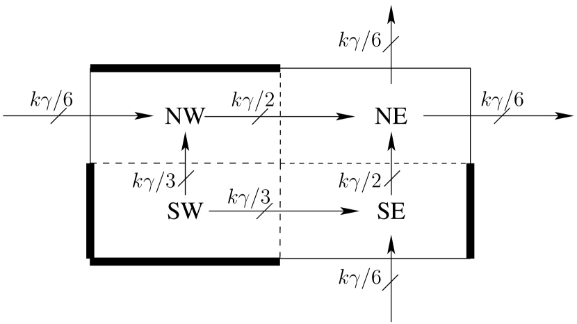
(a)

(b)

Figure 1: (a) Partitioning of a tile to quadrants. Thick lines represent “walls” that cannot be crosses by paths. Sources of requests may reside only in the SW quadrant of a tile. Maximum flow amounts crossing quadrant sides appear next to each side. Final destinations of paths are assumed (pessimistically) to be in the top row of the NE quadrant. (b) 4 types of requests within an $a\times b$ quadrant (in our case $a=b=k$). If the total flow destined to the north or east sides is at most their capacities then the detailed routing within the quadrant succeeds.

Crossbar routing. [EMP15].

Routing in each quadrant is simply an instance of routing in a (uni-directional) 2D grid where requests enter from two adjacent sides and exit from the opposite sides, that is, there are 4 types of requests: for $X\in\{S,W\}$ and $Y\in\{N,E\}$, let $\rm{req}(X\rightarrow Y)$ denote the set of path requests whose entry point to the tile is in the $X$ side and whose exit point is the $Y$ side. In fact, only the NE quadrant has all four types of requests cross it. The SE and NW quadrants have only two out of the four types. Figure 1(b) depicts such an instance of routing in one of the quadrants, in which requests arrive from the left and bottom sides and exit from the top and right sides. To show that crossbar routing within a quadrant succeeds in our case, we use the following claim from [EMP15].

Claim 2.

[EMP15, Proposition 5, Remark 6] Consider a $2$-dimensional directed $a\times b$ grid with edges of uniform capacity. A set of requests can be routed from the bottom and left boundaries of the grid to the opposite boundaries, if and only if the number of requests that should exit each side is at most the total capacity of edges crossing that side.

We conclude with the following claim.

Claim 3.

Detailed routing succeeds in routing all the requests in $R_{\textit{quad}}$ to create final paths for all requests in $R_{\textit{quad}}$.

Proof.

The sketch graph is a directed acyclic graph. Sort the tiles in topological order and within each tile, order the quadrants also in topological order: SW, NW, SE, NE, to get a topological order of all quadrants in the sketch graph. We prove by induction on the position of the quadrant in that topological order that detailed routing up to and including that quadrant succeeds. The claim for all SW quadrants follows because no path enters these quadrants from the outside and routing within these quadrants for requests with sources in these quadrants is identical to the paths computed by the randomized routing procedure. The SW quadrant of the first tile (according to the topological order) establishes also the basis of the induction. We now note that filtering ensures that the number of paths that cross each tile boundary is at most $2\lambda k\gamma<k\gamma/6$, and that the number of paths that cross each of the boundaries of each SW quadrant is at most $\gamma\cdot(k/3)$ (see Corollary 2). Further note that for each request entering a tile on a certain boundary and having to exit that tile on a certain other boundary, the sequence of quadrants that it has to cross within the tile is fixed. Therefore, the number of requests that enter each quadrant on a certain quadrant-boundary and the number of requests that have to exit this quadrant through a certain other quadrant-boundary is as depicted in Figure 1(b). The induction step follows by applying Claim 2. ∎

5.5 Approximation Ratio

Theorem 4.

The approximation ratio of the algorithm for packet requests in $R_{d_{\min},d_{\max}}$, for $d_{\min}=3\cdot\ln d_{\max}$, on network of arbitrary capacity $\gamma$, is constant in expectation.

Proof.

We follow the algorithm, as defined in Section 5.1, stage by stage.

Stage 1 computes a fractional maximum multi-commodity flow on a network with edge capacities $\lambda\cdot\gamma$ and with the requirement that all flows have bounded diameter of $2d_{\max}$. By Lemma 1, bounding path lengths in the MCF results in a solution of at least a $1/3$ fraction of the unrestricted one, and the scaling of the capacities in the space-time grid from $\gamma$ to $\lambda\cdot\gamma$ results in a solution which is at least a $\lambda=\Omega(1)$ fraction of the latter.

Stage 2 classifies the requests into $4$ classes and picks only the one for which the multi-commodity flow solution is the highest, hence resulting in a solution of at least a $1/4$ fraction of the solution of the previous stage.

Stage 3 applies a randomized rounding procedure to the flows that are picked in stage 2. The expected size of the solution is equal to the total flow left from the previous stage, but the solution might not be feasible.

Stage 4 applies a filtering procedure to the solution of the previous stage, in order to get a feasible solution on the sketch graph. By Claim 1, the expected size of this solution is at least a $1-O(1/k)$ fraction of the solution given by stage 3. Observe that $1-O(1/k)=\Omega(1)$ as $k=\Omega(\log\log\log n)$ in any relevant invocation of the algorithm. We note that the proof of Claim 1 uses the upper bound $d_{\max}$ on the distance that each packet has to travel.

Stage 5 further reduces the size of the solution when the algorithm selects a subset of the requests that have survived so far, using a maximum flow algorithm applied to each SW quadrant. This is done in order to allow for the solution to be feasible in the original space-time grid ($G^{st}$). By Corollary 2, the expected size of the solution after this stage is an $\Omega(1)$ fraction of the expected size before this stage. We note that the proof leading to Corollary 2 uses the lower bound $d_{\min}$ on the distance that each packet has to travel.

Stage 6 gives the final routing without further reducing the size of the solution.

We conclude that the algorithm (that we use for short, medium and long requests) is a randomized $O(1)$-approximation algorithm (in fact with respect to the fractional optimum). ∎

As explained at the top of Section 5, given the original problem with capacities $B$ and $c$, we run the randomized algorithm on a modified network with both edge and buffer capacities equal to $\gamma=\min\{B,c\}$. Since the optimal fractional solution on this modified network is only a $\max\{\gamma/B,\gamma/c\}$-fraction away from the optimal solution on the original network, we have the following.

Theorem 5.

The excepted approximation ratio of the algorithm for short, medium and long packets is $O(1)$ when $B=\Theta(c)$.

The above theorem, together with Lemma 2, concludes the proof of our main result as stated in Theorem 1.

Appendix A Reduction of Packet-Routing to Path Packing

A.1 Space-Time Transformation

A space-time transformation is a method to map schedules in a directed graph over time into paths in a directed acyclic graph [AAF96, ARSU02, AZ05, RR11]. Let $G=(V,E)$ denote a directed graph. The space-time transformation of $G$ is the acyclic directed infinite graph $G^{st}=(V^{st},E^{st})$, where: (i) $V^{st}\triangleq V\times\mathbb{N}$. We refer to every vertex $(v,t)$ as a copy of $v$. Namely, each vertex has a copy for every time step. We often refer to the copies of $v$ as the row of $v$. (ii) $E^{st}\triangleq E_{0}\cup E_{1}$where the set of forward edges is defined by $E_{0}\triangleq\{(u,t)\rightarrow(v,t+1)\>:\>(u,v)\in E~{},~{}t\in\mathbb{N}\}$ and the set of store edges is defined by $E_{1}\triangleq\{(u,t)\rightarrow(u,t+1)\>:\>u\in V,t\in\mathbb{N}\}$. (iii) The capacity of every forward edge is $c$, and the capacity of every store edge is $B$. Figure 2(a) depicts the space-time graph $G^{st}$ for a directed path over $n$ vertices. Note that we refer to a space-time vertex as $(v,t)$ even though the $x$-axis corresponds to time and the $y$-axis corresponds to the nodes. We often refer to $G^{st}$ as the space-time grid.

A.2 Untilting

The forward edges of the space-time graph $G^{st}$ are depicted in Fig. 2(a) by diagonal segments. We prefer the drawing of $G^{st}$ in which the edges are depicted by axis-parallel segments [RR11]. Indeed, the drawing is rectified by mapping the space-time vertex $(v,t)$ to the point $(v,t-v)$ so that store edges are horizontal and forward edges are vertical. Untilting simplifies the definition of tiles and the description of the routing. Figure 2(b) depicts the untilted space-time graph $G^{st}$ (e.g., the node $(2,1)$ is mapped to $(2,-1)$.).

(a)

(b)

Figure 2: The space-time graph $G^{st}$ before and after untilting [EM17].

A.3 The Reduction

A schedule $s_{i}$ for a packet request $r_{i}$ specifies a path $p_{i}$ in $G^{st}$ as follows. The path starts at $(a_{i},t_{i})$ and ends in a copy of $b_{i}$. The edges of $p_{i}$ are determined by the actions in $s_{i}$; a store action is mapped to a store edge, and a forward action is mapped to a forward edge. We conclude that a schedule $S$ induces a packing of paths such that at most $B$ paths cross every store edge, and at most $c$ paths cross every forward edge. Note that the length of the path $p_{i}$ equals the length of the schedule $s_{i}$. Hence we can reduce each packet request $r_{i}$ to a path request $r^{st}_{i}$ over the space-time graph. Vice versa, a packing of paths $\{p_{i}\}_{i\in I}$, where $p_{i}$ begins in $(a_{i},t_{i})$ and ends in a copy of $b_{i}$ induces a schedule. We conclude that there is a one-to-one correspondence between schedules and path packings.

Appendix B Multi-Commodity Flow Terminology

Network.

A network $N$ is a directed graph $G=(V,E)$, where edges have non-negative capacities $c(e)$. For a vertex $u\in V$, let $\mathsf{out}(u)$ denote the outward neighbors, namely the set $\{y\in V\mid(u,y)\in E\}$. Similarly, $\mathsf{in}(u)\triangleq\{x\in V\mid(x,u)\in E\}$.

Grid Network.

A grid network $N$ is a directed graph $G=(V,E)$ where $V=[n]\times\mathbb{N}$ and $(i,t_{1})\rightarrow(j,t_{2})$ is an edge in $E$ if and only if $t_{2}=t_{1}+1$ and $0\leq j-i\leq 1$.

Commodities/Requests.

A request $r_{i}$ is a pair $(a_{i},b_{i})$, where $a_{i}\in V$ is the source and $b_{i}\in V$ is the destination. We often refer to a request $r_{i}$ as commodity $i$. The request $r_{i}$ is to ship commodity $i$ from $a_{i}$ to $b_{i}$. All commodities have unit demand.

In the case of space-time grids, a request is a triple $(a_{i},b_{i},t_{i})$ where $a_{i},b_{i}\in[n]$ are the source and destination, and $t_{i}$ is the time of arrival. The source in the grid is the node $(a_{i},t_{i})$. The destination in the grid is any copy of $b_{i}$, namely, any vertex $(b_{i},t)$, where $t\in\mathbb{N}$ (see Section A.1).

Single commodity flow.

Consider commodity $i$. A single-commodity flow from $a_{i}$ to $b_{i}$ is a function $f_{i}:E\rightarrow\mathbb{R}^{\geq 0}$ that satisfies the following conditions:

1. Capacity constraints: for every edge $(u,v)\in E$, $0\leq f_{i}(u,v)\leq c(u,v)$.

2. Flow conservation: for every vertex $u\in V\setminus\{a_{i},b_{i}\}$

   $$\sum_{x\in\mathsf{in}(u)}f_{i}(x,u) =\sum_{y\in\mathsf{out}(u)}f_{i}(u,y).$$

3. Demand constraint: $|f_{i}|\leq 1$ (amount of flow $|f_{i}|$ defined below).

The amount of flow delivered by the flow $f$ is defined by

$$|f_{i}| \triangleq\sum_{y\in\mathsf{out}(a_{i})}f_{i}(a_{i},y)-\sum_{x\in\mathsf{in}(a_{i})}f_{i}(x,a_{i}).$$

The support of a flow $f_{i}$ is the set of edges $(u,v)$ such that $f_{i}(u,v)>0$. As cycles in the support of $f_{i}$ can be removed without decreasing $|f_{i}|$, one may assume that the support of $f_{i}$ is acyclic.

Multi-commodity flow (MCF).

In a multi-commodity flow (MCF) there is a set of commodities $I$, and, for each commodity $i\in I$, we have a source-destination pair denoted by $(a_{i},b_{i})$. Consider a sequence $F\triangleq\{f_{i}\}_{i\in I}$ of single-commodity flows, where each $f_{i}$ is a single commodity flow from the source vertex $a_{i}$ to the destination vertex $b_{i}$. We abuse notation, and let $F$ denote also the sum of the flows, namely $F:E\rightarrow\mathbb{R}$, where $F(e)\triangleq\sum_{i\in I}f_{i}(e)$, for every edge $e$. A sequence $F$ is a multi-commodity flow if, in addition to the requirements defined above for each flow $f_{i}$, $F$ satisfies the cumulative capacity constraints defined by:

for every edge $$(u,v)\in E ~{}~{}~{}F(u,v)\leq c(u,v).$$:

The throughput of an MCF $F\triangleq\{f_{i}\}_{i\in I}$ is defined to be $\sum_{i\in I}|f_{i}|$. In the maximum throughput MCF problem, the goal is to find an MCF $F$ that maximized the throughput.

An MCF is called all-or-nothing, if $|f_{i}|\in\{0,1\}$ for every commodity $i\in I$. An MCF is called unsplittable if the support of each flow is a simple path . An MCF is integral if it is both all-or-nothing and unsplittable. An MCF that is not integral is called a fractional MCF.

Appendix C Randomized Rounding Procedure

In this section we present material from [RT87] about randomized rounding. The proof of the Chernoff bound is also based on [You95].

Given an instance $F=\{f_{i}\}_{i\in I}$ of a fractional multi-commodity flow, we are interested in finding an integral (i.e., all-or-nothing and unsplittable) multi-commodity flow $F^{\prime}=\{f^{\prime}_{i}\}_{i\in I}$ such that the throughput of $F^{\prime}$ is as close to the throughput of $F$ as possible.

Observation 6.

As flows along cycles are easy to eliminate, we assume that the support of every flow $f_{i}\in F$ is acyclic.

We employ a randomized procedure, called randomized rounding, to obtain $F^{\prime}$ from $F$. We emphasize that all the random variables used in the procedure are independent. The procedure is divided into two parts. First, we flip random coins to decide which commodities are supplied. Next, we perform a random walk along the support of the supplied commodities. Each such walk is a simple path along which the supplied commodity is delivered. We describe the two parts in details below.

Deciding which commodities are supplied.

For each commodity, we first decide if $|f^{\prime}_{i}|=1$ or $|f^{\prime}_{i}|=0$. This decision is made by tossing a biased coin $b_{i}\in\{0,1\}$ such that

$$\mathbf{Pr}\left[\mathopen{b_{i}=1}\right] \triangleq|f_{i}|\leq 1.$$

If $b_{i}=1$, then we decide that $|f^{\prime}_{i}|=1$ Otherwise, if $b_{i}=0$, then we decide that $|f^{\prime}_{i}|=0$.

Assigning paths to the supplied commodities.

For each commodity $i$ that we decided to fully supply (i.e., $b_{i}=1$), we assign a simple path $P_{i}$ from its source $s_{i}$ to its destination $t_{i}$ by following a random walk along the support of $f_{i}$. At each node, the random walk proceeds by rolling a dice. The probabilities of the sides of the dice are proportional to the flow amounts. A detailed description of the computation of the path $P_{i}$ is given in Algorithm 1.

Algorithm 1 Algorithm for assigning a path $P_{i}$ to flow $f_{i}$.

1:$P_{i}\leftarrow\emptyset$.

2:$u\leftarrow s_{i}$

3:while $u\neq t_{i}$ do $\triangleright$ did not reach $t_{i}$ yet

4:     $v\leftarrow\textit{choose-next-vertex}(u)$.

5:     Add $(u,v)$ to $P_{i}$

6:     $u\leftarrow v$

7:end while

8:return $(P_{i})$.

9:procedure choose-next-vertex($u,f_{i}$)

10:     Let $\mathsf{out}(u,f_{i})$ denote the set of edges in the support of $f_{i}$ that emanate from $u$.

11:     Consider a dice $C(u,f_{i})$ with $|\mathsf{out}(u,f_{i})|$ sides. The side corresponding to an edge $(u,v)\in\mathsf{out}(u,f_{i})$ has probability $f_{i}{(u,v)}/(\sum_{(u,v^{\prime})\in\mathsf{out}(u,f_{i})}f_{i}(u,v^{\prime}))$.

12:     Let $v$ denote the outcome of a random roll of the dice $C(u,f_{i})$.

13:     return $(v)$

14:end procedure

Definition of $F^{\prime}$.

Each flow $f^{\prime}_{i}\in F^{\prime}$ is defined as follows. If $b_{i}=0$, then $f^{\prime}_{i}$ is identically zero. If $b_{i}=1$, then $f^{\prime}_{i}$ is defined by

$$f^{\prime}_{i}(u,v) \triangleq\begin{cases}1&\text{if $(u,v)\in P_{i}$,}\\ 0&\text{otherwise.}\end{cases}$$

Hence, $F^{\prime}=\{f^{\prime}_{i}\mid b_{i}=1\}$ is an all-or-nothing unsplittable flow, as required.

C.1 Expected flow per edge

The following claim can be proved by induction on the position of an edge in a topological ordering of the support of $f_{i}$.

Claim 4.

For every commodity $i$ and every edge $(u,v)\in E$:

$$\mathbf{Pr}\left[\mathopen{(u,v)\in P_{i}}\right] =f_{i}(u,v),$$

$$\mathbf{E}\left[{f^{\prime}_{i}(u,v)}\right] =f_{i}(u,v).$$

References

- [AAF96] Baruch Awerbuch, Yossi Azar, and Amos Fiat. Packet routing via min-cost circuit routing. In ISTCS, pages 37–42, 1996.
- [AKK09] Stanislav Angelov, Sanjeev Khanna, and Keshav Kunal. The network as a storage device: Dynamic routing with bounded buffers. Algorithmica, 55(1):71–94, 2009. (Appeared in APPROX-05).
- [AKOR03] William Aiello, Eyal Kushilevitz, Rafail Ostrovsky, and Adi Rosén. Dynamic routing on networks with fixed-size buffers. In SODA, pages 771–780, 2003.
- [ARSU02] Micah Adler, Arnold L. Rosenberg, Ramesh K. Sitaraman, and Walter Unger. Scheduling time-constrained communication in linear networks. Theory Comput. Syst., 35(6):599–623, 2002.
- [AZ05] Yossi Azar and Rafi Zachut. Packet routing and information gathering in lines, rings and trees. In ESA, pages 484–495, 2005. (See also manuscript in http://www.cs.tau.ac.il/~azar/).
- [EM10] Guy Even and Moti Medina. An O(logn)-Competitive Online Centralized Randomized Packet-Routing Algorithm for Lines. In ICALP (2), pages 139–150, 2010.
- [EM11] Guy Even and Moti Medina. Online packet-routing in grids with bounded buffers. In Proc. 23rd Ann. ACM Symp. on Parallelism in Algorithms and Architectures (SPAA), pages 215–224, 2011.
- [EM17] Guy Even and Moti Medina. Online packet-routing in grids with bounded buffers. Algorithmica, 78(3):819–868, 2017.
- [EMP15] Guy Even, Moti Medina, and Boaz Patt-Shamir. Better deterministic online packet routing on grids. In Proceedings of the 27th ACM on Symposium on Parallelism in Algorithms and Architectures, SPAA 2015, Portland, OR, USA, June 13-15, 2015, pages 284–293, 2015.
- [EMR16] Guy Even, Moti Medina, and Adi Rosén. A constant approximation algorithm for scheduling packets on line networks. In 24th Annual European Symposium on Algorithms, ESA 2016, August 22-24, 2016, Aarhus, Denmark, pages 40:1–40:16, 2016.
- [Kle96] Jon M Kleinberg. Approximation algorithms for disjoint paths problems. PhD thesis, Massachusetts Institute of Technology, 1996.
- [KT95] Jon M. Kleinberg and Éva Tardos. Disjoint paths in densely embedded graphs. In FOCS, pages 52–61, 1995. (See also manuscript in http://www.cs.cornell.edu/home/kleinber/).
- [Rag86] Prabhakar Raghavan. Randomized rounding and discrete ham-sandwich theorems: provably good algorithms for routing and packing problems. In Report UCB/CSD 87/312. Computer Science Division, University of California Berkeley, 1986.
- [RR11] Harald Räcke and Adi Rosén. Approximation algorithms for time-constrained scheduling on line networks. Theory Comput. Syst., 49(4):834–856, 2011.
- [RS11] Adi Rosén and Gabriel Scalosub. Rate vs. buffer size-greedy information gathering on the line. ACM Transactions on Algorithms, 7(3):32, 2011.
- [RT87] Prabhakar Raghavan and Clark D Tompson. Randomized rounding: a technique for provably good algorithms and algorithmic proofs. Combinatorica, 7(4):365–374, 1987.
- [You95] Neal E Young. Randomized rounding without solving the linear program. In SODA, volume 95, pages 170–178, 1995.