Dispersive shock waves and modulation theory

Abstract

There is growing physical and mathematical interest in the hydrodynamics of dissipationless/dispersive media. Since G. B. Whitham’s seminal publication fifty years ago that ushered in the mathematical study of dispersive hydrodynamics, there has been a significant body of work in this area. However, there has been no comprehensive survey of the field of dispersive hydrodynamics. Utilizing Whitham’s averaging theory as the primary mathematical tool, we review the rich mathematical developments over the past fifty years with an emphasis on physical applications. The fundamental, large scale, coherent excitation in dispersive hydrodynamic systems is an expanding, oscillatory dispersive shock wave or DSW. Both the macroscopic and microscopic properties of DSWs are analyzed in detail within the context of the universal, integrable, and foundational models for uni-directional (Korteweg-de Vries equation) and bi-directional (Nonlinear Schrödinger equation) dispersive hydrodynamics. A DSW fitting procedure that does not rely upon integrable structure yet reveals important macroscopic DSW properties is described. DSW theory is then applied to a number of physical applications: superfluids, nonlinear optics, geophysics, and fluid dynamics. Finally, we survey some of the more recent developments including non-classical DSWs, DSW interactions, DSWs in perturbed and inhomogeneous environments, and two-dimensional, oblique DSWs.

1 Introduction

Dispersive hydrodynamics is the domain concerned with fluid or fluid-like motion in which dissipation, e.g., viscosity, is negligible relative to wave dispersion. In conservative media such as superfluids, optical materials, and water waves, nonlinearity has the tendency to engender wavebreaking that is mediated by dispersion. Generically, the result of these processes is a multiscale, unsteady, coherent wave structure called a dispersive shock wave or DSW. This review is concerned with the mathematical study of dispersive shock waves and applications, principally via nonlinear wave modulation theory, often referred to as Whitham averaging [1].

1.1 Dispersive hydrodynamics

In classical fluid dynamics, unphysical hydrodynamic singularities (gradient catastrophe) are resolved by a transfer of energy from large to small spatial scales accompanied by an increase in entropy. This results in a smooth but rapid transition in hydrodynamic and thermodynamic quantities, a shock wave that moves faster than the local speed of sound. These irreversible processes are fundamental to classical, dissipative hydrodynamics. In contrast, when singularities are resolved by a conservative, reversible process such as wave dispersion, the resulting dynamics are quite different. Rather than the generation of a turbulent energy cascade, gradient catastrophe in dispersive hydrodynamic media leads to the generation of an expanding nonlinear wavetrain, a dispersive shock wave. Dispersive hydrodynamics is therefore quite different from its dissipative hydrodynamic analogue. Nevertheless, the rich theory of classical hydrodynamics provides a natural compass that is helpful in navigating the relatively new field of dispersive hydrodynamics, e.g., Riemann problems, characteristics, shock loci, admissibility, et cetera.

DSWs have recently garnered attention in connection with ground breaking experiments on ultracold atoms [2, 3, 4, 5, 6, 7] (Figs. 1a,b) and in optical media [8, 9, 10, 11, 12, 13, 14, 15, 16] (Figs. 1c,d), where they have been referred to as quantum or optical shocks, respectively. Figures 1e,f show a Helium II surface wave pattern above 1e and below 1f the superfluid temperature [17]. The development of rank ordered, stationary concentric rings in this hydraulic jump are indicative of DSWs. Dispersive shock waves have also been observed in intense electron beams [18] and rarefied plasma [19, 20] over sufficiently short time scales.

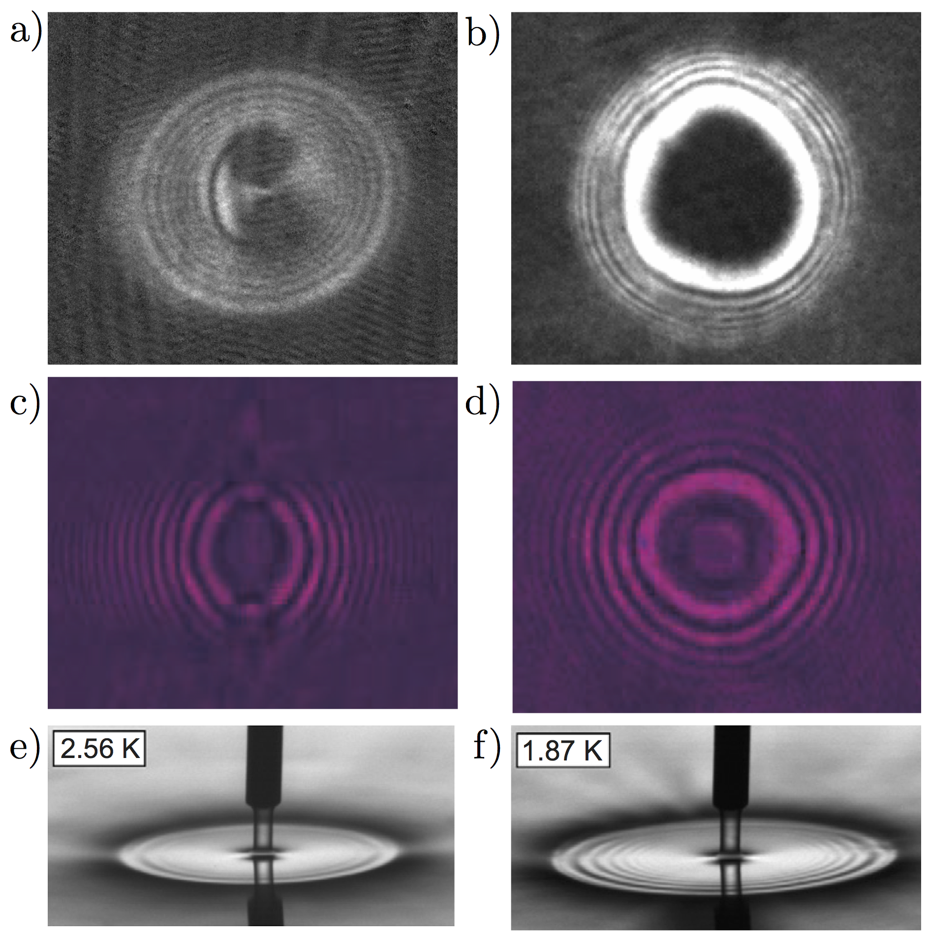
Figure 1: Dispersive shock waves. a,b) Blast waves in a Bose-Einstein condensate with expansion post (a) and during (b) laser pulse application [4]. c,d) Nonlinear diffraction of an elliptical (c) and circular (d) Gaussian beam after propagation through a photorefractive crystal. Reprinted by permission from Macmillan Publishers Ltd: Nature Physics [10], copyright 2007. e,f) Hydraulic jump in liquid He II above (e) and below (f) the superfluid transition temperature 2.17 K. Reprinted from [17] with permission from Elsevier.

Dispersive hydrodynamics are not limited to exotic media but can also occur in geophysics: stratified environments of the ocean and atmosphere where the dispersive hydrodynamic medium is the interface between two fluids, e.g., the ocean surface and air [21, 22, 23, 24, 25, 26, 27], an internal ocean pycnocline [28, 29, 30], or lower and upper atmospheric layers [31, 32, 33]. Here, the dispersive hydrodynamic medium is the interface itself. The conservation of mass enables approximately frictionless interfacial dynamics. DSWs in these systems are often referred to as undular bores or roll clouds. Striking examples of DSWs include Morning Glory roll clouds and mountain waves (Fig. 2). Shallow water undular bores or oscillatory hydraulic jumps are one of the earliest observed DSWs (see Secs. 4.2.2 and 9). Internal ocean wave DSWs are quite prevalent, especially in coastal regions during the summer months [28] (see Sec. 7). An additional system fitting into this category is the interfacial dynamics of two Stokes fluids with high viscosity contrast, proposed as a model of mantle magma dynamics [34, 35] (see Sec. 4.2.1). Indeed, any approximately conservative medium exhibiting wave dispersion can be classified dispersive hydrodynamic over sufficiently short spatio-temporal scales. All of these DSW examples exhibit a common, rank ordered structure of oscillations.

DSWs are believed to play an important role in a number of atmospheric and oceanic events such as thunderstorm initiation [32], coastal tsunami propagation [24], [36] and internal ocean transport [29]. Under appropriate conditions, all the aforementioned media exhibit the requisite dispersive hydrodynamic features of nonlinearity and dispersion. These features can be modeled, in the simplest case, by a hyperbolic system with dispersive corrections

$$\mathbf{u}_{t}+\nabla\cdot\mathbf{F}(\mathbf{u})=\nabla\cdot\mathbf{D}[\mathbf{u}],$$ (1.1)

where $\mathbf{u}=\mathbf{u}(\mathbf{x},t)$ is the state vector, $\mathbf{F}$ is the nonlinear flux tensor, and $\mathbf{D}$ is an integro-differential dispersive operator (in general, a 2-tensor), distinguished by giving rise to a real-valued dispersion relation, $\omega(\mathbf{k},\mathbf{u}_{0})$–found by linearizing equation (1.1) according to $\mathbf{u}(\mathbf{x},t)=\mathbf{u}_{0}+\mathbf{v}e^{i(\mathbf{k}\cdot\mathbf{x}-\omega t)}$, $|\mathbf{v}|\to 0$–such that the dispersion sign defined as $\mathrm{sgn}[\det(\partial_{k_{i}k_{j}}\omega)]$ is not identically zero. Partial differential equations (PDE) of the type in eq. (1.1) will be the focus of this review. Suppose the evolution described by (1.1) is characterized by two distinct spatio-temporal scales: the hydrodynamic scale $\Delta x\sim l$, $\Delta t\sim l/c_{s}$ ($c_{s}$ is the characteristic dispersionless, hyperbolic speed in the system, i.e., the speed of sound), typically specified by initial or boundary conditions, and the dispersive scale $\Delta x\sim L$, $\Delta t\sim L/c_{p}$ ($c_{p}$ is the typical phase velocity), where $L$ is the typical wavelength of dispersive waves, the intrinsic coherence scale of the system. The motion in such a system can be classified as dispersive-hydrodynamic if $\varepsilon=L/l\ll 1$.

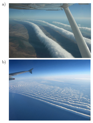
Figure 2: Atmospheric dispersive shock waves. a) Morning glory roll cloud (copyright Mick Petroff, Creative Commons 3.0, 2009). b) Mountain waves (photo courtesy of the COMET${}^{\textrm{\textregistered}}$ Program).

The scalar, one-dimensional, uni-directional version of eq. (1.1) takes the form

$$u_{t}+f(u)_{x}=D[u]_{x}.$$ (1.2)

When $D\equiv 0$ and $f^{\prime\prime}(u)\neq 0$, smooth initial data for (1.2) can develop singularities in finite time [1]. The inclusion of dispersion, $D\neq 0$, regularizes the dynamics. The equations of this type are abundant but perhaps the most ubiquitous is the Korteweg-de Vries (KdV) equation [37, 38] where $f(u)=\frac{1}{2}u^{2}$ and $D[u]=-u_{xx}$. The choice of convective nonlinearity $f(u)$ and the dispersive operator $D[u]$ has a significant impact on the resultant dispersive hydrodynamics. In this review, we will explore the dispersive hydrodynamics of several models in the form (1.2) with particular emphasis on KdV.

A pervasive example of a bi-directional system of two dispersive hydrodynamic equations are the dispersive Euler equations

$$\begin{split}\rho_{t}+(\rho u)_{x}&=D_{1}[\rho,u]_{x}\\ (\rho u)_{t}+\left(\rho u^{2}+P(\rho)\right)_{x}&=D_{2}[\rho,u]_{x},\end{split}$$ (1.3)

where $\rho\geq 0$ is interpreted as the dispersive fluid density, $u$ is the fluid’s velocity, and $P(\rho)$ is a given constitutive law for the pressure. In the absence of dispersion $D_{1}=D_{2}\equiv 0$, equations (1.3) are known as the Euler $P$-system. The $P$-system is hyperbolic so long as $P^{\prime}(\rho)>0$ and therefore admits the sound speed $c(\rho)=\sqrt{P^{\prime}(\rho)}$. A number of well-known model equations fit within this framework, including the generalized Nonlinear Schrödinger (gNLS) equation

$$i\psi_{t}+\frac{1}{2}\psi_{xx}-f(|\psi|^{2})\psi=0,$$ (1.4)

where $f$ is a smooth, positive, monotonically increasing function of its argument. In order to write equation (1.4) in the hydrodynamic form (1.3), we utilize the transformation to magnitude and phase variables

$$\psi=\sqrt{\rho}e^{i\phi},\quad u=\phi_{x},$$ (1.5)

known as the Madelung transformation. After insertion of (1.5) into (1.4) and equating real and imaginary parts, the gNLS equation takes the hydrodynamic form (1.3) with

$$\begin{split}P(\rho)&=\int_{0}^{\rho}sf^{\prime}(s)\,\mathrm{d}s,\\ D_{1}[\rho,u]&\equiv 0,\quad D_{2}[\rho,u]=\frac{1}{4}\rho(\ln\rho)_{xx}.\end{split}$$ (1.6)

When $f(\rho)=\rho$, we obtain the integrable Nonlinear Schrödinger (NLS) equation.

1.2 Anatomy of a dispersive shock wave

In very general terms, DSWs are multi-scale, unsteady, nonlinear coherent wave structures that are characterized by two complementary identities. When viewed locally, i.e., over a small region of space and time, DSWs display periodic, or quasiperiodic structure (see Fig. 3 inset), forming due to the interplay between nonlinear and dispersive effects. Over a larger region covering multiple wave oscillations, the DSW wavetrain exhibits slow modulation of the wave’s parameters (amplitude, frequency, mean), and this modulation itself is a nonlinear hyperbolic wave (see Fig. 3). This kind of “dispersive-hyperbolic” duality of modulated waves is not uncommon in linear wave theory but DSWs prominently display it over the full range of nonlinearity, from a weakly nonlinear regime to solitary waves realized as an integral part of the modulated wavetrain. A DSW connects two, disparate, non-oscillatory states, which are either constant or slowly varying, an important distinction from a generic nonlinear wavetrain [39].

The striking manifestation of nonlinearity in a DSW is that it is characterized by at least two distinct speeds of propagation, those of its leading $s_{+}$ and trailing $s_{-}$ edges as shown in Fig. 3. These two DSW speeds bifurcate from the linear group velocity, a striking realization of the splitting of the doubly degenerate characteristic speed from linear wave theory [1].

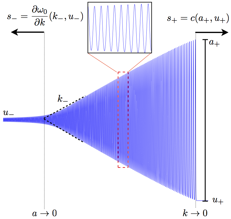
Figure 3: Schematic of a dispersive shock wave’s macroscopic and microscopic (inset) structure.

As depicted in the DSW schematic of Fig. 3, the two distinct speeds of propagation correspond to a small amplitude, harmonic limit $a\to 0$ of the modulated wavetrain and a large amplitude solitary wave limit where the wavenumber $k$ vanishes. As described in Sec. 4, these distinguished limits and an additional simple wave assumption enable the determination of DSW edge speeds: the linear group velocity determines the harmonic edge speed and the solitary wave amplitude-speed relation determines the opposite edge speed. Associated with the harmonic and solitary wave speeds are a characteristic wavenumber of the weakly nonlinear harmonic edge wavepacket, denoted $k_{-}$ in Fig. 3, and the solitary wave amplitude, denoted $a_{+}$ in Fig. 3. The DSW speeds, characteristic wavenumber, amplitude, and DSW envelope constitute the macroscopic observables of a DSW. The slowly modulated wave connecting the leading and trailing edges describes the microscopic DSW structure (see Fig. 3 inset).

Because DSWs exhibit two distinct edges, it is natural to define the DSW orientation $d$. When the solitary wave is at the DSW leading edge (rightmost), as in Fig. 3, $d=1$; $d=-1$ otherwise. Associated with the solitary wave edge is the polarity $p$, depending upon whether the edge is a wave of elevation ($p=1$, as in Fig. 3) or depression ($p=-1$). Figure 4 depicts a DSW classification according to orientation and polarity. For scalar dispersive hydrodynamic equations (1.1), the orientation and polarity of a DSW are related to the curvature of the dispersion and the nonlinear flux [40].

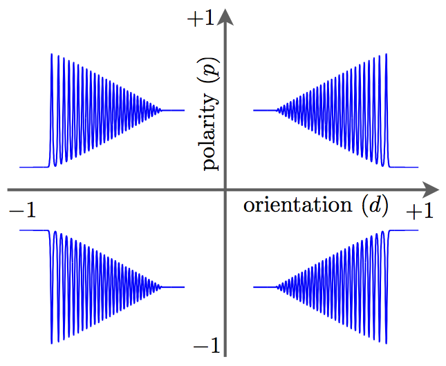
Figure 4: Orientation and polarity of a DSW.

1.3 Dispersive vs. dissipative-dispersive shocks

The generation of DSWs represents a universal mechanism to resolve unphysical hydrodynamic singularities in dispersive conservative media, so their fundamental role in such media is similar to that of viscous shock waves (VSWs) in classical gas and fluid dynamics. At the same time, DSWs are sharply distinct from their well-studied viscous counterpart both in terms of physical significance and mathematical description. First of all, DSWs, unlike VSWs, do not dissipate energy. The potential energy of the jump in hydrodynamic quantities across a DSW leads to kinetic energy associated with nonlinear wave generation and is not accompanied by an increase in entropy. An increase in entropy as a shock is traversed, on the other hand, is a defining property of VSWs [41]. Two salient features of DSWs, their oscillatory microscopic structure and unsteady macroscopic dynamics, make the distinction between DSWs and VSWs particularly evident. Indeed, the internal oscillatory structure of DSWs is in sharp contrast with the monotone structure of VSWs. But it is the second unique feature of DSWs, their unsteady, expanding nature, that makes DSWs so radically distinct from VSWs. VSWs are characterized by a fixed width and a single speed of propagation, the latter being determined by a balance of physical integrals of motion (e.g., mass and momentum) across the shock, not depending on the details of its internal structure. The unsteady dynamics of DSWs have far-reaching physical and mathematical implications, among which are the inapplicability of classical Rankine-Hugoniot relations and the inseparability of the description of macroscopic DSW dynamics from the analysis of its nonlinear oscillatory microstructure.

In order to illustrate the distinction between DSWs and VSWs, we consider a model equation incorporating nonlinearity, dispersion, and dissipation in the Korteweg-de Vries-Burger’s (KdVB) equation

$$u_{t}+uu_{x}+\mu u_{xxx}=\nu u_{xx},$$ (1.7)

where $\mu\in\mathbb{R}$ is the dispersion coefficient and $\nu\geq 0$ is the dissipation coefficient. Diffusive-dispersive dynamics essentially reducible to the KdVB equation (1.7) arise in the original theory of undular bores by Benjamin and Lighthill [42] (see also [1]) and in the theory of collisionless shocks in rarefied plasma due to Sagdeev [43, 44] (see also the notable publication [45] in a popular magazine) and others (see, e.g., [46]). The KdVB equation has also recently been invoked as a universal model of cold atom hydrodynamics [47]. When $\mu=\nu=0$ (Hopf equation), decreasing initial data leads to singularity formation in finite time [1]. When $\mu\neq 0$ and $\nu=0$ (KdV equation), the singularity is resolved by a DSW whose structure is described via a weak limit as $\mu\to 0^{+}$ or $\mu\to 0^{-}$ according to the Whitham modulation equations [48, 49, 50] (see Sec. 3.1). The direction $\mu$ approaches zero determines the DSW orientation $d=\mathrm{sgn}\,\mu$ and polarity $p=\mathrm{sgn}\,\mu$. The purely dissipative regularization $\mu=0$ and $\nu\to 0^{+}$ (Burger’s equation) strongly converges to a discontinuous solution, a VSW, with shock speed determined by the Rankine-Hugoniot jump conditions [1].

The regularization where both dissipation and dispersion are included (KdVB equation) crucially depends on the ratio $\delta=\nu/\sqrt{|\mu|}$ [46, 51, 52, 53]. When $\delta\to 0$ and $\mu\to 0^{+}$ or $\mu\to 0^{-}$, i.e., a dispersion dominated regularization, the behavior is again described by a DSW. If $\delta>\delta_{0}>0$ and $\nu\to 0^{+}$, $\mu\to 0^{\pm}$, the regularization is dissipatively dominated and the solution strongly converges to the same VSW solution as in Burger’s equation. The transition between these two limiting cases, DSW and VSW, can be understood by taking $\delta>0$ fixed (dissipation balancing dispersion) and seeking traveling wave (TW) solutions in the form $u(x,t)\to u(\xi)$, $\xi=(x-st)/\sqrt{|\mu|}$ with $u(\pm\infty)=u_{\pm}$. Inserting the TW ansatz into eq. (1.7), integrating once and letting $v=u^{\prime}$, we obtain the first order system of ordinary differential equations (ODE)

$$u^{\prime}=v,\quad(\mathrm{sgn}\,\mu)v^{\prime}=\delta v-\frac{1}{2}(u^{2}+u_{-}u_{+})+su.$$ (1.8)

The TW speed $s=\frac{1}{2}(u_{+}+u_{-})$, determined by the boundary conditions, satisfies the Rankine-Hugoniot jump conditions. The phase portrait of the system, shown in Fig. 5a for $\mu=1$, has two equilibria $(u,v)=(u_{\pm},0)$, one of which is a saddle point, $(u_{\mathrm{sgn}\,\mu},0)$, and the other is a stable ($\mu<0$) or unstable ($\mu>0$) node or spiral, depending on whether the eigenvalues of the linearized system

$$\lambda_{\pm}(u)=\frac{1}{2}\left(\delta\,\mathrm{sgn}\,\mu\pm\sqrt{\delta^{2}+4(s-u)\mathrm{sgn}\,\mu}\right),$$

are real ($\delta\geq\sqrt{2\Delta}$) or complex ($\delta<\sqrt{2\Delta}$), respectively. The jump across the TW, $\Delta=u_{-}-u_{+}>0$, corresponds to the Lax entropy condition [41]. The structure of the TW changes from a monotonic to an oscillatory profile as $\delta$ is decreased across the critical value $\sqrt{2\Delta}$. Further analysis shows that for $0<\delta\ll 1$, the amplitude of the largest oscillation in the TW profile is approximately $a=\frac{3}{2}\Delta$ [51]. This corresponds to the outermost trajectory in the phase plane, intersecting $(u,v)=(1.5,0)$ in Fig. 5a.

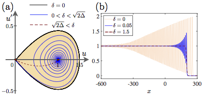
Figure 5: (a) Phase plane depicting KdVB TW solutions connecting $u_{+}=0<u_{-}=1$ with $\mu=1$ via a monotone TW (dashed, strong dissipation) or an oscillatory TW (solid spiral, weak dissipation). The KdV soliton (solid homoclinic orbit, zero dissipation) encloses the union of all KdV periodic orbits spanned across a DSW. (b) Numerical solutions of KdVB at $t=400$ with step-like initial data at the origin and the same $\delta$, $\mu$ as in (a). TWs ($\delta>0$) and DSWs ($\delta=0$) are attractors for the dynamics.

For $\delta=0$, however, the (un)stable equilibrium becomes a center, i.e., with imaginary eigenvalues, and a TW connecting $u_{+}$ and $u_{-}$ no longer exists. Instead, there is a homoclinic orbit connecting the saddle point to itself, and the corresponding TW is a KdV soliton. Enclosed within this homoclinic orbit are periodic orbits representing KdV periodic TW solutions. Numerical solutions to eq. (1.7) with step-like initial data for the same three values $\delta>\sqrt{2\Delta}$, $0<\delta<\sqrt{2\Delta}$, and $\delta=0$ used in Fig. 5a are shown in Fig. 5b. We observe that the $\delta>0$ solutions rapidly approach KdVB TWs and that the TWs with $0<\delta<\sqrt{2\Delta}$ exhibit oscillatory structure whose signature is inherited by the orientation and polarity of the corresponding $\delta=0$ DSW. The analysis in Sec. 3.1 shows that a DSW is described by a modulation of the periodic TWs from the zero amplitude, equilibrium solution to the infinite period, soliton, homoclinic solution. This allows us to identify the key distinction between VSWs and DSWs:

• The VSW can be modeled by a TW solution to an ODE (a single heteroclinic orbit).

• The DSW can be modeled by a PDE modulation of the periodic TW (effectively, a continuous family of periodic orbits that is traversed across the wavetrain).

Note also that the DSW soliton edge amplitude is $a_{\mathrm{sgn}\,\mu}=2\Delta$, moving with speed $s_{\mathrm{sgn}\,\mu}=\frac{1}{3}(u_{-}+u_{+}+u_{(-\mathrm{sgn}\,\mu)})$ (see Sec. 3.1), different from the KdVB TW.

1.4 Aim of this Review

When writing a review article, there is always a competition between breadth and depth. We initially intended to survey a broad set of problems related to DSWs in dispersive hydrodynamics, while touching upon the theoretical tools involved. However, while there are texts [1, 54], a shorter review [55], and articles with lengthy introductory material [56, 57, 40] covering some aspects of DSW theory, we felt that a more comprehensive review of the fundamental mathematical tools would fill an important void. Dispersive hydrodynamics is experiencing significant development in recent years as evidenced by this dedicated special issue. The bulk of this review surveys the fundamentals of modulation theory (Sec. 2), the dispersive regularization of shock waves in integrable systems (KdV and NLS, Sec. 3), and the construction of DSWs in non-integrable systems (Sec. 4). The latter sections provide an overview of some more recent developments including non-classical DSWs (Sec. 5), DSW interactions (Sec. 6), DSWs in inhomogeneous environments (Secs. 7, 8), and multidimensional, steady, oblique DSWs (Sec. 9).

2 Mathematical tools of DSW modulation theory

The mathematical description of DSWs involves a synthesis of methods from hyperbolic quasi-linear systems, asymptotics, and soliton theory. One of the primary tools is nonlinear wave modulation theory, introduced by Whitham in 1965 [48]. Whitham theory and an additional technique, matched asymptotic analysis, are approximate methods that have demonstrated practical impact in a wide variety of problems despite their formal nature. Rigorous, exact solution methods such as the Inverse Scattering Transform (IST) and the associated Riemann-Hilbert steepest descent method are quite powerful, but only apply to a limited class of integrable systems and problems. The PDE of dispersive hydrodynamics encompass a range of integrable systems such as the KdV, NLS, and Kadomtsev-Petviashvili (KP) equations as well as their nonintegrable generalizations. In this section, we review properties of quasi-linear systems and Whitham theory.

2.1 Hydrodynamic type systems

2.1.1 Basic notions

In this subsection, we present a brief account of some basic notions and techniques from the theory of one-dimensional quasi-linear systems. A detailed description can be found in [58, 59].

Systems of first-order, homogeneous, quasi-linear partial differential equations (PDEs)

$${\bf u}_{t}+\mathrm{A}({\bf u}){\bf u}_{x}=0\,,$$ (2.1)

where ${\bf u}(x,t)=\{u_{1},u_{2},\dots,u_{N}\}\in\mathbb{R}^{N}$ and $\mathrm{A}(\mathbf{u})$ is an $N\times N$ matrix, are often called hydrodynamic type systems [60]. Such systems arise in the modeling of wave processes in continuum mechanics, plasma physics, magnetohydrodynamics etc. In the context of DSW theory, hydrodynamic type systems appear in two ways: (i) as the dispersionless ($\mathbf{D}\equiv 0$) limit of a dispersive hydrodynamic system (1.1); (ii) as Whitham modulation systems obtained by averaging the dispersive hydrodynamic system (1.1) over a family of periodic or quasi-periodic solutions.

If the equation

$$\frac{\partial}{\partial t}P({\bf u})+\frac{\partial}{\partial x}Q({\bf u})=0,$$ (2.2)

where $P({\bf u})$ and $Q({\bf u})$ are some scalar functions, is a consequence of the hydrodynamic type system (2.1) for any solution, then it is called a hydrodynamic conservation law of system (2.1). We note that in models arising in continuum physics, hydrodynamic type systems (2.1) are often deduced from a system of conservation laws expressing fundamental physical principles such as conservation of mass, momentum, energy, etc. In this case, one assumes that the relevant Jacobians are finite and non-singular. The number of independent conservation laws for the system (2.1) could be less, equal or greater than $N$. Sometimes hydrodynamic type systems have an infinite number of conservation laws. This property is usually linked to integrability in the sense of the generalized hodograph transform (see Sec. 2.1.3 below).

The curve $x(t)$ is called a characteristic of the system (2.1) if

$$\frac{dx}{dt}=\lambda,\qquad\det|\mathrm{A}-\lambda I|=0,$$ (2.3)

where ${I}$ is the $N\times N$ identity matrix. The eigenvalues $\lambda=V_{j}$, $j=1,\dots,N$ of the matrix $\mathrm{A}$, are called the characteristic velocities. Importantly, since $\mathrm{A}=\mathrm{A}({\bf u})$, the characteristics of the hydrodynamic type system (2.1) generally depend on the solution ${\bf u}(x,t)$.

Let ${\bf l}^{(k)}({\bf u})$ be the left eigenvector of the matrix $\mathrm{A}$ corresponding to the eigenvalue $V_{k}$. The system (2.1) is called hyperbolic if all the eigenvalues $V_{k}$ are real,

$$V_{1}({\bf u})\leqslant V_{2}({\bf u})\leqslant\dots\leqslant V_{N}({\bf u})\,,$$ (2.4)

and the eigenvectors ${\bf l}^{(k)}$ form a basis in $\mathbb{R}^{N}$. The system is called strictly hyperbolic if all eigenvalues $V_{k}$ are real and distinct

$$V_{1}({\bf u})<V_{2}({\bf u})<\dots<V_{N}({\bf u})\,.$$ (2.5)

A consequence of the system (2.1)

$${\bf l}^{(k)}\cdot({\bf u}_{t}+\mathrm{A}{\bf u}_{x})={\bf l}^{(k)}\cdot({\bf u}_{t}+V_{k}{\bf u}_{x})=0,$$ (2.6)

is called a characteristic relation of (2.1). For a strictly hyperbolic system (2.1), there are $N$ independent characteristic relations (2.6), which form a system equivalent to (2.1) called the characteristic form of (2.1). Each equation in the characteristic form contains differentiation only in a single direction of the $(x,t)$-plane, $\left(\frac{d{\bf u}}{dt}\right)_{k}=\left(\frac{\partial}{\partial t}+V_{k}\frac{\partial}{\partial x}\right){\bf u}$, so the system (2.1) transforms into a system of $N$ ODEs along $N$ characteristic directions.

Each characteristic relation (2.6) introduces the differential form

$${\bf l}^{(k)}\cdot d{\mathbf{u}}=l^{(k)}_{1}du_{1}+l^{(k)}_{2}du_{2}+\dots+l^{(k)}_{N}du_{N},$$ (2.7)

which vanishes on the $k$-th characteristic. If this form is integrable, then it is possible to introduce a new variable $r_{k}({\mathbf{u}})$ such that

$$dr_{k}=\mu{\bf l}^{(k)}\cdot d{\mathbf{u}},$$ (2.8)

for some $\mu({\bf u})$ called the integrating factor. Such a variable is called a Riemann invariant. If all $N$ characteristic forms (2.6) are integrable, then the system (2.1) assumes the diagonal or Riemann form

$$\frac{\partial r_{k}}{\partial t}+V_{k}({\bf r})\frac{\partial r_{k}}{\partial x}=0\,,\qquad k=1,\dots,N,$$ (2.9)

where we have used the shorthand notation $V_{k}({\bf r})\equiv V_{k}({\bf u}(\bf r))$ and assumed invertibility of the mapping ${\bf u}\mapsto{\bf r}$. One can see that each Riemann invariant $r_{k}$ is constant along the characteristic $dx/dt=V_{k}$.

Riemann invariants always exist if $N=2$ but generally do not exist if $N>2$. Each Riemann invariant $r_{k}$ is determined up to an arbitrary function of a single variable so that $F(r_{k})$ is also a Riemann invariant for any differentiable function $F$ of a single variable.

There is no general method for the computation of Riemann invariants (if they exist) for a given hydrodynamic type system (2.1). However, for the important class of hydrodynamic type systems obtained by Whitham averaging of dispersive-hydrodynamic systems (1.1) (see Sec. 2.2 below), the existence of Riemann invariants was shown to be intimately related to the integrability of the original equations via the IST. For such systems, there is an effective method of finding Riemann invariants using finite-gap integration theory (a periodic analogue of the IST method) [61, 54].

The property of strict hyperbolicity (2.5) for Whitham modulation systems can be maintained even when characteristic velocities merge. Strict hyperbolicity for such systems is retained due to the reduction of the system order $N$ so that the merged velocity defines a regular characteristic. For diagonal Whitham systems (2.9), this is taken into account by the following modification of the definition of strict hyperbolicity:

$$V_{j}=V_{k}\ \Longleftrightarrow\ r_{j}=r_{k}\quad\forall\,j,~{}k=1,\dots,N.$$ (2.10)

For non-strictly hyperbolic diagonal systems, there could be two or more distinct Riemann invariants associated with the same characteristic velocity $V_{k}$. In terms of the original system (2.1) (when it is diagonalizable) non-strict hyperbolicity is related to non-invertibility of the mapping ${\bf u}\mapsto{\bf r}$.

The $k$-th characteristic family of the diagonal system (2.9) is called genuinely nonlinear if

$$\partial_{k}V_{k}\neq 0,\quad\hbox{where}\quad\partial_{k}\equiv\frac{\partial}{\partial r_{k}}.$$ (2.11)

If (2.11) holds for all $k$, then the system (2.9) is called genuinely nonlinear. For a scalar conservation law $u_{t}+f(u)_{x}=0$, the condition of genuine nonlinearity is nonzero curvature of the flux, $f^{\prime\prime}(u)\neq 0$ for all $u$. The characteristic family $\frac{dx}{dt}=V_{k}$ is called linearly degenerate if $\partial_{k}V_{k}=0$. The system (2.9) is called linearly degenerate if $\partial_{k}V_{k}=0$ for all $k=1,\dots,N$.

The notions of genuine nonlinearity and linear degeneracy can be generalized to non-diagonal systems (2.1). The $k$-th characteristic family of the system (2.1) is genuinely nonlinear if [41]

$$\nabla_{\bf u}V_{k}\cdot{\bf p}^{(k)}\neq 0\,,$$ (2.12)

where ${\bf p}^{(k)}({\bf u})$ is the right eigenvector of the matrix $\mathrm{A}$ corresponding to the eigenvalue $V_{k}$.

If the system (2.1) is non-strictly hyperbolic, it is not genuinely nonlinear as well [59]. The converse is generally not true.

Finally, we introduce the definition of the integral curve of the vector field ${\bf p}^{(k)}$ as a solution of the system of $N$ ODE

$${\bf v}^{\prime}(s)={\bf p}^{(k)}({\bf v}(s)),$$ (2.13)

where $s$ is a parameter. One can see from (2.12), (2.13) that the $k$-th characteristic field is genuinely nonlinear if the characterisic velocity $V_{k}$ is monotone along the integral curve.

2.1.2 Simple waves

Closely related to the notion of a Riemann invariant is the notion of a simple wave or Riemann wave, playing an especially important role in the DSW theory. We first assume that the system (2.1) is strictly hyperbolic and genuinely nonlinear.

A simple wave is a particular solution of (2.1) such that all components of the vector ${\bf u}$ depend on the same quantity $\alpha(x,t)$,

$${u_{j}}=u_{j}(\alpha(x,t)),\qquad j=1,\dots,N.$$ (2.14)

Substituting (2.14) into (2.1), we obtain the system of ODE

$$(\mathrm{A}-\lambda I)\frac{d{\bf u}}{d\alpha}=0\,,\quad\lambda=-\frac{\alpha_{t}}{\alpha_{x}}\,.$$ (2.15)

A nontrivial solution of (2.15) for ${\bf u}(\alpha)$ is possible only if $\lambda=V_{k}$, for some $k\in\{1,\dots,N\}$. Then for each $k$, the solution of the algebraic system in (2.15) yields a system of $N$ integral curves ${\bf u}^{\prime}={\bf p}^{(k)}({\bf u}(\alpha))$ (cf. (2.13)). The second equation in (2.15) can be written as a scalar PDE

$$\alpha_{t}+V_{k}({\bf u}(\alpha))\alpha_{x}=0.$$ (2.16)

Because the system (2.1) was assumed strictly hyperbolic, it has $N$ families of simple wave solutions.

Since $\alpha=const$ along the characteristic $dx/dt=V_{k}({\bf u}(\alpha))$, this characteristic represents a straight line in the $x,t$ plane. All the other the characteristics are curvilinear. In particular, if $\alpha(x,t)=f(x/t)$, where $f^{\prime}\neq 0$, equation (2.16) implies $V_{k}=x/t$. Such similarity solutions play a particularly important role in DSW theory. Let $s=x/t$. Then for the similarity solution, $\frac{\,\mathrm{d}}{\,\mathrm{d}s}V_{k}=(\frac{\,\mathrm{d}}{\,\mathrm{d}\alpha}V_{k})f^{\prime}(s)=1$ and so $\frac{\,\mathrm{d}}{\,\mathrm{d}\alpha}V_{k}=\nabla_{\bf u}V_{k}\cdot\frac{\,\mathrm{d}}{\,\mathrm{d}\alpha}{\bf u}=\nabla_{\bf u}V_{k}\cdot\mathbf{p}^{(k)}\neq 0$ (cf. (2.12)). Thus, the similarity solution of (2.1) exists only if (2.1) is genuinely nonlinear for all ${\bf u}$ involved.

The $k$-wave curve associated with (2.1) is the curve $\mathbf{u}(\alpha)$ in $\mathbb{R}^{N}$ parametrized by $\alpha$ associated with the $k^{\mathrm{th}}$ characteristic family where $V_{k}(\mathbf{u}(\alpha))=x/t$. The curve identifies the states that can be continuously connected by a simple wave in the $k^{\mathrm{th}}$ characteristic family. Suppose two states $\mathbf{u}_{\pm}$ lie on the $k$-wave curve according to $\mathbf{u}_{\pm}=\mathbf{u}(\alpha_{\pm})$ where $\alpha_{-}<\alpha_{+}$. Then a global, continuous solution to (2.16) exists so long as $V_{k}(\mathbf{u}_{-})<V_{k}(\mathbf{u}_{+})$. This result imparts a directionality to the $k$-wave curve expressing the “connectability” by a simple wave in the $k^{\mathrm{th}}$ characteristic family of two states on the curve.

In the construction of a simple wave one can use any of the components, say $u_{i}$, of the vector ${\bf u}$ instead of the quantity $\alpha(x,t)$ and seek the solution in the form ${\bf u}=\tilde{\bf u}(r)$, where $r=u_{i}$. Then introducing $V(r)=V_{k}({\bf u}(r))$ one obtains the simple wave equation of the form

$$r_{t}+V(r)r_{x}=0,\quad V^{\prime}(r)\neq 0\,.$$ (2.17)

If system (2.1) is diagonalizable then its simple wave reduction (2.17) can be obtained directly from the diagonal form (2.9) by setting constant all but one Riemann invariant. Indeed, let $r_{j}=\hbox{const}_{j}$, $\forall j\neq k$ in (2.9). Then for $r=r_{k}(x,t)$ we obtain the simple-wave equation (2.17). There are $N$ different simple wave reductions of system (2.9).

The general solution $r(x,t)$ of (2.17) can be conveniently represented by an implicit formula

$$x-V(r)t=W(r),$$ (2.18)

where $W(r)$ is an arbitrary function. For an initial value problem, the function $W(r)$ has the meaning of the inverse function to the initial profile $r(x,0)=r_{0}(x)$, provided such an inverse exists. Let $V^{\prime}(r)>0$ and $r_{0}^{\prime}(x)<0$ for some $x$. Then the solution (2.18) implies the occurrence of gradient catastrophe: $|r_{x}|\to\infty$ for some $t=t_{b}$ and thus, does not exist globally.

2.1.3 Generalized hodograph method

Now we relax the simple-wave constraint and consider a more general reduction of the diagonal system (2.9) in which all but two Riemann invariants are constant. Without loss of generality, we assume that the two changing invariants are $r_{1}$ and $r_{2}$ and consider the system of two equations

$$\begin{split}(r_{1})_{t}+V_{1}(r_{1},r_{2})(r_{1})_{x}=0,\\ (r_{2})_{t}+V_{2}(r_{1},r_{2})(r_{2})_{x}=0,\end{split}$$ (2.19)

where $V_{1}\neq V_{2}$ so that the system is strictly hyperbolic. To integrate the system (2.19), we take advantage of the classical hodograph transform (see e.g. [1, 58]), which is achieved by interchanging the role of dependent and independent variables.

Here we present a somewhat modernized version of the hodograph method, which admits, under a certain set of restrictions, a generalization to systems (2.9) with $N>2$. To this end, we consider $x=x(r_{1},r_{2})$, $t=t(r_{1},r_{2})$ and, assumung that the Jacobian of the above hodograph transformation $J=\partial_{1}x\,\partial_{2}t-\partial_{2}x\,\partial_{1}t$ is nonzero, we obtain a system of two linear PDEs:

$$\begin{split}\partial_{1}x-V_{2}(r_{1},r_{2})\partial_{1}t=0,\\ \partial_{2}x-V_{1}(r_{1},r_{2})\partial_{2}t=0,\end{split}$$ (2.20)

where, we recall $\partial_{k}=\partial/\partial r_{k}$. Thus we have reduced the problem of integration of the quasilinear system (2.9) for $N=2$ to integration of the system of two linear PDEs (2.20). An essential part of the construction of the solution to the original system (2.19) using the hodograph method is the inversion of the solution $x(r_{1},r_{2})$, $t(r_{1},r_{2})$ of system (2.20), which is not always possible, e.g., in the vicinity of a wave-breaking point. Indeed, by solving (2.20) and inverting the hodograph solution $x(r_{1},r_{2})$, $t(r_{1},r_{2})$ one generally obtains only a local solution of (2.19). However, the fact that any smooth, non-constant, local solution of (2.19) can be obtained in this way constitutes the integrability of the system (2.19) via the hodograph transform. We note that the simple-wave solution cannot be obtained by the classical hodograph transform due to degeneracy of the mapping $(x,t)\mapsto(r_{1},r_{2})$ and thus, vanishing of the Jacobian $J$.

The hodograph method is known to be poorly compatible with the Cauchy problem for (2.19) (see, e.g., [1]) so it has not been often used in classical fluid dynamics. As we shall see, however, it is ideally compatible with nonlinear free boundary problems for the modulation equations arising in DSW theory.

We now introduce in (2.20) new characteristic dependent variables $W_{1,2}(r_{1},r_{2})$ instead of $x$ and $t$:

$$W_{1,2}({\bf r})=x-V_{1,2}({\bf r})t\,,$$ (2.21)

so that (2.20) assumes a symmetric form

$$\frac{\partial_{1}W_{2}}{W_{2}-W_{1}}=\frac{\partial_{1}V_{2}}{V_{2}-V_{1}},\ \ \frac{\partial_{2}W_{1}}{W_{2}-W_{1}}=\frac{\partial_{2}V_{1}}{V_{2}-V_{1}}\,.$$ (2.22)

Any smooth, non-constant local solution of system (2.19) is obtainable via (2.21), (2.22). Note that the hodograph solution in the form (2.21) represents a natural generalization of the simple-wave characteristic solution (2.18), the crucial difference being that in (2.21), unlike in (2.18), $W_{1,2}$ are not arbitrary functions but must satisfy the linear PDEs (2.22).

Remarkably, the hodograph method in the form (2.21), (2.22) can be extended to the multi-component case with $N>2$. Such a possibility is highly non-trivial since the classical hodograph construction outlined above is not applicable due to the mapping $(x,t)\mapsto(r_{1},r_{2},\dots,r_{N})$ being no longer one-to-one.

A discovery made by Tsarev in 1985 [62] (see also [60]) was that the hodograph construction in the symmetrized form (2.21), (2.22) is still applicable to diagonal hydrodynamic type systems (2.9) with $N>2$ if the characteristic velocities $V_{j}({\bf r})$ satisfy the following set of conditions:

$$\partial_{j}\frac{\partial_{k}V_{i}}{V_{k}-V_{i}}=\partial_{k}\frac{\partial_{j}V_{i}}{V_{j}-V_{i}},\qquad i\neq j\neq k\,.$$ (2.23)

Hydrodynamic type systems satisfying conditions (2.23) are called semi-Hamiltonian.

A semi-Hamiltonian hydrodynamic type system possesses infinitely many conservation laws parametrized by $N$ arbitrary functions of a single variable. Its general local solution for $\partial_{x}r_{i}\neq 0$, $i=1,\dots,N$ is given by the generalized hodograph formula [62]

$$x-V_{i}(\mathbf{r})t=W_{i}(\mathbf{r})\,,\quad i=1,2,\dots,N\,,$$ (2.24)

where the functions $W_{i}(\mathbf{r})$ are found from the linear system of PDEs:

$$\frac{\partial_{i}W_{j}}{W_{i}-W_{j}}=\frac{\partial_{i}V_{j}}{V_{i}-V_{j}}\,,\quad i,j=1,\dots,N,\quad i\neq j.$$ (2.25)

One can see that the system of linear PDEs (2.25) is overdetermined for $N\geqslant 3$. The semi-Hamiltonian property (2.23) is nothing but the condition of compatibility of the system (2.23) and thus, provides the criterion of integrability of the diagonal, hydrodynamic type system (2.9) in the above generalized hodograph sense. Note that for $N=2$ the conditions (2.23) do not exist so that any $2\times 2$ diagonal system is integrable.

2.2 Whitham modulation theory

For the mathematical description of DSWs, we adopt Whitham’s nonlinear averaging principle [48], first applied to KdV DSWs by Gurevich and Pitaevskii [49]. The fundamental assumption is that the DSW can be asymptotically represented as a slowly modulated periodic traveling wave solution of the original nonlinear dispersive equation with modulations of the wave’s amplitude, wavelength, and mean on a spatio-temporal scale that is much greater than the wavelength and period of the traveling wave (see Fig. 3). This scale separation enables one to effectively split the DSW problem into two separate tasks of differing complexity: the relatively easy problem of finding a family of periodic traveling wave solutions and the hard problem of finding an appropriate modulation that matches the modulated wavetrain with a smooth external flow.

2.2.1 Whitham’s method of slow modulations

The Whitham averaging method, a nonlinear generalization of long-time asymptotic methods for linear waves or WKB, can also be viewed as a field-theoretic analogue of the Krylov-Bogoliubov method of averaging from the theory of ODE [63]. The modulation equations, originally derived by averaging conservation laws [48], can also be determined by an averaged Lagrangian procedure [64], or multiple-scale asymptotic methods [65]. Descriptions of different versions of the Whitham method with various degrees of completeness and rigor can be found in many monographs (see, e.g., [66, 67, 68, 54, 39]). A particularly succint exposition can be found in the review article [60].

Following Whitham [48], the equations describing slow modulations of periodic nonlinear waves are obtained by averaging conservation laws of the original dispersive equations over a family of periodic traveling wave solutions. For simplicity we shall consider the scalar case, the vector generalization is straightforward. Given an $N^{\mathrm{th}}$ order nonlinear evolution equation, $q_{t}=K(q,q_{x},\dots,q^{(N)})$, where $q(x,t)\in\mathbb{R}$ and $K(x_{1},\dots,x_{N+1})$ is some function, implementation of the Whitham method requires the existence of a $N$-parameter family of periodic traveling wave solutions $q(x,t)=\varphi(\theta;\mathbf{u})$, $\mathbf{u}\in\mathbb{R}^{N}$, with phase $\theta=kx-\omega t$, wavenumber $k(\mathbf{u})$, and frequency $\omega(\mathbf{u})$. A natural parameterization of this solution is to impose a fixed period, say $2\pi$: $\varphi(\theta+2\pi;\mathbf{u})=\varphi(\theta;\mathbf{u})$. Then the spatial $L(\mathbf{u})=2\pi/k(\mathbf{u})$ and temporal $\tau(\mathbf{u})=2\pi/\omega(\mathbf{u})$ periods are determined. In order to carry out Whitham’s method, the evolution equation must admit at least $N-1$ conserved densities $\mathcal{P}_{i}[q]$ and fluxes $\mathcal{Q}_{i}[q]$, $i=1,\ldots,N-1$ corresponding to local conservation laws

$$\frac{\partial}{\partial t}\mathcal{P}_{i}+\frac{\partial}{\partial x}\mathcal{Q}_{i}=0,\quad i=1,\ldots,N-1.$$ (2.26)

The modulation equations are found by assuming slow spatio-temporal evolution of the wave’s parameters, $\mathbf{u}=\mathbf{u}(x,t)$, relative to the periods $L$ and $\tau$: $|\mathbf{u}_{x}|\ll|\mathbf{u}|/L$ and $|\mathbf{u}_{t}|\ll|\mathbf{u}|/\tau$. Introducing $q(x,t)=\varphi(\theta;\mathbf{u}(x,t))$ in (2.26), the conservation laws are then averaged, resulting in $N-1$ modulation equations for $\mathbf{u}$ (see [48], [54] for details)

$$\frac{\partial}{\partial t}\overline{\mathcal{P}_{i}[\varphi]}+\frac{\partial}{\partial x}\overline{\mathcal{Q}_{i}[\varphi]}=0,$$ (2.27)

where $\overline{\mathcal{F}[\varphi]}(\mathbf{u})\equiv\frac{1}{2\pi}\int_{0}^{2\pi}\mathcal{F}[\varphi(\theta;\mathbf{u})]\,\mathrm{d}\theta.$ In order to avoid secular growth at leading order, the reconstruction of the modulated wave $\varphi(\theta;\mathbf{u})$ necessitates the introduction of the generalized (modulated) wavenumber and frequency via $\theta_{x}=k(\mathbf{u})$ and $\theta_{t}=-\omega(\mathbf{u})$. The closure of the $N-1$ modulation equations (2.27) is achieved by equating mixed partials $\theta_{xt}=\theta_{tx}$, resulting in the conservation of waves

$$k_{t}+\omega_{x}=0.$$ (2.28)

Note that the Whitham equations (2.27), (2.28), unlike (2.26), are a system of non-dispersive conservation laws, which, assuming non-vanishing of relevant Jacobians, can be represented in standard form as a system of $N$ first order quasi-linear equations

$$\mathbf{u}_{t}+A(\mathbf{u})\mathbf{u}_{x}=0.$$ (2.29)

The matrix $A(\mathbf{u})$ encodes information about both nonlinear and dispersive properties of the original evolution equation. A subtle but important point to note is that a slowly varying phase shift $\theta_{0}(x,t)$ of the modulated wave arising in the reconstruction of the phase $\theta$ from the dependencies $k(\mathbf{u})$ and $\omega(\mathbf{u})$ is an additional parameter, undetermined by the modulation equations as written. One must appeal to higher order effects or, if available, utilize the integrable structure of the Whitham equations. An example of the latter will be described in Sec. 2.2.6.

Equations (2.29) are a system of hydrodynamic type, as described in Sec. 2.1. Structural properties of the Whitham equations (2.29) provide practical information about the nonlinear evolution of modulated waves. For example, hyperbolicity of the Whitham equations implies modulational stability of nonlinear wavetrains and enables the use of the method of characteristics. In this case, the characteristic velocities can be viewed as nonlinear group velocities. In the limit of vanishing amplitude, two of these characteristic velocities merge, becoming the linear group velocity, the remaining characteristic velocity becoming the dispersionless nonlinear wave speed. Splitting of the linear group velocity for modulated waves of finite amplitude is one of the fundamental nonlinear effects predicted by Whitham theory [1]. This effect plays a decisive role in the unsteady, expanding structure of DSWs.

Although many dispersive hydrodynamic systems exhibit hyperbolic Whitham equations, when the Whitham equations are of elliptic type, the initial value problem is ill-posed and nonlinear wavetrains exhibit modulational instability [69, 70, 1, 71]. Additional structural properties such as genuine nonlinearity and strict hyperbolicity play an important role in the structure of DSWs and, in particular, the DSW fitting method (Sec. 4.1). When these properties are relaxed, more complex wave structures such as double-waves, undercompressive DSWs, and contact DSWs are possible (Sec. 5) [40].

After first proposing the averaged conservation law approach [48], Whitham developed modulation theory utilizing an equivalent, averaged Lagrangian [64, 1], which we briefly outline here. Following [1], consider the action functional

$$S[q]=\int\int L(q,q_{t},q_{x},q_{xx},q_{tt},q_{xt},\ldots)\,\mathrm{d}t\,\mathrm{d}x$$

with Lagrangian $L$. The spatio-temporal evolution of the state $q(x,t)$ can be characterized by a critical point of the variational principle $\delta S[q]=0$ yielding the Euler-Lagrange equations

$$L_{q}-\frac{\partial}{\partial t}L_{q_{t}}-\frac{\partial}{\partial x}L_{q_{x}}+\cdots=0.$$

Whitham’s key idea was to consider the average variational principal

$$\delta\int\int\mathcal{L}(\mathbf{u})\,\mathrm{d}t\,\mathrm{d}x=0,$$ (2.30)

determined by integrating the Lagrangian $L$ over the family of periodic solutions $\varphi(\theta;\mathbf{u})=\varphi(\theta+2\pi;\mathbf{u})$ described earlier

$$\mathcal{L}(\mathbf{u})\equiv\int_{0}^{2\pi}L(\varphi,\theta_{t}\varphi_{\theta},\theta_{x}\varphi_{\theta},\ldots)\,\mathrm{d}\theta.$$

For concreteness, we consider a scalar, second order PDE whose traveling wave solution is characterized by its amplitude $a$, wavenumber $k=\theta_{x}$, and frequency $\omega=-\theta_{t}$. Then the modulation equations are the Euler-Lagrange equations for the average variational principal (2.30)

$$\delta a:\qquad\mathcal{L}_{a}=0$$ (2.31)

$$\delta\theta:\qquad\frac{\partial}{\partial t}\mathcal{L}_{\omega}-\frac{\partial}{\partial x}\mathcal{L}_{k}=0,$$ (2.32)

and the consistency condition (2.28). Equation (2.31) determines the nonlinear dispersion relation $\omega=\omega(k,a)$. Equation (2.32) is referred to as the conservation of wave action and is the analogue of an adiabatic invariant of classical mechanics.

A multiple scales, perturbative analysis of the variational method enables its justification [1]. Yet another approach to modulation theory, shown to be equivalent to the previous two by Luke [65], see also [72], is the multiple scales perturbation method applied directly to the governing PDE. As an example, we apply this method to the KdV equation in the next section.

2.2.2 KdV modulation system

The averaging method presented in the previous section does not make explicit distinction between “slow” and “fast” $x,t$-variables. Here we present the construction of the KdV modulation system via multiple scales perturbation theory, in which the small parameter defining the separation of slow and fast scales in the modulated solution is introduced explicitly.

We consider the KdV equation in the “physical” normalization

$$u_{t}+uu_{x}+u_{xxx}=0\,.$$ (2.33)

A slowly modulated wave is sought in the form

$$u(x,t)=\varphi(\theta,X,T)+\varepsilon u_{1}(\theta,X,T)+\cdots,\quad 0<\varepsilon\ll 1,$$ (2.34)

with slow variables $X=\varepsilon x$, $T=\varepsilon t$ and rapid phase $\theta=\varepsilon^{-1}S(X,T)$ satisfying $\theta_{x}=S_{X}=k(X,T)$, and $\theta_{t}=S_{T}=-\omega(X,T)$. The small parameter $\varepsilon$ characterizes the ratio of the wave’s typical wavelength (or period) to the typical modulation length (or temporal) scale, ultimately determined by initial and or boundary conditions. Inserting this ansatz into eq. (2.33) and equating like powers of $\varepsilon$, we obtain

$$\mathcal{O}(1)\!:~{}-\omega\varphi_{\theta}+k\varphi\varphi_{\theta}+k^{3}\varphi_{\theta\theta\theta}=0,$$ (2.35)

$$\mathcal{O}(\varepsilon^{n})\!:~{}\mathcal{A}u_{n}=F_{n},\quad n=1,2,\ldots,$$ (2.36)

where the linear operator $\mathcal{A}$ is defined according to

$$\mathcal{A}=-\omega\partial_{\theta}+k(\varphi\partial_{\theta}+\varphi_{\theta})+k^{3}\partial_{\theta\theta\theta},$$ (2.37)

and each inhomogeneity $F_{n}$ involves $\varphi$, $u_{1}$, $\ldots$, $u_{n-1}$ and their derivatives. The first two are

$$F_{1} =-\varphi_{T}-\varphi\varphi_{X}-3k^{2}\varphi_{\theta\theta X},$$ (2.38)

$$F_{2} =-3k\varphi_{\theta XX}-\frac{k}{2}(u_{1}^{2})_{\theta}-(u_{1}\varphi)_{X}-3k^{2}(u_{1})_{\theta\theta X}.$$ (2.39)

The order one equation (2.35) determines the family of periodic traveling wave solutions. We utilize the following normalization

$$\begin{split}\varphi(\theta+2\pi)&=\varphi(\theta),\quad\theta\in\mathbb{R},\\ \varphi_{\theta}(0)&=0,\quad\varphi_{\theta\theta}(0)<0,\end{split}$$

so that $\theta=0$ is the maximum of the wave and the invariance of eq. (2.35) under the transformation $\theta\to-\theta$ implies that the periodic solution of interest is even in $\theta$. The $2\pi$-periodicity of the wave determines the nonlinear dispersion relation $\omega$ in terms of three other free parameters (eq. (2.35) is third order). It is necessary to fix the wave period $p$ in order to avoid secularity, e.g., $\partial_{X}\varphi(\theta,X,T)=\partial_{X}\varphi(\theta+np,X,T)=np_{X}\partial_{\theta}\varphi(\theta,X,T)+\partial_{X}\varphi(\theta,X,T)$, for any integer $n$ holds if and only if $p_{X}=0$. The particular choice $p=2\pi$ is for convenience.

The choice of parameterization is mainly driven by physical or mathematical convenience. A natural physical parameterization is to utilize the wavenumber $k$, wave amplitude $a\equiv\varphi(0)-\varphi(\pi)$, and wave mean $\overline{\varphi}\equiv\frac{1}{\pi}\int_{0}^{\pi}\varphi(\theta)\,\mathrm{d}\theta$, all depending on the slow variables $X$ and $T$. We will first use this parameterization to obtain the Whitham equations in their physical form, a procedure readily adapted to other dispersive hydrodynamic equations. Then, we will consider mathematical parameterizations, of particular relevance for the completely integrable KdV equation because they lead to a very efficient, diagonalized representation of the Whitham equations.

According to the multiple scales procedure, we now seek solutions $u_{n}$ to eqs. (2.36) that are bounded and $2\pi$-periodic in $\theta$ in order to maintain the uniform asymptotic ordering of the ansatz (2.34). Necessary conditions for the existence of periodic solutions of inhomogeneous, linear differential equations such as (2.36) can be formulated by considering the adjoint operator

$$\mathcal{A}^{\dagger}=(\omega-k\varphi)\partial_{\theta}-k^{3}\partial_{\theta\theta\theta}.$$ (2.40)

By direct verification, one can show that this operator admits the following three linearly independent, homogeneous solutions

$$\begin{split}w_{1}(\theta)&=1,\\ w_{2}(\theta)&=\varphi(\theta),\\ w_{3}(\theta)&=\int^{\theta}_{\theta_{0}}\frac{\varphi(\theta)-\varphi(s)}{\varphi_{s}^{2}(s)}\,\mathrm{d}s.\end{split}$$ (2.41)

The dependence of $\varphi$ on $X$ and $T$ has been suppressed here for simplicity. Both $w_{1}$ and $w_{2}$ are $2\pi$-periodic and bounded in $\theta$ but $w_{3}$ is not periodic as can be seen by the fact that

$$w_{3}(2\pi)-w_{3}(0)=\int_{0}^{2\pi}\frac{\varphi(0)-\varphi(s)}{\varphi^{\prime 2}(s)}\,\mathrm{d}s>0.$$

Necessary conditions for the existence of a $2\pi$-periodic solution $u_{1}$ of eq. (2.36) are therefore the two orthogonality relations

$$\int_{0}^{2\pi}w_{1}F_{1}\,\mathrm{d}\theta=0,\quad\int_{0}^{2\pi}w_{2}F_{1}\,\mathrm{d}\theta=0.$$ (2.42)

Substitution of (2.38) into (2.42) leads to two Whitham equations

$$\overline{\varphi}_{T}+\frac{1}{2}\left(\overline{\varphi^{2}}\right)_{X} =0,$$ (2.43)

$$\left(\overline{\varphi^{2}}\right)_{T}+\left(\frac{2}{3}\overline{\varphi^{3}}-6k^{2}\overline{\varphi_{\theta}^{2}}\right)_{X} =0,$$ (2.44)

also obtainable by averaging the first two KdV conservation laws per Whitham’s original approach. Adding the conservation of waves ($S_{XT}=S_{TX}$),

$$k_{T}+\omega_{X}=0$$ (2.45)

completes the Whitham modulation system. As a matter of fact, (2.45) is equivalent to (2.28).

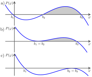
Figure 6: Example cubic potential curves for KdV traveling wave solutions: (a) periodic, (b) soliton, (c) constant. When $0<b_{3}-b_{2}\ll 1$, the periodic solution is approximately sinusoidal.

An alternative, mathematically motivated parameterization for $\varphi$ is to integrate eq. (2.35) twice and obtain the ODE

$$(\varphi_{\theta})^{2}=P(\varphi)\equiv\frac{1}{3k^{2}}(b_{1}-\varphi)(b_{2}-\varphi)(b_{3}-\varphi)\,,$$ (2.46)

where $b_{1}\leq b_{2}\leq b_{3}$, assumed real, are related to two constants of integration and the wavenumber $k$. As depicted in Fig. 6, the roots of the cubic potential $P(\varphi)$ determine the behavior of the traveling wave. All real solutions of interest satisfy $b_{2}\leq\varphi\leq b_{3}$. When two roots coalesce, the periodic solution degenerates to either a soliton when $b_{1}=b_{2}$ or a constant when $b_{2}=b_{3}$. For $0<b_{3}-b_{2}\ll 1$, the periodic solution is approximately sinusoidal. Averaging of the quantity $\mathcal{F}[\varphi]$ is therefore achieved via

$$\overline{\mathcal{F}[\varphi]}=\frac{1}{\pi}\int_{0}^{\pi}\mathcal{F}[\varphi(\theta)]\,\mathrm{d}\theta=\frac{1}{\pi}\int_{b_{2}}^{b_{3}}\frac{\mathcal{F}[\varphi]\,\mathrm{d}\varphi}{\sqrt{P(\varphi)}},$$ (2.47)

where derivatives of $\varphi(\theta)$ in $\mathcal{F}[\varphi]$ are replaced by $\sqrt{P(\varphi)}$. The $2\pi$-periodicity of $\varphi(\theta)$ implies on using (2.46) that

$$2\pi=\int^{2\pi}_{0}\,\mathrm{d}\theta=2\sqrt{3}k\int^{b_{3}}_{b_{2}}\frac{\,\mathrm{d}\varphi}{\sqrt{(b_{1}-\varphi)(b_{2}-\varphi)(b_{3}-\varphi)}},$$ (2.48)

which relates the wavenumber $k$ with the roots $\{b_{i}\}_{i=1}^{3}$ of the cubic (2.46).

The roots $\{b_{i}\}_{i=1}^{3}$ of the cubic (2.46) can be used as modulation variables in eqs. (2.43), (2.44), and (2.45) rather than the physical parameterization $\{k,a,\overline{\varphi}\}$. The two are related via

$$\begin{split}a&=b_{3}-b_{2},\\ k&=\frac{\pi\sqrt{b_{3}-b_{1}}}{2\sqrt{3}K(m)},\quad m=\frac{b_{3}-b_{2}}{b_{3}-b_{1}},\\ \overline{\varphi}&=b_{1}+(b_{3}-b_{1})\frac{E(m)}{K(m)},\end{split}$$ (2.49)

where $K(m)$ and $E(m)$ are the complete elliptic integrals of the first and second kind, respectively. The modulation solution of eqs. (2.43)–(2.45) determine the evolution of the slowly varying periodic solution of eq. (2.46), which is

$$\varphi(\theta)=b_{1}+(b_{3}-b_{1})\mathrm{dn}^{2}\left(\frac{K(m)}{\pi}\theta;m\right),$$ (2.50)

where $\mathrm{dn}$ is a Jacobi elliptic function and $m$ is defined in eq. (2.49).

In his 1965 paper [48], Whitham made an important discovery: using ingenious algebraic manipulations (see [54] for detail), he showed that the modulation system (2.43)–(2.45) for the KdV equation can be represented in Riemann invariant form

$$\frac{\partial r_{i}}{\partial T}+V_{i}\frac{\partial r_{i}}{\partial X}=0,\quad i=1,2,3\,.$$ (2.51)

The Riemann invariants $r_{1}\leq r_{2}\leq r_{3}$ found by Whitham are related to the roots of the potential curve according to

$$r_{1}=\frac{b_{1}+b_{2}}{2},\ \ r_{2}=\frac{b_{1}+b_{3}}{2},\ \ r_{3}=\frac{b_{2}+b_{3}}{2},\$$ (2.52)

while the characteristic velocities are expressed in terms of $r_{j}$ by

$$\begin{split}V_{1}&=V-\frac{2}{3}(r_{2}-r_{1})\frac{K(m)}{K(m)-E(m)}\\ V_{2}&=V-\frac{2}{3}(r_{2}-r_{1})\frac{(1-m)K(m)}{E(m)-(1-m)K(m)}\\ V_{3}&=V+\frac{2}{3}(r_{3}-r_{1})\frac{(1-m)K(m)}{E(m)},\end{split}$$ (2.53)

where $m=(r_{2}-r_{1})/(r_{3}-r_{1})$. The phase velocity is $V\equiv\omega/k=\frac{1}{3}(r_{1}+r_{2}+r_{3})$.

It will be convenient for the study of DSWs to identify the invertible transformation between the physical parametrization $(a,k,\overline{\varphi})$ and the Riemann invariants $(r_{1},r_{2},r_{3})$:

$$\begin{split}a&=2(r_{2}-r_{1}),\\ k&=\frac{\pi\sqrt{r_{3}-r_{1}}}{\sqrt{6}K(m)},\quad m=\frac{r_{2}-r_{1}}{r_{3}-r_{1}},\\ \overline{\varphi}&=r_{1}+r_{2}-r_{3}+2(r_{3}-r_{1})\frac{E(m)}{K(m)}.\end{split}$$ (2.54)

The periodic wave (2.50) takes the form

$$\varphi(\theta)=r_{1}+r_{2}-r_{3}+2(r_{3}-r_{1})\mathrm{dn}^{2}\left(\frac{K(m)}{\pi}\theta;m\right).$$ (2.55)

In the limit $r_{2}\to r_{3}$ ($m\to 1$) (cf. Fig. 6b), the wave (2.55) takes the form of a soliton

$$\varphi=\overline{\varphi}+a_{\rm s}\mathrm{sech}^{2}\left(\frac{\sqrt{a_{\rm s}}}{\sqrt{12}}(x-V_{\rm s}t-\theta_{0})\right),$$ (2.56)

where $V_{\rm s}=\overline{\varphi}+a_{\rm s}/3$ is the soliton amplitude-speed relation. The background $\overline{\varphi}$, soliton amplitude $a_{\rm s}$, and velocity $V_{\rm s}$ are expressed in terms of $r_{1}$ and $r_{3}$ as

$$\overline{\varphi}=r_{1},\quad a_{\rm s}=2(r_{3}-r_{1}),\quad V_{\rm s}=\frac{1}{3}(r_{1}+2r_{3}).$$ (2.57)

In the limit $r_{2}\to r_{1}$ ($m\to 0$) (cf. Fig. 6c), the wave (2.55) is a vanishing harmonic wave

$$\varphi=\overline{\varphi}+\frac{a_{\rm h}}{2}\left(\cos(kx-\omega_{0}t)-1\right)+\mathcal{O}(a_{\rm h}^{2}),$$ (2.58)

where $\omega_{0}(k,\overline{\varphi})=\overline{\varphi}k-k^{3}$ is the linear dispersion relation. The wave amplitude $a_{\rm h}$, wavenumber $k$, and background $\overline{\varphi}$ are related to the Riemann invariants via

$$\overline{\varphi}=r_{3},\quad a_{\rm h}=2(r_{2}-r_{1})\ll 1,\quad k^{2}=\frac{2}{3}(r_{3}-r_{1}).$$ (2.59)

A convenient and compact representation of the characteristic velocities (2.53) can be obtained by considering the wave conservation equation (2.45) as a consequence of the diagonal system (2.51) [73, 74, 54]. Equations (2.51) imply that $k_{T}+\omega_{X}=0$ can be written as (recall $\partial_{j}=\partial/\partial r_{j}$)

$$\sum_{j=1}^{3}\frac{\partial r_{j}}{\partial X}\left[-V_{j}\partial_{j}k+\partial_{j}\omega\right]=0.$$

Generic variations of $r_{j}$ imply that each expression in brackets must be zero so that the characteristic velocities satisfy

$$V_{j}=\frac{\partial_{j}\omega}{\partial_{j}k}=\left(1-\frac{L}{\partial_{j}L}\partial_{j}\right)V,\quad i=1,2,3,$$ (2.60)

where $L=2\pi/k=2K(m)\sqrt{6/(r_{3}-r_{1})}$, and the relation $\omega=kV$ was used. We note that expressions (2.60) are universal for diagonalizable modulation systems and elucidate the significance of the characteristic velocities $V_{j}$ of the Whitham modulation system as nonlinear group velocities.

We introduced the small parameter $\varepsilon$ and the slow variables $X$ and $T$ in order to clearly implement the multiple scales perturbation procedure. This is a standard approach for limit process expansions (see, e.g., [75]). What is effectively being considered is the long time behavior of the modulated periodic wave. Now that we know the Whitham modulation equations (2.51), rather than explicitly identifying the small parameter $\varepsilon$, we can take $\varepsilon=1$ with the caveat that the modulation equations are valid over long time and spatial scales, $t,x\gg 1$.

An alternative derivation method and properties of the KdV Whitham system in Riemann invariant form (2.51) will be described in subsequent sections.

2.2.3 Whitham vs. NLS

The Whitham equations, a system of quasi-linear equations of hydrodynamic type, are applicable to modulations of large amplitude dispersive waves. The structure of slowly varying, weakly nonlinear, nearly monochromatic wavetrains is governed by the NLS equation, a universal model of this phenomenon [76]. It is natural to ask how these two models are related. Newell [77] explored this issue with a specific model equation but the ideas are applicable more generally [72].

An obvious difference between the NLS and Whitham equations is that the former is dispersive and the latter is not. Therefore, taking a straightforward, small amplitude reduction of the Whitham equations will not result in NLS. Consider the derivation via multiple scales of the KdV Whitham equations in the previous section. The two secularity conditions at first order (2.43), (2.44) result from orthogonality to the two-dimensional kernel of the adjoint linear operator $\mathcal{A}^{\dagger}$ (2.40) (recall that only $w_{1}$, $w_{2}$ in (2.41) are $2\pi$-periodic, while $w_{3}$ is not). This enabled the maintenance of a well-ordered, uniform asymptotic sequence as $\varepsilon\to 0$. In the weakly nonlinear regime, we have $\varphi=\overline{\varphi}+\frac{a}{2}\cos(\theta)+\mathcal{O}(a^{2})$ so that, with $\theta_{0}=\pi/2$ in eq. (2.41),

$$w_{3}(\theta)=\frac{2}{a}(-1+\sin\theta)+\mathcal{O}(1),\quad 0<a\ll 1,$$

a $2\pi$-periodic function, linearly independent of $w_{1}$ and $w_{2}$. Now the operator $\mathcal{A}^{\dagger}$ admits a three-dimensional kernel so an additional orthogonality condition is required to remove secularity. Therefore, it is not possible to first take the asymptotic limit process $\varepsilon\to 0$ and then $a\to 0$. The derivation of NLS relies on the maximal balance $\varepsilon=\mathcal{O}(a)$ and a time scale $\varepsilon^{2}t$ and spatial scale $\varepsilon(x-c_{\rm g}t)$ where $c_{\rm g}$ is the group velocity of linear waves. Therefore, before taking the small amplitude reduction, higher order corrections to the Whitham equations (2.43) and (2.44) must be included. They include dispersive effects. See [1], where Whitham incorporated dispersive effects into the modulation equations for the nonlinear Klein-Gordon equation. More recently, the emergence of dispersion in modulations of a general class of second order equations has been investigated in [78].

2.2.4 IST- integrability and Riemann invariants

After Whitham’s discovery of the diagonal structure of the KdV modulation system, a similar set of Riemann invariants was found in [79] for the modified KdV (mKdV) equation, connected with the KdV equation by the Miura transformation [80]. Later, Flaschka, Forest and McLaughlin (FFM) [61] showed that the availability of Riemann invariants for the KdV-Whitham system is intimately linked to the integrable structure of the KdV equation via the IST. Subsequently, Riemann invariants were found for other modulation systems associated with integrable equations such as the nonlinear Schrödinger equation [81, 82], the Kaup-Boussinesq system [83] and others.

The method of FFM is based on finite-gap integration theory, a highly non-trivial extension of the IST utilizing tools from algebraic-geometry to the case of periodic boundary conditions (see [84]). Finite-gap theory was used in [61] to prescribe and study equations for the slow modulations of $N$-phase wavetrains via averaging of conservation laws over the $N$-torus. Note that Whitham’s original paper [48] considered only $N=1$. The main result of [61] is that the Riemann invariants of the KdV-Whitham modulation system are the endpoints of spectral bands of $N$-phase or, alternatively, $N$-gap KdV solutions. Krichever [85] generalized the FFM construction to the two-dimensional case in the KP equation and also derived a family of exact solutions to the modulation equations.

The FFM construction of multiphase averaging is quite technical and makes prominent use of the theory of hyperelliptic Riemann surfaces and associated Abelian differentials. For the single-phase case, playing a key role in DSW theory, Kamchatnov [86, 54] developed a reduced version of the finite-gap averaging technique, which does not require the use of algebro-geometric tools of FFM theory. Kamchatnov’s method applies to integrable equations belonging to the Ablowitz-Kaup-Newell-Segur (AKNS) hierarchy [87] and has the advantage of delivering both the traveling wave solution and the Whitham equations in the Riemann invariant parametrization. We now apply this method to recover the Riemann invariant form (2.51) of the KdV-Whitham system.

We shall be using here the “IST-friendly” normalization of the KdV equation

$$u_{t}+6uu_{x}+u_{xxx}=0.$$ (2.61)

The integrability of the KdV equation is based on the possibility of representing it as a compatibility condition of two linear differential equations, called the Lax pair, for the same complex function $\psi(x,t)$ [88]. It is convenient to represent the KdV Lax pair in the form

$$\psi_{xx} =\mathcal{A}\psi,$$ (2.62)

$$\psi_{t} =-\frac{1}{2}\mathcal{B}_{x}\psi+\mathcal{B}\psi_{x},$$ (2.63)

where

$$\mathcal{A}=-(u+\lambda),\quad\mathcal{B}=4\lambda-2u,$$ (2.64)

and $\lambda$ is a complex parameter. The first equation (2.62) is the quantum-mechanical Schrödinger equation
$-\psi_{xx}+V(x)\psi=\lambda\psi$, which specifies for a given potential $V(x)=-u(x,t)$ a stationary spectral problem with $t$ being a parameter. The second equation (2.63) of the Lax pair constitutes the evolution problem for $\psi$. A calculation shows that the compatibility condition $(\psi_{xx})_{t}=(\psi_{t})_{xx}$ yields the KdV equation (2.61) provided the isospectrality condition $\lambda_{t}=0$ holds.

We now take two basis solutions $\psi^{+}$ and $\psi^{-}$ of (2.62) with the asymptotic behaviors $\psi^{\pm}\sim e^{\pm i\sqrt{\lambda}x}$ for $\lambda\gg 1$ and construct the squared basis function

$$g=\psi^{+}\psi^{-}.$$

It is possible to show that the function $g(\lambda,x,t)$ satisfies the equations

$$g_{xxx}-2\mathcal{A}_{x}g-4\mathcal{A}g_{x}=0,$$ (2.65)

$$g_{t}=\mathcal{B}g_{x}-\mathcal{B}_{x}g\,,$$ (2.66)

equivalent to the Lax pair (2.62), (2.63). Equation (2.66) can be rewritten in the conservative form

$$\left(\frac{1}{g}\right)_{t}=\left(\frac{\mathcal{B}}{g}\right)_{x}$$ (2.67)

provided $g\neq 0$. This expression generates an infinite series, each term a distinct KdV conservation law, by expansion of (2.67) in powers of $1/\lambda$ (see [54] for details).

Multiplying (2.65) by $g$ and integrating once yields

$$\frac{1}{2}gg_{xx}-\frac{1}{4}g_{x}^{2}-\mathcal{A}g^{2}=R(\lambda),$$ (2.68)

where $R(\lambda)$ is the integration constant, which can be a function of the spectral parameter $\lambda$ and, in principle, a function of $t$.

The crucial step in Kamchatnov’s method is the identification of the function $R(\lambda)$ with the third degree polynomial defining, via the radical $\sqrt{R(\lambda)}$, the elliptic Riemann surface on which periodic KdV solutions exist. To this end, we assume

$$\begin{split}R(\lambda)=(\lambda-\lambda_{1})(\lambda-\lambda_{2})(\lambda-\lambda_{3})\\ =\lambda^{3}-s_{1}\lambda^{2}+s_{2}\lambda-s_{3},\end{split}$$ (2.69)

where $\lambda_{1}\leq\lambda_{2}\leq\lambda_{3}$ are constants, and

$$\left.\begin{split}s_{1}&=\lambda_{1}+\lambda_{2}+\lambda_{3},\\ s_{2}&=\lambda_{1}\lambda_{2}+\lambda_{1}\lambda_{3}+\lambda_{2}\lambda_{3},\\ s_{3}&=\lambda_{1}\lambda_{2}\lambda_{3}\end{split}\qquad\right\}$$ (2.70)

are elementary symmetric polynomials. In what follows, we will show that the dependence (2.69) indeed delivers the periodic solution $u(x,t)$. We also note that in the general framework of finite-gap theory (see, e.g., [89]) the roots $\lambda_{j}$ of the polynomial (2.69) represent the endpoints of the spectral bands of the Schrödinger operator (2.62) with the potential given by the periodic KdV solution.

The structure of equation (2.68) suggests that its solution $g(\lambda,x,t)$ can be sought in the form of a first degree polynomial in $\lambda$,

$$g=\lambda-\mu(x,t),$$ (2.71)

where $\mu(x,t)$ is a new unknown function called the auxiliary spectrum. Substituting (2.71), (2.69) into (2.68), we obtain

$$\begin{split}-\frac{1}{2}(\lambda-\mu)\mu_{xx}-\frac{1}{4}\mu_{x}^{2}+(u+\lambda)(\lambda-\mu)^{2}=\\ \lambda^{3}-s_{1}\lambda^{2}+s_{2}\lambda-s_{3}.\end{split}$$ (2.72)

Equating the coefficients of $\lambda^{2}$ on both sides yields

$$u(x,t)=2\mu-s_{1}\,.$$ (2.73)

Next, after substitution of (2.71) into (2.66), we obtain

$$\mu_{t}=(4\lambda-2u)\mu_{x}+2(\mu-\lambda)u_{x}.$$ (2.74)

Setting the free spectral parameter $\lambda=\mu$ in (2.72) and (2.74), which can be done at any point $(x,t)=(x_{0},t_{0})$, we obtain:

$$\mu_{x}=2\sqrt{-R(\mu)},\quad\mu_{t}=-2s_{1}\mu_{x}.$$ (2.75)

The second equation (2.75) implies $\mu=\mu(\xi)$, where $\xi=x-Vt+\xi_{0}$ is the traveling phase with the phase velocity

$$V=-2s_{1}=-2(\lambda_{1}+\lambda_{2}+\lambda_{3}),$$ (2.76)

and $\xi_{0}$ is an arbitrary initial phase.

Now, the first ODE (2.75) becomes

$$\mu_{\xi}=2\sqrt{-R(\mu)}$$ (2.77)

implying that real-valued $\mu$ oscillates between $\lambda_{2}$ and $\lambda_{3}$. Integrating (2.77), we obtain the elliptic (cnoidal wave) solution of the KdV equation, parametrized by the spectral branch points $\lambda_{1},\lambda_{2},\lambda_{3}$:

$$u(x,t)=\lambda_{3}-\lambda_{1}-\lambda_{2}-2(\lambda_{3}-\lambda_{2})\textrm{sn}^{2}(\sqrt{\lambda_{3}-\lambda_{1}}\xi,m),$$ (2.78)

where the modulus $m=(\lambda_{3}-\lambda_{2})/(\lambda_{3}-\lambda_{1})$.

The wavelength of (2.78), which is the period of the nonlinear oscillator (2.77), is

$$L=\int\limits^{L}_{0}d\xi=\int\limits_{\lambda_{2}}^{\lambda_{3}}\frac{\,\mathrm{d}\mu}{\sqrt{-R(\mu)}}.$$ (2.79)

We now recall that the direct computation of the periodic solution via substituting the ansatz $u=\phi(\xi)$ into the KdV equation (2.61) yields (see (2.46), where $\theta=k\xi$ with $k=2\pi/L$)

$$\begin{split}\phi_{\xi}^{2}=2(b_{1}-\phi)(b_{2}-\phi)(b_{3}-\phi)\equiv-Q(\phi),\\ V=2(b_{1}+b_{2}+b_{3}),\quad b_{1}\leq b_{2}\leq b_{3}\,.\end{split}$$ (2.80)

Using (2.73), (2.75) we obtain $\phi(\xi)=2\mu(\xi)-s_{1}$. Substituting this into (2.80) we obtain $Q(2\mu+V/2)=16R(\mu)$, which after some algebra yields the relations between the roots $\lambda_{1},\lambda_{2},\lambda_{3}$ of the spectral polynomial $R(\lambda)$ and the roots $b_{1},b_{2},b_{3}$ of the potential curve $Q(\phi)$ (cf. (2.52))

$$\lambda_{1}=-\frac{b_{2}+b_{3}}{2};\ \ \lambda_{2}=-\frac{b_{1}+b_{3}}{2},\ \ \lambda_{3}=-\frac{b_{1}+b_{2}}{2}.$$ (2.81)

We now introduce slow modulations of the periodic solution (2.78) via $\lambda_{j}(X,T)$, $X=\varepsilon x$, $T=\varepsilon t$, $\varepsilon\ll 1$, and derive modulation equations for $\{\lambda_{j}\}_{j=1}^{3}$ using the Kamchatnov adaptation of the FFM-Whitham averaging procedure, which, instead of averaging the necessary number of conservation laws (2.43), (2.44), one averages all KdV conservation laws via the generating equation (2.67).

Before deriving the modulation equations, we represent the generating equation (2.67) in a form suitable for averaging. From (2.68), it follows that $1/g$ is singular when $\lambda=\lambda_{j}$, $j=1,2,3$, which becomes apparent if one introduces the normalization

$$\hat{g}=g/\sqrt{R(\lambda)},$$ (2.82)

which reduces equation (2.68) to

$$\hat{g}\hat{g}_{xx}-(\hat{g}_{x})^{2}+(u+\lambda)\hat{g}^{2}=1,$$ (2.83)

so that $\hat{g}$ does not have singularities at $\lambda=\lambda_{j}$. Thus, to remove the singularities at $\lambda=\lambda_{j}$ in (2.67) we multiply it by $\sqrt{R(\lambda)}$ and use (2.71), (2.73) to obtain the normalized generating equation

$$\left[\sqrt{R(\lambda)}\cdot\frac{1}{\lambda-\mu}\right]_{t}+\left[\sqrt{R(\lambda)}\cdot\left(-4-\frac{2s_{1}}{\lambda-\mu}\right)\right]_{x}=0.$$ (2.84)

We now consider the slowly modulated cnoidal wave (2.78) by assuming $\lambda_{j}=\lambda_{j}(X,T)$. Introducing a period-average of (2.77) by (cf. (2.47))

$$\langle{\mathcal{F}[\mu]}\rangle=\frac{1}{L}\int_{0}^{L}\mathcal{F}[\mu(\xi)]\,\mathrm{d}\xi=\frac{1}{L}\int_{\lambda_{2}}^{\lambda_{3}}\frac{\mathcal{F}[\mu]\,\mathrm{d}\mu}{\sqrt{-R(\mu)}},$$

we apply it to (2.84) to obtain the generating equation for the modulation equations

$$\left[\sqrt{R(\lambda)}\Big{\langle}\frac{1}{\lambda-\mu}\Big{\rangle}\right]_{T}$$

$$+\left[\sqrt{R(\lambda)}\left(-4-2s_{1}\Big{\langle}\frac{1}{\lambda-\mu}\Big{\rangle}\right)\right]_{X}=0.$$ (2.85)

We now observe that differentiation of $\sqrt{R({\lambda})}$ in (2.85) yields the factors

$$\frac{1}{\sqrt{\lambda-\lambda_{j}}}\frac{\partial\lambda_{j}}{\partial T}\qquad\textrm{and}\qquad\frac{1}{\sqrt{\lambda-\lambda_{j}}}\frac{\partial\lambda_{j}}{\partial X},$$

which are singular as $\lambda\rightarrow\lambda_{j}$. We then multiply (2.85) by $\sqrt{\lambda-\lambda_{j}}$ and take the limit $\lambda\to\lambda_{j}$ to obtain

$$\frac{\partial\lambda_{j}}{\partial T}+v_{j}\frac{\partial\lambda_{j}}{\partial X}=0,\ \ j=1,2,3,$$ (2.86)

where

$$v_{j}=-2s_{1}-\frac{4}{\big{\langle}\frac{1}{\lambda_{j}-\mu}\big{\rangle}}\,.$$ (2.87)

Thus $\lambda_{j}$ are the Riemann invariants of the modulation system (2.86). Computing the characteristic velocities (2.87), we arrive at the expressions (2.53), where $V_{j}({\bf r})=v_{j}(\boldsymbol{\lambda}(\bf r))$ and

$$r_{1}=-6\lambda_{3},\quad r_{2}=-6\lambda_{2},\quad r_{3}=-6\lambda_{1}\,.$$ (2.88)

2.2.5 Properties of the KdV-Whitham system

Direct verification shows that the KdV-Whitham system (2.51), (2.53) is: (i) strictly hyperbolic (2.10); (ii) genuinely nonlinear (2.11); (iii) semi-Hamiltonian (2.23). The first two properties imply the existence of simple wave solutions (see Sec. 2.1), and the third one implies integrability of the KdV-Whitham system via the generalized hodograph transform (2.24). We note that the general proof of strict hyperbolicity for the multiphase averaged KdV-Whitham system was carried out by Levermore [90]. Integrability of the KdV-Whitham system was proved by Tsarev [62]. Generally, one can talk about the “preservation of integrability when averaging” principle [60].

Of particular interest are two limits of the KdV-Whitham system (2.51), (2.53) corresponding to the harmonic and soliton limits of the traveling wave (2.50). In the harmonic limit, the modulus $m=0$ (i.e. $r_{2}=r_{1}$) and the characteristic velocities $V_{2}$ and $V_{1}$ merge together

$$m=0:\ \ V_{2}(r_{1},r_{1},r_{3})=V_{1}(r_{1},r_{1},r_{3})=-r_{3}+2r_{1}\,.$$ (2.89)

One can also show that in this limit, the velocity $V_{3}(r_{1},r_{1},r_{3})=r_{3}$. Thus, in the harmonic limit $m=0$, the Whitham system (2.51), (2.53) reduces to a system of two equations,

$$\frac{\partial r_{1}}{\partial T}+(2r_{1}-r_{3})\frac{\partial r_{1}}{\partial X}=0,\ \ \frac{\partial r_{3}}{\partial T}+r_{3}\frac{\partial r_{3}}{\partial X}=0.$$ (2.90)

The second equation in (2.90) is the dispersionless KdV or Hopf equation $u_{T}+uu_{X}=0$ for $u=r_{3}$.

In the opposite, soliton limit $m=1$ (i.e. $r_{2}=r_{3}$), there is a similar degeneracy, but now the merged characteristic velocities are $V_{2}$ and $V_{3}$

$$m=1:\ \ V_{2}(r_{1},r_{3},r_{3})=V_{3}(r_{1},r_{3},r_{3})=\frac{1}{3}(2r_{3}+r_{1})\,,$$ (2.91)

while the remaining velocity $V_{1}(r_{1},r_{3},r_{3})=r_{1}$ yields the Hopf equation for $r_{1}$. Therefore, the soliton reduction of the KdV-Whitham system is

$$\frac{\partial r_{3}}{\partial T}+\frac{1}{3}(2r_{3}+r_{1})\frac{\partial r_{3}}{\partial X}=0,\ \ \frac{\partial r_{1}}{\partial T}+r_{1}\frac{\partial r_{1}}{\partial X}=0.$$ (2.92)

It is instructive to note that the merged characteristic velocities (2.89) and (2.91) in the harmonic and soliton limits, respectively, define a regular characteristic because the order of the modulation system reduces from three to two in both limits. Strict hyperbolicity and genuine nonlinearity of the modulation system are preserved in these limits.

We conclude this section with one more important property of the KdV-Whitham equations: the characteristic velocities (2.53) are homogeneous functions of ${\bf r}$ (i.e. $V_{j}(C{\bf r})=C^{\alpha}V_{j}({\bf r})\ \hbox{for all}\ C>0$) with homogeneity degree $\alpha=1$. This property defines the symmetry

$${\bf r}\to C{\bf r},\quad T\to C^{2}T,\quad X\to C^{3}X,$$ (2.93)

where $C=\hbox{const}$. The invariant scaling (2.93) of (2.51), (2.53) along with the hydrodynamic symmetry

$$X\to CX,\quad T\to CT$$ (2.94)

of all quasi-linear equations give rise to two special families of similarity modulation solutions. These families describe two fundamental classes of DSWs described in Secs. 3.1 and 3.2.3 below.

2.2.6 General solution of the KdV-Whitham equations

The strict hyperbolicity and genuine nonlinearity properties of the KdV-Whitham system guarantee the existence of three families of simple wave solutions, which can be readily constructed using characteristics. In these solutions, only one Riemann invariant is changing while the other two are constant (see Sec. 2.1.2). More general solutions are given by the generalized hodograph formulae (2.21), which requires solving an overdetermined system of linear PDEs (2.22) due to Tsarev [62] in order to find the functions $W_{j}$, $j=1,2,3$. Despite linearity, the coefficients in (2.22) involve rather complex combinations of complete elliptic integrals (see (2.53)), so their integration using standard methods is not feasible.

We shall take advantage of the nonlinear group velocity representation (2.60) for the characteristic velocities $V_{j}=(1-\frac{L}{\partial_{j}L}\partial_{j})V$ where $V=\frac{1}{3}(r_{1}+r_{2}+r_{3})$ is the phase velocity and the wavelength $L$ can be conveniently represented as a loop integral

$$L=\sqrt{\tfrac{3}{2}}\oint\frac{\,\mathrm{d}\lambda}{\sqrt{(\lambda-r_{1})(r_{2}-\lambda)(r_{3}-\lambda)}}.$$ (2.95)

The contour of integration surrounds clockwise the branchcut between $r_{1}$ and $r_{2}$ on the upper sheet of the elliptic Riemann surface of the radical $\sqrt{(\lambda-r_{1})(\lambda-r_{2})(\lambda-r_{3})}$.

Substituting (2.60) into the Tsarev equations (2.25) and using $\partial_{ij}\omega=\partial_{ji}\omega$, we obtain the relationship

$$\partial_{j}(\partial_{i}kW_{i})=\partial_{i}(\partial_{j}kW_{j})\,.$$ (2.96)

This analogue of a curl-free condition implies the existence of a scalar function $q(r_{1},r_{2},r_{3})$ so that (cf. (2.60))

$$W_{j}=\frac{\partial_{j}(kq)}{\partial_{j}k}=\left(1-\frac{L}{\partial_{j}L}\partial_{j}\right)q,\quad j=1,2,3.$$ (2.97)

The integration of the Tsarev equations (2.25) for the vector $(W_{1},W_{2},W_{3})$ is then reduced to finding a single scalar potential function $q({\bf r})$. To obtain the equation for $q$, we substitute (2.60) and (2.97) into (2.25) and, using the loop integral representation (2.95), obtain the overdetermined system of six Euler-Poisson-Darboux (EPD) equations in the three-dimensional space of Riemann invariants

$$\begin{split}2(r_{i}-r_{j})\frac{\partial^{2}q}{\partial r_{i}\partial r_{j}}=\frac{\partial q}{\partial r_{i}}-\frac{\partial q}{\partial r_{j}}\,,\\ \\ i,j=1,2,3;\quad i\neq j\,.\end{split}$$ (2.98)

Each of the equations in (2.98) for a given pair $(r_{i},r_{j})$ represents a particular case of the classical EPD equation appearing, in particular, in the theory of surfaces [91], gas dynamics [92] and the theory of colliding gravitational waves [93]. The system (2.98) appears in the classical differential geometry study [94] by Eisenhart.

A calculation of the mixed third derivatives shows that the system (2.98) is compatible, which also proves the semi-Hamiltonian property (2.23) and integrability of the KdV-Whitham system (2.51).

Summarizing, the mapping between EPD system solutions $q(r_{1},r_{2},r_{3})$ and solutions of the KdV-Whitham system (2.51) has the form

$$x-V_{j}t=\left(1-\frac{L}{\partial_{j}L}\partial_{j}\right)q,\quad j=1,2,3.$$ (2.99)

Importantly, all non-constant and non-singular local solutions of the modulation system (2.51) can be obtained in this way. The transformation (2.99) was found independently in [73, 95, 96].

Direct verification shows that the function

$$G(\lambda;r_{1},r_{2},r_{3})=\frac{\Phi(\lambda)}{\sqrt{(\lambda-r_{1})(\lambda-r_{2})(\lambda-r_{3})}},$$ (2.100)

where $\Phi(\lambda)$ is an arbitrary function, satisfies the EPD system for any $\lambda$, i.e. $G$ represents the generating function for solutions of the EPD system (2.98) and, consequently via (2.99), for the solutions to the Whitham-KdV equations (2.51). In particular, choosing $\Phi(\lambda)=\lambda^{3/2}$ and expanding the generating function $G(\lambda,r_{1},r_{2},r_{3})$ for $\lambda\gg 1$, we obtain

$$G=1+\frac{q_{1}}{\lambda}+\frac{q_{2}}{\lambda^{2}}+\dots,$$ (2.101)

where

$$\begin{split}q_{1}&=2s_{1}\,,\ \ q_{2}=6s_{1}^{2}-8s_{2},\\ q_{3}&=5s_{1}^{3}-12s_{1}s_{2}+8s_{3},\ \dots,\end{split}$$ (2.102)

and $s_{1},s_{2},s_{3}$ are the elementary symmetric polynomials of $r_{1},r_{2},r_{3}$ (recall (2.70)). Each $q_{\alpha}({\bf r})$, $\alpha=1,2,3,\dots$ is a symmetric homogeneous function of $r_{1},r_{2},r_{3}$ with homogeneity degree $\alpha$ satisfying the EPD system (2.98). This family of homogeneous modulation solutions of the EPD system was first obtained by Krichever [85] utilizing an algebro-geometric approach to the integration of the multiphase KdV-Whitham equations. Since the characteristic velocities $V_{j}$ are homogeneous functions of ${\bf r}$ with the homogeneity degree $1$, it is not difficult to show that the homogeneous solutions $q_{\alpha}({\bf r})$ of the EPD system give rise, via the mapping (2.99), to the generalized similarity (scaling) modulation solutions [49, 85],

$$r_{j}=t^{\gamma}R_{j}(\frac{x}{t^{\gamma+1}})\,,\quad\gamma=\frac{1}{\alpha-1}\,\quad j=1,2,3$$ (2.103)

for $\alpha\neq 1$. The general solution of (2.98) is parametrized by three functions of a single variable, as is the solution to the Tsarev equations (2.25) for $(W_{1},W_{2},W_{3})$. Then, using the generating function (2.100), one obtains the general solution to the EPD system (2.98) [94]

$$q(r_{1},r_{2},r_{3})=\sum\limits_{j=1}^{3}\int\limits^{r_{j}}_{0}\frac{\Phi_{j}(\lambda)}{\sqrt{(\lambda-r_{1})(\lambda-r_{2})(\lambda-r_{3})}}\,\mathrm{d}\lambda,$$ (2.104)

where $\Phi_{j}(\lambda),\ j=1,2,3$ are arbitrary complex functions.

2.2.7 Modulation phase shift

We now describe an important connection between solutions of the EPD system (2.98) and the phase of the slowly modulated periodic solution of the KdV equation. The phase appears in the modulation construction in two ways. In the derivation of the modulation equations via multiple-scale WKB-type expansions described in Sec. 2.2.2, the generalized phase $\theta$ is determined by the modulation solution via the local wavenumber and local frequency, which are defined as $k=\theta_{x}=\varepsilon\theta_{X}$ and $\omega=-\theta_{t}=-\varepsilon\theta_{T}$ respectively [1]. On the other hand, the IST based finite-gap approach to the derivation of the modulation equations described in Sec. 2.2.4 yields the explicit expression $\theta=k\xi=kx-\omega t+\theta_{0}$ for the phase. These two definitions of the phase are equivalent for the non-modulated periodic solution, but the presence of slow modulations imposes some constraints on the initial phase $\theta_{0}$, which can be viewed as a phase shift due to modulation. To find this phase correction, we first represent the phase in the form $\theta=\varepsilon^{-1}(kX-\omega T+\Theta_{0})$ where $\Theta_{0}=\varepsilon\theta_{0}$. In the modulated wave, $\Theta_{0}$ undergoes slow spatiotemporal variations, so it is natural to assume that $\Theta_{0}(X,T)=\Upsilon({\bf r}(X,T))$. The modulation phase shift function $\Upsilon({\bf r})$ is then found from the definition of the local wavenumber

$$k=\varepsilon\theta_{X}=k+\sum\limits_{j=1}^{3}\left\{\frac{\partial k}{\partial r_{j}}X-\frac{\partial\omega}{\partial r_{j}}T+\frac{\partial\Upsilon}{\partial r_{j}}\right\}\frac{\partial r_{j}}{\partial X},$$ (2.105)

which yields

$$\sum\limits_{j=1}^{3}\left\{\frac{\partial k}{\partial r_{j}}X-\frac{\partial\omega}{\partial r_{j}}T+\frac{\partial\Upsilon}{\partial r_{j}}\right\}\frac{\partial r_{j}}{\partial X}=0\,.$$ (2.106)

Since equation (2.106) must be valid for all non-constant solutions $r_{j}(X,T)$, each expression in brackets must vanish and we have

$$\frac{\partial k}{\partial r_{j}}X-\frac{\partial\omega}{\partial r_{j}}T+\frac{\partial\Upsilon}{\partial r_{j}}=0,\quad j=1,2,3,$$ (2.107)

provided $(r_{j})_{X}\neq 0$ for all $j$. We note that using the local frequency definition instead of the wavenumber for the determination of the phase correction leads to the same expression (2.107). Dividing (2.107) by $\frac{\partial k}{\partial r_{j}}$ and using (2.60), we obtain

$$X-V_{j}T=\frac{\partial_{j}\Upsilon}{\partial_{j}k},\quad j=1,2,3.$$ (2.108)

Comparing (2.108) with the generalized hodograph solution (2.99), we find that $\Upsilon=kq({\bf r})+C$, where $C$ is an arbitrary constant, which can be set to zero without loss of generality. Thus, the phase correction $\theta_{0}$ in the modulated KdV solution is determined by the solution of the EPD equation. A particular form of this result was obtained in [97] by analyzing the expression for the phase in the rigorous asymptotic solution of the initial value problem for the semi-classical KdV equation obtained in [99]. Here, it is derived as a general property inherent within the modulation theory. We stress that the existence of the function $\Upsilon(\mathbf{r})$ is not obvious a priori. It is guaranteed only due to the semi-Hamiltonian structure of the KdV-Whitham system (i.e., to the consistency of the associated Tsarev system (2.25)), which is inherited from the integrability of the KdV equation. Thus, one can expect that the representation of the phase $\theta(x,t)$ of the modulated solution in the form $\theta=kx-\omega t+\varepsilon^{-1}\Theta_{0}(X,T)$ is only possible for integrable equations.

We now note that the phase compatibility condition (2.107) can be written as the stationary phase condition

$$\nabla_{\bf r}\theta=0\,.$$ (2.109)

Modulations of the periodic KdV solution are defined by the stationary point of the phase in the space of Riemann invariants of the Whitham system. Equation (2.109) has been derived for the general case of multiphase modulated KdV solutions in [98]. Along with the nonlinear extension (2.60) of the definition of the group velocity, the stationary phase condition (2.109) provides further striking parallels between modulation theories for linear and nonlinear waves [1]. We note that the precise meaning of the equivalence between the stationary phase condition and the modulation solution has been revealed by Deift, Venakides and Zhou [99] in the framework of the Riemann-Hilbert problem approach to the semi-classical IST for the KdV equation.

2.3 NLS-Whitham equations

2.3.1 NLS dispersive hydrodynamics

The cubic nonlinear Schrödinger equation

$$i\psi_{t}+\frac{1}{2}\psi_{xx}-\sigma|\psi|^{2}\psi=0,\quad\sigma=\pm 1\,,$$ (2.110)

is a particular case of the gNLS equation (1.4). Equation (2.110) models slow evolution of the normalized complex valued envelope of a nearly monochromatic, weakly nonlinear wave $\psi(x,t)e^{i(k_{0}x^{\prime}-\omega_{0}t^{\prime})}$, where $k_{0}$ and $\omega_{0}=\omega(k_{0})$ are the wavenumber and the frequency of the short-wavelength “carrier” wave respectively, $c_{\rm g}=\omega^{\prime}(k_{0})$ is the group velocity; the independent variables $x,t$ in the NLS equation (2.110) are related to physical space and time $x^{\prime},t^{\prime}$ as $x=\delta[x^{\prime}-c_{\rm g}t^{\prime}]$, $t=\delta^{2}t^{\prime}$, where $\delta\ll 1$ is the amplitude parameter.

Some of the prominent physical contexts for the NLS equation (2.110) are the dynamics of deep water waves ($\sigma=-1$), Langmuir waves in plasma ($\sigma=-1$), spin waves in a ferromagnet ($\sigma=\pm 1$), and electromagnetic waves in a nonlinear, defocusing ($\sigma=1$) or focusing ($\sigma=-1$) medium, notably in nonlinear optics. It also models the dynamics of a geometrically constrained Bose-Einstein condensate (BEC) in the mean-field approximation (both signs of $\sigma$ are relevant). Note that in the BEC context, the derivation of the NLS equation (termed the Gross-Pitaevskii equation, see (3.59) below) is not a slowly varying envelope approximation but rather a direct approximation of the condensate order parameter.

From the mathematical point of view, the NLS equation (2.110), similar to the KdV equation (2.33), is a universal [76], integrable nonlinear dispersive equation. Using the Madelung transformation $\psi\mapsto(\rho,u)$ (1.5), where $\rho(x,t)>0$ and $u(x,t)$ are real-valued functions, we can exactly represent the NLS equation (2.110) in the dispersive-hydrodynamic form (1.1)

$$\begin{split}\rho_{t}+(\rho u)_{x}&=0,\\ (\rho u)_{t}+(\rho u^{2}+\frac{\sigma}{2}\rho^{2})_{x}&=\frac{1}{4}(\rho(\log\rho)_{xx})_{x}\,,\end{split}$$ (2.111)

with the fluid-like density $\rho$, velocity $u$, and pressure

$$P(\rho)=\frac{\sigma}{2}\rho^{2}.$$ (2.112)

The dispersionless, long-wave limit of the system (2.111) is obtained by neglecting the right-hand side of the momentum equation (2.111). With some manipulation, the dispersionless equations can be written

$$\rho_{t}+(\rho u)_{x}=0,\quad u_{t}+(\rho u^{2}+\frac{\sigma}{2}\rho^{2})_{x}=0\,.$$ (2.113)

The system (2.113) is hyperbolic for $\sigma=1$ and elliptic for $\sigma=-1$. The latter implies ill-posedness of the Cauchy problem for all but analytic initial data. This can be interpreted in the context of the pressure law (2.112) where $\sigma=-1$ coincides with a negative pressure and an attractive interaction. In nonlinear optics, this effect corresponds to focusing of the optical signal. When $\sigma=-1$, a slightly perturbed, uniform density evolving according to (2.111) will experience modulational instability [71], thus the hydrodynamic background is unstable. When $\sigma=1$, the pressure (2.112) is positive, resulting in a repulsive or defocusing interaction. In this case, a uniform density solution to (2.111) is stable and the dispersionless system (2.113) coincides with the ideal shallow water equations or, equivalently, the isentropic gas dynamic equations with the (unphysical) heat capacity ratio $\gamma=2$ [1].

The system (2.113) can be cast in the diagonal form

$$\frac{\partial r_{\pm}}{\partial t}+V_{\pm}(r_{+},r_{-})\frac{\partial r_{\pm}}{\partial x}=0\,,$$ (2.114)

with Riemann invariants and characteristic velocities satisfying

$$r_{\pm}=\frac{1}{2}{u}\pm\sqrt{\sigma\rho}\,\qquad V_{\pm}=u\pm\sqrt{\sigma\rho},$$ (2.115)

respectively. For $\sigma=-1$ (focusing), both Riemann invariants and the characteristic velocities form complex conjugate pairs. For both defocusing and focusing cases, the characteristic velocities are expressed in terms of the Riemann invariants by the formulae:

$$V_{+}=\frac{3}{2}r_{+}+\frac{1}{2}{r_{-}}\,,\qquad V_{-}=\frac{3}{2}{r_{-}}+\frac{1}{2}{r_{+}}\,.$$ (2.116)

Thus, as a model for propagation of weakly nonlinear, quasi-monochromatic, modulated waves (see Sec. 2.2.3), the NLS equation describes the evolution of two dispersive envelope wave families relative to the dominant propagation of the carrier wavetrain moving with the group velocity $c_{\rm g}$. This is why it is classified as bi-directional dispersive hydrodynamics.

2.3.2 NLS-Whitham equations and their properties

Here we present an outline of the modulation theory results for the defocusing NLS equation (2.110), $\sigma=1$, although the modulation equations will be equally applicable to the focusing case. Similar to the KdV equation, the NLS equation is integrable via the IST [100, 101], which ensures Riemann invariant structure and integrability of the associated Whitham equations via the generalized hodograph transform. The Riemann invariants for the NLS-Whitham equations were found by Forest and Lee [81] and Pavlov [82] for the general multiphase case. In the single-phase case, the application of Kamchatnov’s technique [54] yields all the necessary results without the need to invoke the more sophisticated tools of algebraic geometry. The derivation is based on the NLS matrix analogue of the Lax pair for the NLS equation found by Zakharov and Shabat [101] and then further developed by Ablowitz, Kaup, Newell and Segur [87]. It follows similar lines as the derivation of the KdV periodic solution described in Sec. 2.2.4. The details can be found in [54].

Periodic solution

The periodic traveling wave solution of the defocusing NLS equation (2.110) with $\sigma=1$ is parametrized by four integrals of motion $r_{1}\leq r_{2}\leq r_{3}\leq r_{4}$ and can be expressed in terms of the Jacobi elliptic $\mathrm{sn}$ function:

$$\rho =\frac{1}{4}(r_{4}-r_{3}-r_{2}+r_{1})^{2}+(r_{4}-r_{3})(r_{2}-r_{1})$$

$$\times\,{\rm sn}^{2}\left(\sqrt{(r_{4}-r_{2})(r_{3}-r_{1})}\,\xi;m\right)\,,$$ (2.117)

$$u= V-\frac{C}{\rho}\,,$$

where

$$\begin{split}C=\frac{1}{8}(-r_{1}-r_{2}+r_{3}+r_{4})(-r_{1}+r_{2}-r_{3}+r_{4})\\ \times\ (r_{1}-r_{2}-r_{3}+r_{4}),\end{split}$$

and

$$\xi=x-Vt-\xi_{0},\qquad V=\frac{1}{2}\sum_{i=1}^{4}r_{i},$$ (2.118)

$V$ being the phase velocity of the nonlinear wave and $\xi_{0}$ the initial phase.

The modulus $0\leq m\leq 1$ of the elliptic solution (2.117) is defined as

$$m=\frac{(r_{2}-r_{1})(r_{4}-r_{3})}{(r_{4}-r_{2})(r_{3}-r_{1})},$$ (2.119)

and the wave amplitude is

$$a=(r_{4}-r_{3})(r_{2}-r_{1})\,.$$ (2.120)

The wavelength of the periodic wave (2.117) is given by the loop integral with the contour of integration surrounding either the branchcut between $r_{1}$ and $r_{2}$ or between $r_{3}$ and $r_{4}$, the result in both cases being

$$\begin{split}L=\frac{1}{2}\oint\limits\frac{\,\mathrm{d}\lambda}{\sqrt{(\lambda-r_{1})(\lambda-r_{2})(\lambda-r_{3})(r_{4}-\lambda)}}\\ =\frac{2{\mathrm{K}}(m)}{\sqrt{(r_{4}-r_{2})(r_{3}-r_{1})}}.\end{split}$$ (2.121)

In the soliton limit $m\to 1$ (i.e. $r_{3}\to r_{2}$) the traveling wave solution (2.117) turns into a dark soliton

$$\rho=\overline{\rho}-\frac{a_{\rm s}}{\hbox{cosh}^{2}(\sqrt{a_{\rm s}}(x-V_{\rm s}t-\xi_{0}))}\,,$$ (2.122)

where the background density $\overline{\rho}$, the soliton amplitude $a_{\rm s}$, and its velocity $V_{\rm s}$ are expressed in terms of $r_{1},r_{2},r_{4}$ as

$$\begin{split}\overline{\rho}&=\frac{1}{4}(r_{4}-r_{1})^{2},\quad a_{\rm s}=(r_{4}-r_{2})(r_{2}-r_{1}),\\ V_{\rm s}&=\frac{1}{2}(r_{1}+2r_{2}+r_{4})\,.\end{split}$$ (2.123)

Modulation equations

The NLS-Whitham system for the $r_{i}$’s has diagonal form

$$\frac{\partial r_{i}}{\partial T}+V_{i}({\bf r})\frac{\partial r_{i}}{\partial X}=0,\qquad i=1,2,3,4\,,$$ (2.124)

where $X=\varepsilon x$, $T=\varepsilon t$ are the slow variables.

The characteristic velocities $V_{i}$ can be computed using the general formula (2.60)

$$V_{i}({\bf r})=\left(1-\frac{L}{\partial_{i}L}\partial_{i}\right)V,\quad i=1,2,3,4\,.$$ (2.125)

Substitution of eqs. (2.118), (2.121) into eq. (2.125) yields the explicit expressions

$$\begin{split}V_{1}&=\tfrac{1}{2}\sum r_{i}-\frac{(r_{4}-r_{1})(r_{2}-r_{1})}{(r_{4}-r_{1})-(r_{4}-r_{2})\mu(m)},\\ V_{2}&=\tfrac{1}{2}\sum r_{i}+\frac{(r_{3}-r_{2})(r_{2}-r_{1})}{(r_{3}-r_{2})-(r_{3}-r_{1})\mu(m)},\\ V_{3}&=\tfrac{1}{2}\sum r_{i}-\frac{(r_{4}-r_{3})(r_{3}-r_{2})}{(r_{3}-r_{2})-(r_{4}-r_{2})\mu(m)},\\ V_{4}&=\tfrac{1}{2}\sum r_{i}+\frac{(r_{4}-r_{3})(r_{4}-r_{1})}{(r_{4}-r_{1})-(r_{3}-r_{1})\mu(m)},\end{split}$$ (2.126)

where $\mu(m)=\mathrm{E}(m)/\mathrm{K}(m)$.

It is not difficult to show using the representation (2.125) that the NLS-Whitham system (2.124), (2.126) is genuinely nonlinear and strictly hyperbolic (see [102]). The general proof of these properties for the multiphase case can be found in [103] (see also [104]) and is analogous to the original proof in [90] for the KdV-Whitham system.

Now we consider the harmonic $m=0$ and soliton $m=1$ limits.

We first note, that in contrast to the KdV case, the harmonic limit $m=0$ can be achieved in one of two possible ways: either via $r_{2}=r_{1}$ or $r_{3}=r_{4}$. Using standard asymptotics for elliptic integrals [105], we obtain

$$\begin{split}&\hbox{when}\ \ r_{2}=r_{1}:\\ &V_{2}=V_{1}=r_{1}+\frac{r_{3}+r_{4}}{2}+\frac{2(r_{3}-r_{1})(r_{4}-r_{1})}{2r_{1}-r_{3}-r_{4}}\,,\\ &V_{3}=\frac{3}{2}r_{3}+\frac{1}{2}{r_{4}}=V_{-}(r_{3},r_{4})\,,\\ &V_{4}=\frac{3}{2}r_{4}+\frac{1}{2}{r_{3}}=V_{+}(r_{3},r_{4})\,.\end{split}$$ (2.127)

where $V_{\pm}$ are the characteristic velocities of the NLS dispersionless limit (shallow water) system (2.114).

$$\begin{split}&\hbox{When}\ \ r_{3}=r_{4}:\\ &V_{3}=V_{4}=r_{4}+\frac{r_{1}+r_{2}}{2}+\frac{2(r_{4}-r_{2})(r_{4}-r_{1})}{2r_{4}-r_{2}-r_{1}}\,,\\ &V_{1}=\frac{3}{2}r_{1}+\frac{1}{2}{r_{2}}=V_{-}(r_{1},r_{2})\,,\\ &V_{2}=\frac{3}{2}r_{2}+\frac{1}{2}{r_{1}}=V_{+}(r_{1},r_{2})\,.\end{split}$$ (2.128)

In the soliton limit, $m=1$ occurs only if $r_{2}=r_{3}$, so we obtain:

$$\begin{split}&\hbox{when}\ \ r_{2}=r_{3}:\\ &V_{2}=V_{3}=\frac{1}{2}(r_{1}+2r_{2}+r_{4})=V_{\rm s}\,,\\ &V_{1}=\frac{3}{2}r_{1}+\frac{1}{2}{r_{4}}=V_{-}(r_{1},r_{4})\,,\\ &V_{4}=\frac{3}{2}r_{4}+\frac{1}{2}{r_{1}}=V_{+}(r_{1},r_{4})\,.\end{split}$$ (2.129)

In both harmonic and soliton limits, the fourth-order modulation system (2.124), (2.126) reduces to a system of three equations, two of which are decoupled. Moreover, one can see that in all considered limiting cases, the decoupled equations agree with the dispersionless limit of the NLS equation (2.114).

General solution

Similar to the KdV-Whitham system, the NLS-Whitham system is semi-Hamiltonian (2.23), i.e., integrable via the generalized hodograph transform. Using the transformation (2.97) (with $j=1,\dots,4$, $L$ defined by (2.121)), and the representation (2.125) for the NLS-Whitham characteristic velocities, one can show that the remarkable mapping between solutions of the Whitham modulation equations and solutions of the EPD system (2.98), consisting now of nine equations, takes place for the defocusing NLS equation as well. This fact was first established in [106]. Then one can construct the appropriate generating function (see (2.100)), and the general solution of the EPD system (see (2.104)).

3 DSWs in integrable systems

The primary application of Whitham modulation theory is to the long time description of wave breaking in dispersive hydrodynamic systems. Integrable systems afford a detailed analytical description of the resultant dispersive shock waves. In what follows, we focus upon the key results from Whitham theory as applied to DSWs in the integrable KdV and NLS equations. We also briefly touch upon the relationship of Whitham theory to the Inverse Scattering Transform.

In summary, the Whitham method effectively reduces the asymptotic description of a DSW to the integration of a quasi-linear modulation system of hydrodynamic type (2.29) with a free boundary for the leading and trailing DSW edges [49]. The boundary conditions are the continuous matching of the wave mean in the DSW region with the smooth, dispersionless external flow along double characteristics of the modulation system. This nonlinear, free boundary problem and its extensions are now commonly known as the Gurevich-Pitaevskii (GP) matching regularization. Importantly, the Whitham equations subject to GP matching conditions admit a global solution describing the modulations in an expanding DSW. The simplest, yet very important, example of such a solution was obtained in the original paper [49] for the prototypical problem of dispersive regularization of an initial step, the Riemann problem for the KdV equation. The DSW modulation solution is a rarefaction wave solution of the Whitham equations. We consider this problem now. As already was mentioned, unless explicitly specified, we won’t be making the formal disctinction between slow ($X,T$) and fast ($x,t$) variables by simply assuming that the small parameter — the ratio of fast and slow scales — naturally arises in the long time asymptotic solution.

3.1 KdV Riemann problem

The Riemann problem [107] classically refers to the initial value problem for a system of (1+1)D hyperbolic equations consisting of two constant states with a step at the origin, see, e.g., [41, 59]. Inherent to this formulation is an underlying regularization mechanism, classically dissipative. The seminal paper of Gurevich and Pitaevskii [49] adapted the Riemann problem to consider the long time behavior of step initial data

$$u(x,0)=u_{\pm},\quad\pm x>0,$$ (3.1)

for the KdV equation (2.33), a dispersively regularized hyperbolic equation. The solution to this problem is so fundamental to most all of DSW theory, we refer to the KdV Riemann problem as the GP problem.

3.1.1 Case $u_{-}>u_{+}$:

We first examine the case where $u_{-}>u_{+}$ in (3.1). For this, the solution to the dispersionless Hopf equation

$$r_{t}+rr_{x}=0$$ (3.2)

via the method of characteristics immediately becomes multivalued, thus the dispersive term in the KdV equation (2.33) is needed to enable a single-valued solution. The key insight of GP was to represent the DSW solution by two separate regions in the $x$-$t$ plane, a region of expanding, rapid oscillations and a slowly varying, dispersionless region, matched together appropriately at their boundary, see Fig. 7. The 1-phase region, $S_{1}$, associated with the slowly modulated periodic wave $\varphi$ (2.55), emanates from the origin according to

$$S_{1}=\{(x,t)~{}|~{}x_{-}(t)<x<x_{+}(t),~{}t>0\},$$

where $x_{-}(0)=x_{+}(0)=0$. In the region $S_{1}$, the solution is described by the modulation variables $r_{i}$, $i=1,2,3$ of the Whitham equations (cf. (2.51))

$$\frac{\partial r_{i}}{\partial t}+V_{i}\frac{\partial r_{i}}{\partial x}=0,\quad i=1,2,3,$$ (3.3)

with characteristic velocities $V_{i}$ in eq. (2.53). We emphasize that the solutions to eqs. (3.2) and (3.3) describe the long time behavior of the evolution of the KdV initial data (3.1).

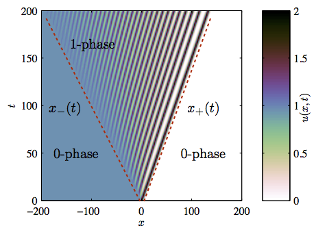
Figure 7: Contour plot of the KdV DSW solution found by GP [49] for $u_{-}=1$, $u_{+}=0$.

The 0-phase region, $S_{0}$, is the complement in the upper half plane, $S_{0}=(\overline{S_{1}})^{c}$, where the solution is described by $r$, the solution to the dispersionless Hopf equation (3.2). The boundary between $S_{0}$ and $S_{1}$,

$$\begin{split}\partial S&=\partial S_{-}\cup\partial S_{+},\\ \partial S_{\pm}&=\{(x,t)~{}|~{}x=x_{\pm}(t),~{}t>0\},\end{split}$$ (3.4)

is a free boundary and must be determined along with the solution in each region. It is this existence of a free boundary that make DSWs a challenge to analyze.

The step initial data (3.1) is used to initialize the Hopf equation (3.2) for the region $S_{0}$

$$r(x,0)=u_{\pm},\quad\pm x>0.$$

The Hopf equation then admits the piecewise, spatially uniform solution

$$r(x,t)=u_{\pm},\quad x\gtrless x_{\pm}(t),\quad t>0.$$

The GP matching conditions at the boundary $\partial S$ must determine both the location of the boundary as well as the values of the modulation variables there. One natural condition is achieved by equating the average $\overline{\varphi}$ of the modulated wave in $S_{1}$ to the dispersionless solution in $S_{0}$:

$$\begin{split}\overline{\varphi}|_{\partial S}=r|_{\partial S}~{}\Rightarrow~{}\overline{\varphi}(x_{\pm}(t),t)=u_{\pm}.\end{split}$$ (3.5)

Two additional conditions are achieved by continuous matching of $S_{0}$ to $S_{1}$. The rapidly varying periodic wave in $S_{1}$ can terminate in a slowly varying, in this case spatially uniform, region of $S_{0}$ in one of two ways, either the wave amplitude goes to zero (harmonic edge) or the wavenumber goes to zero (soliton edge). A choice must be made as to which boundary, $\partial S_{-}$ or $\partial S_{+}$, is associated with which edge. This choice is determined by an admissibility condition, the dispersive hydrodynamic analogue of an entropy condition. In order to identify the harmonic and soliton edges, GP appealed to the 2-wave curve (recall Sec. 2.1.2) of the Whitham modulation system.

Figure 8: KdV DSW modulation solution (solid) and mean $\overline{u}$ (dashed) for $t=175$, $u_{-}=1$, $u_{+}=0$.

As noted in Sec. 2.2.5, the harmonic edge limit occurs when $\mathbf{r}\to\mathbf{r}_{\mathrm{h}}=(r_{1},r_{1},r_{3})$ and the soliton edge limit occurs when $\mathbf{r}\to\mathbf{r}_{\mathrm{s}}=(r_{1},r_{3},r_{3})$. The 2-wave curve of eqs. (3.3) is parametrized according to

$$\begin{split}s&=V_{2}(r_{1},r_{2}(s),r_{3}),\quad s=\frac{x}{t},\quad r_{1}<r_{3},\end{split}$$ (3.6)

where $r_{1}$ and $r_{3}$ are constant. By the ordering $V_{2}(\mathbf{r}_{\mathrm{h}})<V_{2}(\mathbf{r}_{\mathrm{s}})$ (recall eqs. (2.89), (2.91) for the merged characteristic velocities in the soliton and harmonic limits respectively), we therefore observe the admissibility criterion

$$\begin{split}-r_{3}+2r_{1}<\frac{1}{3}(2r_{3}+r_{1})~{}\iff~{}r_{1}<r_{3}.\end{split}$$

Simply stated, the harmonic edge is on the left and the soliton edge is on the right. This determines the DSW’s orientation $d=1$ (recall Fig. 4). The DSW boundaries $x_{\pm}(t)$ are merged characteristics of the Whitham system

$$x_{-}(t) =s_{-}t,\qquad s_{-}=V_{2}(\mathbf{r}_{\mathrm{h}})$$ (3.7)

$$x_{+}(t) =s_{+}t,\qquad s_{+}=V_{2}(\mathbf{r}_{\mathrm{s}}),$$ (3.8)

straight lines in the $x$-$t$ plane.

With the DSW boundaries and its orientation determined, we can now identify the final two GP matching conditions

$$a_{-}=a|_{\partial S_{-}}=0,\quad k_{+}=k|_{\partial S_{+}}=0.$$ (3.9)

Utilizing the expressions in eqs. (2.56) and (2.58) for $\bar{\varphi}$ in the soliton and harmonic limit respectively, we can relate the matching conditions (3.5) and (3.9) to the following conditions on the Riemann invariants

$$r_{2}(s_{-})=r_{1}=u_{+},\quad r_{2}(s_{+})=r_{3}=u_{-}.$$ (3.10)

Now, using (2.53), (3.10) the modulation solution (3.6) can be explicitly written as

$$\frac{x}{t}=u_{+}+\frac{1}{3}\Delta\left(1+m-\frac{2m(1-m)\mathrm{K}(m)}{\mathrm{E}(m)-(1-m)\mathrm{K}(m)}\right),$$ (3.11)

where $\Delta=u_{-}-u_{+}$ is the initial jump height and $m=(r_{2}-u_{+})/\Delta$.

The macroscopic properties of the DSW include the motion of the harmonic and soliton edges (3.7), (3.8) with speeds found from (3.11) by computing the limits $m\to 0$ and $m\to 1$ respectively,

$$s_{-}=-\Delta+u_{+},\quad s_{+}=\frac{2}{3}\Delta+u_{+}.$$ (3.12)

The expansion speed of the DSW is $s_{+}-s_{-}=\tfrac{5}{3}\Delta$. Recalling the amplitude and wavenumber of the modulated wave (2.54), we can now determine the soliton edge amplitude $a_{+}$ and the harmonic edge wavenumber $k_{-}$

$$a_{+}=2\Delta,\quad k_{-}=\frac{1}{3}\sqrt{6\Delta}\,.$$ (3.13)

One can directly verify that the harmonic edge moves with the linear group velocity $s_{-}=\partial_{k}\omega_{0}(k_{-},u_{-})$ (recall eq. (2.58)). Similarly, the soliton edge moves according to the KdV soliton amplitude-speed relation $s_{+}=V_{\rm s}=u_{+}+a_{+}/3$ (recall eq. (2.56)). The soliton edge rises above $u_{+}$ so the polarity of this DSW is $p=1$ (recall Fig. 4).

So far, we have determined the macroscopic behavior of the DSW, its leading and trailing edge properties. The asymptotic behavior of the quantities of physical interest (the amplitude, the mean value and the wavenumber) in the vicinities of the trailing and leading edges is readily obtained by expanding expressions (2.54) along with the modulation solution (3.10), (3.11) for $m\ll 1$ and $1-m\ll 1$ respectively (see [49]). In particular, one has $a\simeq\tfrac{2}{3}(s-s_{-})$ near the trailing edge and $k\simeq\pi(2/3)^{1/2}/\ln({1}/(s_{+}-s))$ near the leading edge.

The internal DSW structure is recovered by inserting the 2-rarefaction modulation solution for $r_{1},r_{2},r_{3}$ given by eqs. (3.10), (3.11) into the traveling wave (2.55). An example is shown in Fig. 8 along with the weak limit $\overline{\varphi}$ where we used a zero phase shift.

A numerical comparison to the GP problem was undertaken in the work by Fornberg and Whitham [108], where they demonstrated excellent agreement between the numerics and the leading edge speed (3.12). The trailing edge exhibits decaying waves that propagate slower (more negative) than the trailing edge velocity (3.12). The structure of these waves has been studied by use of matched asymptotic expansions [109], where it was shown that they follow typical dispersive decay with amplitude proportional to $t^{-1/2}$. It is worth noting that there is a logarithmic correction to the motion of the soliton edge, leading Khruslov, who studied the GP problem using IST, to call the leading oscillation a quasi-soliton [110].

In summary, GP identified two matching conditions at each 1-phase, 0-phase boundary:

1. Matching the 1-phase wave mean to the 0-phase flow, eq. (3.5).

2. The zero amplitude and zero wavenumber reductions at the harmonic and soliton edges, respectively, eq. (3.9).

The location of the harmonic and soliton edges are determined by the existence of a self-similar, centered simple wave solution connecting them. These DSW “jump conditions” are the dispersive analogues of the Rankine-Hugoniot jump conditions of classical shock theory.

We have been considering the strictly negative or concave dispersion KdV equation (2.33). The dispersion sign is defined according to $\mathrm{sgn}\,[\partial_{kk}\omega_{0}(k,\overline{u})]$, $k>0$. The sign of dispersion provides an interpretation of the DSW orientation $d=1$. For concave dispersion, the group velocity decreases with increasing wavenumber so that the harmonic edge (larger wavenumber) must move slower than the soliton edge (zero wavenumber), hence the requisite orientation [111].

The transformation $x\to-x$, $u\to-u$ of the KdV equation (2.33) results in $u_{t}+uu_{x}-u_{xxx}=0$, exhibiting strictly positive or convex dispersion. The transformation causes the DSW to switch both its orientation and polarity to $d=-1$, $p=-1$.

3.1.2 Case $u_{-}<u_{+}$:

Implicit in the previous analysis of the GP problem is the existence of a modulated 1-phase region, which, due to wavebreaking of the dispersionless equation (3.2), is guaranteed when $u_{-}>u_{+}$. For the case $u_{-}<u_{+}$, a leading order description solely in terms of the dispersionless equation (3.2) is possible. This involves a centered rarefaction wave that takes the form

$$r(x,t)=\begin{cases}u_{-}&x<u_{-}t\\ \frac{x}{t}&u_{-}t\leq x<u_{+}t\\ u_{+}&u_{+}t<x\end{cases}.$$

Higher order corrections to this leading order solution have been investigated using matched asymptotic methods [112]. It was demonstrated that the left edge of the rarefaction wave exhibits small oscillations with typical dispersive long time amplitude decay $\mathcal{O}(t^{-1/2})$ and the right edge decays exponentially to $u_{+}$.

Combining the two cases $u_{-}\gtrless u_{+}$, we obtain the complete classification of the GP problem, represented in Fig. 9.

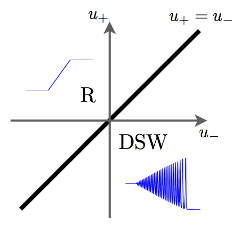
Figure 9: Classification of the GP problem including rarefaction waves (R) and DSWs.

3.1.3 DSW characteristics

Adopting tools from the theory of hyperbolic conservation laws, we consider the characteristic families associated with the KdV DSW in Fig. 10. External to the 1-phase region, the characteristics are straight lines $x=u_{\pm}t+x_{0}$. Internal to the DSW, there are three characteristic families of the Whitham equations given by

$$\Gamma_{i}=\left\{x(t)~{}\Big{|}~{}\frac{\,\mathrm{d}x}{\,\mathrm{d}t}=V_{i}\right\},\quad i=1,2,3.$$

The second characteristic family in Fig. 10c consists of the expansion fan solution in Fig. 10f. The first (slow) and third (fast) characteristic families in Figs. 10d,e are curved and emanate from the soliton, $x=s_{+}t$, and harmonic, $x=s_{-}t$, DSW boundaries, respectively. The slow and fast characteristics transfer information into the DSW. In long time, these characteristics become parallel to the opposite DSW boundaries $x=s_{-}t$ and $x=s_{+}t$, respectively. Thus, merger of the first and second characteristic families occurs at the trailing, harmonic edge of the DSW, coinciding with the group velocity of linear waves. The second and third characteristic families merge at the leading, soliton edge of the DSW, corresponding to propagation with the soliton phase velocity.

We also include the characteristic description of classical shocks Fig. 10a and rarefactions Fig. 10b for comparison.

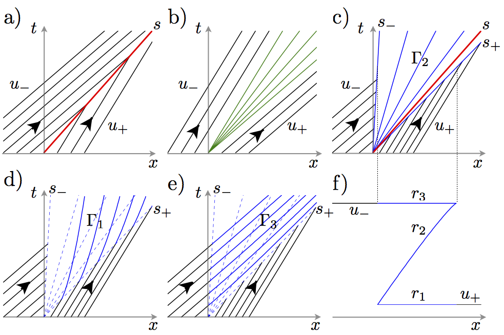
Figure 10: Characteristics for the classical shock (a), rarefaction (b) solutions of the Hopf equation (3.2) and the (c-e) KdV DSW solution along with the (f) Whitham modulation solution in Riemann invariants.

An equivalent but alternative approach to dispersive regularization of the Riemann problem can be achieved by choosing degenerate initial conditions for the 1-phase modulation equations that match the initial conditions (3.1) and yield a global solution. The degeneracy relates to the reduction in order of the Whitham equations when two Riemann invariants coincide. This procedure was first utilized in [113] and later applied to NLS [103], [114] and the KdV Riemann problem [4].

3.2 KdV: dispersive regularization of wavebreaking

The Riemann problem solution for the KdV equation provides a major insight into properties of DSWs. It is also of primary interest for applications since it utilizes the simplest, centered simple wave solutions of the associated modulation system. In many situations, however, this solution is not sufficient for the description of DSWs as the general scenario of simple wave evolution can involve a “spontaneous” formation of gradient catastrophe at some point $(x_{b},t_{b})$, whose location is determined by initial conditions [1]. To describe the dispersive regularization of wavebreaking, a more general solution of the Whitham equations is required.

We consider the KdV equation (2.33) with a “large and smooth” initial condition $u(x,0)=u_{0}(\varepsilon x)$ where $\varepsilon\ll 1$. It is convenient to rescale the independent variables in (2.33) by introducing $\tilde{x}=\varepsilon x$, $\tilde{t}=\varepsilon t$ (i.e. the new variables are the slow variables $X$ and $T$ from Sec. 2.2.2). Then, on dropping tildes, the initial value problem of interest is:

$$u_{t}+uu_{x}+\varepsilon^{2}u_{xxx}=0,\quad u(x,0)=u_{0}(x),$$ (3.14)

where $u_{0}(x)$ is a sufficiently smooth function with $u_{0}^{\prime}(x)<0$ on some interval $\Delta\subset\mathbb{R}$ with a single inflection point on $\Delta$.

Initially, if $\varepsilon$ is sufficiently small, one can neglect the dispersive term in (3.14) and approximate the solution $u=u(x,t;\varepsilon)$ of the small-dispersion KdV equation (3.14) by the solution $r(x,t)$ of the dispersionless KdV or Hopf equation (3.2) with the same initial condition $u_{0}(x)$. This is, actually, a rigorous result due to Lax and Levermore [50], stating that $\lim\limits_{\varepsilon\to 0}u(x,t;\varepsilon)=r(x,t)$ for $0<t<t_{b}$. The solution of the Hopf equation can be written in the implicit form

$$x-rt=W(r),$$ (3.15)

where $W(r)$ is the inverse function of $r=u_{0}(x)$ (see (2.18)).

Nonlinear evolution of $r(x,t)$ specified by the simple wave solution (3.15) leads to the steepening of the profile for $r(x)$ and eventually, to gradient catastrophe $|r_{x}|\to\infty$ at some point $(x_{b},t_{b},r_{b})$, found from the conditions $W^{\prime\prime}(r_{b})=0$, $t_{b}=-W^{\prime}(r_{b})$ and $x_{b}=r_{b}t_{b}+W(r_{b})$ (see, e.g., [1]).

Let the function $u_{0}(x)$ be analytic near the breaking point. Using symmetries of the KdV equation, which are also symmetries of the Hopf equation (3.2), one can always set the wave breaking point at $x_{b}=t_{b}=r_{b}=0$ so that, without loss of generality, we can assume that $W(0)=W^{\prime}(0)=W^{\prime\prime}(0)=0$. Expanding the solution (3.15) near this point assuming that $W^{\prime\prime\prime}(0)\neq 0$ and upon retaining the first nonvanishing term, we obtain the universal “cubic” behavior of the simple wave near the point of gradient catastrophe [49]:

$$x-rt=-\mu r^{3}\,,\quad\mu>0.$$ (3.16)

Using symmetries of the KdV equation, one can always set $\mu=1$. One can show that the curve $r(x,t)$ defined by (3.16) is single-valued for $t<0$ (pre-breaking), and triple-valued for $t>0$ (post-breaking). The latter behavior is unphysical and dispersion has to be taken into account for $t>0$ in order to regularize the singularity and prevent formation of the multivalued solution.

We now observe that the function $r(x,t)$ implicitly specified by equation (3.16) is the solution to the Cauchy problem for the Hopf equation (3.2) with the initial condition

$$r(x,0)=-x^{1/3},$$ (3.17)

where we assumed $\mu=1$ in (3.16). This establishes our interest in considering the KdV equation (3.14) with initial data in the form of an inverse cubic (3.17) as a universal model for the dispersive regularization of wavebreaking.

In what follows, we construct modulation solutions regularizing the wavebreaking for two types of initial data: (i) a monotone decreasing function with a single inflection point; (ii) a decaying, localized profile. The last case is of particular interest as it establishes a connection between Whitham theory and the semi-classical, Bohr-Sommerfeld approximation in quantum mechanics [115].

3.2.1 GP matching conditions

We now formulate free-boundary matching conditions for the modulation regularization of the general wavebreaking problem. These are essentially analogous to the GP conditions (3.5) for the Riemann problem but now, instead of matching the average $\overline{\varphi}$ to constant boundary values $u_{\pm}$ at the DSW edges, we require that $u_{\pm}=r(x_{\pm}(t),t)$, where $r(x,t)$ is the solution of the Hopf equation given by (3.15). Assuming the same DSW orientation $d=1$ established in the solution of the Riemann problem in Sec. 3.1, we identify the trailing $x_{-}(t)$ and leading $x_{+}(t)$ edges as harmonic ($m=0$) and soliton ($m=1$), respectively, and formulate general GP matching conditions for the KdV-Whitham system (3.3). We first note that it follows from (2.54) that in the harmonic and soliton limits, the mean of the cnoidal wave solution $\overline{\varphi}$ becomes

$$\begin{split}m=0:\quad\overline{\varphi}=r_{3},\\ m=1:\quad\overline{\varphi}=r_{1}.\end{split}$$ (3.18)

The generalized GP matching conditions are then formulated as

$$\begin{array}[]{l}x=x_{-}(t):\qquad r_{2}=r_{1}\,,\ \ r_{3}=r\,,\\ x=x_{+}(t):\qquad r_{2}=r_{3}\,,\ \ r_{1}=r\,,\end{array}$$ (3.19)

where $r(x,t)$ is given by (3.15). The DSW boundary $\partial S$ (3.4) is defined by the merged characteristics of the Whitham system for $m=0$, where $x=x_{-}(t)$, and $m=1$, where $x=x_{+}(t)$ (see (2.89), (2.91)). Then $x_{\pm}(t)$ are found from the ordinary differential equations

$$\frac{dx_{-}}{dt}=-r_{-}+2r_{12}\,,\ \ \frac{dx_{+}}{dt}=\frac{1}{3}(2r_{23}+r_{+}),$$ (3.20)

where $r_{-}(t)\equiv r(x_{-}(t),t)$ and $r_{12}(t)\equiv r_{1}(x_{-}(t),t)=r_{2}(x_{-}(t),t)$ is the value of the merged Riemann invariant at $x=x_{-}(t)$. Analogously $r_{+}(t)\equiv r(x_{+}(t),t)$ and $r_{23}(t)\equiv r_{2}(x_{+}(t),t)=r_{3}(x_{+}(t),t)$. Note that, unlike in the solution of the Riemann problem, where the DSW edges are defined by regular characteristics of the Whitham modulation system, the general matching regularization (3.19) implies that the DSW edges $x_{\pm}(t)$ specified by (3.20) are characteristic envelopes, i.e., singular solutions of the general characteristic ODEs defined on the solution of the GP problem. As a result, the corresponding merged Riemann invariants $r_{12}$ and $r_{23}$ are allowed to vary along the edge curves [49].

One can show using (2.57) – (2.59) that the edge definitions (3.20) can be re-written in a physically transparent form

$$\frac{dx_{-}}{dt}=c_{\rm g}(k_{-},\overline{\varphi}_{-});\qquad\frac{dx_{+}}{dt}=V_{\rm s}(a_{+},\overline{\varphi}_{+}),$$ (3.21)

where $c_{\rm g}(k,\overline{\varphi})=\partial_{k}\omega_{0}(k,\overline{\varphi})$ is the linear group velocity and $V_{\rm s}(a_{s},\overline{\varphi})$ is the speed of the KdV soliton of amplitude $a_{\rm s}$ riding on the backround $\overline{\varphi}$. It follows from (3.18), (3.19) that at the edges $\overline{\varphi}_{\pm}=r_{\pm}$. Also $a_{+}=a_{\rm s}(x_{+},t)$, $k_{-}=k(x_{-},t)$.

The definitions (3.21) of the trailing and leading edges have a natural interpretation as DSW kinematic boundary conditions while the matching conditions (3.19) are dynamic boundary conditions, using standard terminology from water wave theory [1]. We also note that the edge definitions in the form (3.21) admit a natural extension to DSW theory in non-integrable dispersive hydrodynamics, for which modulation systems do not possess Riemann invariant structure.

3.2.2 Hodograph solution: the scalar potential

The generalized GP problem (3.3), (3.19) is a nonlinear free-boundary problem, which is generally very difficult to solve directly. However, it admits a remarkable simplification when reformulated in hodograph space with Riemann invariants $r_{1},r_{2},r_{3}$ as independent variables. First of all, one can notice that the DSW edges $x_{\pm}(t)$ in the $x$-$t$ plane map to planes in hodograph space. These are given by $r_{1}=r_{2}$ (the trailing edge) and $r_{2}=r_{3}$ (the leading edge). Then, using that $V_{3}(r_{1},r_{1},r_{3})=r_{3}$ and $V_{1}(r_{1},r_{3},r_{3})=r_{1}$ (see Sec. 2.2.5) and comparing the generalized hodograph solution (2.24) with the simple-wave solution (3.15) at the above boundaries, we obtain the boundary conditions for the linear Tsarev system (2.25) [73, 106]

$$\begin{split}W_{3}(r_{1},r_{1},r_{3})=W(r_{3}),\\ W_{1}(r_{1},r_{3},r_{3})=W(r_{1})\,.\end{split}$$ (3.22)

Further, one can show that $\partial_{1}W_{3}(r_{1},r_{1},r_{3})=\partial_{3}W_{1}(r_{1},r_{3},r_{3})=0$ [106] and, since $r=r_{3}$ along $x=x_{-}(t)$ and $r=r_{1}$ along $x=x_{+}(t)$, the conditions (3.22) can be replaced by

$$\begin{split}W_{3}(0,0,r_{-})=W(r_{-});\\ W_{1}(r_{+},0,0)=W(r_{+})\,.\end{split}$$ (3.23)

Note that the boundary conditions (3.23) are linear and specified on known boundaries: the characteristics of the Tsarev system (2.25). Thus the problem (2.25), (3.23) is a linear Goursat (Darboux) problem [116]. This remarkable full linearization of the nonlinear free-boundary, generalized GP problem in hodograph space is in sharp contrast with the well known poor compatibility of initial-value problems with the classical hodograph transform [1].

We now use the Goursat data (3.23) for $W_{j}$ to formulate the counterpart boundary conditions for the EPD system (2.98) defining the $q$-function, a scalar potential for the solutions $W_{j}$ to the Tsarev equations (2.25). The boundary conditions for $q(r_{1},r_{2},r_{3})$ are obtained by substituting (3.23) in the transformation (2.97) and then integrating the resulting ODEs. As a result we obtain

$$q(r,0,0)=q(0,0,r)=\frac{1}{2}r^{-1/2}\int^{r}_{0}y^{-1/2}W(y)\,\mathrm{d}y\,.$$ (3.24)

We note that $r_{2}=r_{3}=r_{23}$ and $r_{2}=r_{1}=r_{12}$ corresponding to the DSW leading and trailing edges, respectively, are singular surfaces for the EPD system (2.98). For the elliptic parameter $m=(r_{2}-r_{1})/(r_{3}-r_{1})$ in the DSW to be defined in the entire interval $0\leq m\leq 1$ for all $t$, one must impose additional conditions of non-singularity of $q$ at these surfaces,

$$q(r_{+},r_{23},r_{23})<\infty,\quad q(r_{12},r_{12},r_{-})<\infty\,.$$ (3.25)

If one of the Riemann invariants is constant, the function $g$ becomes a function of two variables and only one of the conditions (3.24) should be used. This is the case, e.g., if one considers the GP problem with initial function $u_{0}(x)$, which monotonically decreases for $x<0$ and is a constant for $x>0$, leading to DSW propagation into a uniform “gas”, a constant equilibrium state. For smooth, monotonically decreasing initial conditions $u_{0}(x)$, causing all three Riemann invariants in the modulation solution to be non-constant, an alternative form of the boundary condition for the EPD system can be used [96]: $q(r,r,r)=W(r)$.

Using the boundary conditions (3.24), we can identify the functions $\Phi_{j}(\lambda)$ in the general solution (2.104) of the EPD equation. These are shown in [106] to be expressed in terms of the Abel transform of the inverse function $W(r)$. Finally, the solution for the function $q({\bf r})$ can be represented in compact form [106]

$$\begin{split}q=\frac{1}{\pi(r_{3}-r_{2})^{1/2}}\int\limits^{r_{3}}_{r_{2}}\frac{W(\tau)}{\sqrt{\tau-r_{1}}}K(z)\,\mathrm{d}\tau\\ +\frac{1}{\pi(r_{2}-r_{1})^{1/2}}\int\limits^{r_{2}}_{r_{1}}\frac{W(\tau)}{\sqrt{r_{3}-\tau}}K\left(z^{-1}\right)\,\mathrm{d}\tau\,,\end{split}$$ (3.26)

where $K(z)$ is the complete elliptic integral of the first kind and

$$z=\left[\frac{(r_{2}-r_{1})(r_{3}-\tau)}{(r_{3}-r_{2})(\tau-r_{1})}\right]^{1/2}.$$ (3.27)

A different, double integral form of the solution $q({\bf r})$ was obtained in [96], where also the invertibility of the hodograph solution (2.99) for $r_{j}(x,t)$ was proved.

3.2.3 Regularization of cubic wave breaking

As was shown in Sec. 3.2, the regularization of “cubic” wavebreaking is of particular interest, so we shall construct the corresponding modulation solution explicitly. A general way to approach this problem would be to substitute the inverse function $W(r)=-r^{3}$ of the initial condition (3.17) into the solution (3.26) for the $q$-function and then generate the modulation solution $\{r_{j}\}_{j=1}^{3}$ in an implicit hodograph form (2.99). Instead, we notice that the dispersionless limit solution (3.15) has scaling properties, namely $r=t^{1/2}R(x/t^{3/2})$, where $R(\zeta)$ satisfies the algebraic equation $R^{3}-R+\zeta=0$. Then one can directly construct the modulation solution having the same scaling properties and require that the two solutions continuously match according to the GP conditions (3.19) at the phase transition boundaries $x_{\pm}(t)$, the DSW edges. The family of modulation solutions having the necessary scaling properties was shown in Sec. 2.2.6 to be generated by homogeneous solutions of the EPD system. To this end, we identify the scaling parameter $\gamma=1/2$ in (2.103) and find the corresponding homegeneity degree $\alpha=1+1/\gamma=3$. Thus the necessary homogeneous solution is $q_{3}=5s_{1}^{3}-12s_{1}s_{2}+8s_{3}$, where $s_{j}({\bf r})$ are the elementary symmetric polynomials (see (2.102) and (2.70)). We now set $q=Cq_{3}$, where $C$ is a constant to be found from the matching conditions (3.19), or their equivalent $q(r,r,r)=W(r)=-r^{3}$ [96] for strictly monotone initial functions. We find that $C=-1/35$. As a result, the generalized similarity modulation solution has the form

$$r_{j}(x,t)=t^{1/2}R_{j}(\zeta),\ \ \zeta=x/t^{3/2},$$ (3.28)

where $R_{j}$, $j=1,2,3$ are found from the system

$$\begin{split}\zeta-V_{i}(R_{1},R_{2},R_{3})=-\tfrac{1}{35}\left(1-\frac{L}{\partial_{i}L}\partial_{i}\right)q_{3},\\ i=1,2,3,\end{split}$$ (3.29)

with $L\equiv L({\bf R})$, $q_{3}\equiv q_{3}({\bf R})$, and $\partial_{i}\equiv\partial_{R_{i}}$.

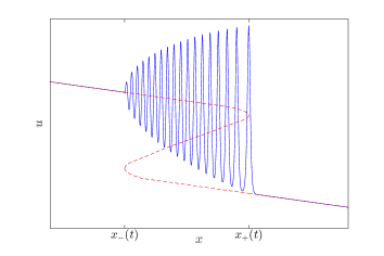
Figure 11: Sketch of the dispersive regularization of cubic wavebreaking in the KdV equation (solid) along with the modulation solution $r_{3}(x,t)\geqslant r_{2}(x,t)\geqslant r_{1}(x,t)$ (dashed).

The constructed similarity solution describes the evolution of the triple-valued function [60] $\{r_{1}(x,t),r_{2}(x,t),r_{3}(x,t)\}$ (see Fig. 11), defined for all $t>0$ within the expanding interval $[x_{-},x_{+}]$, where

$$x_{-}(t)=-2\sqrt{3}t^{3/2},\quad x_{+}(t)=\frac{\sqrt{15}}{27}t^{3/2}\,.$$ (3.30)

The latter expressions are obtained by integrating (3.20). We stress that the obtained modulation solution does not coincide with the formal triple-valued solution (3.16) of the Hopf equation for $t>0$. Substituting $r_{1}(x,t)$, $r_{2}(x,t)$, $r_{3}(x,t)$ specified by (3.28), (3.29) into the “carrier” traveling wave solution (2.55), one obtains the full asymptotic description of the DSW. The phase of the traveling solution is $\theta=k(x-Vt-\xi_{0})$ with the modulation phase correction $\xi_{0}(x,t)=q({\bf r})=-\tfrac{1}{35}q_{3}({\bf r})$ (see Sec. 2.2.6). A schematic of dispersive regularization of cubic wavebreaking is shown in Fig. 11.

The amplitude of the lead soliton is found from the leading edge definition in eq. (3.21), yielding $\dot{x}_{+}=\overline{\varphi}_{+}+a_{+}/3$ (see (2.56)), whereas the soliton background satisfies $\overline{\varphi}_{+}=r_{+}=t^{1/2}R_{+}$, $R_{+}\approx-1.065$ being the smallest root of the equation $R^{3}-R+\sqrt{15}/27=0$. As a result, using (3.30) we obtain

$$a_{+}(t)=At^{1/2},\quad A=\tfrac{\sqrt{15}}{6}-3R_{+}\approx 3.840$$ (3.31)

The trailing edge wavenumber $k_{-}$ is found from the trailing edge definition in eq. (3.21) yielding $\dot{x}_{-}=\overline{\varphi}_{-}-3k_{-}^{2}$ where the vanishing amplitude wave background satisfies $\overline{\varphi}_{-}=r_{-}=t^{1/2}R_{-}$, $R_{-}=\sqrt{3}$ being the greatest root of $R^{3}-R-2\sqrt{3}=0$. As a result,

$$k_{-}(t)=(3t)^{1/4}.$$

Concluding, we note that the modulation solution for the cubic GP problem was first studied numerically in the original GP paper [49], where one can also find the asymptotic behavior of the Riemann invariants near the trailing and leading edges. One qualitative difference to the GP solution for the Riemann step problem is that in the step regularizing DSW, the wave amplitude grows linearly near the trailing edge, $a\sim(x-x_{-})$, which results in a “Martini glass” DSW envelope shape, while in the case of cubic wavebreaking, one has $a\sim\sqrt{x-x_{-}}$, a “Bordeaux glass” shape (cf. Fig. 8 and Fig. 11). The latter asymptotic behavior is, in fact, generic for the dispersive wavebreaking regularization. Another difference is that the lead amplitude $a_{+}$ as well as the trailing edge wavenumber $k_{-}$ grow as $t^{1/2}$ and $t^{1/4}$ respectively, in the KdV cubic wavebreaking problem while they remain constant in the Riemann problem.

The modulation solution (3.29) was first obtained by Potëmin [117] by analyzing the relevant Krichever algebro-geometric solution [85]. This solution was also obtained in [118] within the framework of the IST based semi-classical Lax-Levermore approach [50]. Stability of the modulation solution regularizing cubic wave breaking was investigated numerically in [119].

3.2.4 Evolution of decaying profiles

We now consider KdV evolution (3.14) of decaying initial profiles $u_{0}(x)$: $u_{0}(x)\to 0$ as $|x|\to\infty$. Since such an evoution, under some mild restricions imposed on the decay rate of $u_{0}(x)$, can be described using the IST, it will be particularly instructive to see how the IST results compare with the results of the modulation approach employed here. We shall separately consider the elevation and depression cases and then combine them into a dispersive counterpart of the classical problem of $N$-wave evolution modeled by the solution of Burger’s equation [1].

Localized elevation

With a mild violation of generality, we assume that the initial hump $u_{0}(x)=u_{0}^{+}(x)\geq 0$, has semi-infinite support so that $u_{0}^{+}(x)\equiv 0$ for $x>0$ and $u_{0}^{+}(x)>0$ for $x<0$. This corresponds to the aforementioned propagation of a DSW into a uniform “gas”. We also assume that $u_{0}(x)$ has a single maximum at some $x=x^{*}<0$: $u_{0}^{+}(x^{*})=h>0$, $(u_{0}^{+})^{\prime}(x^{*})=0$ and $u_{0}^{+}(x)\to 0$ as $x\to-\infty$. Now one can assume, without a further abuse of generality, that the wavebreaking point is at $x=0,t=0$. A typical form of the initial profile is shown in Fig. 12a.

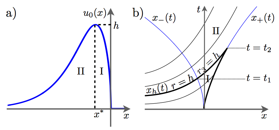
Figure 12: a) initial localized elevation $u_{0}(x)$; b) characteristics of the modulation system for the localized elevation problem.

Since $u_{0}^{+}(x)=0$ for $x\geq 0$, the GP matching condition at the leading edge (3.19) is $r_{1}(x_{+},t)=0$ which, together with the modulation equation for $r_{1}$, implies that $r_{1}=0$ throughout the modulation solution and there are only two varying Riemann invariants: $r_{2}$ and $r_{3}$. To handle non-monotonicity of the initial function $u_{0}^{+}(x)$, we introduce a “two-sheeted” hodograph transform [120, 106] so that we have the hodograph surface consisting of two copies of the hodograph plane $(0,r_{2},r_{3})$ which are glued together along the line $r_{3}=h$. The construction is analogous to the Riemann surface covering of the complex plane. On each sheet of the hodograph surface, we define the mapping (2.99) $(r_{2},r_{3})\leftrightarrow(x,t)$ – bijectivity of this mapping is not automatic and must later be proven for the particular solution – reducing the modulation system (2.51) for $r_{2}$ and $r_{3}$ to a single EPD equation (2.98) for the function $q_{k}(r_{2},r_{3})$ with $k=I,II$ labeling the sheets of the hodograph surface. Each function $g_{I,II}$ is defined inside the triangle $0\leq r_{2}\leq r_{3}\leq h$ of the respective sheet. We now introduce two monotone functions $W_{I}(r)$ and $W_{II}(r)$ so that $W_{I}(r)$, $r\in[0,h]$, is the inverse of the decreasing part of the initial profile $u_{0}^{+}(x)$ and $W_{II}(r)$, $r\in(0,h]$, is the inverse of the increasing part with $W_{I}(x^{*})=W_{II}(x^{*})=h$. Then the boundary conditions for the functions $q_{I}(r_{2},r_{3})$ and $q_{II}(r_{2},r_{3})$ assume the form

$$\begin{split}q_{I,II}(0,r_{3})=\frac{1}{2}r_{3}^{-1/2}\int\limits^{r_{3}}_{0}y^{-1/2}W_{I,II}(y)\,\mathrm{d}y,\\ q_{I}(r_{2},h)=g_{II}(r_{2},h).\end{split}$$

One must also add the non-singularity conditions (3.25) for $q_{I}(r,r)$, but not for $q_{II}$, which is defined uniquely by continuous matching with $q_{I}$.

The conditions at $r_{2}=0$ follow from the GP matching (3.19) at the trailing edge and are analogous to (3.24) while the condition at $r_{3}=h$ is new and provides a continuous matching of the hodograph solutions defined on the sheets $I$ and $II$ along the characteristic $r_{3}=h$ which is common for both sheets.

The resulting solution of the EPD equation can be compactly represented in the form [106]:

$$\begin{split}q_{I}(r_{2},r_{3})=\int^{r_{2}}_{0}\kappa(r,r_{2},r_{3})W_{I}(r)\,\mathrm{d}r\\ +\int^{r_{3}}_{r_{2}}\kappa(r_{2},r,r_{3})W_{I}(r)\,\mathrm{d}r,\end{split}$$ (3.32)

$$q_{II}(r_{2},r_{3})=g_{I}+\int^{h}_{r_{3}}\kappa(r_{2},r_{3},r)D(r)\,\mathrm{d}r,$$ (3.33)

where $D(r)=W_{I}(r)-W_{II}(r)$ and

$$\kappa(x,y,z)=\frac{1}{\pi\sqrt{(z-x)y}}\ \mathrm{K}\left(\frac{z-y}{z-x}\frac{x}{y}\right).$$

Note that the solution (3.32) on the first sheet is equivalent to $q(0,r_{2},r_{3})$ given by (3.26) with $W(r)\equiv W_{I}(r)$. One can readily show that $\partial_{3}q_{I}(r_{2},h)=\partial_{3}q_{II}(r_{2},h)$ thus ensuring the continuity of the modulation solution (2.99) across the characteristic $r_{3}=h$.

The analysis of the mapping $(r_{2},r_{3})\mapsto(x,t)$ specified by (2.99) with $r_{1}\equiv 0$, $q=q_{I,II}$ shows that it maps the triangle $0\leq r_{2}\leq r_{3}$ of the sheet $I$ to some finite region of the $x,t$ plane, bounded by the edge curves $x_{-}(t),x_{+}(t)$ defined by (3.20), and the characteristic $x_{h}(t)$ transferring the Riemann invariant $r_{3}=h$ (see Fig. 12b). Within the interval $t\in[0,t_{1}]$, where $t_{1}$ is found from the condition $r_{3}(x_{-}(t_{1}),t_{1})=h$, the modulation solution is fully specified by $q_{I}$ and describes a DSW regularizing wavebreaking of the monotonically decreasing part of the initial function $u_{0}(x)$. For $t\in[t_{1},t_{2}]$, where $t_{2}$ is found from the condition $r_{3}(x_{+}(t_{2}),t_{2})=h$, the solution $(r_{2}(x,t),r_{3}(x,t))$ consists of two parts generated by $q_{I}$ and $q_{II}$ respectively, each part being defined within its own domain in the ($x,t$) plane. The domains have common boundary defined by the characteristic transferring the maximum value $r_{3}=h$. Finally, for $t>t_{2}$, the modulation solution is fully defined by the function $q_{II}$, which maps the triangle $0\leq r_{2}\leq r_{3}$ on the second sheet of the hodograph surface onto the infinite region in the $x,t$-plane bounded by the characteristics $[x_{-}(t),x_{+}(t)]$, $t>t_{2}$ with the leading edge characteristic being a straight line $x=\tfrac{2}{3}r_{3}t$. The modulation solution generated by $g_{II}$ describes the interaction of the DSW with the rarefaction wave developing due to the evolution of the increasing part of the initial profile $u_{0}(x)$. This intepretation becomes particularly lucid when the initial profile has the shape of a rectangular barrier [121].

Strictly speaking, one should now show that the obtained solution is global, i.e., the mapping $(r_{2},r_{3})\mapsto(x,t)$ is invertible for all $t$. Partial proof of this invertibility can be found in [122]. Here, instead of giving a full mathematical proof, we shall show that the obtained modulation solution implies a long-time asymptotic behavior for $r_{j}(x,t)$ consistent with the predictions of IST analysis for the case of a localized profile. This agreement is a strong indication that the obtained modulation solution is valid for all $t$.

The analysis of the mapping $(r_{2},r_{3})\mapsto(x,t)$ specified by (2.99) with $r_{1}\equiv 0$, $q=q_{I,II}$ shows that it maps the triangle $0\leq r_{2}\leq r_{3}$ of the sheet $I$ to some finite region of the $x,t$ plane, bounded by the edge curves $x_{-}(t),x_{+}(t)$ defined by (3.20), and the characteristic $x_{h}(t)$ transferring the Riemann invariant $r_{3}=h$ (see Fig. 12 b)). Within the interval $t\in[0,t_{1}]$, where $t_{1}$ is found from the condition $r_{3}(x_{-}(t_{1}),t_{1})=h$, the modulation solution is fully specified by $q_{I}$ and describes a DSW regularizing the wavebreaking of the monotonically decreasing part of the initial function $u_{0}(x)$. For $t\in[t_{1},t_{2}]$, where $t_{2}$ is found from the condition $r_{3}(x_{+}(t_{2}),t_{2})=h$, the solution $(r_{2}(x,t),r_{3}(x,t))$ consists of two parts generated by $q_{I}$ and $q_{II}$ respectively, each part being defined within its own domain in the ($x,t$) -plane. The domains have common boundary defined by the characteristic transferring the maximum value $r_{3}=h$. Finally, for $t>t_{2}$ the modulation solution is fully defined by the function $q_{II}$ which maps the triangle $0\leq r_{2}\leq r_{3}$ on the second sheet of the hodograph surface onto the infinite region in the $x,t$-plane bounded by the characteristics $[x_{-}(t),x_{+}(t)]$, $t>t_{2}$ with the leading edge characteristic being a straight line $x=\tfrac{2}{3}r_{3}t$. The modulation solution generated by $q_{II}$ describes the interaction of the DSW with the rarefaction wave developing due to the evolution the increasing part of the initial profile $u_{0}(x)$. This interpretation becomes particularly lucid when the initial profile has the shape of a rectangular barrier [121].

Strictly speaking, one should now show that the obtained solution is global, i.e. the mapping $(r_{2},r_{3})\mapsto(x,t)$ is invertible for all $t$. Partial proof of this invertibility can be found in [122]. Here, instead of giving a full mathematical proof, we shall show that the obtained modulation solution implies a long-time asymptotic behavior for $r_{j}(x,t)$ consistent with the predictions of the IST analysis applicable in the case of localized profile. This agreement is a strong indication that the obtained modulation solution is valid for all $t$.

The asymptotic behavior of the modulation solution can be conveniently studied by representing the hodograph formulae (2.21) in the form

$$t=\frac{W_{3}-W_{2}}{V_{3}-V_{2}};\quad x=V_{3}(r_{2},r_{3})t+W_{3}(r_{2},r_{3})\,.$$ (3.34)

The asymptotic behavior of $m=r_{2}/r_{3}$ for $t\gg 1$, following from (3.34), is then found as [106]

$$m\simeq 1-e^{-t/T(r_{3})},$$ (3.35)

where

$$T(r_{3})=-\frac{3}{4\pi}r_{3}^{-1/2}\int\limits^{h}_{r_{3}}\frac{D^{\prime}(r)}{\sqrt{r-r_{3}}}\,\mathrm{d}\tau\,.$$ (3.36)

Since $D^{\prime}(r)<0$, one has $T(r_{3})>0$, implying $m\to 1$ as $t\to\infty$ at any fixed point of the $x$-domain of $r_{3}$. This has a clear interpretation as the asymptotic transformation of a localized elevation into a solitary wavetrain, which is consistent with IST predictions.

For $x$ in (3.34) we obtain

$$t\gg 1:\quad x=\frac{2}{3}r_{3}t+x_{0}(r_{3})+o(1),$$ (3.37)

where

$$\begin{split}x_{0}(r_{3})=\frac{1}{2\pi(r_{3})^{1/2}}\int\limits^{h}_{r_{3}}\ln\left(\frac{r-r_{3}}{r}\right)\frac{D^{\prime}(r)}{\sqrt{r_{3}-r}}\,\mathrm{d}r\\ +\frac{1}{2(r_{3})^{1/2}}\int\limits^{r_{3}}_{r_{0}}\frac{W_{I}(r)}{\sqrt{r_{3}-r}}\,\mathrm{d}r\,.\end{split}$$

Invoking the traveling wave amplitude $a=2(r_{2}-r_{1})=2r_{2}$, and using the asymptotics (3.35), implying $r_{2}\to r_{3}$ as $t\to\infty$, we identify the leading order behavior in (3.37) with the universal “triangular” asymptotic distribution of the amplitude $a=3{x}/{t}$ in a solitary wavetrain consisting of non-interacting solitons [1]. The amplitude of the lead soliton in the train $a_{\max}=2h$ is determined by the maximum value $(r_{3})_{\max}=h$, and is the same as for the lead soliton in a DSW resulting from the Riemann problem with an initial step of magnitude $h$, see Sec. 3.1. Thus, the range of amplitudes in the train is $0<a<2h$, and the spatial extent of the train is $0<x<\tfrac{2}{3}ht$. The correction $x_{0}(r_{3})$ in (3.37) is due to weak soliton interactions in the train evolving from the initial localized elevation of the particular form $u_{0}(x)$.

The asymptotic solitary wavetrain is also characterized by a wavenumber $k$, which can be interpreted as the soliton density distribution. From (2.54), (3.35), (3.36), (3.37) we obtain, with account of the normalization of $x$ and $t$ in (3.14), the long-time asymptotic behavior

$$k\simeq\frac{1}{t}F(a),$$ (3.38)

where

$$F(a)=-\frac{1}{\varepsilon}\frac{\sqrt{6}}{4}\int\limits^{h}_{a/2}\frac{D^{\prime}(r)}{\sqrt{r-a/2}}\,\mathrm{d}r.$$ (3.39)

From the balance relation $kdx=f(a)da$, where $\tfrac{1}{2\pi}f(a)$ is the distribution function of solitons over amplitude [1], we find, on using $a=3x/t$ and comparing with (3.38), that $3f(a)=F(a)$.

Each soliton corresponds to a discrete eigenvalue $\lambda_{n}=-\eta_{n}^{2}$ of the quantum-mechanical Schrödinger operator with the potential $-u_{0}(x)/6$, which is the Lax operator associated with the KdV equation (3.14). By making the substitution $r=u_{0}(x)$, $a=2\eta^{2}$ in (3.39), we obtain the Weyl formula for the semi-classical density of the (transformed) eigenvalues $\eta_{n}$ on the interval $[0,\sqrt{h}]$ (see, e.g., [123])

$$\varphi(\eta)\sim\frac{1}{\pi\varepsilon}\oint\frac{\eta}{\sqrt{u_{0}(x)-\eta^{2}}}\,\mathrm{d}x.$$ (3.40)

In quantum mechanics the distribution (3.40) is a direct consequence of the famous Bohr-Sommerfeld semi-classical quantization rule [115, 1]. In the framework of soliton theory, it was first used by Karpman [124] (see also [66]).

The total number of solitons “contained” in the initial elevation $u_{0}(x)$ and released as $t\to\infty$ can be estimated by evaluating the integral

$$N\simeq\frac{1}{2\pi}\int\limits^{\infty}_{-\infty}k\,\mathrm{d}x=\frac{1}{6\pi}\int\limits^{2h}_{0}F(a)\,\mathrm{d}a.$$ (3.41)

Substituting (3.39) into (3.41) we obtain, upon reversing the order of integration,

$$N\sim\frac{1}{\pi\epsilon}\int\limits^{\infty}_{-\infty}[u_{0}(x)]^{1/2}\,\mathrm{d}x,$$ (3.42)

which is the standard quantum-mechanical result for the total numer of discrete eigenvalues in the semi-classical approximation and hence, the total number of solitons found via the IST [1].

Thus, remarkably, modulation theory gives the correct analytical description of the long-time asymptotic solitary wavetrain, even though formally the underlying modulation description is based on the asymptotic equivalence of spatial averaging over a large number of oscillations to averaging over one period [48, 1], which is not applicable here as the period of the traveling wave tends to infinity in the soliton limit. We note that the direct description of the solitary wavetrain as an esnsemble of non-interacting solitons readily yields the formula (3.38) [1] but does not provide information about the distribution function $F(a)$, which is related to the KdV initial condition. In conclusion, we note that the modulation description of the evolution of a localized initial elevation without the restriction $u_{0}(x>0)\equiv 0$ imposed here on the initial data was obtaibed in [125] and leads to the same asymptotic formulae (3.37), (3.38).

Localized depression

We now consider the KdV evolution of a localized depression $u_{0}(x)=u_{0}^{-}(x)\leq 0$, where we assume $u_{0}^{-}(x)=-u_{0}^{+}(-x)$, the function $u_{0}^{+}(x)$ being the localized elevation described above. This problem was studied in the modulation theory framework in [106, 126]. Similar to the already considered elevation case, wavebreaking of a localized depression with initial form $u_{0}^{-}(x)$ occurs at the boundary with a uniform state implying now $r_{3}=0$ and $-h\leq r_{1}\leq r_{2}\leq 0$. Wavebreaking is regularized by the generation of a DSW, and the corresponding modulation solution for the function $q(r_{1},r_{2})$ is constructed in a completely analogous way to the one for the elevation case. In fact, it can be obtained from solution (3.32), (3.33) by replacing $r_{2}\to-r_{2}$, $r_{3}\to-r_{1}$, $D(r)\to-D(r)$. Remarkably, the “depression” DSW exhibits solitons near its leading edge, while globally, there is no discrete spectrum in the associated scattering problem. At the level of modulation theory, this is a direct consequence of hyperbolicity of the modulation equations so that the DSW solution is confined to the finite region $(x_{-}(t),x_{+}(t))$ and is not affected, for $t=O(1)$, by the behavior of the “external” solution at $|x|\to\infty$. The intermediate solitonic asymptotics in the “solitonless” KdV evolution were studied in [127] using the IST.

While the intermediate asymptotic behaviors of initial elevation and depression evolution reveal a great deal of similarity, the respective long-time asymptotic solutions are drastically different. As was shown in [128], the long-time asymptotic of the modulation solution for the initial depression is given by:

$$t\gg 1:\quad x=2r_{1}t-\frac{1}{2}at+o(t^{1/2}),$$ (3.43)

$$a(x,t)=2(r_{2}-r_{1})\simeq\frac{4}{t^{1/2}}\left(\tau\right)^{1/4}A^{1/2}\left(-\tau\right).$$ (3.44)

Here

$$\tau=-{x}/{2t},\quad A(y)=\frac{2}{\pi}\int\limits^{x_{2}}_{x_{1}}[y-u_{0}^{-}(x)]^{1/2}\,\mathrm{d}x,$$

where $x_{1}(y)<x_{2}(y)$ are the roots of the equation $u_{0}^{-}(x)=y$. Equation (3.44) describes the asymptotic behavior of the modulated wave’s amplitude $a$. One can see that $a\to 0$ as $t\to\infty$. Since $m=-a/2r_{1}$, formula (3.44) also implies $m\to 0$ as $t\to\infty$, i.e., nonlinear modulation theory prescribes the asymptotic transformation of the initial depression into a modulated linear wave packet in full agreement with results from IST [129]. We note that the function $A(y)$ is related to the logarithm of the transmission coefficient for the potential barrier $-u_{0}^{-}(x)$. The behavior $a\sim t^{-1/2}$ prescribed by (3.44) is consistent with linear wavepacket energy conservation and can be obtained as an exact solution of the modulation equations for linear dispersive waves [1]. Linear modulation theory, however, does not provide a coefficient of $t^{-1/2}$ in (3.44), which is related to the KdV initial conditions.

The wave number distribution in the wave packet is found to be

$$\varepsilon^{2}k^{2}=-\frac{x}{3t}-\frac{1}{6}a(x,t)+O(1/t),\quad x<0\,.$$ (3.45)

The first term in the expansion (3.45) corresponds to the motion of the linear wave packet to the left with the group velocity $\omega^{\prime}(k)=-3\varepsilon k^{2}=x/t$, again in full agreement with linear modulation theory.

We note that the evolution of an initial depression on shallow water leading to the generation of a DSW has been observed in water tank experiments [22, 27] that showed very good agreement with the KdV predicted dynamics. Note that in [27], an unconventional “T-KdV” version of the KdV equation was used where the roles of time and space were swapped.

Dispersive evolution of $N$-wave

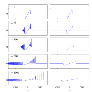
Figure 13: $N$-wave evolution in dispersive (KdV, left) and dissipative (Burger’s, right) hydrodynamics.

Finally, we consider the KdV evolution of an $N$-wave. The $N$ wave represents the universal waveform occuring in the asymptotic evolution of bipolar profiles in viscous fluid dynamics, described, e.g., by Burger’s equation [1]. Such density profiles leading to $N$ waves naturally occur in supersonic flows around finite-length objects, e.g., an airfoil. The classical $N$-wave represents a combination of two viscous shocks of opposite polarity propagating in opposite directions into the same equilibrium state, and connected by a rarefaction wave (see the initial state in Fig. 13). Importantly, the two shock waves in the viscous $N$-wave are of the same nature and differ only in polarity, both yielding similar decay with time. See the viscous Burger’s equation evolution of the $N$-wave in Fig. 13, right. The evolution of the $N$-wave in dispersive hydrodynamics is drastically different, yielding two contrasting types of long-time behavior shown in Fig. 13, left. The elevation part of the initial profile evolves into a solitary wavetrain described by the asymptotic formulae (3.37), (3.38), while the depression part evolves into a linear wave packet whose amplitude and frequency modulation is described by (3.44), (3.45). However, the intermediate asymptotic state of the dispersive-hydrodynamic evolution of the $N$ wave consists of two DSWs connected by a rarefaction wave as shown in Fig. 13, left, $t=50,100$. This is a dispersive counterpart of viscous $N$-wave evolution.

3.3 Defocusing NLS

Wavebreaking in the KdV equation represents the canonical example of DSW formation for integrable, uni-directional dispersive hydrodynamics. For the bi-directional case, we turn to the integrable, defocusing NLS equation (2.110) with $\sigma=1$. The NLS equation written in dispersive hydrodynamic form (2.111) is an example of a dispersive regularization of the Euler or shallow water equations for the density $\rho$ and velocity $u$. Applying the approach of GP for KdV, Gurevich and Krylov constructed NLS DSWs in [130]. The full Riemann problem was later classified in [131]. It turns out that NLS DSWs exhibit more subtle physical features than KdV DSWs, such as cavitation or points of zero density. This leads us to consider, after reviewing the Riemann problem solution, an application of DSW theory to the NLS piston problem, studied in [132].

3.3.1 Rarefactions

We seek the left $(\rho_{\rm l},u_{\rm l})$ and right $(\rho_{\rm r},u_{\rm r})$ states that can be connected by either a 1-rarefaction or 2-rarefaction solution of the dispersionless hydrodynamic equations (2.113). These equations are equivalent to the well-studied shallow water equations (e.g., [133]). Because this strictly hyperbolic system admits the Riemann invariants $r_{\pm}$ (2.115), rarefactions can be characterized by the constancy of one of $r_{\pm}$. A 1-rarefaction requires $r_{+}$ be constant across the wave. In particular, $r_{+}=\frac{1}{2}u_{\rm l}+\sqrt{\rho_{\rm l}}=\frac{1}{2}u_{\rm r}+\sqrt{\rho_{\rm r}}=$ constant. This relation and the admissibility requirement that the left rarefaction edge move slower than the right edge, $V_{-}|_{\text{left}}<V_{-}|_{\text{right}}$, give the 1-wave curve

$$\text{1-wave curve:}\quad u_{\rm l}-u_{\rm r}=-2(\sqrt{\rho_{\rm l}}-\sqrt{\rho_{\rm r}}),\quad\rho_{\rm r}<\rho_{\rm l}.$$ (3.46)

The wave speeds are

$$\begin{split}V_{-}|_{\text{left}}&=u_{\rm l}-\sqrt{\rho_{\rm l}}\\ V_{-}|_{\text{right}}&=u_{\rm r}-\sqrt{\rho_{\rm r}}.\end{split}$$

Similarly, the constancy of $r_{-}$ and admissibility $V_{+}|_{\text{left}}<V_{+}|_{\text{right}}$ give the 2-wave curve

$$\text{2-wave curve:}\quad u_{\rm l}-u_{\rm r}=2(\sqrt{\rho_{\rm l}}-\sqrt{\rho_{\rm r}}),\quad\rho_{\rm l}<\rho_{\rm r},$$ (3.47)

with edge speeds

$$\begin{split}V_{+}|_{\text{left}}&=u_{\rm l}+\sqrt{\rho_{\rm l}}\\ V_{+}|_{\text{right}}&=u_{\rm r}+\sqrt{\rho_{\rm r}}.\end{split}$$

The spatial structure of a centered 1-rarefaction can be determined by seeking a self-similar solution in the form $r_{-}=r_{-}(x/t)$. Then the rarefaction is determined by $V_{-}(u,\rho)=x/t$ and $r_{+}=\frac{1}{2}u+\sqrt{\rho}=\frac{1}{2}u_{\rm l}+\sqrt{\rho_{\rm l}}$. A similar construction holds for the 2-rarefaction. See [133] for details.

Note that if $\rho_{\rm l}$ or $\rho_{\rm r}$ is zero, i.e., one side is vacuum, the solution to the Riemann problem is always a rarefaction wave.

Rarefaction waves are weak solutions of the dispersionless NLS equations that exhibit weak discontinuities. Similar to the uni-directional KdV case, the inclusion of dispersion serves to regularize the weak discontinuities with decaying, linear dispersive waves.

3.3.2 DSWs

The main difference between the KdV and NLS DSW constructions is the bi-directionality of the latter. This manifests as a system of two hyperbolic equations in the dispersionless limit (2.114) rather than one for KdV (3.2). Also, because the dispersive hydrodynamic form of NLS (2.111) is a fourth order system of equations, NLS modulations are described by a system of four hyperbolic equations (2.124) as opposed to three for KdV (2.51). These differences lead to the possibility of two NLS DSW families we label as 1-DSW and 2-DSW, depending upon which characteristic family they are associated. Otherwise, the NLS DSW construction closely parallels the KdV DSW construction.

Motivated by our understanding of the KdV DSW, we seek a self-similar, simple wave solution of the NLS Whitham equations (2.124) that connects the soliton ($k=0$) and harmonic ($a=0$) edges for the left $(\rho_{\rm l},u_{\rm l})$ and right $(\rho_{\rm r},u_{\rm r})$ states. From Sec. 2.3.2, we observe that $a\to 0$ when either $r_{2}\to r_{1}$ or $r_{3}\to r_{4}$ and $k\to 0$ when $r_{2}\to r_{3}$. This implies that we can connect, from left to right, the harmonic edge to the soliton edge via the 2-wave curve or the soliton edge to the harmonic edge via the 3-wave curve of the Whitham system. There are two distinct wave curves giving rise to DSW modulation solutions. We identify the slower 2-rarefaction modulation solution with a 1-DSW and the faster 3-rarefaction modulation with a 2-DSW.

First we construct the 1-DSW. The 2-wave curve of the Whitham equations requires $r_{j}=$ constant for $j=1,3,4$. The GP boundary conditions are obtained as follows. At the left, harmonic edge where $r_{2}\to r_{1}$, the Whitham Riemann invariants limit to the dispersionless Riemann invariants $r_{\pm}$ according to $r_{3}\to r_{-}$ and $r_{4}\to r_{+}$, by virtue of the ordering $r_{-}<r_{+}$, $r_{3}<r_{4}$. On the right, soliton edge where $r_{2}\to r_{3}$, we still have $r_{4}\to r_{+}$ but now $r_{1}\to r_{-}$. These observations imply

$$\begin{split}r_{1}&=r_{-}|_{\text{right}},\quad r_{3}=r_{-}|_{\text{left}},\\ r_{4}&=r_{+}|_{\text{left}}=r_{+}|_{\text{right}}.\end{split}$$ (3.48)

Thus, $r_{+}$ is constant across the entire 1-DSW. Utilizing (3.48), the admissibility constraint for the existence of a 2-rarefaction solution of the Whitham equations $V_{2}|_{\text{left}}<V_{2}|_{\text{right}}$ can be written

$$V_{2}|_{\text{left}}-V_{2}|_{\text{right}}=\frac{(\sqrt{\rho_{\rm l}}-6\sqrt{\rho_{\rm r}})(\sqrt{\rho_{\rm l}}-\sqrt{\rho_{\rm r}})}{\sqrt{\rho_{\rm l}}-2\sqrt{\rho_{\rm r}}}<0.$$

A sufficient condition is $\rho_{\rm l}<\rho_{\rm r}$ Utilizing the constancy of $r_{+}$ and the admissibility constraint, we are now able to state the locus of states that can be connected by a 1-DSW

$$\text{1-DSW locus:}\quad u_{\rm l}-u_{\rm r}=-2(\sqrt{\rho_{\rm l}}-\sqrt{\rho_{\rm r}}),\quad\rho_{\rm l}<\rho_{\rm r}.$$ (3.49)

This is the dispersive analogue of the classical Hugoniot shock locus. The spatial structure of the modulation is a centered 2-rarefaction solution of the Whitham equations determined implicitly according to

$$V_{2}\left(r_{1},r_{2}(s),r_{3},r_{4}\right)=s=\frac{x}{t}.$$

The macroscopic properties of a 1-DSW can now be determined by evaluating the characteristic speeds of the 2-rarefaction solution to the Whitham equations at the left and right edges, yielding the speeds at the left and right edges. Additionally, evaluating the wave amplitude (2.120) and modulation wavenumber $k=2\pi/L$ (2.121), we obtain

$$\begin{split}s_{l}&=V_{2}(r_{1},r_{1},r_{3},r_{4})=u_{\rm r}+\frac{\rho_{\rm l}+2\sqrt{\rho_{\rm r}\rho_{\rm l}}-4\rho_{\rm r}}{2\sqrt{\rho_{\rm r}}-\sqrt{\rho_{\rm l}}},\\ s_{r}&=V_{2}(r_{1},r_{3},r_{3},r_{4})=u_{\rm r}+\sqrt{\rho_{\rm r}}-2\sqrt{\rho_{\rm l}},\\ a_{l}&=0,\quad a_{r}=4\sqrt{\rho_{\rm l}}(\sqrt{\rho_{\rm r}}-\sqrt{\rho_{\rm l}}),\\ k_{l}&=4\sqrt{\rho_{\rm r}-\sqrt{\rho_{\rm r}\rho_{\rm l}}},\quad k_{r}=0.\end{split}$$ (3.50)

Because NLS admits dark solitons, the 1-DSW has polarity $p=-1$ in the density $\rho$. The orientation of the 1-DSW is $d=1$.

An analogous calculation for the 2-DSW yields the constant Riemann invariants

$$\begin{split}r_{1}&=r_{-}|_{\text{left}}=r_{-}|_{\text{right}},\\ r_{2}&=r_{+}|_{\text{right}},\quad r_{4}=r_{+}|_{\text{left}},\end{split}$$ (3.51)

and the 3-rarefaction solution

$$V_{3}(r_{1},r_{2},r_{3}(s),r_{4})=s=\frac{x}{t}.$$ (3.52)

The constancy of $r_{1}$ across the entire 2-DSW and the admissibility criterion $V_{3}|_{\text{left}}<V_{3}|_{\text{right}}$ yield the locus of left and right states that can be connected by a 2-DSW

$$\text{2-DSW locus:}\quad u_{\rm l}-u_{\rm r}=2(\sqrt{\rho_{\rm l}}-\sqrt{\rho_{\rm r}}),\quad\rho_{\rm r}<\rho_{\rm l}.$$ (3.53)

The macroscopic 2-DSW properties are

$$\begin{split}s_{l}&=V_{3}(r_{1},r_{2},r_{2},r_{4})=u_{\rm r}+\sqrt{\rho_{\rm l}}\\ s_{r}&=V_{3}(r1,r_{2},r_{4},r_{4})=u_{\rm r}+\frac{8\rho_{\rm l}-8\sqrt{\rho_{\rm l}\rho_{\rm r}}+\rho_{\rm r}}{2\sqrt{\rho_{\rm l}}-\sqrt{\rho_{\rm r}}}\\ a_{l}&=4\sqrt{\rho_{\rm r}}(\sqrt{\rho_{\rm l}}-\sqrt{\rho_{\rm r}}),\quad a_{r}=0,\\ k_{l}&=0,\quad k_{r}=4\sqrt{\rho_{\rm l}-\sqrt{\rho_{\rm l}\rho_{\rm r}}}.\end{split}$$ (3.54)

While the polarity of the 2-DSW is the same as that for the 1-DSW $p=-1$, the orientation is the opposite $d=-1$.

Comparison of the DSW loci with eqs. (3.46) and (3.47) show that 1- and 2-DSW loci are inadmissible 1- and 2-wave curves of the dispersionless equations (2.113), respectively. This seemingly peculiar feature of DSWs also occurs in classical shock theory for a restricted class of hyperbolic equations when the Hugoniot loci and wave curves coincide [134].

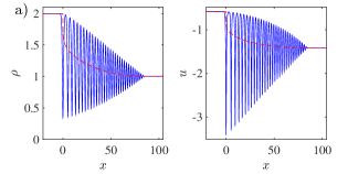
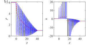
Figure 14: NLS 2-DSWs (solid) and their mean values (dashed) in the soliton reference frame with (a) $\rho_{0}=2$ at $t=50$ and (b) $\rho_{0}=6$ at $t=8$ with an interior vacuum point.

NLS DSWs exhibit curious physical behavior. For example, the density at the soliton edge goes to zero (vacuum) for sufficiently large jumps. The minimum density of the traveling wave solution (2.117) for the 2-DSW modulation (3.51), (3.52) is

$$\rho_{\text{min}}=\frac{1}{4}\left(\frac{1}{2}u_{\rm l}+\sqrt{\rho_{\rm l}}-2\sqrt{\rho_{\rm r}}-r_{3}\right)^{2}.$$ (3.55)

When evaluated at the soliton edge $r_{3}\to r_{2}=u_{\rm r}+2\sqrt{\rho_{\rm r}}$, $\rho_{\text{min}}=(\sqrt{\rho_{\rm l}}-2\sqrt{\rho_{\rm r}})^{2}$, which is zero when $\rho_{\rm l}=4\rho_{\rm r}$. The existence of a vacuum or cavitation point persists for larger density jumps and its location is embedded in the interior of the wave [135]. Associated with the development of a vacuum point is a change in the direction of fluid flow relative to the soliton edge. We can see this by choosing a reference frame in which the soliton edge is stationary, e.g., $u_{\rm r}=-\sqrt{\rho_{\rm l}}<0$ for the 2-DSW. We can define a Mach number for the flow by forming the ratio of the local flow speed to the dispersionless speed of sound

$$M=\frac{|u|}{\sqrt{\rho}}.$$

In the 2-DSW soliton reference frame, the downstream flow $u_{\rm r}$ is supersonic $M_{\rm r}=\sqrt{\rho_{\rm l}}/\sqrt{\rho_{\rm r}}>1$. The upstream flow $u_{\rm l}=\sqrt{\rho_{\rm l}}-2\sqrt{\rho_{\rm r}}$ is subsonic $M_{l}=|1-2\sqrt{\rho_{\rm r}/\rho_{\rm l}}|<1$, comparable to classical shock wave flows. However, the upstream flow changes direction when $\rho_{\rm l}=4\rho_{\rm r}$, precisely when a vacuum point forms. For $\rho_{\rm l}>4\rho_{\rm r}$, the fluid is flowing into the DSW from both the downstream and upstream directions. Example 2-DSWs with and without a vacuum point are shown in Fig. 14. The local fluid speed gets very large in the vicinity of a vacuum point and is undefined at the vacuum point. However, the fluid momentum $\rho u$ is defined at the vacuum point [4].

3.3.3 Riemann problem

Now that we have constructed the two basic wave types, rarefactions and DSWs, we can consider the general Riemann initial conditions

$$\rho(x,0)=\begin{cases}\rho_{0}&x<0\\ 1&x>0\end{cases},\quad u(x,0)=\begin{cases}u_{0}&x<0\\ 0&x>0\end{cases}.$$ (3.56)

This is a two-parameter family of initial conditions $\rho_{0}>1$, $u_{0}\in\mathbb{R}$. The results for more general left and right states can be found by utilizing the Galilean $u\to u+v$, $x\to x-vt$, scaling $\rho\to A\rho$, $u\to A^{3/2}u$, $x\to Ax$, $t\to A^{-1/2}t$, and reflection $x\to-x$, $u\to-u$ symmetries of the dispersive hydrodynamic form for the NLS equation (2.111) with $v\in\mathbb{R}$, $A>0$.

Due to its bi-directionality, the NLS Riemann problem will generically result in the generation of two waves, a 1-wave and a 2-wave, each of which is either a rarefaction or DSW with an intermediate, constant state connecting them [131]. A peculiar feature of dispersive hydrodynamic systems is that the constancy of the intermediate state is required of the dispersionless or Whitham modulation equations. This means that in the latter case, the intermediate state can be oscillatory for the NLS solution itself.

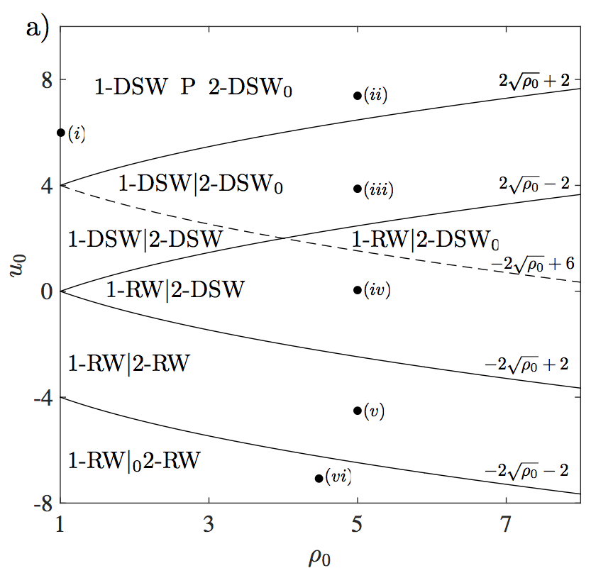
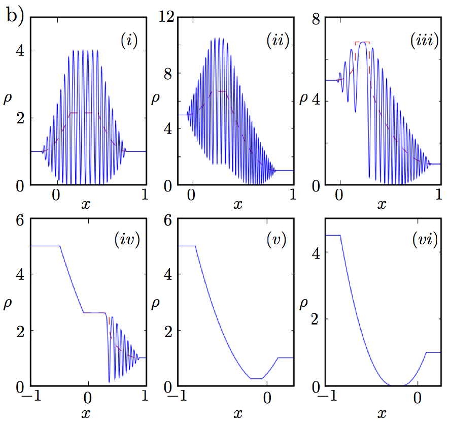
Figure 15: a) Classification of the NLS Riemann problem (3.56). (RW) - rarefaction wave; ($|$) - intermediate constant state; (P) - intermediate periodic state; zero subscript implies vacuum point. b) Modulated density (solid) and mean (dashed) for Riemann problems $(i-vi)$ identified in (a).

To determine the intermediate state $(\rho_{\rm i},u_{\rm i})$ connecting the 1- and 2-waves, we simply equate the 1-wave curve/1-DSW locus (3.46) and (3.49) to the 2-wave curve/2-DSW locus (3.47) and (3.53) according to

$$\underbrace{u_{0}+2(\sqrt{\rho_{0}}-\sqrt{\rho_{\rm i}})}_{\text{1-wave}}=u_{\rm i}=\underbrace{2(\sqrt{\rho_{\rm i}}-1)}_{\text{2-wave}}.$$ (3.57)

Solving for the intermediate state, we obtain

$$\begin{split}\rho_{\rm i}&=\frac{1}{16}\left(u_{0}+2\sqrt{\rho_{0}}+2\right)^{2},\\ u_{\rm i}&=\frac{1}{2}u_{0}+\sqrt{\rho_{0}}-1.\end{split}$$ (3.58)

Comparing the values of $\rho_{0}$ with $\rho_{\rm i}$ and $\rho_{\rm i}$ with 1 determines the type of 1- and 2-wave, respectively. For example, the dam break [133] or, equivalently, the shock tube [136] problem where $u_{0}=0$ and $\rho_{0}>1$ results in

$$\rho_{0}>\rho_{\rm i}=\frac{1}{4}(\sqrt{\rho_{0}}+1)^{2}>1,$$

implying a 1-rarefaction connected to a 2-DSW shown in Fig. 15b$iv$. The construction of this solution is depicted geometrically in Fig. 16. Blue (red) curves oriented to the left (right) are 1-wave (2-wave) curves. Since the rarefaction wave curves and DSW loci coincide, it is the direction that they are traversed that determines the wave type. The arrows point in the direction of increasing dispersionless characteristic speed for each wave family. Tracing a wave curve in the direction of increasing characteristic speed corresponds to an admissible rarefaction wave. The decreasing characteristic speed direction corresponds to an admissible DSW. We identify the solution to the Riemann problem by tracing an admissible 1-rarefaction wave curve from the left state $(\rho_{0},0)$ to the intermediate, constant state $(\rho_{\rm i},u_{\rm i})$ determined by the intersection of the 1- and 2-wave curves (3.57). Then, we follow the 2-DSW locus to the right state $(1,0)$. For more details, see [57].

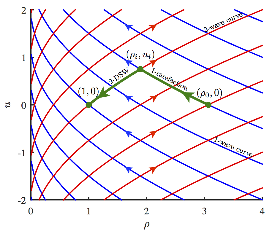
Figure 16: Traversal of 1- and 2-wave curves in solving the shock tube problem.

The classification of solutions to the NLS Riemann problem depends upon the relative ordering of the four values $r_{\pm}|_{\text{left,right}}$ and was carried out in [131]. There are five ways in which these values can be ordered, leading to five qualitatively distinct types of solutions shown in Fig. 15a,b. For sufficiently negative initial velocities, $u_{0}<-2\sqrt{\rho_{0}}+2$, there are no DSWs generated (Figs. 15b$v$,$vi$). The intermediate state (3.58) exceeds the threshold for DSW cavitation, $\rho_{\rm i}>4$, when $u_{0}>-2\sqrt{\rho_{0}}+6$. For sufficiently large initial velocities $u_{0}>2\sqrt{\rho_{0}}-2$, there are no rarefactions, only DSWs. In this regime, the 1-DSW and 2-DSW soliton edges propagate with velocities $s_{1}=u_{\rm i}+\sqrt{\rho_{\rm i}}-2\sqrt{\rho_{0}}$ (eq. (3.50)) and $s_{2}=\sqrt{\rho_{\rm i}}$ (eq. (3.54)), respectively. These velocities coincide when $u_{0}=2\sqrt{\rho_{0}}+2$. When the initial velocity exceeds this value, the intermediate state is a non-modulated, nonlinear periodic wave (Fig. 15b$ii$). The case $u_{0}>4$, $\rho_{0}=1$ leads to two counterpropagating DSWs connected by a standing periodic wave as shown in Fig. 15b$i$.

3.3.4 Piston problem

Just as the shock tube problem is a fundamental, textbook problem of classical gas dynamics, the piston problem has similar importance. Here we consider the analogous piston problem for NLS dispersive hydrodynamics. The piston problem was studied in [132, 137] with application to Bose-Einstein condensates where the action of a piston can be achieved by a repulsive laser modeled by a linear potential added to the NLS equation (2.110). This results in the Gross-Pitaevskii equation [138, 139]

$$i\psi_{t}+\frac{1}{2}\psi_{xx}+V(x,t)\psi-|\psi|^{2}\psi=0.$$ (3.59)

The piston problem also arises in the hypersonic regime of steady, two-dimensional dispersive hydrodynamic flows past an obstacle [140].

By assuming that the linear potential in the Gross-Pitaevskii equation (3.59) acts as a sharp barrier, a piston, with position $x=p(t)$, through which fluid cannot pass, it’s effect can be encapsulated by the boundary condition

$$u(p(t),t)=\dot{p}(t).$$ (3.60)

The local fluid velocity moves with the piston velocity. We follow [132] where an impulsively accelerated piston is analyzed, i.e., we assume

$$p(t)=\begin{cases}0&t<0\\ v_{p}t&t>0\end{cases},$$

where $v_{p}>0$ is the piston velocity. For a retracted piston $v_{p}<0$, the solution is a rarefaction wave, the same as in classical gas dynamics [141]. The effect of a gradually accelerated piston was described in [137].

The initial fluid profile is assumed quiescent, with normalized density

$$\rho(x,0^{-})=1,\quad u(x,0^{-})=0,\quad x>0.$$

Although we have only one boundary condition at the piston (3.60), we can formulate a uniquely solvable problem by assuming that only right-going waves in the second dispersionless characteristic field $V_{+}$, eq. (2.116), are generated, i.e., that the solution consists of a simple wave. As remarked earlier in Sec. 3.2.3, wave propagation of a quasi-linear hyperbolic system into a constant state or quiescent “gas” must occur via a simple wave [141]. Thus, we seek a 2-DSW that connects the known fluid velocity $u=v_{p}$ and some unknown density $\rho=\rho_{p}$ at the piston to the quiescent state $\rho=1$, $u=0$. The 2-DSW locus (3.53) yields the density

$$\rho_{p}=\left(\frac{1}{2}v_{p}+1\right)^{2}.$$

The velocity of the 2-DSW soliton edge $v_{s}^{-}$ and harmonic edge $v_{s}^{+}$ are therefore (3.54)

$$v_{s}^{-}=\frac{1}{2}v_{p}+1,\quad v_{s}^{+}=\frac{2v_{p}^{2}+4v_{p}+1}{v_{p}+1}.$$

This modulation solution and corresponding numerical solution are shown in Fig. 17a,c. The main quantitative difference between the modulation and numerical solutions is an overall phase shift that we have not captured in this leading order description. The slowly varying phase shift could be recovered as described for KdV modulations in Sec. 2.2.6.

The behavior observed is analogous to a piston compressing a classical gas where a shock wave is generated ahead of the piston. However, the DSW velocity exceeds the piston velocity only until $v_{p}=2$, precisely when a vacuum point appears in the DSW (3.55). Now, the oscillatory region is in contact with the piston. The boundary condition (3.60) neglected the effects of dispersion. We introduce a modification to the 2-DSW solution by imposing an alternate boundary condition to (3.60), namely that the periodic traveling wave velocity $V$ (2.118) equal the piston velocity

$$V(p(t),t)=\frac{1}{2}(r_{1}+r_{2}+r_{3}+r_{4})=v_{p}.$$ (3.61)

We continue to utilize the 2-DSW modulation (3.52) but do not require it to terminate at the soliton edge, i.e., $r_{3}>r_{2}$. Inserting the values of the known Riemann invariants (3.51) into the boundary condition (3.61), we obtain

$$r_{3}(p(t),t)=v_{p}-1,\quad v_{p}>2.$$

Since $r_{2}=1$, we observe that the solution consists of a non-modulated nonlinear, periodic traveling wave moving with the piston velocity adjacent to a partial 2-DSW. Moreover, the density minimum of the non-modulated traveling wave (2.117) is

$$\rho_{\text{min}}=\frac{1}{4}(r_{1}-r_{2}-r_{3}+r_{4})^{2}=\frac{1}{4}(v_{p}-1-r_{3})^{2}=0.$$

The amplitude of the wavetrain is

$$a=(r_{4}-r_{3})(r_{2}-r_{1})=4,$$

hence is independent of the piston velocity, once the critical value $v_{p}=2$ is exceeded. The interface between the non-modulated traveling wave and the DSW moves with speed

$$v_{s}^{-}=v_{p}+(v_{p}+3)\left[\frac{v_{p}E(m)}{(v_{p}-2)K(m)}\right]^{-1},\quad m=\frac{4}{v_{p}},$$

where $E(m)$ is the complete elliptic integral of the second kind. This modulation solution for $v_{p}=2.5$ and an associated numerical solution of (3.59) are depicted in Fig. 17b,d. It was shown that the predictions of modulation theory agree remarkably well with direct numerical simulations [132].

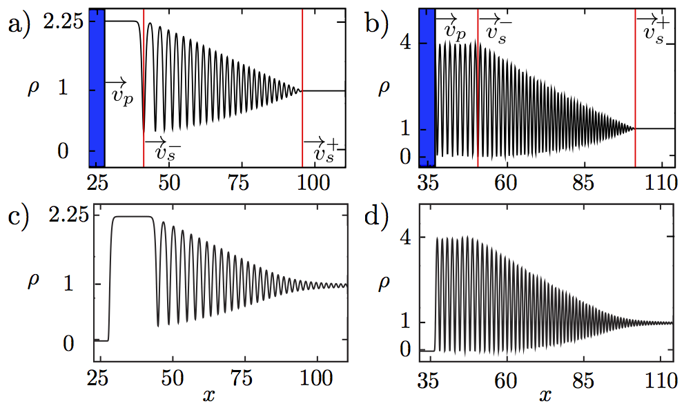
Figure 17: Modulation solutions (a,b) and numerical solutions (c,d) of the piston problem with $v_{p}=1$ (a,c) at $t=27$ and $v_{p}=2.5$ (b,d) at $t=15$. Figure adapted with permission from [132], copyrighted by the American Physical Society.

In summary, there are two dynamical regimes. The first, when $0<v_{p}<2$, is analogous to the action of a piston compressing a classical gas. A dispersive shock wave propagates ahead of the piston. The second regime, when $v_{p}>2$, has no classical correlate. Sufficiently large piston speeds compressing a dispersive fluid generate a uniform, cavitating nonlinear wavetrain at a fixed amplitude adjacent to the piston. Further downstream, this wavetrain’s amplitude becomes modulated via a 2-DSW.

3.3.5 NLS DSWs: concluding remarks

In the previous sections dedicated to defocusing NLS DSWs, we have only considered DSWs described by simple wave solutions of the modulation equations that arise due to a dispersive regularization of Riemann initial data or due to the uniform motion of a piston. Since the NLS-Whitham system (2.124), (2.125) is integrable (see Sec. 2.1.3), generalized hodograph solutions are available for it so that one can describe DSWs generated by the evolution of more general initial profiles as we did for KdV DSWs in Sec. 3.2.2. The general hodograph solution to the NLS-Whitham equations for the evolution of initially monotone profiles in $\rho$ and $u$ with a single point of wavebreaking was constructed in [135] using the method established in [106], connecting the NLS-Whitham system with the EPD system (2.98) in four-dimensional hodograph space with coordinates $r_{1},r_{2},r_{3},r_{4}$. An alternative form of this solution was obtained in [142], where a detailed study of its properties has been performed. A particular solution of the EPD system was used in [143] to describe regularization of a “cubic” wavebreaking in the NLS dispersive hydrodynamics (see Sec. 3.2.3 for the counterpart KdV problem). Also, in [143] a long-time asymptotic solution in the form of a pair of modulated dark soliton trains propagating on a constant background was obtained for the evolution of “large and smooth” initial data whose IST (Zakharov-Shabat) spectrum is domonated by a discrete component. The amplitude distributions in the soliton trains were found using a Bohr-Sommerfeld type semi-classical quantization rule for the linear spectral problem associated with the defocusing NLS equation — an analogue of the KdV soliton train distribution described in Sec. 3.2.4 (localized elevation case). A full modulation solution describing the evolution of a class of “localized” (sufficiently rapidly approaching the same non-zero constant state at $x\to\pm\infty$) initial profles was obtained in [140] in the context of hypersonic 2D superfluid flow past an airfoil (see Sec. 9.2).

Application of the NLS DSW modulation theory in the context of Bose-Einstein condensates was first considered in [144]. In [4] the NLS modulation solutions were used to identify the experimentally observed BEC blast waves (see Fig.1a,b) with DSWs. Applications of the NLS DSW modulation theory to fiber optics were discussed in [103], [114].

Concluding, we note that since the NLS equation is a generic model for the evolution of an envelope of a weakly nonlinear, quasi-monochromatic wave train, the DSWs described by the defocusing NLS equation generically represent envelope DSWs. The notion of an envelope shock (both monotone and oscillatory) was first introduced by Ostrovsky in [145] (see also [67]) in the context of weakly dissipative, dispersive systems. Such an envelope shock is described by a heteroclinic TW solution, analogous to the diffusive-dispersive shocks of the KdVB equation described in Sec. 1.3.

3.4 Focusing NLS and dispersive regularization of gradient catastrophe

The general framework of dispersive hydrodynamics (1.1) is intimately related to hyperbolicity of the dispersionless limit equation ($\mathbf{D}=0$). In the case of the defocusing NLS equation, the dispersionless limit is given by the hyperbolic shallow water equations (eq. (2.113) with $\sigma=1$). The case of the focusing NLS (fNLS) equation (eq. (2.110) with $\sigma=-1$) is very different as the dispersionless limit (2.113) is now an elliptic system, implying ill-posedness of the Cauchy problem for all but analytic initial data as discussed in Sec. 2.3.1. Ellipticity of the dispersionless limit of the focusing NLS equation is the mathematical manifestation of modulational instability of plane wave solutions, $\rho=\rho_{0},u=u_{0}$, both constants, with respect to infinitesimal perturbations. The introduction of dispersion stabilizes the propagation of short waves, as follows from the fNLS linear dispersion relation $\omega=ku_{0}\pm k(k^{2}/4-\rho_{0})^{1/2}$, which yields real values of the frequency for $k>2\sqrt{\rho_{0}}$. This observation provides a glimpse of the “partial hyperbolicity” of the modulation equations, allowing for nonlinear dispersive saturation of modulational instability via the generation of a focusing analogue of a DSW in some situations.

The periodic solutions for the focusing NLS equation (see, e.g., [54]), similar to the KdV and defocusing NLS cases, are expressed in terms of Jacobi elliptic functions with harmonic and soliton limits. Note that unlike solitons of the defocusing NLS equation, fNLS solitons have positive, “bright” polarity and exist only on a zero density, or vacuum, background. The fNLS-Whitham modulation equations have the same form as in the defocusing case (see Sec. 2.3.2) with the crucial difference that the Riemann invariants are now complex, satisfying the relations $r_{2}=r_{1}^{*}$, $r_{4}=r_{3}^{*}$, leading to complex conjugate characteristc velocities (2.126), implying the ellipticity of the modulation system. The elliptic structure of the modulation equations is the signature of nonlinear modulational instability [1, 71]. It is remarkable that, despite the elliptic structure of modulations, focusing NLS evolution can exibit highly ordered wave structures on a spatio-temporal scale $O(1)$. Some of these structures can be viewed as focusing counterparts of DSWs. The appropriate framework for the analysis of the emergence and evolution of such structures is the small-dispersion fNLS equation,

$$i\varepsilon\psi_{t}+\frac{\varepsilon^{2}}{2}\psi_{xx}+|\psi|^{2}\psi=0,\quad 0<\varepsilon\ll 1.$$ (3.62)

The evolution of (3.62) as $\varepsilon\to 0$ with analytic initial data leads to the occurrence of gradient catastrophe at some point $(x_{0},t_{0}>0)$, which represents a focusing counterpart of hyperbolic wavebreaking. Dispersive regularization of this gradient catastrophe results in the generation of rapid oscillations, which are asymptotically described by modulated solutions of the fNLS-Whitham equations. Unlike typical single-phase DSW evolution in KdV or defocusing NLS equations, the oscillations regularizing gradient catastrophe in fNLS generically have a two-phase structure and may undergo further bifurcations, giving rise to multiphase regions with the number of phases greater than two. An example of such an evolution is shown in Fig. 18. Analysis of these semi-classical structures heavily relies on the integrability of the NLS equation and typically involves a Riemann-Hilbert problem formulation of the IST (see [146, 147] and references therein; also the next section for the discussion of various relations between IST and Whitham theory).

There is a special case of focusing NLS evolution accompanied by the generation of a single-phase, modulated structure that strongly resembles a DSW in the sense that it connects two different, non-oscillating states and expands in time. This is the case of the dam break Riemann problem with a vacuum state on one side: at $t=0$, $\rho=0,u=0$ for $x>0$ and $\rho>0,u=0$ for $x<0$. An example of focusing dam break evolution into vacuum is shown in Fig. 19a. Figure 19b shows the evolution of the same dam break problem for the defocusing NLS equation, which, quite similar to the classical shallow water case, exhibits a smooth rarefaction wave [1], amended by small amplitude, dispersive oscillations of the weak discontinuities at the corners.

Dispersive regularization of the “dry bottom” dam break flow in focusing NLS is asymptotically described by modulated single-phase periodic fNLS solutions with the modulation being given by the similarity solution of the Whitham-NLS system, an analogue of the simple-wave modulation solutions of the GP problem for the KdV and defocusing NLS equations. This solution was obtained in [148] (see also [149]) and has the form

$$\begin{split}r_{1}=r_{2}^{*}=iq\\ \mathrm{Re}[V_{3}(iq,-iq,r_{3},r_{4})]=\frac{x}{t},\quad\mathrm{Im}[V_{3}(iq,-iq,r_{3},r_{4})]=0,\end{split}$$ (3.63)

where $q=\sqrt{\rho_{0}}$ and $V_{3}$ is given in (2.126). Since $V_{3}=V_{4}^{*}$, the solution (3.63) represents a double characteristic fan, a counterpart of the GP similarity solutions for the KdV- and defocusing NLS-Whitham equations (see Secs. 3.1.1, 3.3.2).

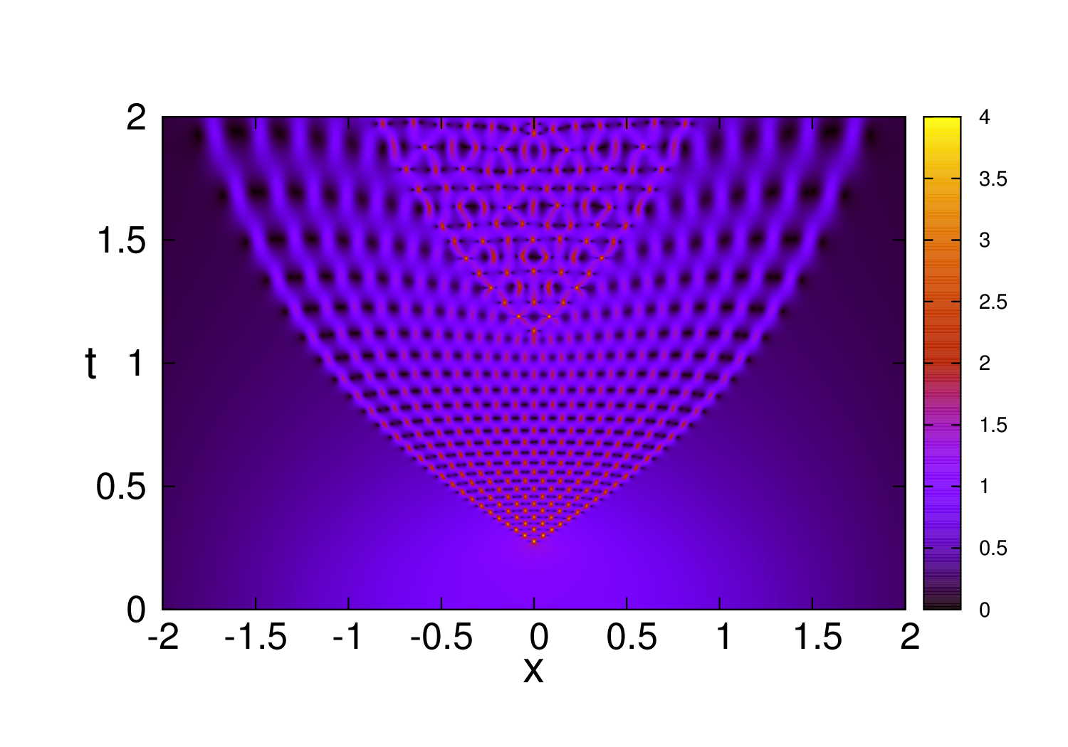
Figure 18: Contour plot of $|\psi|$ for the dispersive regularization of gradient catastrophe in the focusing NLS equation (3.62) with analytic initial condition $\psi(x,0)=\hbox{sech}\ x$ and small dispersion parameter $\varepsilon=1/33$ – numerical solution. Figure adapted, with permission, from [149].

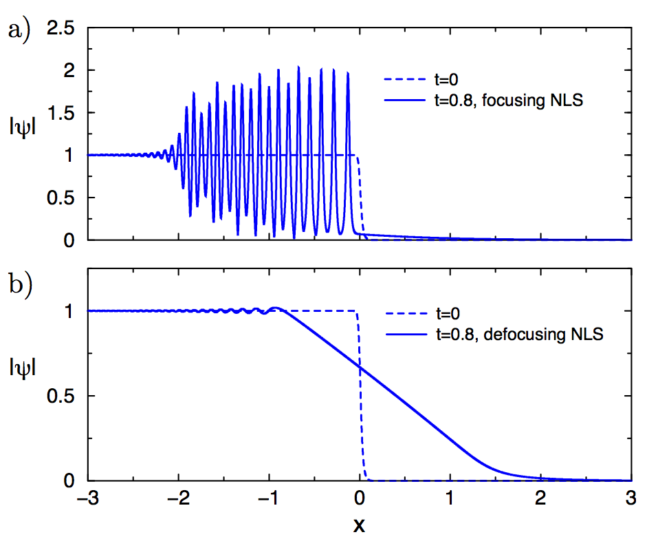
Figure 19: Dispersive regularization of the dam break problem with $\psi=0$ for $x>0$ (dashed line) in the NLS equation — numerical solution. a) focusing NLS; b) defocusing NLS.

If we let $r_{3}=a+ib$, $r_{4}=a-ib$, the solution (3.63) is represented in a particularly simple form [150, 86, 54]

$$\begin{split}\frac{x}{t}=2a+\frac{q^{2}-b^{2}}{a},\\ \frac{a^{2}+(q-b)^{2}}{a^{2}-b^{2}+q^{2}}=\frac{\mathrm{E}(m)}{\mathrm{K}(m)}\,,\quad m=\frac{4qb}{a^{2}+(q+b)^{2}}.\end{split}$$

This solution describes modulations of a single-phase wavetrain approximating the structure shown in Fig. 19a. A small amplitude two-phase modulation correction is visible but the dominant behavior is one-phase. Within the wavetrain, the modulus $m$ varies from $m=0$ at the zero-amplitude trailing edge, which propagates with the velocity $s_{-}=-2\sqrt{2\rho_{0}}$. The leading edge is given by a non-propagating soliton, $s_{+}=0$, which has amplitude $\rho_{m}=4\rho_{0}$ (note that Fig. 19 depicts $\sqrt{\rho}$).

We note that the existence of the centered, double characteristic fan solution (3.63) for an elliptic modulation system is highly non-trivial and is possible due to the special structure of the NLS-Whitham equations whose complex conjugate characteristic velocities can merge – and thus become real – on certain surfaces in the space of Riemann invariants. Recently, the modulation solution (3.63) has been recovered by a rigorous, Riemann-Hilbert problem analysis of the semi-classical NLS square barrier problem [151]. The direct IST analysis of the asymptotic development of a rather generic localized perturbation of a plane wave in [152] showed that this self-similar modulation of a single-phase, elliptic fNLS solution provides a universal asymptotic description of the nonlinear stage of modulational instability.

3.5 Modulation theory vs IST

The Inverse Scattering Transform and Whitham modulation theory are two major mathematical approaches for describing nonlinear dispersive waves. Both methods were formulated in the mid 1960s and have since been extensively used in various applications. Each of these methods has its own merits and limitations. DSW theory for KdV and other integrable equations is the common territory for both methods, hence in this section we briefly outline some prominent interrelations between them.

As we have already seen, there are several important connections between IST and Whitham theory. Firstly, the Whitham equations were shown to describe the slow evolution of finite-band IST spectrum of traveling waves (Sec. 2.2.4). Secondly, the long-time asymptotic evolution of decaying initial profiles described by modulation solutions were shown in Sec. 3.2.4 to be consistent with results from IST. However, there still remains a conceptual gap between the initial value problem for the small-dispersion KdV equation (3.14) and the GP matching problem (3.19) for the Whitham equations. Indeed, despite convincing evidence of the validity of the GP approach (mostly numerical, see, e.g., [108]), the ascertainment of its rigorous justification remained open for a good number of years. The decisive step was made in the seminal works of Lax and Levermore [50] and Venakides [153] who used the IST to study the zero dispersion limit of the solution to the initial value problem (3.14). By considering an approximation of the initial data $u_{0}(x)$ by a $N$-soliton solution, with $N\sim\varepsilon^{-1}\gg 1$, then passing to the limit as $N\to\infty$, Lax and Levermore derived the Whitham equations as equations describing the weak limits of rapidly oscillating KdV solutions generated beyond the wavebreaking point of the dispersionless limit (Hopf equation) solution (3.15). Venakides [153] extended the Lax-Levermore results to solitonless potentials, the localized depression case in terms of the initial value problem (3.14), and further, to the periodic case [154]. Additionally, Venakides bridged the Lax-Levermore [50] and FFM [61] results by revealing the generation mechanism of rapid oscillations in small-dispersion solutions [155] and later showing in [156] that higher-order corrections to the Lax-Levermore weak limits describe locally periodic or quasi-periodic oscillatory structure of the nonlinear wavepackets assumed in the FFM work. Finally, a comprehensive approach to KdV with decaying initial conditions in the small dispersion regime was developed by Deift, Venakides and Zhou (DVZ) [157] who employed the powerful nonlinear steepest descent method for the oscillatory Riemann-Hilbert problem associated with semi-classical inverse scattering introduced earlier by Deift and Zhou [158]. The DVZ analysis provides strong, pointwise asymptotics of the small-dispersion KdV solution and yields the modulation solution as part of the full information about the evolution.

The above works on rigorous IST analysis of KdV evolution have the inherent constraint of rapidly decaying initial data as $|x|\to\infty$. The IST approach was extended to non-decaying step-like initial conditions by Khruslov [110] who explained the apparent contradiction between the absence of discrete spectrum in the KdV step problem and the appearance of solitons at the DSW leading edge in the GP solution. He showed that the soliton state at the leading edge is realized only asymptotically as $t\to\infty$. Further development in the application of IST to the KdV step problem can be found in [159]. These results have recently been refined [160]. Ablowitz and Baldwin [109] employed a combination of IST with matched asymptotic expansions to study the KdV equation with “multi-step” initial data. Apart from providing the detailed structure of the solution at all times, the important conceptual result of [109] is that the long-time asymptotic state in the multistep KdV problem is a single DSW connecting the asymptotic leftmost and rightmost states. A similar result was obtained within the modulation theory approach in [161] and [162], for smooth initial data with several wavebreaking points. This result also correlates with the classical result of viscous shock merger in the overtaking interaction of two shock waves [1]. See Sec. 6 for further details.

The development of IST theory for the defocusing NLS equation with non-zero boundary conditions has been the subject of several recent works including [163] and [164]. The latter paper utilizes the Deift-Zhou Riemann-Hilbert problem approach to study the regularization of initial sharp step data for the semi-classical defocusing NLS equation and, in particular, provides rigorous justification for some of the modulation theory solutions obtained earlier in [131] (see Section 3.3.3). The connection of IST for the semi-classical focusing NLS with modulation theory has been briefly touched upon in Sec. 3.4.

We conclude this section by highlighting the key advantages, particularly for physical applications, of the modulation theory approach to the description of a DSW over fully rigorous, but also more restrictive, IST related techniques. DSW modulation theory: (i) does not impose any global limitations (rapid decay as $|x|\to\infty$ or periodicity in $x$) on the solutions; ii) provides a universal mathematical framework for DSW study within the well developed theory of quasilinear hyperbolic systems, which is greatly enhanced by the availability of Riemann invariants and the generalized hodograph transform [60]; (iii) directly yields all the key physical macroscopic DSW parameters (e.g., the amplitude and the wavelength distributions, the speeds of the edges) not readily available via IST. Most importantly, modulation theory can be applied to non-integrable systems [48], although without the advantage of having Riemann invariant structure for the modulation system, which is of crucial importance for applications. The development of DSW theory for non-integrable dispersive hydrodynamic systems will be described in the next section.

4 DSWs in non-integrable systems

So far, the emphasis in this review has been upon completely integrable equations, which predictably yield a very detailed mathematical description. As is often the case, integrable systems provide insight into fundamental processes that carry over to other systems, which are not integrable but have greater physical relevance. In particular, there has been strong numerical evidence that such fundamental features of dispersive hydrodynamics as the formation of oscillatory regions and weak convergence are true for systems that are not completely integrable but are structurally similar [165, 123]. In particular, a detailed numerical study of the Riemann problem for a system describing the dynamics of a two-temperature collisionless plasma [166] revealed that the qualitative features of KdV DSWs hold true for ion-acoustic DSWs of finite amplitude, while quantitatively there are significant differences. In particular, the qualitative DSW structure has been numerically observed to be a modulated nonlinear wavetrain with a solitary wave at one edge and a harmonic, small-amplitude wave packet at the other.

In contrast to IST, which is applicable only to integrable systems, the Whitham method of slow modulations is much more general, applicable to equations satisfying modest conditions [48]. In what follows, we utilize Whitham theory in order to describe DSWs in a number of apparently non-integrable equations. One important benefit of this generalization is the ability to accurately model more physical systems. We demonstrate this with several modern applications.

4.1 DSW fitting method

As described in Sec. 2.2, the applicability of the Whitham method [48] to a dispersive hydrodynamic system of $N$th order requires the existence of a $N$-parameter family of periodic solutions and the availability of $N-1$ local conservation laws. These requirements are satisfied by many physically relevant dispersive hydrodynamic systems. Prominent examples include systems describing ion-acoustic and magnetoacoustic waves of finite amplitude in collisionless plasma [66, 48], the Serre (Green-Naghdi, Su-Gardner) equations for fully nonlinear shallow water waves [167, 168, 169] and various versions of the generalized NLS equation, e.g., the NLS equation with saturable nonlinearity describing light propagation in photorefractive crystals [170].

The modulation systems for ion-acoustic and magnetoacoustic waves in collisionless plasma were derived in [111] and were shown to share a number of basic properties with KdV and NLS modulation systems, despite the apparent absence of Riemann invariant structure. Specifically, these systems were shown to admit exact reductions to the dispersionless limit of the original equations. Similar to the KdV and NLS cases, these reductions could be achieved either via the zero-amplitude $a\to 0$ or zero-wavenumber $k\to 0$ limit. As these two limiting regimes correspond to the DSW edges, the availability of such reductions opens up the possibility of formulating the GP matching problem.

It was shown in [56] (see also [171, 172]) that the generic structure of modulation systems in the linear and soliton limits prescribes the DSW fitting relations for a broad class of dispersive hydrodynamic systems. These DSW fitting relations are dispersive hydrodynamic counterparts of the Rankine-Hugoniot conditions of viscous shock theory and hence enable one to classify solutions of dispersive Riemann problems. In the general bi-directional case, the DSW fitting relations include: (i) the DSW locus relating admissible upstream and downstream flow states; (ii) the speeds of the DSW edges; (iii) the causality conditions determining the DSW orientation. The causality conditions are analogues of the Lax entropy inequalities in viscous shock theory. In the uni-directional case, the DSW locus does not arise. Remarkably, the DSW fitting method does not require knowledge of the full simple-wave modulation solution–although it assumes its existence–and thus circumvents a major difficulty in the analytical treatment of non-integrable systems.

The mechanisms and conditions for the breakdown of the DSW fitting construction were identified in [35, 57]. In what follows, we shall provide a brief exposition of the results of [56] and [57], which will then be applied to several physically relevant systems.

4.1.1 Scalar equations

We start with a general scalar, model equation

$$u_{t}+f(u)_{x}+D_{2}[u]_{x}=0$$ (4.1)

with $f^{\prime\prime}(u)\neq 0$ and $D_{2}$ a conservative dispersive operator of the second order so that equation (4.1) has a real-valued linear dispersion relation $\omega=\omega_{0}(k)$ with the long-wave expansion

$$\omega_{0}(k)=c_{0}k+\mu k^{3}+o(k^{3}),\quad k\ll 1,\quad\mu\neq 0,$$ (4.2)

for small-amplitude waves $\sim e^{i(kx-\omega t)}$, propagating on the background $u=u_{0}$ so that $c_{0}=f^{\prime}(u_{0})$. We shall be assuming that the dispersion relation is purely convex or concave, so that $\partial_{kk}\omega_{0}\neq 0$. Equation (4.1) fits into the general category of uni-directional dispersive-hydrodynamic systems (1.2).

We shall consider the evolution of Riemann step initial data $u(x,0)=u_{\pm}$, $\pm x>0$ (3.1) for uni-directional dispersive hydrodynamics (4.1). Our consideration will be based upon the fundamental assumption that the initial step is resolved into a DSW that has the structure of a modulated single-phase wavetrain. This assumption is exactly the one already employed in the GP modulation regularization for the KdV and NLS equations (see Secs. 3.1 and 3.3). Unlike in the integrable case, there is no method at present to rigorously confirm this assumption, so direct numerical confirmation is essential. The assumption is rooted in Whitham’s fundamental proposition that, by analogy with linear dispersive wave theory, modulated nonlinear wavetrains represent the generic, long-time outcome of a broad range of dispersive-hydrodynamic problems [1]. Our aim is to determine analytically the macroscopic DSW properties. In particular, we seek the speeds of the trailing and leading edges $s_{\pm}$ in a general form, using only basic information provided by equation (4.1). The speeds $s_{\pm}$ are the dispersive counterpart of the classical Rankine-Hugoniot relation determining the viscous shock speed. In contrast to classical shock theory, where the shock speed is determined by the hyperbolic structure alone and viscosity only modifies the transition width/shape, in dispersive hydrodynamics, the DSW speeds are determined by both the hyperbolic and dispersive structure of the equation. With the DSW speeds $s_{\pm}$ in hand, additional macroscopic DSW properties can be deduced by identifying the edge speeds with the soliton amplitude-speed relation and the group velocity, yielding the DSW soliton edge amplitude and harmonic edge wavenumber.

Suppose equation (4.1) has a three-parameter periodic traveling wave solution and at least two local conservation laws. These requirements are quite generic and are satified for a majority of dispersive hydrodynamic equations (4.1) arising in applications. Then equation (4.1) is amenable to Whitham averaging (2.27), (2.28), which yields a system of three quasilinear equations for slow variations of the traveling wave parameters. The fundamental difference from the KdV and NLS cases is that now the modulation system is unlikely to have Riemann invariants so the expressions for simple-wave solutions involve integration of the full Whitham equations. Anyway, they are not of much use for our task of identifying a generic DSW fitting description. In the absence of Riemann invariants, it is convenient to choose physical parameters as modulation variables, e.g., the period-mean $\overline{u}$, the wavenumber $k$, and the amplitude $a$.

Let the periodic traveling wave solution to (4.1), $u=\tilde{u}(\theta)$, $\theta_{x}=k$, $\theta_{t}=-\omega$, be specified by an ODE

$$k^{2}(u_{\theta})^{2}=G(u),\quad u(\theta+2\pi)=u(\theta),$$ (4.3)

where we have omitted the tilde for $u$, assuming from now on that $u$ is the traveling wave solution $u(\theta)$, rather than the general field $u(x,t)$. Let the “potential” function $G(u)$ have exactly three real roots, say $b_{1}\leq b_{2}\leq b_{3}$ where

$$G(u)=(b_{1}-u)(b_{2}-u)(b_{3}-u)H(u),$$ (4.4)

where $H(b_{i})\neq 0$, $i=1,2,3$. To be definite, we assume that $H(u)>0$ so that $G(u)$ has a graph similar to the KdV cubic potential depicted in Fig. 6 and $b_{2}\leq u\leq b_{3}$. Then the wavenumber $k$ and the wave amplitude $a$ are expressed in terms of ${\mathbf{b}}$ by (cf. (2.48), (2.49))

$$k=\pi\left(\int\limits_{b_{2}}^{b_{3}}\frac{\,\mathrm{d}u}{\sqrt{G(u)}}\right)^{-1},\quad a=b_{3}-b_{2}.$$ (4.5)

The period average of $\mathcal{F}[u]$ is defined by (cf. (2.47))

$$\overline{\mathcal{F}[u]}=\frac{k}{\pi}\int\limits^{b_{3}}_{b_{2}}\frac{\mathcal{F}[u]}{\sqrt{G(u)}}\,\mathrm{d}u,$$ (4.6)

In particular, the wave mean $\overline{u}$ is defined by eq. (4.6) with $\mathcal{F}[u]=u$. We also define the conjugate wavenumber

$$\tilde{k}=\pi\left(\int\limits_{b_{1}}^{b_{2}}\frac{\,\mathrm{d}u}{\sqrt{-G(u)}}\right)^{-1}.$$ (4.7)

When $b_{2}\to b_{1}$, the potential $G(u)$ develops a double root and the wavenumber integral in eq. (4.5) is logarithmically singular so that $k\to 0$. In this limit, $a=b_{3}-b_{1}=O(1)$ and

$$\begin{split}\lim_{b_{2}\to b_{1}}\int\limits_{b_{1}}^{b_{2}}\frac{\,\mathrm{d}u}{\sqrt{-G(u)}}=\frac{\pi}{\sqrt{(b_{3}-b_{1})H(b_{1})}},\end{split}$$

so that $\tilde{k}=O(1)$. For the same reason, when $a\to 0$, $\tilde{k}\to 0$, and $k=O(1)$. Therefore, $\tilde{k}$ is an amplitude type variable. The introduction of $\tilde{k}$ instead of $a$ as a modulation variable is advantageous because $\tilde{k}$ provides symmetry in the description of the linear and soliton regimes. Now, $k=0$ at the DSW soliton edge and $\tilde{k}=0$ at the harmonic edge. We also note that if $b_{1}\leq u\leq b_{2}$, i.e., $H(u)<0$ in (4.4), then the definitions of $k$ and $\tilde{k}$ should be simply swapped.

The full nonlinear dispersion relation $\omega(k,\overline{u},\tilde{k})$ can be determined as follows. Given $k$, $\overline{u}$, $\tilde{k}$, the three roots $\{b_{j}\}_{j=1}^{3}$ can be determined from (4.5), (4.6), (4.7) assuming a nonzero Jacobian. The phase velocity $V$, as any other parameter in the traveling wave, is determined by $\{b_{j}\}_{j=1}^{3}$, hence, in principle, the dependence of $V$ on $k,\overline{u},\tilde{k}$ is available. The nonlinear dispersion relation is then found from $\omega=kV$.

Let us now formulate the GP matching conditions for a DSW modulation solution of equation (4.1) (cf. (3.19)):

$$\begin{array}[]{l}x=x_{\rm h}(t):\qquad\tilde{k}=0\,,\ \ \overline{u}=u_{\rm h}\,,\\ x=x_{\rm s}(t):\qquad k=0\,,\ \ \overline{u}=u_{\rm s}\,,\end{array}$$ (4.8)

where the subscripts ‘h’ (harmonic) and ‘s’ (soliton) are associated with the DSW edges. One has either $({\rm h},{\rm s})=(-,+)$ or $({\rm h},{\rm s})=(+,-)$, depending on the DSW orientation $d$, which is unknown at the outset and will be determined by an analogue of the entropy condition (see Sec. 3.1). If $d=1$, then $({\rm h},{\rm s})=(-,+)$, i.e., the trailing edge is associated with harmonic vanishing amplitude waves and the leading edge with a solitary wave. If $d=-1$, the edge association is opposite.

The edges $x_{{\rm h},{\rm s}}(t)$ are determined by the kinematic conditions (cf. conditions (3.21) for the KdV case)

$$\frac{dx_{\rm h}}{dt}=\partial_{k}\omega(k_{\rm h},u_{\rm h}),\quad\frac{dx_{\rm s}}{dt}=\tilde{V}_{s}(\tilde{k}_{\rm s},u_{\rm s}),$$ (4.9)

where $\tilde{V}_{s}(\tilde{k},\bar{u})=V_{s}(a_{s}(\tilde{k},\bar{u}),\bar{u})$ is the soliton amplitude-speed relation re-written in terms of $\tilde{k}$. We note that for each specific case, the identification of the harmonic edge velocity with the linear group velocity and the soliton edge with the soliton amplitude-speed relation can be deduced from an asymptotic analysis of the characteristic velocities of the modulation equations, which can be done for small amplitudes or small wavenumbers. Alternatively, conditions (4.9) can be generically postulated using the properties of linear and solitary waves [1].

We now represent the modulation system, obtained by averaging two conservation laws and complemented by wave conservation $k_{t}+\omega_{x}=0$, in the general form of a quasilinear system (2.1) (c.f. (2.29))

$${\bf U}_{t}+\mathrm{A}({\bf U}){\bf U}_{x}=0\,,$$ (4.10)

where ${\bf U}({\bf x},t)=(\bar{u},k,\tilde{k})^{T}$ and $\mathrm{A}(\mathbf{U})$ is the Jacobian matrix. Our major assumption is that the modulation system (4.10) is strictly hyperbolic and genuinely nonlinear, which guarantees the existence of self-similar solutions compatible with the Riemann data (3.1). Later, we shall present a simple analytic criterion for the breakdown of genuine nonlinearity of the modulation system in the context of DSW theory.

Due to the form of the potential $G(u)$ (4.4), an asymptotic calculation of (4.6) in both harmonic ($\tilde{k}=0$) and soliton ($k=0$) limits, we have $\overline{\mathcal{F}[u]}=\mathcal{F}[\overline{u}]$. Then, for example, in the harmonic limit the modulation system assumes the form

$$\begin{split}\tilde{k}=0,\ \ {\overline{u}}_{t}+V({\overline{u}}){\overline{u}}_{x}=0,\ \ k_{t}+\omega_{0}(k,{\overline{u}})_{x}=0,\end{split}$$ (4.11)

where $V(u)=f^{\prime}(u)$ and $\omega_{0}(k,{\overline{u}})$ is the linear dispersion relation obtained by the linearization of (4.1) against the background state $u={\overline{u}}$. The exact reduction (4.11) has been deduced directly from the full modulation system of (4.1) but it can be convincingly postulated on the “physical” grounds that in the harmonic, zero amplitude limit, the modulation equation for the mean must agree with the dispersionless limit equation, while the wave conservation equation is generic.

A similar reduction of the modulation system to just two equations exists in the opposite, zero wavenumber case. The derivation of this reduction, however, is more subtle than in the zero-amplitude case as the limit $k\to 0$ is a singular one for the wavenumber conservation law (see [171, 56] for details).

We shall now look at how the reduced system (4.11) and its zero-wavenumber counterpart can characterize the similarity solution of the full modulation system (4.10), describing DSW evolution for the Riemann problem. Let the characteristic velocities of (4.10) be ordered as $V_{1}\leq V_{2}\leq V_{3}$. It can then be concluded that the required modulation solution is associated with the 2-wave integral curve, (cf. (3.6) in the KdV case)

$$V_{2}=s=\frac{x}{t},\quad I_{1}(\overline{u},k,\tilde{k})=0,\quad I_{2}(\overline{u},k,\tilde{k})=0,$$ (4.12)

where $I_{1},I_{2}$ are the characteristic integrals of (4.10) associated with the simple-wave solution and correspond to fixed Riemann invariants for diagonalizable systems. The integral curve (4.12) connects two constant states of the solution vector $(\overline{u},k,\tilde{k})$: the state $(u_{\rm h},k_{\rm h},0)$ at the harmonic edge and $(u_{\rm s},0,\tilde{k}_{\rm s})$ at the soliton edge. At these endpoints of the integral curve, the merger of two of the characteristic velocities, as well as of the integrals $I_{1}$ and $I_{2}$, occurs.

While $u_{\rm h}$ and $u_{\rm s}$ are given by the initial Riemann data (modulo the DSW orientation), the parameters $k_{\rm h}$ and $\tilde{k}_{\rm s}$ are unknown. These can be determined from the condition that the DSW edges be characteristics of the modulation system (4.10), so for each of them, there is a characteristic relation (2.6) connecting the differentials of all modulation variables: $d\overline{u}$, $dk$ and $d\tilde{k}$ (see (2.7)). For the limiting cases $\tilde{k}=0$ and $k=0$, these characteristic relations, and therefore the integrals $I_{1}$ and $I_{2}$ in (4.12), can be found directly from the reduced modulation systems. For example, along the harmonic edge $d\tilde{k}=0$ and so the relevant characteristic relation connects only $dk$ and $d\overline{u}$, implying $k=k(\overline{u})$. Substituting this into the zero-amplitude reduction system (4.11) immediately yields the characteristic ODE for the harmonic edge

$$\frac{\,\mathrm{d}k}{\,\mathrm{d}\overline{u}}=\frac{\partial\omega_{0}/\partial{\bar{u}}}{V({\bar{u}})-\partial\omega_{0}/{\partial k}},\quad k(u_{\rm s})=0\,.$$ (4.13)

The initial condition for the harmonic edge ODE (4.13) is found from the GP matching condition (4.8) at the opposite, soliton edge. Indeed, this GP condition does not contain $\tilde{k}$ and thus must be valid for all $\tilde{k}$ including $\tilde{k}=0$. Said differently, the characteristic integrals (4.12) must hold for all $\tilde{k}$. One of them, say $I_{1}$, determines the integration constant for the simple wave $k=k(\bar{u})$ along the harmonic edge via $I_{1}(u_{\rm s},0,\tilde{k}_{\rm s})=I_{1}(u_{\rm s},0,0)=0$. The solution $k({\overline{u}})$ of (4.13) determines the value of $k_{\rm h}=k(u_{\rm h})$ at the harmonic edge. Then, since the harmonic edge propagates with the linear group velocity (see (4.9)), one has $s_{\rm h}=\partial_{k}\omega_{0}(k_{\rm h},u_{\rm h})$.

An analogous consideration of the soliton edge leads to the ODE for $\tilde{k}$ (the derivation, however, is less straightforward than for the harmonic edge, see [56]),

$$\frac{\,\mathrm{d}\tilde{k}}{\,\mathrm{d}\overline{u}}=\frac{\partial\tilde{\omega}_{0}/\partial{\overline{u}}}{V({\bar{u}})-\partial\tilde{\omega}_{0}/{\partial\tilde{k}}},\quad\tilde{k}(u_{\rm h})=0,$$ (4.14)

where $\tilde{\omega}_{0}(\tilde{k},\overline{u})=-i\omega_{0}(i\tilde{k},\bar{u})$ is the conjugate dispersion relation. Integrating (4.14), we determine the value of $\tilde{k}$ at the soliton edge. The velocity of the soliton edge coincides with the soliton velocity, defined as $V_{\rm s}=\lim_{k\to 0}\omega/k$, where $\omega$ is the nonlinear traveling wave frequency. It can then be shown [56] that $V_{\rm s}=\tilde{\omega}_{0}/\tilde{k}$. Then the soliton edge velocity, see the second expression in (4.9), is found as $s_{\rm s}=\tilde{\omega}_{0}(\tilde{k}_{\rm s},u_{\rm s})/\tilde{k}_{\rm s}$, where $\tilde{k}_{\rm s}=\tilde{k}(u_{\rm s})$.

Now we will identify the harmonic (h) and soliton (s) edges with the leading or trailing edge propagation with the speeds $s_{+}$ and $s_{-}$ respectively. This is done by choosing a DSW orientation, i.e., by identifying $s_{\rm s}$ and $s_{\rm h}$ with $s_{+}$ and $s_{-}$ and verifying the causality conditions,

$$s_{-}<V(u_{-}),\ \ s_{+}>V(u_{+}),\ \ s_{+}>s_{-},$$ (4.15)

ensuring that the external characteristic family $\,\mathrm{d}x/\,\mathrm{d}t=V(u)$ carries data into the DSW region (cf. Fig. 10). If the inequalities are not satisfied, it is necessary to change the DSW orientation. We stress that the correct choice of the DSW orientation is a necessary, but generally not sufficient condition for the fulfillment of the causality conditions.

Example

As an example of the application of the DSW fitting method, we recover the results of the modulation analysis of the KdV Riemann problem without invoking the Riemann invariant structure. The KdV (2.33) dispersion relation is $\omega_{0}=k\bar{u}-k^{3}$, and the hyperbolic velocity $V(\bar{u})=\bar{u}$. Then the ODE (4.13) readily yields $k=\sqrt{\tfrac{2}{3}(\bar{u}-u_{\rm s})}$. Similarly, from (4.14) we obtain $\tilde{k}=\sqrt{\tfrac{2}{3}(u_{\rm h}-\bar{u})}$.

Now, $k_{\rm h}=\tilde{k}_{\rm s}=\sqrt{\tfrac{2}{3}(u_{\rm h}-u_{\rm s})}$ implying $u_{\rm h}>u_{\rm s}$. Let $\Delta=u_{\rm h}-u_{\rm s}>0$. Then, for the harmonic edge we have $s_{\rm h}=\omega_{k}(k_{\rm h},u_{\rm h})=u_{\rm h}-3k_{\rm h}^{2}=u_{\rm s}-\Delta$. For the soliton edge we use $\tilde{\omega}_{0}=\tilde{k}\bar{u}+\tilde{k}^{3}$, giving $s_{\rm s}=u_{\rm s}+\tilde{k}_{\rm s}^{2}=u_{\rm s}+\frac{2}{3}\Delta$. Then the condition $u_{\rm h}>u_{\rm s}$ implies $s_{\rm s}>s_{\rm h}$, which yields the orientation $d=1$. Hence $u_{\rm s}\equiv u_{+}$ and $u_{\rm h}\equiv u_{-}$ and $s_{+}=s_{\rm s}$, $s_{-}=s_{\rm h}$ as in (3.7), (3.8). One can see that the causality conditions (4.15) are satisfied, being, in the KdV case, equivalent to the single condition $u_{-}>u_{+}$.

In order for this simple wave DSW construction to hold, we require monotonicity of the characteristic velocity $V_{2}$ as the 2-wave curve is traversed (recall Sec. 2.1.2) or, equivalently, genuine nonlinearity of the Whitham modulation system (4.10). This requirement places restrictions on the dispersive and nonlinear properties of the governing equation (4.1). In particular, the assumption of the existence of a simple wave modulation solution implies

$$\frac{\,\mathrm{d}V_{2}}{\,\mathrm{d}\bar{u}}=\frac{\partial V_{2}}{\partial\bar{u}}+\frac{\partial V_{2}}{\partial\bar{k}}\frac{\partial k}{\partial\bar{u}}+\frac{\partial V_{2}}{\partial\tilde{k}}\frac{\partial\tilde{k}}{\partial\bar{u}}\neq 0.$$ (4.16)

Without integrability, the direct verification of (4.16) is in general quite difficult. However, the exact reduction (4.11) at the harmonic edge and the corresponding reduction at the soliton edge enable the verification of genuine nonlinearity in the vicinity of the DSW trailing and leading edges [35]. Near the harmonic edge, the characteristic velocity is $V_{2}=\partial_{k}\omega_{0}(k_{\rm h},u_{\rm h})+\mathcal{O}(\tilde{k}^{2})$. This and (4.13) simplify (4.16) to

$$\left.\partial_{k\bar{u}}\omega_{0}\left(V-\partial_{k}\omega_{0}\right)+\partial_{kk}\omega_{0}\partial_{\bar{u}}\omega_{0}\right|_{k_{\rm h},u_{\rm h}}\neq 0.$$ (4.17)

Similarly, for the soliton edge

$$\left.\partial_{\bar{u}}\left(\frac{\tilde{\omega}_{0}}{\tilde{k}}\right)\left(V-\partial_{\tilde{k}}\tilde{\omega}_{0}\right)+\partial_{\tilde{k}}\left(\frac{\tilde{\omega}_{0}}{\tilde{k}}\right)\partial_{\bar{u}}\tilde{\omega}_{0}\right|_{\tilde{k}_{\rm s},u_{\rm s}}\neq 0.$$ (4.18)

Inequalities (4.17) and (4.18) are necessary conditions for the existence of a simple wave modulation solution. The point at which either of these criteria do not hold corresponds to an extrema in $s_{\rm h}$ or $s_{\rm s}$ as the right or left state is varied.

It has been observed that an additional restriction on the DSW fitting procedure is the convexity (or concavity) of the linear dispersion relation, $\partial_{kk}\omega_{0}\neq 0$ [35, 173, 174]. There are two known implications of a zero dispersion point $\partial_{kk}\omega_{0}=0$. Due to the well-known Benjamin-Feir-Lighthill criterion [71], the change in sign of dispersion $\mathrm{sgn}\,(\partial_{kk}\omega_{0})$ can lead to modulational instability. At the level of the Whitham equations, this implies a change of type from hyperbolic to elliptic [1]. Physically, this can be understood as a lack of well-ordered waves within the DSW. At the soliton edge, $k=0$, whereas at the harmonic edge $k=k_{\rm h}>0$. If the group velocity exhibits an extremum for some nonzero $k$ between 0 and $k_{\rm h}$, then the DSW can experience an internal collision of waves or “implosion” as has been observed in a model of magma dynamics [35] (see also Sec. 4.2.1). This manifests as a two-phase modulation region adjacent to the DSW. Another example accompanying the existence of a zero dispersion point is a linear resonance where small amplitude radiation is shed from the large amplitude soliton edge whose velocity is coincident with the linear phase velocity [173, 174].

Concluding this section, we make two important remarks. The DSW orientation is determined by the sign of dispersion, $d=-\mathrm{sgn}\,(\partial_{kk}\omega_{0})$. Indeed, the sign of dispersion determines the oscillation ordering in the DSW. For example, in media with negative dispersion, waves with smaller $k$ propagate faster, hence the DSW structure exhibits a leading soliton edge and trailing harmonic edge. Thus DSW orientation can be assumed at the very beginning of the DSW fitting construction and verified a posteriori. The second remark concerns DSW polarity and the amplitude of the edge soliton. Let’s assume $d=1$, so that we are describing the leading edge soliton. The DSW polarity coincides with the polarity of the lead soliton and is readily inferred from a qualitative analysis of the traveling wave equation (4.3). For example, if the potential function has the form (4.4) and $G(u)>0$ for $b_{2}<u<b_{3}$, then the polarity is $p=1$ (cf. Fig. 6b). If $G(u)>0$ for $b_{1}<u<b_{2}$, then $p=-1$. For $p=1$, the soliton amplitude $a_{+}$ is determined from the condition $s_{+}=V_{\rm s}(u_{+},a_{+})$, where $V_{\rm s}(\bar{u},a_{\rm s})$ is the speed-amplitude relation for solitons propagating on the background $u=\bar{u}$, available via analysis of the separatrix solution of the ODE (4.3) for the soliton configuration.

4.1.2 Dispersive Eulerian systems

In the previous section, insight gleaned from the DSW GP problem for KdV was utilized in order to build a general DSW fitting method, applicable to uni-directional, dispersive hydrodynamic equations (4.1). In this section, we reflect upon DSWs for the NLS equation, presented in Sec. 3.3, in order to generalize the DSW fitting method to bi-directional dispersive Euler equations (1.3), rewritten here for convenience

$$\begin{split}\rho_{t}+(\rho u)_{x}&=D_{1}[\rho,u],\\ (\rho u)_{t}+\left(\rho u^{2}+P(\rho)\right)_{x}&=D_{2}[\rho,u].\end{split}$$ (1.3)

The general DSW fitting procedure conveyed here is based upon [56, 172, 57].

We begin the analysis by identifying some basic properties of the dispersionless $P$-system

$$\begin{split}\rho_{t}+(\rho u)_{x}&=0\\ (\rho u)_{t}+\left(\rho u^{2}+P(\rho)\right)_{x}&=0.\end{split}$$ (4.19)

The $P$-system is genuinely nonlinear when

$$\left(\rho^{2}P^{\prime}(\rho)\right)^{\prime}\neq 0,$$ (4.20)

its characteristic velocities are

$$V_{\pm}=u\pm c(\rho)=u\pm\sqrt{P^{\prime}(\rho)},$$

and it is diagonalized by the Riemann invariants

$$r_{\pm}=u\pm\int\frac{c(\rho)}{\rho}\,\mathrm{d}\rho,$$ (4.21)

so that

$$\frac{\partial r_{\pm}}{\partial t}+V_{\pm}\frac{\partial r_{\pm}}{\partial x}=0.$$ (4.22)

Note that the definition of the Riemann invariants (4.21) differs by the factor $2$ from the definition of the analogous set (2.115) for the dispersionless cubic NLS equation. In what follows, we assume strict hyperbolicity $V_{-}<V_{+}$ and genuine nonlinearity (4.20). These are the bi-directional generalizations of nonzero flux curvature for scalar hyperbolic equations.

As is the case for the genuinely nonlinear $P$-system [41, 175] and defocusing NLS hydrodynamics (Sec. 3.3), the Riemann problem for the dispersive Euler equations (1.3) generically results in two waves separated by a constant, intermediate state. The leftmost (rightmost) wave is associated with the slower (faster) characteristic velocity $V_{-}$ ($V_{+}$) and is identified as a 1-wave (2-wave). Each wave is either a rarefaction or DSW, whose left and right states are related via a wave curve or a DSW locus.

We will make several further simplifying assumptions. We assume that the dispersive operators $D_{1,2}$ are second order and that the linear dispersion relation $\omega_{\pm}$ for the dispersive Eulerian system (1.3) has the form

$$\begin{split}\omega_{\pm}(k,\rho_{0},u_{0})=V_{\pm}(\rho_{0},u_{0})k\,\pm\,\mu k^{3}+o(k^{3}),\\ k\to 0,\quad\mu>0.\end{split}$$ (4.23)

For simplicity, we have assumed positive dispersion. The focus here will be on the “+” branch $\omega_{+}$ of the dispersion relation associated with 2-waves. In order to implement Whitham averaging on this fourth order system, we require an additional conservation law to the “mass” and “momentum” conservations associated with (1.3). Finally, we assume the existence of a four-parameter family of periodic traveling waves.

Rarefactions

Rarefaction waves are self-similar, simple wave solutions of the dispersionless $P$-system (4.19). They are integral curves (recall Sec. 2.1.2), efficiently determined from the diagonal equations (4.22). For example, a 2-rarefaction corresponds to variation in the second characteristic family associated with $V_{+}$ so that $r_{-}$ is constant throughout. The 1- and 2-wave curves are (c.f. (3.46), (3.47))

$$\textrm{1-wave curve:}\quad u_{\rm l}-u_{\rm r}=\int_{\rho_{\rm l}}^{\rho_{\rm r}}\frac{c(\rho)}{\rho}\,\mathrm{d}\rho,\quad\rho_{\rm l}>\rho_{\rm r},$$ (4.24)

$$\textrm{2-wave curve:}\quad u_{\rm l}-u_{\rm r}=-\int_{\rho_{\rm l}}^{\rho_{\rm r}}\frac{c(\rho)}{\rho}\,\mathrm{d}\rho,\quad\rho_{\rm l}<\rho_{\rm r},$$ (4.25)

where $(\rho_{\rm{l,r}},u_{\rm{l,r}})$ are the left and right states. Admissibility follows from the requirement that $V_{-}(\rho_{\rm l},u_{\rm l})<V_{-}(\rho_{\rm r},u_{\rm r})$ (1-rarefaction) and $V_{+}(\rho_{\rm l},u_{\rm l})<V_{+}(\rho_{\rm r},u_{\rm r})$ (2-rarefaction). The rarefaction wave’s spatiotemporal profile is determined by inverting, for example, $V_{+}(r_{-},r_{+}(s))=s$, $s=x/t$ for the 2-rarefaction.

DSWs

The DSW fitting method applied to the dispersive Euler system (1.3) closely follows the prescription for scalar dispersive hydrodynamic equations (4.1). The four parameter family of periodic traveling waves $\rho(x,t)=\tilde{\rho}(\theta)$, $u(x,t)=\tilde{u}(\theta)$, $\theta_{x}=k$, $\theta_{t}=-\omega$, is assumed to satisfy an ODE $k^{2}(\rho^{\prime})^{2}=G(\rho)$ where the potential $G$ has three real roots, and we have dropped the tilde for notational simplicity. The dependence of $k$ on these roots is, as usual, fixed by the condition of $2\pi$-periodicity in $\theta$ (cf. (2.48)). We invoke the “symmetric” physical parametrization $\mathbf{U}=(\overline{\rho},\overline{u},k,\tilde{k})^{T}$ consisting of the wave’s average density $\overline{\rho}$ and velocity $\overline{u}$, as well as the wavenumber $k$ and conjugate $\tilde{k}$. The four Whitham equations

$$\mathbf{U}_{t}+\mathrm{A}\mathbf{U}_{x}=0$$ (4.26)

are obtained by averaging three local conservation laws over a wave period and adjoining the conservation of waves $k_{t}+\omega_{x}=0$.

By either similar reasoning to the scalar case or hypothesis, we have that the Whitham equations (4.26) admit exact reductions to the dispersionless $P$-system (4.19) when $\tilde{k}\to 0$ (zero amplitude) and $k\to 0$. The zero amplitude reduction has the form

$$\begin{split}\overline{\rho}_{t}+(\overline{\rho}\,\overline{u})_{x}&=0\\ (\overline{\rho}\,\overline{u})_{t}+\left(\overline{\rho}\,\overline{u}^{2}+P(\overline{\rho})\right)_{x}&=0\\ \tilde{k}=0,\quad k_{t}+\left(\omega_{+}(\overline{\rho},\overline{u},k)\right)_{x}&=0,\end{split}$$ (4.27)

where we have chosen the “+” branch of the linear dispersion relation and have therefore assumed a 2-DSW. Since we have assumed positive dispersion (4.23), we expect a 2-DSW with orientation $d=-1$. Then the GP matching conditions are formulated according to

$$\begin{split}x&=s_{\rm l}t:\quad k=0,\quad\overline{\rho}=\rho_{\rm l},\quad\overline{u}=u_{\rm l},\\ x&=s_{\rm r}t:\quad\tilde{k}=0,\quad\overline{\rho}=\rho_{\rm r},\quad\overline{u}=u_{\rm r},\end{split}$$

and the edge speeds $s_{\rm{l,r}}$ are to be determined.

The DSW locus can be determined by invoking a backward characteristic argument [56], where the “dual” of a 2-DSW, resulting from negative time propagation of an initial jump from $(\rho_{\rm l},u_{\rm l})$ to $(\rho_{\rm r},u_{\rm r})$, is a 2-rarefaction (4.25). Because time has been reversed, the 2-rarefaction admissibility criterion $\rho_{\rm l}<\rho_{\rm r}$ must also be reversed. Therefore, the 2-DSW locus is

$$\textrm{2-DSW locus:}\quad u_{\rm l}-u_{\rm r}=-\int_{\rho_{\rm l}}^{\rho_{\rm r}}\frac{c(\rho)}{\rho}\,\mathrm{d}\rho,\quad\rho_{\rm l}>\rho_{\rm r}.$$ (4.28)

The causality conditions (4.15) generalize to the 2-DSW here according to

$$\begin{split}\textrm{2-DSW causality:}\quad V_{-}|_{\rm left}<s_{\rm l}<V_{+}|_{\rm left},\\ V_{+}|_{\rm right}<s_{\rm r},\quad s_{\rm r}>s_{\rm l}.\end{split}$$ (4.29)

Repeating these arguments for the 1-DSW yields

$$\textrm{1-DSW locus:}\quad u_{\rm l}-u_{\rm r}=\int_{\rho_{\rm l}}^{\rho_{\rm r}}\frac{c(\rho)}{\rho}\,\mathrm{d}\rho,\quad\rho_{\rm l}<\rho_{\rm r}.$$ (4.30)

$$\textrm{1-DSW causality:}\quad V_{-}|_{\rm right}<s_{\rm r}<V_{+}|_{\rm right},$$ (4.31)

$$\qquad\qquad\qquad\qquad s_{\rm l}<V_{-}|_{\rm left},\quad s_{\rm r}>s_{\rm l}.$$

As in the NLS case, the DSW loci correspond to inadmissible wave curves.

Returning to the 2-DSW construction, we now seek a simple wave solution of the zero amplitude reduction (4.27). This is a system of three hyperbolic equations so it is not immediately clear that we will be able to integrate it. The key is to assume a local relationship $F(\overline{\rho},\overline{u})=C_{0}$ [56]. Because it is independent of both $\tilde{k}$ and $k$, it must be valid along both the zero amplitude reduction (4.27) and the analogous zero wavenumber reduction so that $F(\rho_{\rm l},u_{\rm l})=F(\rho_{\rm r},u_{\rm r})$. In order to be consistent with the 2-DSW locus (4.28), we must have the local relation

$$\overline{u}=u_{\rm l}+\int_{\rho_{\rm l}}^{\overline{\rho}}\frac{c(\rho)}{\rho}\,\mathrm{d}\rho,$$ (4.32)

valid along both the zero amplitude and zero wavenumber reductions. Using (4.32), we can now eliminate one variable from the reduction (4.27) and obtain

$$\begin{split}\overline{\rho}_{t}+V_{+}(\overline{\rho},\overline{u}(\overline{\rho}))\overline{\rho}_{x}&=0,\quad\tilde{k}=0,\\ k_{t}+\left(\omega_{+}(\overline{\rho},\overline{u}(\overline{\rho}),k)\right)_{x}&=0,\end{split}$$

which is the same as the scalar, zero amplitude reduction (4.11). The simple wave ODE is obtained in the same manner

$$\frac{\,\mathrm{d}k}{\,\mathrm{d}\overline{\rho}}=\frac{\partial\omega_{+}/\partial\overline{\rho}}{V_{+}-\partial\omega_{+}/\partial k},\quad k(\rho_{\rm l})=0.$$ (4.33)

Upon integration of (4.33), and evaluating $k_{\rm r}=k(\rho_{\rm r})$, we can obtain the harmonic, leading edge 2-DSW speed via the group velocity $s_{\rm r}=\partial_{k}\omega_{+}(\rho_{\rm r},u_{\rm r},k_{\rm r})$.

The zero wavenumber, soliton edge is analyzed in a similar fashion (see [56] for details), leading to the simple wave ODE

$$\frac{\,\mathrm{d}\tilde{k}}{\,\mathrm{d}\overline{\rho}}=\frac{\partial\tilde{\omega}_{+}/\partial\overline{\rho}}{V_{+}-\partial\tilde{\omega}_{+}/\partial\tilde{k}},\quad\tilde{k}(\rho_{\rm r})=0,$$ (4.34)

with the conjugate frequency $\tilde{\omega}_{+}=-i\omega_{+}(\overline{\rho},\overline{u},i\tilde{k})$. Integrating (4.34) and determining $\tilde{k}_{\rm l}=\tilde{k}(\rho_{\rm l})$ yields the soliton, trailing edge 2-DSW speed $s_{\rm l}=\tilde{\omega}_{+}(\rho_{\rm l},u_{\rm l},\tilde{k}_{\rm l})/\tilde{k}_{\rm l}$. As in the scalar case, the soliton edge amplitude $a_{\rm l}$ can be determined from the soliton amplitude-speed relation.

The DSW fitting carried out here was for a 2-DSW in the presence of positive dispersion so that $d=-1$. Appropriate modifications are required for other cases, e.g., $+\to-$ in eqs. (4.33), (4.34) and usage of the 1-DSW locus (4.30) apply to a 1-DSW with negative dispersion.

Similar to the scalar case, this DSW fitting method requires additional admissibility criteria such as genuine nonlinearity of the Whitham equations and convex dispersion [57]. For the 2-DSW, we require monotonicity in the third characteristic Whitham velocity $V_{3}$, which amounts to the requirement

$$\begin{split}&\partial_{kk}\omega_{+}\partial_{\overline{\rho}}\omega_{+}\\ &+(V_{+}-\partial_{k}\omega_{+})\left(\partial_{k\overline{\rho}}\omega_{+}+\partial_{k\overline{u}}\omega_{+}\frac{c}{\overline{\rho}}\right)\Big{|}_{k_{\rm h},\rho_{\rm h},u_{\rm h}}\neq 0,\end{split}$$ (4.35)

where $(k_{\rm h},\rho_{\rm h},u_{\rm h})$ are the modulation parameters at the harmonic edge. At the soliton edge, genuine nonlinearity implies

$$\begin{split}&\partial_{\tilde{k}}\left(\frac{\tilde{\omega}_{+}}{\tilde{k}}\right)\partial_{\overline{\rho}}{\tilde{\omega}_{+}}\\ &+(V_{+}-\partial_{\tilde{k}}{\tilde{\omega}_{+}})\left(\partial_{\overline{\rho}}\left(\frac{\tilde{\omega}_{+}}{\tilde{k}}\right)+\partial_{\overline{u}}\left(\frac{\tilde{\omega}_{+}}{\tilde{k}}\right)\frac{c}{\overline{\rho}}\right)\bigg{|}_{k_{\rm s},\rho_{\rm s},u_{\rm s}}\neq 0,\end{split}$$

where $(k_{\rm s},\rho_{\rm s},u_{\rm s})$ are the modulation parameters at the soliton edge.

In summary, the DSW fitting method applied to the bi-directional dispersive Euler equations (1.3) reduces to the same simple wave ODEs as in the scalar dispersive hydrodynamic case (4.1) with the additional, local application of the DSW locus.

4.2 Applications of the DSW fitting method

We now provide several examples of the DSW fitting method applied to non-integrable dispersive hydrodynamic equations.

4.2.1 Viscous fluid conduits

When a viscous fluid is injected from below into a tall reservoir of miscible, heavier, more viscous fluid, the injected fluid buoyantly rises and eventually establishes a steady flow configuration consisting of a fluid conduit or fluid-filled pipe [176]. Due to high viscosity contrast, there is negligible drag at the interface between the two fluids. As such, the driven fluid conduit can be modeled as a deformable pipe [177]. A multiple scales, perturbation derivation leads to the conduit equation [178]

$$A_{t}+(A^{2})_{z}-(A^{2}(A^{-1}A_{t})_{z})_{z}=0,$$ (4.36)

describing long interfacial waves along the fluid conduit. The dimensionless cross-sectional area of the conduit $A$ satisfies a nonlinear, dispersive wave equation that expresses conservation of the injected fluid’s mass. The nonlinear convection term expresses the self-steepening effect of buoyancy while the nonlinear, nonlocal dispersive term expresses the effect of normal and tangential interfacial stresses.

The conduit equation is a long wave model with no amplitude assumption in its derivation. This combined with the form of the nonlinear dispersion term makes the conduit equation a scalar analogue of the Serre equations for long, shallow water waves of arbitrary height, studied in the next section. The conduit equation (4.36) happens to be one of a class of equations modeling magma migration in the Earth’s mantle [179, 180]. The viscous fluid conduit system has been used as a model system to investigate solitons experimentally [177, 181, 182, 183]. Mathematically, it falls into the class of dispersive hydrodynamic equations (4.1) amenable to the DSW fitting method.

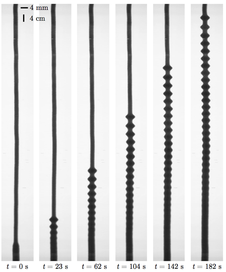
Figure 20: Viscous fluid conduit DSW formation and propagation [184]. Images have a 1:10 horizontal to vertical aspect ratio.

An example conduit DSW is pictured in Fig. 20 [184]. A narrower conduit, supported by injection at a fixed rate, is followed by a wider conduit, generated by a gradual ramp-up to a larger injection rate. This leads to a sharp transition in conduit diameter, gradient catastrophe, at $t=0$ for simplicity. The nominal jump ratio in Fig. 20 is $A_{-}/A_{+}\approx 2.9$, where $A_{\pm}$ are the leading and trailing conduit cross sectional areas, respectively. Due to interfacial dispersion, this approximate Riemann problem is resolved by the generation of a DSW.

Previous studies have described conduit DSWs in the small amplitude, long wave regime of (4.36) where the KdV equation is valid [185]. Here we follow [35] and apply the DSW fitting method to solutions of the non-integrable [186] conduit equation (4.36).

We require the linear dispersion relation for $A(z,t)=\overline{A}+ae^{i(kz-\omega t)}+c.c.$, $a\to 0$

$$\omega_{0}(k,\overline{A})=\frac{2\overline{A}k}{1+\overline{A}k^{2}},$$

and the long wave sound speed

$$c(\overline{A})=\lim_{k\to 0}\frac{\omega(k,\overline{A})}{k}=2\overline{A}.$$

The conduit equation itself is one conservation law for the system. It can be shown that the only other one is [187, 188]

$$\left(\frac{1}{A}+\frac{A_{z}^{2}}{A^{2}}\right)_{t}+\left(\frac{A_{tz}}{A}-\frac{A_{z}A_{t}}{A^{2}}-2\ln A\right)_{z}=0.$$

With this information in hand, we can apply the DSW fitting method. We consider the Riemann initial conditions

$$A(z,0)=\begin{cases}A_{0}&z<0\\ 1&z>0\end{cases},\quad A_{0}>1.$$

The scaling symmetry $A\to\overline{A}^{-1}A$, $z\to\overline{A}^{-1/2}z$, $t\to\overline{A}^{1/2}t$ satisfied by solutions of (4.36) enables more general initial jumps.

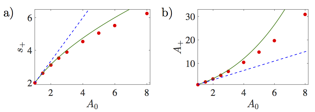
Figure 21: Conduit DSW macroscopic properties. a) Soliton edge speed versus jump height. b) Soliton edge amplitude. Numerics (circles), DSW fitting (solid), KdV approximation (dashed).

From eq. (4.13), the harmonic, trailing edge of the DSW is described by integrating

$$\frac{\,\mathrm{d}k}{\,\mathrm{d}\overline{A}}=\frac{1}{\overline{A}^{2}k(\overline{A}k^{2}+3)},\quad k(1)=0.$$

The substitution $\alpha=\overline{A}k^{2}$ gives the separable ODE

$$\frac{\,\mathrm{d}\alpha}{\,\mathrm{d}\overline{A}}=\frac{(\alpha+2)(\alpha+1)}{\overline{A}(\alpha+3)},\quad\alpha(1)=0.$$

Integration and evaluation at the trailing, harmonic edge $\overline{A}=A_{0}$ yields the wavenumber

$$k_{-}^{2}=\frac{1}{4A_{0}}\left(A_{0}-4+\sqrt{A_{0}(8+A_{0})}\right).$$ (4.37)

The harmonic edge speed is determined by evaluating the group velocity

$$s_{-}=\frac{\partial\omega_{0}}{\partial k}(k_{-},A_{0})=8+3A_{0}-3\sqrt{A_{0}(8+A_{0})}.$$ (4.38)

The soliton, leading edge of the DSW is analyzed by introducing the conjugate wavenumber $\tilde{k}$ and frequency $\tilde{\omega}$

$$\tilde{\omega}_{0}(\tilde{k},\overline{A})=-i\omega_{0}(i\tilde{k},\overline{A})=\frac{2\overline{A}\tilde{k}}{1-\overline{A}\tilde{k}^{2}}.$$

Then the soliton edge speed is found by integrating (4.14)

$$\frac{\,\mathrm{d}\tilde{k}}{\,\mathrm{d}\overline{A}}=\frac{1}{\overline{A}^{2}\tilde{k}(\overline{A}\tilde{k}^{2}-3)},\quad\tilde{k}(A_{0})=0.$$

Introducing the change of variable $\tilde{\alpha}=\overline{A}\tilde{k}^{2}$ leads to

$$\frac{\,\mathrm{d}\tilde{\alpha}}{\,\mathrm{d}\overline{A}}=\frac{(\tilde{\alpha}-2)(\tilde{\alpha}-1)}{\overline{A}(\tilde{\alpha}-3)},\quad\tilde{\alpha}(A_{0})=0.$$

Integration and evaluation at the soliton edge $\overline{A}=1$ identifies the conjugate wavenumber

$$\tilde{k}_{+}^{2}=1+\frac{\sqrt{1+8A_{0}}-1}{4A_{0}}.$$

Evaluating the phase speed gives the leading edge soliton speed

$$s_{+}=\frac{\tilde{\omega}_{0}(\tilde{k}_{+},1)}{\tilde{k}_{+}}=\sqrt{1+8A_{0}}-1.$$ (4.39)

The leading edge soliton amplitude $A_{+}$ can be determined by inverting the soliton amplitude-speed relation

$$\sqrt{1+8A_{0}}-1=\frac{A_{+}^{2}(2\ln A_{+}-1)+1}{(A_{+}-1)^{2}}.$$ (4.40)

Small jump $0<\Delta=A_{0}-1\ll 1$ expansions of (4.39) and (4.40) yield the approximate results $s_{+}\sim 2+\frac{4}{3}\Delta$, $A_{+}\sim 2\Delta$, in agreement with the KdV approximation [189, 35].

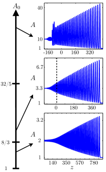
Figure 22: Numerical computation of conduit DSWs with differing jump heights. Small jump ($A_{0}=2$), the DSW is KdV-like. Moderate jump ($A_{0}=3.3$), the DSW exhibits backflow. Large jump ($A_{0}=10$), the DSW implodes. See [35].

Thus we have arrived at the relatively simple expressions (4.37), (4.38) for the harmonic edge and (4.39), (4.40) for the soliton edge macroscopic DSW properties. A comparison of macroscopic DSW properties at the soliton edge with numerical simulations of eq. (4.36) for a smoothed step are shown in Fig. 21. The KdV approximation only holds in the extremely small jump regime, demonstrating the importance of this non-integrable, DSW fitting approach. The deviation between modulation theory and numerics for large jump heights could be due to a loss of genuine nonlinearity in the full Whitham system or other causes. We consider one such possibility below.

The trailing edge speed in (4.38) can be negative when $A_{0}>8/3$. This corresponds to a negative group velocity and the development of backflow. Although the injected fluid is buoyantly rising in the column, interfacial waves are backpropagating downward. Such behavior has been observed experimentally [184] and is shown numerically in Fig. 22.

For sufficiently long waves, the dispersion

$$\frac{\partial^{2}\omega_{0}}{\partial k^{2}}(k,\overline{A})=-\frac{4\overline{A}^{2}k(3-\overline{A}k^{2})}{(1+\overline{A}k^{2})^{3}},$$ (4.41)

is negative, concave. There is an inflection point at the critical wavenumber $k^{2}=3/\overline{A}$. Inserting the expression for $k_{-}$ (4.37) into (4.41), we find that the DSW trailing edge crosses the zero dispersion point when $A_{0}=32/5$. This change in dispersion sign leads to what was termed implosion, because the waves at the trailing edge move faster than the waves in the interior of the DSW, leading to an internal two-phase interaction [35]. This behavior is due to a change of type for the Whitham equations from hyperbolic to elliptic. See Sec. 4.1.1.

The three DSW behaviors are shown in Fig. 22 as numerical simulations of a smoothed step initial condition for the conduit equation (4.36).

4.2.2 Shallow water DSWs — undular bores

One of the earliest experiments on DSWs occurred in the context of channel flow where an undular hydraulic jump or undular bore was created in 1865 by Darcy and Bazin [21, 190]. Some measurements from these experiments are depicted in Fig. 23a. A tidal bore propagating upstream in certain rivers can form when the incoming tide is strong enough. If the Froude number (ratio of the vertically averaged horizontal flow speed to the long wave speed) is larger than unity but less than 1.4 to 1.7, then the bore takes on an undular character. An example from Turnagain Arm, Alaska is shown in Fig. 23b, revealing a combined undular, DSW character in the center and a dissipative, non-oscillatory behavior at the edges.

As a first physical example of DSWs in non-integrable Eulerian dispersive hydrodynamics (1.3), we consider the Serre (Green-Naghdi, Su-Gardner) system describing fully nonlinear, unsteady, shallow water waves [167, 168, 169] (see also [191])

$$\eta_{t}+(\eta u)_{x}=0\,,$$ (4.42)

$$u_{t}+uu_{x}+\eta_{x}=\frac{1}{\eta}\left[\frac{1}{3}\eta^{3}(u_{xt}+uu_{xx}-(u_{x})^{2})\right]_{x}\,.$$

Here $\eta$ is the total depth and $u$ is the layer-mean horizontal velocity; all variables are non-dimensionalized by their typical values. The first equation is the exact equation for conservation of mass and the second equation can be regarded as an approximation to the equation for conservation of horizontal momentum. The system (4.42) has the structure of well-known Boussinesq-type systems for shallow water waves, but differs from them in retaining full nonlinearity in the leading-order dispersive term. The system (4.42) can be consistently obtained from the full, irrotational Euler equations using an asymptotic expansion in the small dispersion parameter $\varepsilon=h_{0}/L\ll 1$, where $h_{0}$ is the (dimensional) equilibrium depth and $L$ is a typical wavelength [192]. We stress, however, that there is no limitation on the amplitude.

Equations (4.42) can be put in dispersive Eulerian form (1.3) by identifying the total depth $\eta$ with $\rho$ and taking

$$P(\eta)=\frac{1}{2}\eta^{2},\quad D_{1}\equiv 0,\quad D_{2}=\frac{1}{3}\eta^{3}\left(u_{tx}+uu_{xx}-u_{x}^{2}\right).$$

The mathematical similarity between the dispersionless Serre equations ($D_{2}=0$) and the isentropic Euler equations of gas dynamics lead to a significant body of work on the hydraulic analogy (see, e.g., [193, 194]), which sought to study supersonic gas flows with shallow water. Note, however, that the role of dispersion was completely neglected.

The Serre system has attracted significant attention due to its superiority, compared to other Boussinesq type systems, in capturing fully nonlinear dispersive shallow-water dynamics (see, e.g., [195]). DSWs in the Serre system have been studied numerically in a number of papers, including some recent works [196, 197]. The modulation description of Serre system DSWs via the DSW fitting method was done in [192]. Below we outline the results of this latter work.

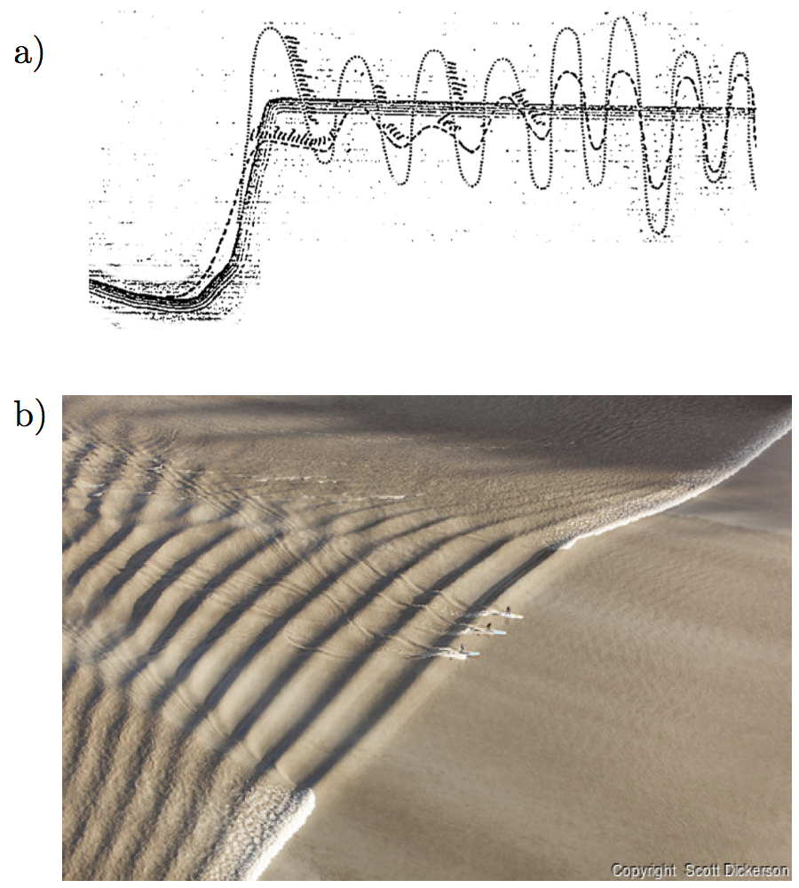
Figure 23: Undular bores. a) Measurements of a DSW generated by a hydraulic jump on Pont-aqueduc de Crau, Canal de Craponne, France in 1865 [21, 190]. b) Three standing paddle board riders on a river undular bore in Turnagain Arm, Alaska (copyright Scott Dickerson, 2013).

The dispersion relation of (4.42) for linear waves propagating on the background $\eta=\bar{\eta}$, $u=\bar{u}$ has the form

$$\omega_{\pm}(k;\bar{\eta},\bar{u})=k\bar{u}\pm\frac{k\bar{\eta}^{1/2}}{(1+\bar{\eta}^{2}k^{2}/3)^{1/2}}\,.$$ (4.43)

One can readily see that $\mathrm{sgn}\,[\partial_{kk}\omega_{+}]=-1$, implying the orientation $d=1$ for 2-DSWs. The solitary wave solutions of (4.42) are waves of elevation, hence the polarity $p=1$ of DSWs in terms of $\eta$, propagating on the background $\eta=\bar{\eta},u=\bar{u}$, and are characterized by the following speed-amplitude relation [192]

$$c_{s}(a;\bar{\eta},\bar{u})=\bar{u}+\sqrt{\bar{\eta}+a}.$$ (4.44)

The dispersionless limit of the Serre equations is the ideal shallow-water system. Thus the locus of faster, 2-DSWs connecting the left state $\eta=\eta_{-},\ u=u_{-}$ and the right state $\eta=\eta_{+},\ u=u_{+}$ is given by the dispersionless limit 2-wave curve:

$$u_{+}-2\eta_{+}^{1/2}=u_{-}-2\eta_{-}^{1/2}.$$ (4.45)

Without loss of generality, we assume $\eta_{+}=1$, $u_{+}=0$. Numerical solution of the Serre equations with the Riemann data satisfying (4.45) is shown in Fig. 24 and indeed exhibits a single, 2-DSW with $d=1$, $p=1$.

Incorporating the DSW locus (4.45) into the linear dispersion relation (4.43) by imposing the constraint $\bar{u}(\bar{\eta})=2(\bar{\eta}^{1/2}-1)$, we obtain for the frequency of the fast linear waves

$$\begin{split}\Omega(k,\bar{\eta})=\omega_{+}(k;\bar{\eta},\bar{u}(\bar{\eta}))\\ =2k(\bar{\eta}^{1/2}-1)+\frac{k\bar{\eta}^{1/2}}{(1+\bar{\eta}^{2}k^{2}/3)^{1/2}}\,.\end{split}$$ (4.46)

The second ingredient for DSW fitting analysis is the simple 2-wave’s characteristic speed for the dispersionless limit equations of $\bar{\eta},\bar{u}$,

$$V(\bar{\eta})=\bar{u}(\bar{\eta})+\bar{\eta}^{1/2}=3\bar{\eta}^{1/2}-2.$$ (4.47)

Then the characteristic ODEs (4.33), (4.34) for the trailing and leading edge become

$$\frac{dk}{d\bar{\eta}}=\frac{\partial\Omega/\partial\bar{\eta}}{V(\bar{\eta})-\partial\Omega/\partial k}\,,\qquad k(1)=0\,,$$ (4.48)

$$\frac{d\tilde{k}}{d\bar{\eta}}=\frac{\partial\tilde{\Omega}/\partial\bar{\eta}}{V(\bar{\eta})-\partial\tilde{\Omega}/\partial\tilde{k}}\,,\qquad\tilde{k}(\eta_{-})=0\,,$$ (4.49)

where $\tilde{\Omega}(\tilde{k},\bar{\eta})=-i\Omega(i\tilde{k},\bar{\eta})$. Given solutions of (4.48), (4.49), the velocities of the trailing and leading edges are found as

$$s_{-}=\frac{\partial\Omega}{\partial k}(k_{-},\eta_{-})\,,\qquad s_{+}=\frac{\Omega(\tilde{k}_{+},1)}{\tilde{k}_{+}}\,,$$ (4.50)

where $k_{-}=k(\eta_{-})$ and $\tilde{k}_{+}=\tilde{k}(1)$.

Equations (4.48), (4.49) assume a separable form by introducing $\alpha=(1+k^{2}\bar{\eta}^{2}/3)^{-1/2}$ and $\tilde{\alpha}=(1-\tilde{k}^{2}\bar{\eta}^{2}/3)^{-1/2}$ instead of $k$ and $\tilde{k}$ respectively. Then (4.48) becomes

$$\frac{d\bar{\eta}}{\bar{\eta}}=\frac{2(1+\alpha+\alpha^{2})}{\alpha(1+\alpha)(\alpha-4)}d\alpha\,,\quad\alpha(1)=1\,.$$ (4.51)

Equation (4.51) is readily integrated to give

$$\bar{\eta}=\frac{1}{\sqrt{\alpha}}\left(\frac{4-\alpha}{3}\right)^{21/10}\left(\frac{1+\alpha}{2}\right)^{2/5}\,.$$ (4.52)

Next, using (4.50), (4.46) we obtain an implicit expression for the trailing edge $s_{-}$ in terms of the total depth ratio across the DSW $\Delta=\eta_{-}/\eta_{+}=\eta_{-}$:

$$\begin{split}\sqrt{\beta}\Delta-\left(\frac{4-\beta}{3}\right)^{21/10}\left(\frac{1+\beta}{2}\right)^{2/5}=0\,,\\ \hbox{where}\ \ \beta=\left(\frac{2+s_{-}}{\sqrt{\Delta}}-2\right)^{1/3}\,.\end{split}$$ (4.53)

Similarly, integrating the ODE (4.49) and using the definition of the leading edge velocity (4.50), we obtain an implicit equation for $s_{+}$,

$$\frac{\Delta}{\sqrt{s_{+}}}-\left(\frac{3}{4-s_{+}}\right)^{21/10}\left(\frac{2}{1+s_{+}}\right)^{2/5}=0\,.$$ (4.54)

Figure 24: The numerical solution of the Serre equations (4.42) for smoothed Riemann initial data producing a single 2-DSW at $t=250$. Initial Riemann data: $\eta_{-}=\Delta=1.2,\ \eta_{+}=1,u_{-}=2(\sqrt{\eta_{-}}-1),\ u_{+}=0$. Reprinted with permission from [192], copyright 2006, American Institute of Physics.

Figure 25: The leading $s_{+}$ (upper curve) and trailing $s_{-}$ (lower curve) edge speeds vs the depth ratio $\Delta$ across the 2-DSW of the Serre equations. Dashed line: modulation solution (4.53), (4.54); Diamonds: values of $s_{-}$ extracted from the full numerical solution; Dotted line: the KdV DSW boundaries. Reprinted with permission from [192], copyright 2006, American Institute of Physics.

From the expression (4.44) relating the speed and the amplitude of the soliton, and the identification of the leading edge speed with the soliton speed $s_{+}=c_{s}(a_{+};1,0)$, we derive the equation for the amplitude $a_{+}$ of the leading solitary wave for the free surface elevation,

$$\begin{split}\frac{\Delta}{(a_{+}+1)^{1/4}}-\left(\frac{3}{4-\sqrt{a_{+}+1}}\right)^{21/10}\\ \times\left(\frac{2}{1+\sqrt{a_{+}+1}}\right)^{2/5}=0\,.\end{split}$$ (4.55)

Expansion of (4.55) for small jumps $\delta=\Delta-1$ yields $a^{+}=2\delta+O(\delta^{2})$ which agrees to leading order with the KdV result eq. (3.13).

Now we need to check the admissibility conditions. The causality inequalities (4.29) assume the form

$$\begin{split}\Delta^{1/2}-2<s_{-}<3\Delta^{1/2}-2\,,\\ s_{+}>1\,,\quad s_{+}>s_{-}\,,\end{split}$$ (4.56)

and can be shown to be satisfied for all $\Delta$ [192]. However, the monotonicity condition for $s_{-}(\Delta)$ (eq. (4.35)) can be shown to exhibit breakdown at $\Delta=\Delta_{c}\approx 1.43$. This is the indication of linear degeneracy of the modulation system occuring for $\Delta>\Delta_{c}$ and thus, inapplicability of the simple-wave integral curve for such jumps. The comparison of the modulation solution and numerical curves for the DSW speeds as function of $\Delta$ is shown in Fig. 25 and demonstrates excellent agreement for a broad range of $\Delta$. One can see that the analytical and numerical curves for the leading edge start to diverge for $\Delta>\Delta_{c}$ but, surprisingly, the trailing edge curve still agrees with numerics even for values of $\Delta$ well beyond $\Delta_{c}$ where, formally, the simple wave DSW fitting is not applicable. Also shown in Fig. 25 are appropriately scaled speeds of the KdV DSW. One can see that for small jumps the KdV and Serre DSW speeds agree quite well but quickly start to diverge as $\Delta$ increases.

An interesting observation made in [192] is that for large values of $\Delta$, the DSW apparently satisfies the classical Rankine-Hugoniot relations rather than the DSW locus (4.45). A similar observation has been made for DSWs in the photo-refractive NLS equation [198] where simple-wave DSW theory also experiences linear degeneracy breakdown, although the nonmonotonicity is now exhibited by the leading edge due to a different dispersion sign [57], see Section 4.2.3 below. This apparent effect of the Rankine-Hugoniot locus appearing in conservative dispersive systems still requires explanation.

Concluding this section, we note that the DSW fitting method can be extended to estimate the number of solitary waves and their distribution over amplitude in solitary wave trains developing from large-scale, decaying initial profiles $\eta_{0}(x)$, $u_{0}(x)$ satisfying the simple-wave condition $u_{0}(x)-2\sqrt{\eta_{0}(x)}=const$ for fast waves [199]. The results of [199] are “non-integrable” analogues of the Karpman results [124, 66] for the KdV equation based on semi-classical Bohr-Sommerfeld quantization, see Section 3.2.4.

4.2.3 DSWs in nonlinear optics

Intense laser beam propagation through defocusing (normal dispersion) optical media can lead to the generation of DSWs. Observations in optical fibers [8, 200, 16] and in spatial optics [10, 11, 13, 14, 15, 201] support the interpretation of light as a dispersive hydrodynamic medium.

The dispersive hydrodynamics of light can be modeled with the gNLS equation (recall (1.4))

$$i\psi_{z}+\frac{1}{2}\nabla^{2}\psi-f(|\psi|^{2})\psi=0,$$ (4.57)

where $z$ is the propagation direction, playing the role of time, and the Laplacian term represents either diffraction in the transverse direction $\nabla^{2}=\partial_{xx}+\partial_{yy}$ for spatial optics or temporal dispersion $\nabla^{2}=\partial_{tt}$ in fibers. The nonlinearity $f$, assumed positive and an increasing function of its argument, is due to an intensity dependent refractive index. The simplest example is the Kerr electrooptic effect where $f(\rho)=\rho$ [170], and we obtain the integrable, defocusing NLS equation (2.110), $\sigma=1$ assuming one transverse direction. This form is often used to model fibers. Another example is photorefractive, spatial media where the nonlinearity takes the form [170]

$$f(\rho)=\frac{\rho}{1+\gamma\rho},\quad\gamma>0.$$ (4.58)

Two-dimensional DSWs imaged from a photorefractive crystal are shown in Fig. 1c,d and two counter-propagating one-dimensional DSWs are shown in Fig. 26 [10]. Other examples include nonlocal, e.g., thermal [13] or nematic liquid crystal [202], media where $f$ is found by inverting an elliptic operator, an additional source of dispersion. We will focus on the one-dimensional case, taking $\nabla^{2}=\partial_{xx}$ for simplicity.

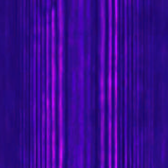
Figure 26: Image of the output face of a defocusing, photorefractive crystal resulting from a pulse at the input face. Two counter-propagating, one-dimensional DSWs resulting from wavebreaking. Reprinted by permission from Macmillan Publishers Ltd: Nature Physics [10], copyright 2007.

The hydrodynamic form for the gNLS equation is given in eqs. (1.3) and (1.6) via the mapping of the complex wavefunction $\psi\to\sqrt{\rho}\exp(i\int u\,\mathrm{d}x)$ (eq. (1.5)) and we take $t\to z$. DSWs for gNLS were constructed utilizing the DSW fitting method for photorefractive nonlinearity (4.58) in [198] and for general nonlinearities in [57]. In what follows, we first identify some properties of the gNLS equation and then apply the DSW fitting method to the photorefractive nonlinearity case.

We verify the requisite ingredients to apply Whitham theory. The dispersion relation for the hydrodynamic form of the gNLS equation is

$$\begin{split}\omega_{\pm}(k,\rho_{0},u_{0})&=u_{0}k\pm k\sqrt{c_{0}^{2}+k^{2}/4}\\ &\sim V_{\pm}(\rho_{0},u_{0})k\,\pm\,\frac{1}{8c_{0}}k^{3}+O(k^{5}),\end{split}$$

where

$$\begin{split}V_{\pm}(\rho_{0},u_{0})&=u_{0}\pm c_{0},\\ c_{0}&=\sqrt{\rho_{0}f^{\prime}(\rho_{0})},\end{split}$$

so that the dispersion sign is positive $\mathrm{sgn}\,\partial_{kk}\omega_{+}>0$ for 2-DSWs. This suggests that the 2-DSW will have orientation $d=-1$. For photorefractive nonlinearity (4.58), we obtain the long wavelength speed of sound

$$c(\rho)=\frac{\sqrt{\rho}}{1+\gamma\rho}.$$

The dispersionless limit is strictly hyperbolic and genuinely nonlinear so long as $(\rho f^{\prime}(\rho))^{\prime}>0$. This enforces the restriction $\gamma\rho<1$ in the case of photorefractive nonlinearity. The gNLS equation admits the local energy conservation law [104]

$$\begin{split}&\mathcal{E}=\frac{1}{2}\rho u^{2}+\frac{\rho_{x}^{2}}{8\rho}+\int_{0}^{\rho}f(\tilde{\rho})\,\mathrm{d}\tilde{\rho},\\ &\mathcal{E}_{z}+\big{(}u(\mathcal{E}+P(\rho))\big{)}_{x}=\frac{1}{4}\left(u\rho_{xx}-\frac{\rho_{x}(\rho u)_{x}}{\rho}\right)_{x}.\end{split}$$

A traveling wave solution $\rho(x,z)=\tilde{\rho}(x-Vz)$, $u(x,z)=\tilde{u}(x-Vz)$ satisfies (dropping tildes)

$$\begin{split}u&=V+\frac{A}{\rho}\\ (\rho^{\prime})^{2}&=8\rho\int_{0}^{\rho}f(\tilde{\rho})\,\mathrm{d}\tilde{\rho}+B\rho^{2}+C\rho-4A^{2}\\ &\equiv G(\rho),\end{split}$$

where $A$, $B$, and $C$ are integration constants. For photorefractive nonlinearity (4.58),

$$G(\rho)=-\frac{8}{\gamma^{2}}\rho\ln(1+\gamma\rho)+B\rho^{2}+C\rho-4A^{2},$$

where we have absorbed an integration constant by redefining $B$. We assume the existence of three real, ordered roots $G(b_{i})=0$, $i=1,2,3$. Since $G(0)=-4A^{2}<0$, the density of the periodic solution oscillates between $0<b_{1}$ and $b_{2}$. The three parameters $A$, $B$, and $C$ can be related to the three roots. The roots $\{b_{i}\}_{i=1}^{3}$ and $V$ can further be related to the physical modulation variables $\overline{\rho}$, $\overline{u}$, $k$, and $\tilde{k}$ per the standard approach described in Sec. 4.1. Finally, we can identify the soliton amplitude-speed relation in the limit $b_{2}\to b_{3}$

$$\begin{split}(V-\overline{u})^{2}=&\frac{2\rho_{\rm min}f(\overline{\rho})}{\overline{\rho}-\rho_{\rm min}}\\ &\qquad-\frac{2\rho_{\rm min}}{(\overline{\rho}-\rho_{\rm min})^{2}}\int_{\rho_{\rm min}}^{\overline{\rho}}f(\tilde{\rho})\,\mathrm{d}\tilde{\rho},\end{split}$$ (4.59)

where $\rho_{\rm min}\equiv\min_{\xi\in\mathbb{R}}\rho(\xi)$ is the minimum of the “dark” or depression soliton implying the DSW polarity $p=-1$.

The final ingredients we need to implement DSW fitting are the Riemann invariants of the dispersionless limit (4.21)

$$r_{\pm}=u\pm\int\sqrt{\frac{f^{\prime}(\rho)}{\rho}}\,\mathrm{d}\rho.$$

For photorefractive nonlinearity, we have

$$r_{\pm}=u\pm\frac{2}{\sqrt{\gamma}}\mathrm{arctan}\,(\sqrt{\gamma\rho}).$$

We now focus upon the case of photorefractive nonlinearity as in [198]. We introduce the locus of left states $(\overline{\rho},\overline{u})$ that can be connected to the right state $(\rho_{\rm r},u_{\rm r})$ by a 2-DSW (4.28)

$$\overline{u}(\overline{\rho})=u_{\rm r}+\frac{2}{\sqrt{\gamma}}\mathrm{arctan}\left(\frac{\sqrt{\gamma\overline{\rho}}-\sqrt{\gamma\rho_{\rm r}}}{1+\gamma\sqrt{\overline{\rho}\rho_{\rm r}}}\right),\quad\overline{\rho}>\rho_{\rm r}.$$ (4.60)

This is the local relation (4.32) that holds for a simple wave solution along the exact reductions of the Whitham equations.

Because the DSW orientation $d=-1$, the DSW leading edge speed $s_{\rm r}$ is associated with the harmonic limit and the simple wave ODE (4.33) subject to the zero wavenumber boundary condition at the left edge $k(\rho_{\rm l})=0$. This ODE for $k(\overline{\rho})$ is somewhat complicated and can be simplified by the transformation

$$\alpha(\overline{\rho})=\frac{\omega_{+}-\overline{u}(\overline{\rho})k}{c(\overline{\rho})k}=\sqrt{1+\frac{k^{2}(1+\gamma\overline{\rho})^{2}}{4\overline{\rho}}},$$ (4.61)

to a scaled phase velocity. Then $\alpha(\overline{\rho})$ satisfies

$$\begin{split}\frac{\,\mathrm{d}\alpha}{\,\mathrm{d}\overline{\rho}}&=-\frac{(1+\alpha)\left(1+3\gamma\overline{\rho}+2\alpha(1-\gamma\overline{\rho})\right)}{2\overline{\rho}(1+\gamma\overline{\rho})(1+2\alpha)},\end{split}$$ (4.62)

subject to the initial condition

$$\alpha(\rho_{\rm l})=1.$$

Integration of (4.62) results in $\alpha_{\rm r}=\alpha(\rho_{\rm r})$, which via (4.61) yields $k_{\rm r}$. The leading edge speed is therefore the group velocity $s_{\rm r}=\partial_{k}\omega_{+}(\rho_{\rm r},u_{\rm r},k_{\rm r})$.

A similar analysis at the soliton, trailing edge can be performed in order to determine the trailing edge speed $s_{\rm l}$. The simple wave ODE (4.34), subject now to $\tilde{k}(\rho_{\rm r})=0$, can again be simplified by the transformation

$$\tilde{\alpha}(\overline{\rho})=\frac{\tilde{\omega}_{+}-\overline{u}(\overline{\rho})\tilde{k}}{c(\overline{\rho})\tilde{k}}=\sqrt{1-\frac{\tilde{k}^{2}(1+\gamma\overline{\rho})^{2}}{4\overline{\rho}}},$$ (4.63)

to a scaled phase velocity. Then $\tilde{\alpha}(\overline{\rho})$ satisfies the same equation (4.62) with $\alpha\to\tilde{\alpha}$ subject to the boundary condition at the leading edge

$$\tilde{\alpha}(\rho_{\rm r})=1.$$ (4.64)

Integration of (4.62) with $\alpha\to\tilde{\alpha}$ and (4.64) results in $\tilde{\alpha}_{\rm l}=\tilde{\alpha}(\rho_{\rm l})$, which via (4.63) yields $\tilde{k}_{\rm l}$. The trailing edge speed is therefore the phase velocity $s_{\rm l}=\tilde{\omega}_{+}(\rho_{\rm l},u_{\rm l},\tilde{k}_{\rm l})/\tilde{k}_{\rm l}$.

Here we reach an obstacle that sometimes arises in applications. The simple wave ODE (4.62) at both the leading and trailing edges cannot be integrated analytically. Several options are available. Recalling that photorefractive nonlinearity (4.58) can be considered a perturbation to the integrable NLS equation when $0<\gamma\ll 1$, one could appeal to an asymptotic analysis of (4.62). Alternatively, one can numerically integrate (4.62) to obtain predictions for $s_{\pm}$. Both of these strategies were carried out in [198].

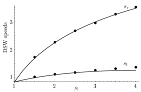
Figure 27: DSW leading $s_{\rm r}$ and trailing $s_{\rm l}$ speeds as a function of the left density $\rho_{\rm l}$ with $u_{\rm l}=\overline{u}(\rho_{\rm l})$ (eq. (4.60)), $\rho_{\rm r}=1$, $u_{\rm r}=0$, and $\gamma=0.2$. Reprinted figure with permission from [198] copyright 2007 by the American Physical Society.

Figure 27 depicts the DSW leading and trailing edge speeds for a 2-DSW computed from the DSW fitting procedure (solid curves) and from direct numerical simulation of the gNLS equation (4.57) with photorefractive nonlinearity (4.58) [198]. The DSW fitting procedure yields excellent agreement across a range of density jumps.

An example DSW resulting from the shock tube problem with $u_{\rm l}=u_{\rm r}=0$ and $\rho_{\rm l}>\rho_{\rm r}$ is shown in Fig. 28a. The dispersive shock tube results in the generation of a 1-rarefaction propagating upstream and a 2-DSW downstream.

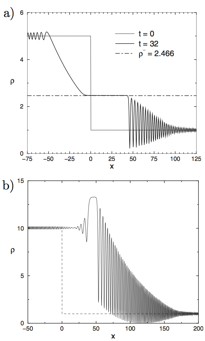
Figure 28: Numerically computed DSWs for the gNLS equation with photorefractive nonlinearity. a) Shock tube problem with $\rho_{\rm l}=5$, $\rho_{\rm r}=1$, $u_{\rm l}=u_{\rm r}=0$, and $\gamma=0.1$. b) 2-DSW resulting from $\rho_{\rm l}=10$, $\rho_{\rm r}=1$, $u_{\rm l}=\overline{u}(10)$ (eq. (4.60)), $u_{\rm r}=0$, $\gamma=0.2$. Reprinted figures with permission from [198] copyright 2007 by the American Physical Society.

It was observed in [198] that for 2-DSW density jumps $\rho_{\rm l}/\rho_{\rm r}\gtrsim 4$, the DSW structure is altered and there is a significant discrepancy between the prediction for $s_{\rm l}$ and the observed soliton edge as we can begin to see in Fig. 27. An example profile is shown in Fig. 28b. We see that $\gamma\rho$ significantly exceeds unity ($\gamma=0.2$ in Fig. 28b), therefore the dispersionless system loses genuine nonlinearity. As described in Sec. 5, new wave structures are possible when scalar dispersive hydrodynamics exhibit a non-convex flux. The linearly degenerate point $\gamma\rho=1$ is the hyperbolic system analogue of an inflection point in the scalar flux.

Although the simple wave ODE (4.62) is complex, additional analysis is still available [198, 57]. For example, equating the soliton amplitude-speed relation (4.59) to the trailing edge speed $V=s_{\rm l}$, one can determine the DSW trailing edge amplitude. Moreover, one can see directly from eq. (4.59) the possibility that $\rho_{\rm min}=0$, i.e., the existence of a vacuum point. An internal vacuum point is visible in Fig. 28b. There are also admissibility conditions (4.29) to check. Finally, an extremum in either of the DSW speeds as a function of $\rho_{\rm l}$ or $\rho_{\rm r}$ is associated with a breakdown of the simple wave assumption [57]. An extremum in $s_{\rm l}$ for the 2-DSW constructed here was observed in [198] when $\rho_{\rm l}\approx 4$, $\rho_{\rm r}=1$, and $\gamma=0.2$. This critical jump height was exceeded for the simulation in Fig. 28b.

In summary, the DSW fitting method applied to non-integrable dispersive hydrodynamic problems yields practical results that agree with numerical simulations across a wide range of parameters. The break down of the method can be identified by structural properties of the zero amplitude or zero wavenumber reductions of the Whitham modulation equations [57].

5 Non-classical DSWs

The DSW theory described in the previous sections can be viewed as the dispersive-hydrodynamic counterpart of classical viscous shock theory. The admissibility criteria for such viscous shocks include the causality conditions, termed Lax entropy conditions [41]. An analogous set of causality conditions has been introduced for DSWs (see Sec. 4.1). In classical shock theory, the notion of a Lax shock is closely related to convexity of the flux of the underlying hyperbolic conservation law $u_{t}+f(u)_{x}=0$: in a system with convex or concave flux, i.e., $f^{\prime\prime}(u)\neq 0$ for a scalar equation, all admissible shock waves are Lax shocks.

When the flux $f(u)$ is non-convex, i.e. $f^{\prime\prime}(u)=0$ at some point within the range of $u$, new wave features emerge in hyperbolic shock theory including composite wave solutions and undercompressive shocks that do not satisfy the Lax entropy condition [203]. One of the standard approaches to shock admissibility analysis involves regularization of the equation by higher order terms that are dissipative and dispersive, representing more of the physics than is contained in the hyperbolic conservation law alone. For scalar conservation laws with convex flux, the fundamental model describing a diffusive-dispersive regularization is the KdV-Burger’s equation (1.7) considered in Sec. 1.2. For non-convex conservation laws, such a model is the modified KdV-Burger’s (mKdVB) equation,

$$u_{t}+(u^{3})_{x}=\nu u_{xx}+\mu u_{xxx},\quad\nu\geq 0,\ \ \mu\neq 0.$$ (5.1)

The remarkable feature of the mKdVB equation is that it exhibits, for $\mu>0$, traveling waves called undercompressive shocks because the corresponding limiting ($\nu/\sqrt{|\mu|}\to 0$) shock wave

$$u(x,t)=\left\{\begin{array}[]{ll}u_{-},&x<st\\[6.0pt] u_{+},&x>st\end{array}\right.$$ (5.2)

is subsonic both ahead of and behind the wave:

$$|s|<V(u_{\pm})=3u^{2}_{\pm},$$ (5.3)

where $V$ is the characteristic velocity or sound speed.

Shock wave theory for the mKdVB equation was constructed in [204] by analyzing traveling wave solutions, where it was shown that undercompressive shocks appear only for $\mu>0$. When $\mu<0$ there are no undercompressive shocks but there are shock-rarefaction complexes exhibiting contact shocks propagating with the sound speed.

What would be the counterparts of these “non-classical” shock phenomena in the inviscid case when $\nu=0$ so that eq. (5.1) becomes the conservative mKdV equation? Or, putting it the other way around, what is the effect of a non-convex hyperbolic flux on the solutions of dispersive Riemann problems, and, in particular, on the modulation theory of DSWs? This question is not only of significant mathematical interest but is also important for applications, such as oceanography and nonlinear optics where dispersive-hydrodynamic systems with nonconvex hyperbolic flux are quite common. A prominent model is the Gardner equation, the combined KdV-mKdV equation, which is the standard model for internal waves in stratified fluids [205] but also arises in plasma physics [206] and BEC dynamics [207]. The Gardner equation is mathematically equivalent to the mKdV equation, however, the transformation between mKdV and Gardner involves a change of boundary conditions at infinity, which is not always physically acceptable so the use of Gardner, rather than mKdV, can be essential for applications. The fully nonlinear bi-directional counterpart of the Gardner equation, the Miyata-Choi-Camassa (MCC) system [208] is a two-layer generalization of the Serre system (4.42). The dispersionless limit of the MCC system is the two-layer ideal shallow water system exhibiting non-genuine nonlinearity [209]. Other important non-convex dispersive hydrodynamic models include the cubic-quintic NLS equation [212] describing, in particular, the evolution of the complex wavefunction $\psi$ of a Bose-Einstein condensate with two- and three-body interactions, and the so-called derivative NLS equation for nonlinear Alfven waves in dispersive magnetohydrodynamics [213].

Analysis of the traveling wave solutions of the mKdV (or Gardner) equation [214, 40] shows that, along with familiar KdV type cnoidal waves and solitons of both polarities, due to the symmetry $u\to-u$ of the mKdV equation, two new types of solutions emerge: for $\mu>0$ these new solutions are termed kinks or anti-kinks while for $\mu<0$ there are nonlinear trigonometric solutions. Kinks are smooth, propagating fronts connecting conjugate states $u\to u_{\pm}$, $u_{-}=-u_{+}$ as $x\to\pm\infty$ and propagate with the classical shock speed $s=u_{+}^{2}$ of the hyperbolic conservation law $u_{t}+(u^{3})_{x}=0$. The kink solution of the mKdV equation with $\mu>0$ is described by the formula

$$\begin{split}u&=u_{+}\tanh[u_{+}\eta]\,,\quad\eta=\frac{x-u_{+}^{2}t}{\sqrt{2\mu}}.\end{split}$$ (5.4)

The kink speed satisfies (5.3) and thus the kink represents an undercompressive DSW, the direct counterpart of the undercompressive shock wave of the mKdVB equation. Having the restricted locus $u_{+}+u_{-}=0$, kinks are usually generated in Riemann problems as part of a double wave structure, the other part being either a “classical”, KdV-type DSW or a rarefaction wave (see Fig. 29). Depending on the initial step parameters, DSWs of both polarities can be generated (separately or in combinations with kinks/anti-kinks).

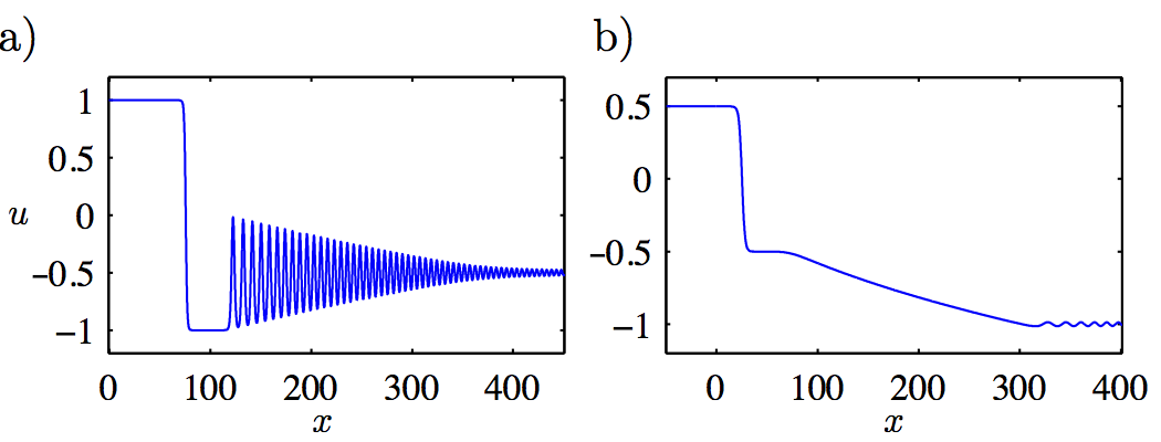
Figure 29: Numerical solutions of the mKdV equation (5.1) ($\nu=0$, $\mu=1>0$) with step-like initial data. a) kink-DSW; b) kink-rarefaction.

The mKdV equation with $\mu<0$ supports another non-classical family of traveling wave solutions, which are described in terms of trigonometric functions with no linearization involved. These trigonometric solutions are the “carrier waves” for contact DSWs (CDSWs), some of which do not have counterparts in the diffusive-dispersive theory of the mKdVB equation [40]. CDSWs, similar to kinks, have the restricted locus $u_{+}+u_{-}=0$ and so usually are generated in combination with a rarefaction (see Fig. 30a) or are realized only partially, forming part of a compound wave — the CDSW$|$DSW complex (Fig. 30b). When fully realized, a CDSW exhibits an algebraic soliton at its leading edge. CDSWs always exhibit a “Bordeaux glass” type envelope.

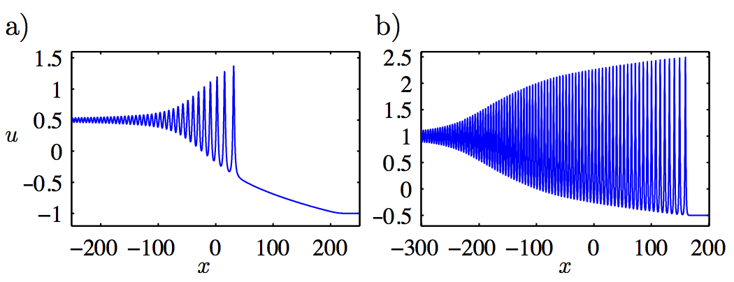
Figure 30: Numerical solutions of the mKdV equation (5.1) ($\nu=0$, $\mu=-1<0$) with step-like initial data. a) CDSW-rarefaction; b) CDSW$|$DSW.

The modulation system for the mKdV equation was first derived in an analogous fashion to Whitham’s derivation of the KdV modulation system [79] (see Sec. 2.2.2) by averaging the first three mKdV conservation laws. It transpired later [215, 216], and more generally in [214] using a reduced version of finite-gap spectral theory [54], that the modulation system for the mKdV equation with $\mu>0$ can be mapped onto the KdV modulation system (2.51). The mapping can be viewed as the modulation theory counterpart of the Miura transform [80]. It was also shown in [79] that the modulation system for the mKdV equation with $\mu<0$ can be elliptic, which is the signature of nonlinear modulational instabilty. However, this unstable regime is not realized by solutions of the Riemann problem. Further, it was shown in [40] that within the hyperbolic region, the mKdV-Whitam system is neither genuinely nonlinear nor strictly hyperbolic, leading to the breakdown of the “classical” DSW admissibility conditions and the occurrence of solutions that cannot be realized in convex dispersive hydrodynamics. Other modulation systems exhibiting non-strict hyperbolicity and yielding novel dynamics not captured by classical DSW theory have been studied in [217] (the integrable fifth order KdV equation), [218] (the complex modified mKdV equation) and [219] (the Camassa-Holm equation).

The modulation solutions for DSWs in the mKdV equation with $\mu<0$ were first constructed in [220], where the new DSW type realized by a modulated nonlinear trigonometric solution was termed “sinusoidal undular bore”. The analogous DSWs for the Gardner equation were studied in [214]. Their nature as contact DSWs was realized in [40] by an analysis of the modulation solution’s characteristics. The composite CDSW-rarefaction exhibits a triple characteristic at the interface between the CDSW and rarefaction, similar to the properties of a contact shock.

Elements of DSW theory for the mKdV equation with $\mu>0$ appear in [221] in the context of collisionless plasma physics. The detailed description of kink or CDSW emergence in Riemann problem solutions of the Gardner equation was carried out in [214] for both signs of $\mu$. These Gardner equation results were applied to the resonant generation of internal undular bores in stratified fluid flows over topography [222] (see Sec. 8). The very recent paper [40] contains detailed analysis of the nontrivial connections between the Riemann problem classifications of the mKdVB and mKdV equations.

DSW theory for non-integrable systems whose dispersionless limit lacks genuine nonlinearity is only just emerging with few existing contributions. The identification of kinks in fully nonlinear, near-critical, two-layer flows with undercompressive shocks was made in [223]. The paper [209] uses the DSW fitting method to describe the dispersive dam break and lock exchange flows in the framework of the MCC system. The authors show that MCC lock exchange flows give rise to kink-DSW compound wave complexes, similar to those found in the Gardner and mKdV equations in [214, 40] (see Fig. 29). The occurrence of DSWs with different polarities related to non-convex dispersive hydrodynamics in some solutions of the Riemann problem for the cubic-quintic NLS equation has been reported in [212].

6 DSW interactions

DSWs are coherent, long-lived structures. It is therefore natural to consider their interaction properties. Fundamental shock interactions include an overtaking interaction with two co-propagating shocks and a head-on interaction with two counter-propagating shocks. Typical dynamics for these two interaction types when the hydrodynamics are dispersionless (e.g., for the dispersionless KdV or Hopf equation (3.2) and the dispersionless NLS or shallow water equations (2.113)) are shown in Figs. 31 and 32. The overtaking viscous shock interaction results in the eventual merger of the two shocks (speeds $s_{1}>s_{2}$) into a single shock (speed $s_{\rm m}$). For nonconvex flux, the shock speeds are guaranteed to be interleaved

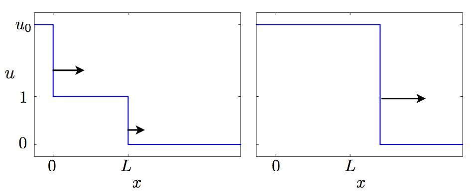
Figure 31: Schematic of an overtaking viscous shock interaction in uni-directional dispersionless hydrodynamics with time progressing to the right.

$$s_{2}<s_{\rm m}<s_{1}.$$ (6.1)

The symmetric head-on collision of two viscous shocks depicted in Fig. 32 shows that, post-interaction, two new shocks are generated with a larger density and propagate away from one another.

In this section, we consider the canonical overtaking DSW interaction in the context of uni-directional KdV dispersive hydrodynamics and the head-on DSW interaction for bi-directional NLS dispersive hydrodynamics. We conclude with interactions involving dispersively regularized rarefaction waves.

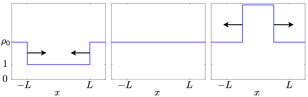
Figure 32: Schematic of the density for a head-on collision of two viscous shock waves in bi-directional dispersionless hydrodynamics with time progressing rightward.

6.1 Overtaking DSW interaction

We consider the KdV equation (2.33) with double-step initial conditions

$$u(x,0)=\begin{cases}u_{0}&x<0\\ 1&0<x<L\\ 0&L<x\end{cases},$$

where $u_{0}>1$. We assume that $L$ is large enough so that each DSW resulting from the initial two steps has sufficient distance to develop. Then the simple wave DSW analysis in Sec. 3.1 applies to the initial two DSWs. From eq. (3.12), the leftmost, faster DSW expands with speeds $s_{1,-}=-u_{0}+2$, $s_{1,+}=\frac{2}{3}u_{0}+\frac{1}{3}$ and the slower DSW propagates with speeds $s_{2,-}=-1$, $s_{2,+}=\frac{2}{3}$. If we simply assume, by motivation from the viscous case, that the two DSWs merge into a single DSW connecting $u=0$ and $u=u_{0}$, then its speeds are $s_{\textrm{m},-}=-u_{0}$ and $s_{\textrm{m},+}=\frac{2}{3}u_{0}$. This would imply that the soliton edge DSW speeds are interleaved

$$s_{2,+}<s_{\textrm{m},+}<s_{1,+},$$ (6.2)

as in the viscous shock case (6.1).

In fact, it has been shown using IST with matched asymptotic expansions [109] and the rigorous IST Riemann-Hilbert problem approach [160] that a general class of initial data with boundary conditions $u\to u_{\pm}$ as $x\to\pm\infty$ and $u_{+}>u_{-}$ result in a single DSW, dispersive radiation, and possibly solitons for large $t$. Thus, multiple KdV DSWs will eventually merge into a single DSW. An example numerical solution of the KdV equation (3.14) with multi-step initial data is shown in Fig. 33 [109].

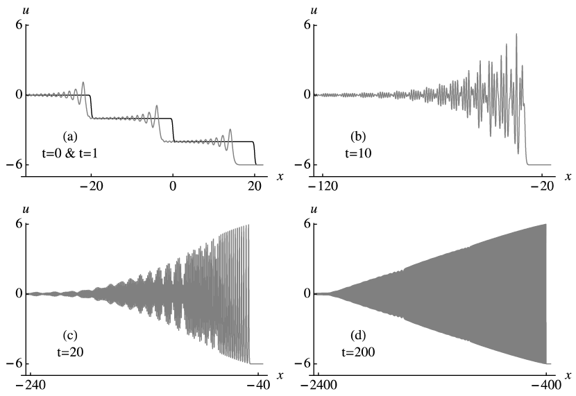
Figure 33: Numerical solution of the KdV equation (3.14) with $\varepsilon^{2}=0.1$ for multi-step initial data. The dynamics display a multiphase interaction region and the effective merger into a one-phase DSW after long time. Reprinted from [109] with permission from Elsevier.

Modulation theory provides additional information about the dynamics of step-like initial data [161]. Recall that a single DSW is described by KdV-Whitham modulations of a one-phase wave. When two DSWs collide, the one-phase equations exhibit a singularity and there is an increase in the number of phases required to describe the modulation solution. The resultant DSW interaction region is described by two-phase modulations, and can be viewed as the nonlinear superposition of two one-phase objects. The multiphase interaction region is eventually extinguished in long time, leaving just one-phase modulations (a single DSW). A rigorous examination of this was performed in [162].

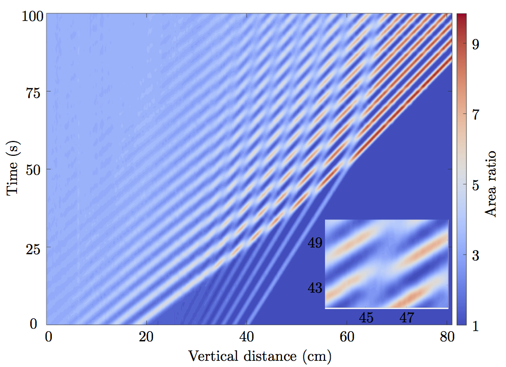
Figure 34: Contour plot in space-time depicting the normalized cross sectional area of an overtaking interaction experiment of viscous fluid conduit DSWs. A two-phase interaction region appears (inset) and is eventually extinguished. Figure provided with permission from [184].

The overtaking interaction of two DSWs is therefore quite similar to the same involving two viscous shock waves. The main difference is that, due to the nonzero spatial extent of DSWs, their interaction occurs over some time period, in contrast to the essentially instantaneous interaction of viscous shock waves. Using the generalized hodograph transform, the KdV modulation solution for the overtaking interaction of two DSWs was obtained in [121] and applied to the long-time evolution of shelves formed behind solitary wave propagation through an inhomogeneous medium. Numerical computations of an overtaking DSW interaction for both the KdV equation and the two-phase KdV-Whitham equations were performed in [236] (see also Fig. 37a).

Motivated by this KdV analysis, the merger of two co-propagating DSWs can be postulated a-priori, therefore making it possible to determine the macroscopic properties of an overtaking interaction of two DSWs in other model equations using the DSW fitting approach from Sec. 4.1. The overtaking interaction of two DSWs in uni-directional, dispersive hydrodynamics was observed in the viscous fluid conduit system (Sec. 4.2.1) [184] as shown in Fig. 34. The appearance and annihilation of a modulated two-phase interaction region is apparent. Moreover, the speed interleaving property (6.2) is also apparent and has been derived for conduit DSWs using the DSW fitting method of Sec. 4.2.1 [184].

6.2 Head-on DSW interaction

We now consider symmetric initial data for the defocusing NLS equation (2.110) ($\sigma=1$) leading to the generation of two counter-propagating NLS DSWs

$$\rho(x,0)=\begin{cases}\rho_{0}&|x|>L\\ 1&|x|<L\end{cases},\quad u(x,0)=\begin{cases}u_{0},&x<-L\\ 0&|x|<L\\ -u_{0}&x>L\end{cases},$$ (6.3)

where $\rho_{0}>1$ to guarantee DSW generation and $u_{0}=2(\sqrt{\rho_{0}}-1)$ lies on the 2-DSW locus (3.53). The result of numerical simulation of a smoothed version of this initial value problem is depicted in Fig. 35. Similar to the KdV case, the interaction of two NLS DSWs results in a two-phase interaction region. This two-phase behavior eventually subsides, leaving an unmodulated, zero phase region in its wake and two new DSWs propagating away from each other. These dynamics are, again, analogous to the dispersionless case of Fig. 32.

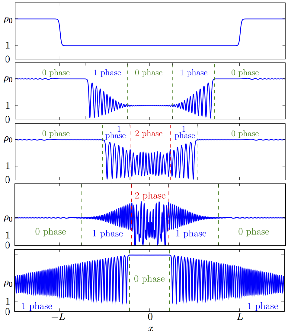
Figure 35: Density from the numerical solution of the NLS equation for a symmetric, head-on collision with time progressing downward. The number of phases required to describe each modulation region is noted. Figure adapted, with permission, from [210].

The head-on collision of two DSWs in the context of optical four-wave mixing was observed in [16]. Figure 36 shows the onset of the collision process.

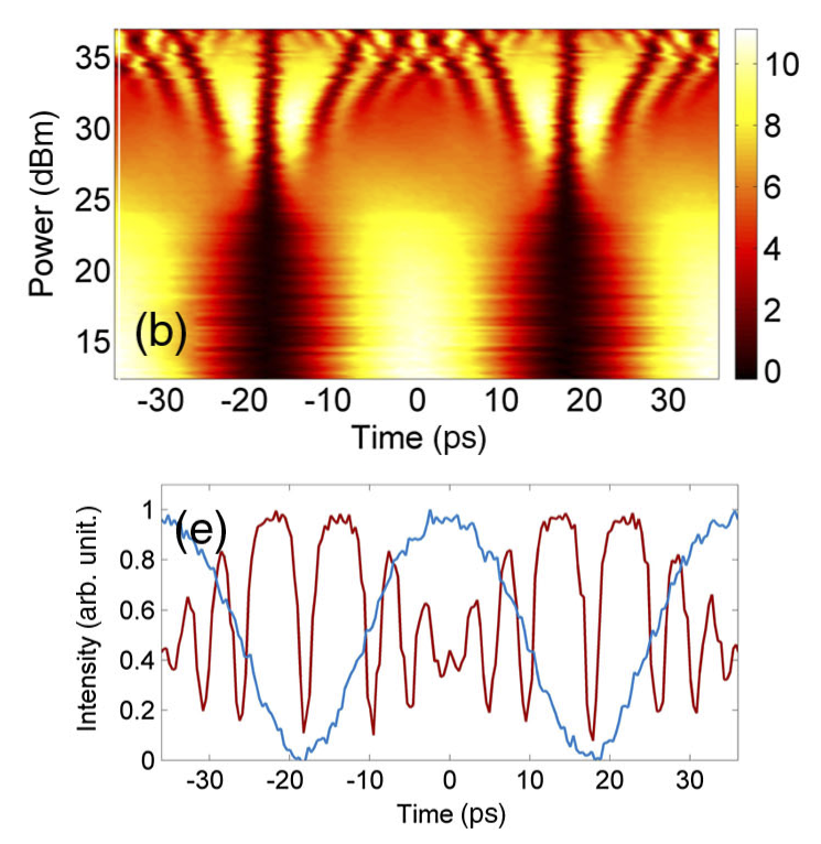
Figure 36: Head-on DSW collision observation in optical four-wave mixing. Top (b): Contour plot of output power (color) versus input power (vertical axis) and time (horizontal axis). Bottom (e) Output intensity (red) resulting from cosine input with power $P=34.6$ dBm (blue). Copyright [16], DOI:10.1103/PhysRevX.4.021022, Creative Commons 3.0, 2014.

As for the multi-step KdV DSW interaction problem, NLS modulation theory provides the means to identify the spontaneous creation and annihilation of phases in the modulation solution [135]. A convenient method to determine the dispersive regularization for piecewise constant initial conditions is initial data regularization [113, 114]. Degenerate initial conditions for the Whitham equations corresponding to a minimum number of phases in the modulation solution are chosen so that a global solution is obtained. The overlap of two Riemann invariants effectively nullifies the role of one phase in the modulation solution. As the modulation solution evolves, Riemann invariants may separate (or merge), giving rise to the appearance (or annihilation) of an additional phase in the solution. Using this method, it was shown in [114] that the long time evolution of piecewise constant initial data for NLS can be described by expanding zero-, one-, and two-phase regions but no higher phase regions. In [210], this method was utilized to determine the space-time boundaries for the number of phases required to describe the head-on and overtaking interaction of NLS DSWs. For example, dispersive regularization of the initial data (6.3) requires six Riemann invariants to guarantee a global solution of the NLS-Whitham equations. This implies that, at most, two phases will appear in the solution. As shown in Fig. 35 for the symmetric, head-on DSW collision, this two-phase region is extinguished in finite time. The overtaking interaction of two NLS DSWs was also found to result in a single, merged DSW.

We note that soliton-DSW interactions were also observed in [184] and shown to exhibit soliton absorption or soliton refraction, depending on the initial ordering of the soliton and DSW. The theory of DSW-soliton interactions has not been developed.

6.3 DSW and rarefaction wave interactions

At the level of hyperbolic, dispersionless equations, shocks are not the only weak solutions available. Rarefaction waves can also exist and here we briefly examine their interaction properties in the context of dispersive hydrodynamics.

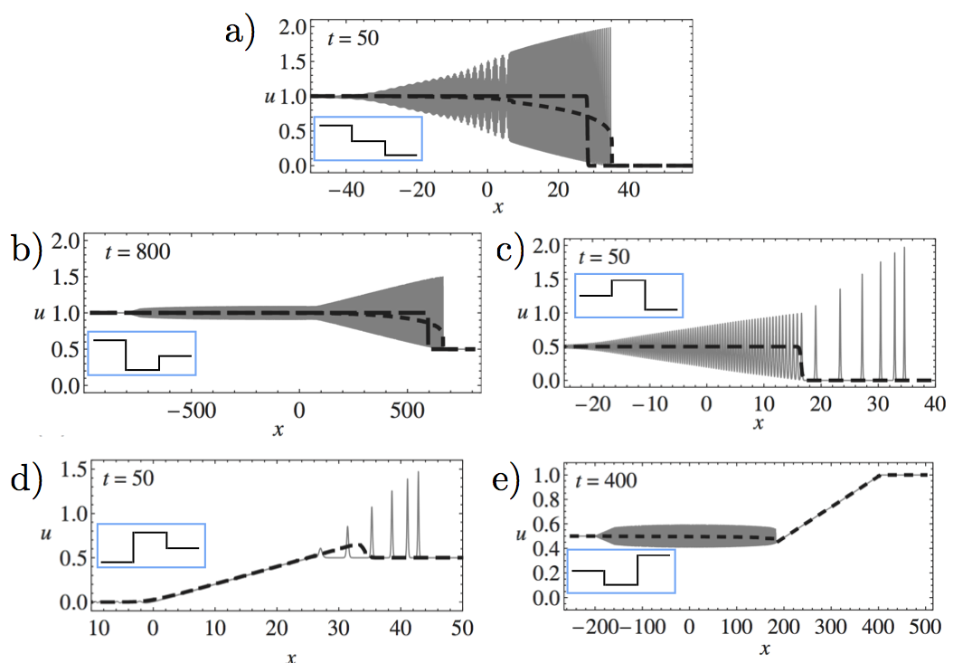
Figure 37: Numerical simulation (solid) and mean $\overline{u}$ from Whitham theory (short dash) for five of the six qualitatively distinct two-step initial conditions. The initial condition for each panel is shown as an inset. In a and b, the dissipative shock regularization of the Hopf equation is also shown (long dash). Figure adapted, with permission, from [236].

The six qualitatively distinct KdV wave interaction problems for two-step initial data were examined in [121, 236]. According to the classification in Fig. 9, a depression step gives rise to a DSW whereas an elevation step leads to a rarefaction wave. These six interaction problems can be conveniently visualized according to the relative magnitudes of $u$ adjacent to each step as follows:      ,      ,      ,      ,      ,      . Numerical solutions of the first five cases are depicted in Fig. 37. The final case      , not shown, results in a single rarefaction. Case       is the overtaking DSW interaction described in Sec. 6.1 (Fig. 37a). Case       results in a DSW on the left that eventually overtakes and absorbs a small rarefaction (Fig. 37b). The long tail is a remnant of the rarefaction-DSW interaction. The generation of a rarefaction on the left that interacts with a DSW, case      , leads to a single DSW and a finite number of solitons (Fig. 37c). The case       is qualitatively similar to the shoaling of an undular bore over a gentle slope and will be described in Sec. 7 (see Fig. 43). The large rarefaction in case       interacts with a DSW that eventually turns into a finite train of separated solitons (Fig. 37d). A small DSW cannot overtake the large rarefaction of case      , resulting in a single rarefaction with a small amplitude oscillatory tail (Fig. 37e).

In the NLS case, there are a number of qualitatively distinct solutions resulting from two-step initial data. Due to the large number, they have not all been classified. We consider two cases here: the refraction of a DSW by a rarefaction wave and the interaction of two degenerate rarefaction waves.

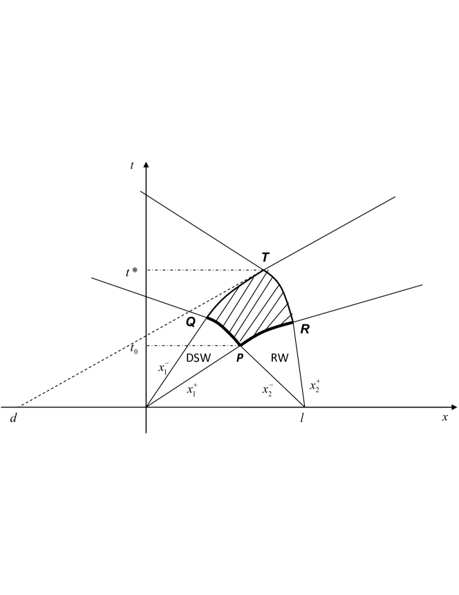
Figure 38: $x,t$-diagram of a 2-DSW interaction with a 1-rarefaction wave (RW). The interaction occurs within the region PQTR. The refraction shift $d$ of the DSW soliton edge quantifies the intensity of the interaction. Reprinted from [102] Copyright (2012), with permission from Elsevier.

The head-on interaction of a NLS DSW with a centered rarefaction wave has been considered in [102] as a dispersive counterpart of the classical gas dynamics problem of shock wave refraction (see, e.g., [141, 58]). When a one-dimensional viscous shock wave undergoes a head-on collision with a rarefaction wave, the parameters of the two waves alter so that the long-time output of such an interaction consists of a new pair of shock and rarefaction waves propagating in opposite directions. Since the shock wave speed undergoes a change from one constant value to another as a result of its propagation through the finite rarefaction region with varying density and velocity, the interaction diagram in the $x,t$ plane is naturally interpreted as shock wave refraction on the rarefaction wave. The $x,t$ diagram of the interaction between a 2-DSW and a 1-rarefaction wave is shown in Fig. 38. The interaction occurs within the region PQTR and is described by the classical hodograph solution of the NLS-Whitham equations in which only two Riemann invariants vary. As a result, the interaction dynamics are expressed in terms of the solution of a single EPD equation (2.98) in the plane of varying Riemann invariants. The intensity of the interaction is macroscopically quantified by the refraction shift $d$ of the DSW soliton edge.

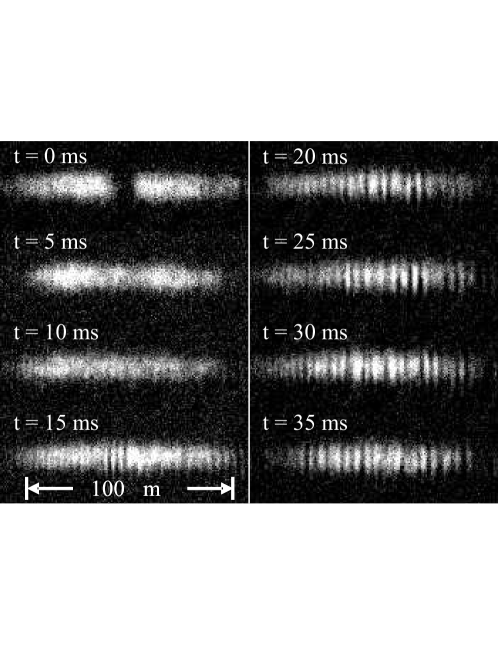
Figure 39: Density from a matter wave interference experiment in a Bose-Einstein condensate. Reprinted from [6] with permission from Elsevier.

The second type of interaction we consider is that of two degenerate rarefaction waves. As noted in Sec. 3.3.1, a sharp transition into the vacuum state $\rho=0$, will always result in a degenerate rarefaction wave. Much like the interaction of two DSWs generates two-phase modulations, the collision of two counter-propagating, degenerate rarefaction waves leads to one phase modulations. This model problem has significance in BEC when two initially separated clouds are allowed to merge together. The result is matter wave interference, a macroscopic realization of the quantum, wave nature of matter [211]. An experimental realization of this is shown in Fig. 39 [6]. The modulation solution corresponding to the interaction of two degenerate rarefaction waves is shown in Fig. 40. Nonlinear matter wave interference can be interpreted as the generation of two back-to-back DSWs, analogous to the dispersionless, hyperbolic case, also shown in Fig. 40. Note that the experiment pictured in Fig. 39 was also performed with weaker transverse confinement, giving rise to fully three-dimensional dynamics [5].

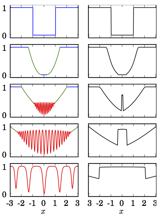
Figure 40: Density for degenerate rarefaction wave interaction in NLS (left) and dispersionless NLS (right) with time progressing downward. The NLS solution was constructed using Whitham theory [6]. Figure adapted from [6] with author permission.

In concluding this section, we note that the similarity between shock and rarefaction interactions for both dispersive and dissipative regularization of conservation laws is quite striking. The principle differences include the generation of finite time interaction regions and, possibly, solitons for the dispersive case.

7 DSWs in perturbed systems

All examples of DSWs considered so far have been described by solutions of constant coefficient, dispersive-hydrodynamic equations without perturbative and/or forcing terms. However, the presence of small perturbations in the system reflecting, e.g., the medium’s inhomogeneity or weak dissipation can strongly impact DSW dynamics. A fluid mechanics example of particular applied interest is the propagation of a shallow water DSW (surface or internal undular bore) over slowly varying bottom topography, termed shoaling. This example is of broader significance in the context of DSW propagation in weakly inhomogeneous media. We note that shoaling undular bore propagation has been observed in many locations [28], e.g., internal undular bores in Knight Inlet, Canada [224] (Fig. 41) and surface undular bores resulting from the 2004 Indian Ocean tsunami in the Strait of Malacca [36] and elsewhere (Fig. 42). See [24, 225, 226] regarding the role of undular bores in nearshore tsunami propagation.

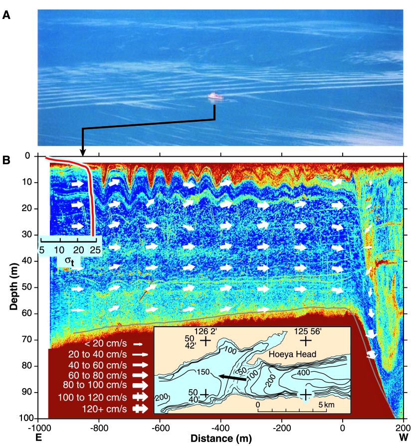
Figure 41: A shoaling internal undular bore in Knight Inlet, British Columbia, Canada. (a) Ship traversing internal waves with (b) associated current vectors and echo sounder profile, revealing the internal DSW structure. From [224]. Reprinted with permission from AAAS.

The canonical model for the description of weakly nonlinear long dispersive wave propagation over slowly varying topography is the variable-coefficient KdV equation (see, e.g., [227] and references therein),

$$u_{\tau}+\mu(\tau)uu_{\xi}+\lambda(\tau)u_{\xi\xi\xi}=0\,.$$ (7.1)

Here, $u$ is the normalized amplitude of the dominant mode in the waveguide, $\tau$ is related to the physical spatial variable $x$ and measures time along the spatial path of the wave, while $\xi$ is the temporal variable measuring the wave phase. The slowly varying coefficients $\mu(\tau)$ and $\lambda(\tau)$ are both expressed in terms of the variable topography profile $h(\tau)$. The equation (7.1) can be re-cast in an equivalent form of the constant-coefficient KdV equation with a small perturbation [228],

$$U_{t}+UU_{x}+U_{xxx}=\delta R(U,t),\quad\delta\ll 1,$$ (7.2)

where $U,x,t$ are new variables related to $u,\tau,\xi$ in (7.1), and the value of the perturbation parameter $\delta$ is determined by the typical inhomogeneity gradient (variable topography), $h^{\prime}(\tau)$. The presence of small dissipative terms in the original equation describing, e.g., volume viscosity or turbulent bottom friction, leads to the same perturbed KdV equation (7.2) but with an appropriately modified perturbation term, possibly depending upon derivatives of $U$. Thus one arrives at the prototypical problem of describing a DSW in the perturbed KdV equation and in perturbed dispersive-hyrodynamic models in general.

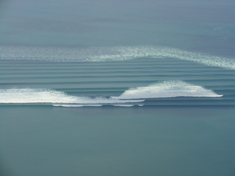
Figure 42: Shoaling of a tsunami off the island Koh Jum, Thailand (copyright Anders Grawin, 2006).

The modulation equations for perturbed dispersive hydrodynamic equations can be derived by averaging the balance laws of the perturbed equation, e.g., the KdVB equation, over the periodic family of the unperturbed equation, e.g., the KdV equation. Modulation systems for the perturbed KdV equation with different perturbation types, typically dissipative, were derived by various authors using either Whitham’s original prescription [53, 119] or direct multiple scales analysis [229]. In all cases, the result of the derivation is a non-homogeneous modulation system of the form

$$\frac{\partial r_{j}}{\partial t}+V_{j}({\bf r})\frac{\partial r_{j}}{\partial x}=\delta R_{j}({\bf r},t),\quad j=1,2,3,$$ (7.3)

where $V_{j}({\bf r})$ are the KdV-Whitham characteristic velocities eq. (2.53) and $R_{j}({\bf r},t)$ arise from averaging the perturbations in the governing equation’s balance laws. An effective general method for the derivation of modulation systems for perturbed integrable equations whose perturbation-free part belongs to the AKNS hierarchy was developed by Kamchatnov in [230]. See also [231] for a very recent extension of the original method.

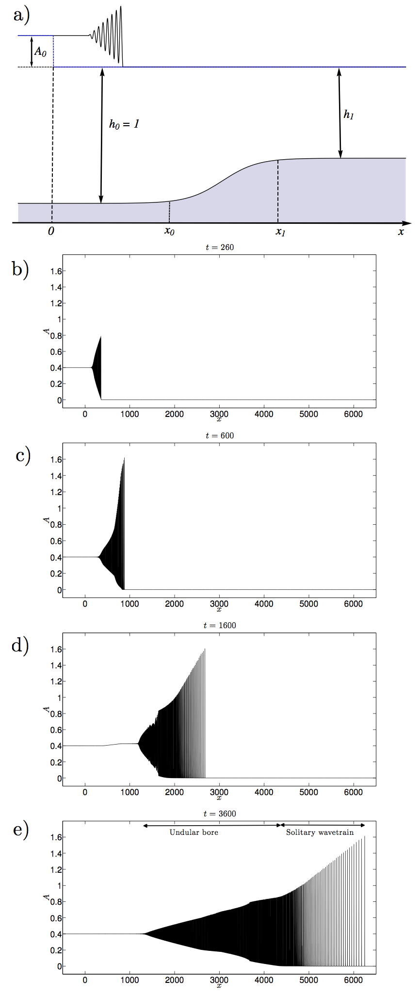
Figure 43: Transformation of a shallow water DSW (undular bore) propagating over a gentle bottom slope (Reprinted with permission from [235], copyright Cambridge University Press, 2012). a) schematic of the setting; b) - e) Numerical simulation of the variable coefficient KdV equation with DSW initial condition generated by an initial step in the flat bottom region. DSW interaction with shoaling topography leads to the generation of a large-amplitude solitary wavetrain propagating ahead of the DSW.

Unlike the unperturbed modulation system (2.51), the perturbed system (7.3) can possess TW solutions $\mathbf{r}(x-st)$ if the perturbation term does not depend on time, e.g., the KdVB equation (1.7). It was shown in [119, 53] that the TW solution of the KdVB-Whitham system connects two constant, disparate states: $u\to u_{\pm}$ as $x\to\pm\infty$, $u_{-}>u_{+}$, and satisfies the Rankine-Hugoniot condition $s=(u_{-}+u_{+})/2$. Thus, this solution describes slow modulations of a classical diffusive-dispersive shock wave in the small diffusion regime. As a matter of fact, this outlined construction of the TW modulation solution is equivalent to a direct multiple scales perturbation analysis of the ODE (1.8) with $\delta\ll 1$ for the TW solutions of the KdVB equation itself (see [51] and Sec. 5). However, modulation theory provides a much broader platform, enabling one to describe different stages of diffusive-dispersive shock development (see [60, 40]).

The TW solutions of the perturbed, integrable Whitham equations describing modulations of stationary, diffusive-dispersive shocks were obtained for the Kaup-Boussinesq-Burger’s equations [232], Benjamin-Ono-Burger’s equation [233], and the defocusing NLS equation with linear damping [234]. The unsteady dynamics of DSWs in perturbed systems, particularly in the variable-coefficient KdV equation (7.1), has only begun to be understood [228, 235]. In particular, the study of a shoaling shallow water DSW in [235] showed that, along with an adiabatic deformation of the DSW due to slowly varying topography, there is a non-adiabatic response (the generation of a sequence of isolated solitons): an expanding, large-amplitude, modulated solitary wavetrain propagating ahead of the DSW (see Fig. 43). Interestingly, a similar effect was observed in the overtaking interaction of a DSW and a rarefaction wave in [236] in the constant-coefficient KdV equation (cf. Fig. 37). These qualitative similarities between two apparently different problems are not surprising when one observes that, in our present formulation, the shallow water DSW essentially propagates through a “rarefaction region” of decreasing depth.

8 Resonant generation of DSWs in forced systems

We have described DSWs forming as a result of dispersive regularization of wavebreaking or Riemann initial data. Another DSW generation mechanism due to a moving piston was described in Sec. 3.3.4 where the DSW is realized by introducing a forcing term in the equation as a moving, impenetrable, sharp potential barrier [132]. If the forcing term is instead a moving potential barrier of finite width, a penetrable barrier, DSWs are generally not generated unless the barrier velocity is sufficiently close to the local speed of linear long waves in the reference frame of the barrier. In this case, the possibility arises for a new, resonant, mechanism of DSW generation, which is realized in a broad range of applications. This resonant mechanism was first identified and described in the framework of near-critical dispersive shallow water flows past broad, localized obstacles by Grimshaw and Smyth (GS) [237] and Smyth [238]. An appropriate model is the forced KdV equation, which can be obtained in the canonical form:

$$-A_{t}-\Delta A_{x}+6AA_{x}+A_{xxx}+F_{x}(x)=0.$$ (8.1)

Here $A$ denotes an appropriate field variable (e.g., the free-surface or interfacial displacement), $\Delta$ is the deviation of the incident flow velocity from the long wave phase speed and $F(x)\geq 0$ represents localized topographic forcing, that is we assume that

$$F(x)\to 0\quad\mathrm{as}\quad x\to\pm\infty.$$ (8.2)

In practice, it is sufficient to assume that $F(x)\geq 0$ for $x\leq l$ and is zero otherwise, with a single maximum at $x=0$. It is also assumed that $A(x,0)=0$ and $A\to 0$ as $|x|\to\infty$. A typical solution of the forced KdV equation (8.1) at exact criticality $\Delta=0$ is shown in Fig. 44.

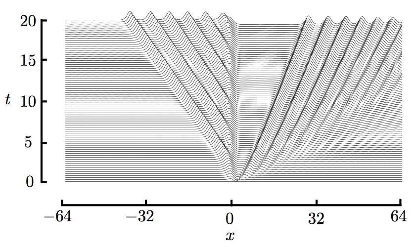
Figure 44: Transcritical flow past localized topography: a numerical solution of the forced KdV equation (8.1) at exact criticality $\Delta=0$. The partial, attached DSW is generated upstream (left) and a fully realized, detached DSW downstream (right).

The prominent feature of a near-critical flow past broad ($l\gg 1$) obstacles is the formation of a smooth, steady hydraulic transition over the obstacle region so that the flow is subcritical, $A\to A_{-}>0$, in front of the obstacle and supercritical, $A\to A_{+}<0$, after the obstacle. The transition between $A_{-}$ upstream and $A_{+}$ downstream is described by the steady, dispersionless hydraulic limit of (8.1),

$$-\Delta A_{x}+6AA_{x}+F_{x}(x)=0,$$ (8.3)

augmented by the condition of exact criticality at the maxumum of the forcing, expressed as the requirement that $A_{x}\neq 0$ when $F_{x}=0$ [237]. One can establish that the required heteroclinic solution of (8.3) exists only if

$$-(12F_{m})^{1/2}\leq\Delta\leq(12F_{m})^{1/2},$$ (8.4)

where $F_{m}=\max[F(x)]=F(0)$, and

$$6A_{\pm}=\Delta\mp(12F_{m})^{1/2}.$$

Outside the interval (8.4), the flow is either purely subcritical or purely supercritical, and in both cases is described by a homoclinic solution of (8.3) smoothly connecting the equilibrium states $A=0$ as $x\to\pm\infty$.

In the transcritical regime (8.4), the non-equilibrium upstream and downstream states $A_{\pm}$ are resolved back into the equilibrium state $A=0$ away from the obstacle with the aid of DSWs, propagating upstream and downstream. These are asymptotically described by the appropriate GP similarity modulation solutions of the unforced KdV equation, as these DSWs are formed away from the obstacle. Upstream DSW propagation is a remarkable feature of dispersive transcritical flows which does not have a counterpart in hyperbolic conservation law theory. Another important feature is that the asymptotic description of transcritical flow is defined by just two parameters, $\Delta$ and $F_{m}$, and does not depend on the detailed form of the obstacle.

The outlined GS analytical framework for the study of transcritical dispersive hydrodynamic flows proved to be quite general (see, e.g., [239, 240]). In the fluid mechanics context, it was successfully applied to the description of resonant generation of atmospheric internal waves (the Morning Glory, see Fig. 2) using the forced Benjamin-Ono equation [241]. Note that the modulation theory for Benjamin-Ono DSWs was developed in [242]. Resonant generation of internal waves in the framework of the forced Gardner equation was studied in [222], where, due to non-convexity of the hyperbolic flux (see Sec. 5), a rich variety of transcritical regimes were shown to be possible, including non-classical DSWs (kinks, contact DSWs) along with standard, KdV type, DSWs. One such regime with a kink-rarefaction double wave generated upstream and a classical DSW propagating downstream is shown in Fig. 45. The resonant generation of finite-amplitude shallow water DSWs in the framework of the forced Serre system was studied in [243] where the upstream and downstream DSW closure was performed using the results of the DSW fitting method applied to the unperturbed Serre equations [192] (see Sec. 4.2.2).

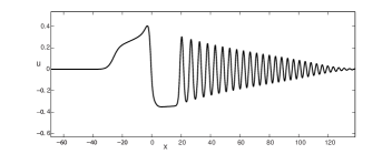
Figure 45: Transcritical internal wave flow past localized topography. Numerical solution of the forced Gardner equation with a kink-rarefaction generated upstream and a detached DSW downstream. Figure reproduced with permission from [222].

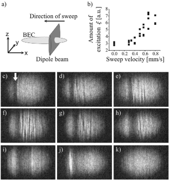
Figure 46: Demonstration of transcritical flow in a BEC induced by sweeping a repulsive laser beam. Reprinted figures with permission from [245] copyright 2007 by the American Physical Society.

DSW generation by transcritical flows past obstacles has been observed in superfluids and nonlinear optical media. The possibility of resonant generation of unsteady wavetrains in superfluid flows through broad, penetrable potential barriers was predicted by Hakim [244], who considered the forced, defocusing NLS equation, i.e., the Gross-Pitaevskii equation (3.59). The subcritical, transcritical and supercritical regimes were identified by analyzing the hydraulic solution obtained in the framework of shallow-water theory. The generation of unsteady wavetrains (DSWs) signifying the breakdown of superfluidity was studied numerically.

The resonant generation of dark soliton trains in 1D BEC flows past penetrable barriers has been realized experimentally in [245]. In the experiment, a wide, repulsive penetrable barrier created by a laser beam was swept at a constant speed through an elongated BEC confined to a cigar-shaped trap, as illustrated schematically in Fig.46a. The panels c) - k) in Fig. 46 show absorption images of the BEC density for different speeds of the dipole barrier. For very slow sweep speeds, such as in panel c), the part of the BEC through which the dipole beam was swept appears essentially unaffected (superfluidity maintained). The only visible effect of the beam is a density suppression that it leaves at its end position shown by the white arrow. At intermediate speeds, the shedding of dark solitons was observed (panels d) – g)) followed by a gradual decreasing of the number of generated solitons (panels h), i)) and an apparent full restoration of superfluidity at sufficiently large speeds (panel k)). These dynamics are in qualitative agreement with the predictions of the transcritical flow analysis in [244]. A detailed theory of resonant 1D NLS flows past wide penetrable barriers was constructed in [246] by extending the GS analytical framework to the forced NLS equation. In [246], the modulation solutions of the defocusing NLS equation (see Sec. 3.3), the potential-free Gross-Pitaevskii equation (3.59), were used for the description of the downstream and upstream DSWs connected by a smooth hydraulic solution. The downstream, almost stationary DSW adjacent to the potential was identified as a counterpart of the dark soliton train observed in the experiment [245].

In the nonlinear optics context, DSW generation via the nonlinear tunneling of a plane wave through a penetrable barrier potential was observed in [247].

9 Supersonic dispersive flows past obstacles and 2D oblique DSWs

Formation of shocks in multidimensional supersonic flows past obstacles is a textbook problem in classical shock theory [141, 136]. It is well-known that a two-dimensional (2D) supersonic flow, when turned through a compression, e.g., by an obstacle, can lead to the formation of a stationary viscous shock. Straight, oblique, and curved detached shocks can form when the flow is supersonic or transonic, respectively. These stationary shock patterns can exhibit stable, rich dynamical behavior [248] so finding their counterparts in dispersive hydrodynamics is a natural task with applications in water waves, superfluids and optics. Two examples of experimentally observed, 2D stationary oblique DSWs in supersonic dispersive-hydrodynamic flows past obstacles are presented in Fig. 47.

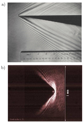
Figure 47: Experimental observations of 2D oblique DSWs. a) Oblique DSW in supercritical shallow water flow past obstacle [249]. Reprinted from [249] with permission from Elsevier. b) BEC bow shock from expansion past an obstacle. Reprinted figure with permission from [250] copyright 2006 by the American Physical Society.

Assuming steady, irrotational, 2D dispersive hydrodynamic motion, the governing Eulerian equations (1.1) become a PDE system for three quantities: the density $\rho(x,y)$ and two velocity components ${\mathbf{u}}=(u(x,y),v(x,y))$. For example, the dispersive-hydrodynamic representation of the stationary, 2D defocusing NLS equation has the form:

$$\begin{split}(\rho u)_{x}+(\rho v)_{y}=0,\\ uu_{x}+vu_{y}+\rho_{x}+\left(\frac{\rho_{x}^{2}+\rho_{y}^{2}}{8\rho^{2}}-\frac{\rho_{xx}+\rho_{yy}}{4\rho}\right)_{x}=0,\\ uv_{x}+vv_{y}+\rho_{y}+\left(\frac{\rho_{x}^{2}+\rho_{y}^{2}}{8\rho^{2}}-\frac{\rho_{xx}+\rho_{yy}}{4\rho}\right)_{y}=0,\\ u_{y}-v_{x}=0\,.\end{split}$$ (9.1)

We introduce the Mach number $M=|{\bf u}|/c$, where $c(\rho)=\sqrt{P^{\prime}(\rho)}$ is the speed of sound in the long-wave, dispersionless limit. For NLS dispersive hydrodynamics, $c=\sqrt{\rho}$. The dispersionless limit of (9.1) is hyperbolic if $M>1$ corresponding to supersonic flow. This hyperbolicity condition holds for general, 2D dispersionless Euler systems under appropriate monotonicity conditions on the pressure law $P(\rho)$ [141]. In certain application areas, e.g., shallow water waves, the condition $M>1$, e.g., Froude number above unity, is termed supercritical.

We now consider a stationary, supersonic flow past an impenetrable obstacle in the uppper half-plane by introducing appropriate boundary conditions for the 2D dispersive Eulerian systems. We shall be using equations (9.1) as an instructive and representative example. See Fig. 48 for a schematic of the configuration considered.

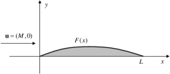
Figure 48: Schematic of 2D flow past an obstacle.

Let the shape of the obstacle be given by $y=F(x)\geq 0$ for $x\geq 0$, $F(0)=0$. Assuming hyperbolicity of the problem, the flow in the lower half-plane is isolated from the flow in the upper half plane so can be considered independently. The impenetrability condition ${\bf u}\cdot{\bf n}|_{S}=0$ at the obstacle’s surface assumes the form

$$v=uF^{\prime}(x)\quad\text{at}\quad y=F(x).$$ (9.2)

We also impose the condition of stationary equilibrium flow far away from the obstacle

$$\rho=1,\quad u=M,\quad v=0\quad\text{at}\quad|x|,|y|\to\infty.$$ (9.3)

The system (9.1) has a family of stationary, periodic solutions [251] and is amenable, in principle, to a general modulation analysis using the DSW fitting method. Care must be taken due to the presence of a 2D convective instability [252, 253], a feature, not occuring in 1D flows.

Since the general problem (9.1) - (9.3) is quite involved, it is instructive to consider first some more manageable approximations by introducing reasonable small/large parameters.

9.1 Supersonic flow past slender obstacles: weakly nonlinear KdV approximation

If the obstacle is slender, $\varepsilon=\max|F^{\prime}(x)|\ll 1$, one can use multiple scales expansions for (9.1), reducing the boundary value problem (9.1) - (9.3) to an initial value problem for the KdV equation. This has been done for a rather general dispersive hydrodynamic setting in [66] and, later, in [254]. To this end, we introduce the asymptotic expansions [251, 253],

$$\begin{split}\rho&=1+\varepsilon\rho_{1}+\varepsilon^{2}\rho_{2}+\ldots,\\ u&=M+\varepsilon u_{1}+\varepsilon^{2}\rho_{2}+\ldots,\\ v&=\varepsilon v_{1}+\varepsilon^{2}v_{2}+\ldots,\end{split}$$ (9.4)

$\rho_{i},u_{i},v_{i}\to 0$ as $x,y\to\infty$, along with new independent variables

$$\zeta=x-\sqrt{M^{2}-1}y,\quad\tau=\varepsilon y.$$ (9.5)

Substitution of (9.4), (9.5) into (9.1) yields, at the first order in $\varepsilon$,

$$u_{1}=-\frac{\rho_{1}}{M},\quad v_{1}=\frac{\sqrt{M^{2}-1}}{M}\rho_{1},$$ (9.6)

Continuing to the second order, we obtain the KdV equation for $\rho_{1}$:

$$\rho_{1,\tau}-\frac{3M^{2}}{2\sqrt{M^{2}-1}}\rho_{1}\rho_{1,\zeta}+\frac{M^{4}}{8\sqrt{M^{2}-1}}\rho_{1,\zeta\zeta\zeta}=0.$$ (9.7)

The boundary condition (9.2) yields, at the same order in $\varepsilon$, the KdV initial condition

$$\rho_{1}(0,\zeta)=-\frac{M^{2}}{\sqrt{M^{2}-1}}F^{\prime}(\zeta).$$ (9.8)

Thus the boundary value problem (9.1) - (9.3) for the 2D stationary NLS equation is reduced to the KdV initial value problem (9.7), (9.8). One can see from (9.8) that flow past a straight corner yields the Riemann step problem, while flow past an airfoil corresponds to the evolution of a bi-polar profile and $N$-wave type evolution. See Sec. 3.2.4 and note the change of dispersion sign in (9.7) resulting in wave pattern inversion, in both polarity and orientation. The standard similarity DSW of the KdV Riemann problem (Sec. 3.1) then maps to the 2D oblique DSW in the $(x,y)$-plane, with an oblique dark soliton [255] at the edge facing the corner and a stationary 2D linear wavepacket at the opposite, harmonic edge. A typical solution of NLS flow past a corner is shown in Fig. 49.

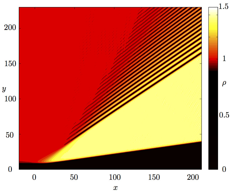
Figure 49: Numerical solution of the 2D NLS equation yielding a steady, oblique DSW in supercritical flow past a corner.

The detailed study of the KdV approximation in supersonic dispersive-hydrodynamic flow past obstacles has been undertaken in [254, 126].

9.2 Hypersonic flow: NLS piston problem approximation

If the oncoming flow is highly supersonic, $M\gg 1$, the steady problem of two-dimensional flow past a slender body can be asymptotically transformed to the much simpler problem of 1D “unsteady” flow along the $y$ axis with the scaled $x$-coordinate playing the role of time [256]. This notion of hypersonic similitude is well-known in classical gas dynamics (see, e.g., [257]). To this end, we substitute into eqs. (9.1) the expansion

$$u=M+u_{1}+O(1/M),\quad T=x/M,\quad Y=y,$$ (9.9)

assuming $M^{-1}\ll 1$. Then to leading order we obtain

$$\begin{split}\rho_{T}+(\rho v)_{Y}=0,\\ v_{T}+vv_{Y}+\rho_{Y}+\left(\frac{\rho_{Y}^{2}}{8n^{2}}-\frac{\rho_{YY}}{4\rho}\right)_{Y}=0,\end{split}$$ (9.10)

$$u_{1}=0.$$

Equations (9.10) represent the hydrodynamic form of the 1D defocusing NLS equation

$$i\Psi_{T}+\tfrac{1}{2}\Psi_{YY}-|\Psi|^{2}\Psi=0$$ (9.11)

for the complex field variable

$$\Psi=\sqrt{\rho}\exp\left(i\int^{Y}v(Y^{\prime},T)dY^{\prime}\right),$$ (9.12)

and so we can apply the modulation theory developed in Sec. 3.3. It is remarkable that, if $M\alpha=O(1)$, where $\alpha=\mathrm{max}|F^{\prime}(x)|$, the boundary condition (9.2) asymptotically reduces to the piston problem with moving boundary condition

$$v=v_{p}=df/dT\quad\text{at}\quad Y=f(T),$$ (9.13)

where the piston motion is given by the function $f(T)=F(MT)$ describing the obstacle’s profile. Conditions (9.3) at infinity transform into

$$\rho=1,\ \ v=0\quad\hbox{as}\ \ Y\to\infty\,.$$ (9.14)

Thus the problem of hypersonic, steady 2D NLS flow past a slender body has been reduced to the 1D unsteady piston problem, whose solutions were obtained in Sec. 3.3.4. The piston analogy is illustrated in Fig. 50.

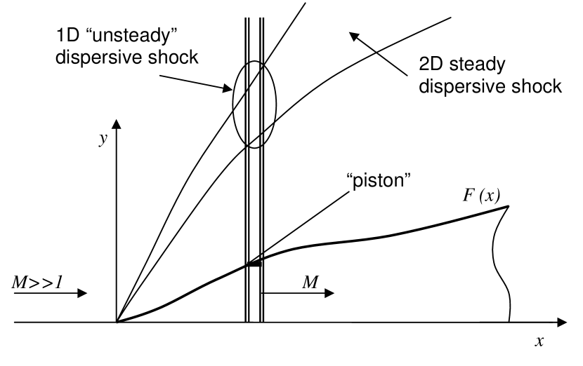
Figure 50: Piston analogy in hypersonic flow past an obstacle. Reprinted figure with permission from [140] copyright 2009 by the American Physical Society.

The piston approximation, similar to the KdV approximation considered in the previous subsection, is valid for slender obstacles, $\alpha\ll 1$. The important difference, however, is that the piston approximation does not contain a small amplitude assumption. Indeed, there is no small-amplitude expansion for $\rho$ involved and $u_{1}=O(1)$ in (9.9), which enables one to capture large-amplitude effects such as cavitation (see Sec. 3.3.2), which are not present in the KdV approximation.

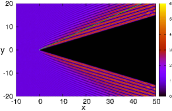
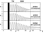
Figure 51: Hypersonic ($M=10$) 2D NLS flow past a wedge with the opening angle $2\alpha=0.6$: a) density plot. The green dashed line in the upper half-plane marks the end of the periodic transition wave predicted by the modulation theory. b) profile $\rho(y)$ at $x=30$; top: analytical modulation theory solution; middle: numerical solution of the associated 1D piston problem; bottom: 1D cut of the full 2D solution at $t=15$. Points $y^{-}$ and $y^{+}$ mark the boundaries of the DSW specified by the modulation solution. The wedge surface in the upper half-plane (the piston) is located at about $y=9$. Reprinted figure with permission from [140] copyright 2009 by the American Physical Society.

Modulation theory of NLS 2D hypersonic flow past obstacles was developed in [258, 259, 140]. Comparison of the modulation theory results for hypersonic flow past a corner exhibiting large-amplitude cavitation effects is shown in Fig. 51. The numerical simulation of hypersonic flow past an airfoil is shown in Fig. 52. One can see the formation of two oblique DSWs with contrasting asymptotic properties: the rear DSW transforms into a train (fan) of oblique dark solitons, while the front one asymptotically assumes a universal “BEC ship-wave” pattern [260], obtained by the application of Kelvin’s famous construction for linear deep water waves [1] to the 2D NLS equation. The analogy with dispersive-hydrodynamic $N$-wave evolution is, again, helpful in the interpretation of the global wave pattern arising in flow past an airfoil.

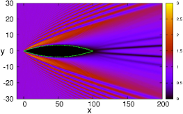
Figure 52: 2D hypersonic NLS flow past an airfoil. Reprinted figure with permission from [140] copyright 2009 by the American Physical Society.

In conclusion of this section, we mention that, along with steady oblique DSWs, 2D dispersive hydrodynamics admits unsteady oblique DSWs, which result from an initial value problem and arise as an initial pattern in the development of steady oblique DSWs. These unsteady oblique DSWs were studied in [261]

10 Conclusion

Dispersive shock waves have recently become the subject of very active research due to the growing recognition of their fundamental nature and ubiquity in applications, which is comparable to the ubiquity of solitons. This recognition, which had been steadily present in water wave theory, has been recently facilitated by groundbreaking experiments in superfluids and nonlinear optics. The very recent progress in dynamics of viscous fluid conduits has made DSWs readily available for detailed quantitative measurements.

This review represents an attempt to summarize the results of the last 50 years of DSW research using the framework of nonlinear modulation theory pioneered by Whitham in 1965. The Whitham method of slow modulations and the Gurevich-Pitaevskii matching regularization problem have provided a powerful theoretical framework for the development of DSW theory, encompassing both integrable and non-integrable dispersive-hydrodynamic systems.

References

- [1] G. B. Whitham, Linear and nonlinear waves, Wiley, New York, 1974.
- [2] Z. Dutton, M. Budde, C. Slowe, L. V. Hau, Observation of quantum shock waves created with ultra-compressed slow light pulses in a Bose-Einstein condensate, Science 293 (2001) 663.
- [3] T. P. Simula, P. Engels, I. Coddington, V. Schweikhard, E. A. Cornell, R. J. Ballagh, Observations on sound propagation in rapidly rotating Bose-Einstein condensates, Phys. Rev. Lett. 94 (2005) 080404.
- [4] M. A. Hoefer, M. J. Ablowitz, I. Coddington, E. A. Cornell, P. Engels, V. Schweikhard, Dispersive and classical shock waves in Bose-Einstein condensates and gas dynamics, Phys. Rev. A 74 (2006) 023623.
- [5] J. J. Chang, P. Engels, M. A. Hoefer, Formation of dispersive shock waves by merging and splitting Bose-Einstein condensates, Phys. Rev. Lett. 101 (2008) 170404.
- [6] M. A. Hoefer, P. Engels, J. Chang, Matter-wave interference in Bose-Einstein condensates: A dispersive hydrodynamic perspective, Physica D 238 (15) (2009) 1311–1320.
- [7] R. Meppelink, S. B. Koller, J. M. Vogels, P. van der Straten, E. D. van Ooijen, N. R. Heckenberg, H. Rubinsztein-Dunlop, S. A. Haine, M. J. Davis, Observation of shock waves in a large Bose-Einstein condensate, Phys. Rev. A 80 (4) (2009) 043606–7.
- [8] J. E. Rothenberg, D. Grischkowsky, Observation of the formation of an optical intensity shock and wave breaking in the nonlinear propagation of pulses in optical fibers, Phys. Rev. Lett. 62 (5) (1989) 531.
- [9] G. Couton, H. Maillote, M. Chauvet, Self-formation of multiple spatial photovoltaic solitons, J. Opt. B: Quantum Semiclass. Opt. 6 (2004) S223–S230.
- [10] W. Wan, S. Jia, J. W. Fleischer, Dispersive superfluid-like shock waves in nonlinear optics, Nat. Phys. 3 (1) (2007) 46–51.
- [11] S. Jia, W. Wan, J. W. Fleischer, Dispersive shock waves in nonlinear arrays, Phys. Rev. Lett. 99 (22) (2007) 223901–4.
- [12] C. Barsi, W. Wan, C. Sun, J. W. Fleischer, Dispersive shock waves with nonlocal nonlinearity, Opt. Lett. 32 (20) (2007) 2930–2932.
- [13] N. Ghofraniha, C. Conti, G. Ruocco, S. Trillo, Shocks in nonlocal media, Phys. Rev. Lett. 99 (2007) 043903.
- [14] C. Conti, A. Fratalocchi, M. Peccianti, G. Ruocco, S. Trillo, Observation of a gradient catastrophe generating solitons, Phys. Rev. Lett. 102 (8) (2009) 083902.
- [15] N. Ghofraniha, L. S. Amato, V. Folli, S. Trillo, E. DelRe, C. Conti, Measurement of scaling laws for shock waves in thermal nonlocal media, Opt. Lett. 37 (12) (2012) 2325–2327.
- [16] J. Fatome, C. Finot, G. Millot, A. Armaroli, S. Trillo, Observation of optical undular bores in multiple four-wave mixing, Phys. Rev. X 4 (2014) 021022.
- [17] E. Rolley, C. Guthmann, M. S. Pettersen, The hydraulic jump and ripples in liquid helium, Physica B 394 (1) (2007) 46–55.
- [18] Y. C. Mo, R. A. Kishek, D. Feldman, I. Haber, B. Beaudoin, P. G. O’Shea, J. C. T. Thangaraj, Experimental observations of soliton wave trains in electron beams, Phys. Rev. Lett. 110 (8) (2013) 084802.
- [19] R. J. Taylor, D. R. Baker, H. Ikezi, Observation of collisionless electrostatic shocks, Phys. Rev. Lett. 24 (1970) 206–209.
- [20] M. Q. Tran, K. Appert, C. Hollenstein, R. W. Means, J. Vaclavik, Shocklike solutions of the Korteweg-de Vries equation, Plasma Phys. 19 (1977) 381.
- [21] P. M. Bazin, Recherches experimentales sur la propagation des ondes (Experimental research on wave propagation), Mem. Pres. Acad. Sci., Paris 19 (1865) 495–644.
- [22] J. L. Hammack, H. Segur, The Korteweg-de Vries equation and water waves. Part 3. Oscillatory waves, J. Fluid Mech. 84 (02) (1978) 337–358.
- [23] A. Treske, Undular bores (Favre-waves) in open channels - experimental studies, J. Hyd. Res. 32 (3) (1994) 355–370.
- [24] P. A. Madsen, D. R. Fuhrman, H. A. Schäffer, On the solitary wave paradigm for tsunamis, J. Geophys. Res. 113 (2008) C12012.
- [25] H. Chanson, Current knowledge in hydraulic jumps and related phenomena. A survey of experimental results, Euro. J. Mech. B 28 (2) (2009) 191–210.
- [26] H. Chanson, Tidal Bores, Aegir, Eagre, Mascaret, Pororoca: Theory and Observations, World Scientific, Singapore, 2011.
- [27] S. Trillo, M. Klein, G. F. Clauss, M. Onorato, Observation of dispersive shock waves developing from initial depressions in shallow water, Physica D (2016) doi:10.1016/j.physd.2016.01.007.
-
[28]
J. R. Apel, Oceanic
internal waves and solitons, Prepared for Office of Naval Research
Code 322 PO, Global Ocean Associates (2002).
URL http://www.internalwaveatlas.com/Atlas2_index.html - [29] A. Scotti, Observation of very large and steep internal waves of elevation near the Massachusetts coast, Geophys. Res. Lett. 31 (22) (2004).
- [30] C. Wang, R. Pawlowicz, Propagation speeds of strongly nonlinear near-surface internal waves in the Strait of Georgia, J. Geophys. Res. 116 (C10) (2011) C10021.
- [31] N. F. Smyth, P. E. Holloway, Hydraulic jump and undular bore formation on a shelf break, J. Phys. Oceanogr. 18 (7) (1988) 947–962.
- [32] D. R. Christie, The morning glory of the Gulf of Carpentaria: a paradigm for non-linear waves in the lower atmosphere, Austral. Met. Mag. 41 (1992) 21–60.
- [33] M. O. G. Hills, D. R. Durran, Nonstationary trapped lee waves generated by the passage of an isolated jet, J. Atmos. Sci. 69 (2012) 3040–3059.
- [34] J. A. Whitehead, K. R. Helfrich, Magma waves and diapiric dynamics, in: M. P. Ryan (Ed.), Magma Transport and Storage, John Wiley & Sons, Chichester, UK, 1990, pp. 53–76.
- [35] N. K. Lowman, M. A. Hoefer, Dispersive shock waves in viscously deformable media, J. Fluid Mech. 718 (2013) 524–557.
- [36] J. Grue, E. N. Pelinovsky, D. Fructus, T. Talipova, C. Kharif, Formation of undular bores and solitary waves in the Strait of Malacca caused by the 26 December 2004 Indian Ocean tsunami, J. Geophys. Res. 113 (2008) C05008.
- [37] J. Boussinesq, Essai sur la theorie des eaux courantes, Mem. pres. div. Sav. Acad. Sci. Inst. Fr. 23 (1877) 1.
- [38] D. J. Korteweg, G. de Vries, On the change of form of long waves advancing in a rectangular canal, and on a new type of long stationary waves, Phil. Mag. Ser. 5 39 (240) (1895) 422–443.
- [39] L. A. Ostrovsky, Asymptotic perturbation theory of waves, Imperial College Press, London, 2014.
- [40] G. A. El, M. A. Hoefer, M. Shearer, Dispersive and diffusive-dispersive shock waves for nonconvex conservation laws, arXiv:1501.01681 [nlin.PS].
- [41] P. D. Lax, Hyperbolic systems of conservation laws and the mathematical theory of shock waves, SIAM, 1973.
- [42] T. B. Benjamin, M. J. Lighthill, On cnoidal waves and bores, Proc. Roy. Soc. Lond. A 224 (1159) (1954) 448–460.
- [43] S. S. Moiseev, R. Z. Sagdeev, Collisionless shock waves in a plasma in a weak magnetic field, J. Nucl. Energy C 5 (1963) 43–47.
- [44] R. Z. Sagdeev, Cooperative phenomena and shock waves in collisionless plasmas, Rev. Plasma Phys. 4 (1966) 23.
- [45] R. Z. Sagdeev and C. F. Kennel, Collisionless shock waves, Scientific American, 264 (1991) 106–113.
- [46] H. Grad, P. N. Hu, Unified shock profile in a plasma, Phys. Fluids 10 (12) (1967) 2596–2602.
- [47] M. Kulkarni, A. G. Abanov, Hydrodynamics of cold atomic gases in the limit of weak nonlinearity, dispersion, and dissipation, Phys. Rev. A 86 (3) (2012) 033614.
- [48] G. B. Whitham, Non-linear dispersive waves, Proc. Roy. Soc. London A 283 (1965) 238–261.
- [49] A. V. Gurevich, L. P. Pitaevskii, Nonstationary structure of a collisionless shock wave, Sov. Phys. JETP 38 (2) (1974) 291–297, translation from Russian of A. V. Gurevich and L. P. Pitaevskii, Zh. Eksp. Teor. Fiz. 65, 590-604 (August 1973).
- [50] P. D. Lax, C. D. Levermore, The small dispersion limit of the Korteweg-de Vries equation: 1-3, Comm. Pure Appl. Math. 36 (3,5,6) (1983) 253–290; 571–593; 809–830.
- [51] R. S. Johnson, A non-linear equation incorporating damping and dispersion, J Fluid Mech. 42 (01) (1970) 49–60.
- [52] J. L. Bona, M. E. Schonbek, Travelling-wave solutions to the Korteweg-de Vries-Burgers equation, Proc. Roy. Soc. Edinburgh A 101 (3-4) (1985) 207–226.
- [53] A. V. Gurevich, L. P. Pitaevskii, Averaged description of waves in the Korteweg-de Vries-Burgers equation, Sov. Phys. JETP 66 (3) (1987) 490–495.
- [54] A. M. Kamchatnov, Nonlinear periodic waves and their modulations: an introductory course, World Scientific, 2000.
- [55] M. A. Hoefer, M. J. Ablowitz, Scholarpedia 4 (11) (2009) 5562.
- [56] G. A. El, Resolution of a shock in hyperbolic systems modified by weak dispersion, Chaos 15 (2005) 037103.
- [57] M. A. Hoefer, Shock waves in dispersive Eulerian fluids, J. Nonlinear Sci. 24 (3) (2014) 525–577.
- [58] B. Rozhdestvenskii, N. Janenko, Systems of quasilinear equations and their applications to gas dynamics, RI: American Mathematical Society, Providence, 1983.
- [59] C. M. Dafermos, Hyperbolic conservation laws in continuum physics, 3rd Edition, Springer, 2009.
- [60] B. A. Dubrovin, S. P. Novikov, Hydrodynamics of weakly deformed soliton lattices. Differential geometry and Hamiltonian theory, Russian Mathematical Surveys 44 (6) (1989) 35–124.
- [61] H. Flaschka, M. G. Forest, D. W. McLaughlin, Multiphase averaging and the inverse spectral solution of the Korteweg-de Vries equation, Comm. Pure Appl. Math. 33 (1980) 739–784.
- [62] S. P. Tsarev, Poisson brackets and one-dimensional Hamiltonian systems of hydrodynamic type, Sov. Math. Dokl. 31 (1985) 488–491.
- [63] N. N. Bogoliubov, Y. A. Mitropolsky, Asymptotic methods in the theory of non-linear oscillations, Hindustan Publishing Corp, 1961.
- [64] G. B. Whitham, A general approach to linear and non-linear dispersive waves using a Lagrangian, J. Fluid Mech. 22 (02) (1965) 273–283.
- [65] J. C. Luke, A perturbation method for nonlinear dispersive wave problems, Proc. Roy. Soc. London A 292 (1430) (1966) 403–412.
- [66] V. Karpman, Non-linear waves in dispersive media, Elsevier, Amsterdam, 1974.
- [67] L. A. Ostrovsky, A. I. Potapov, Modulated waves: theory and applications, Johns Hopkins Univ. Press, Baltimore, London, 1999.
- [68] E. Infeld, G. Rowlands, Nonlinear waves, solitons and chaos, Cambridhe Univ. Press, Cambridge, 2000.
- [69] M. J. Lighthill, Contributions to the theory of waves in non-linear dispersive systems, IMA J. Appl. Math. 1 (3) (1965) 269–306.
- [70] T. B. Benjamin, K. Hasselmann, Instability of periodic wavetrains in nonlinear dispersive systems, Proc. Roy. Soc. London A 299 (1456) (1967) 59–76.
- [71] V. Zakharov, L. Ostrovsky, Modulation instability: The beginning, Physica D 238 (5) (2009) 540–548.
- [72] M. J. Ablowitz, D. J. Benney, The evolution of multi-phase modes for nonlinear dispersive waves, Stud. Appl. Math. 49 (1970) 225–238.
- [73] A. V. Gurevich, A. L. Krylov, G. A. El, Breaking problem in dispersive hydrodynamics, JETP Lett. 54 (1991) 102–107.
- [74] V. R. Kudashev, Wave-number conservation and succession of symmetries during a Whitham averaging, JETP Lett. 54 (1991) 175–178.
- [75] M. J. Ablowitz, Nonlinear dispersive waves: asymptotic analysis and solitons, Cambridge Texts in Applied Mathematics, Cambridge University Press, Cambridge, UK, 2011.
- [76] D. J. Benney, A. C. Newell, Propagation of nonlinear wave envelopes, J. Math. Phys. 46 (2) (1967) 133–139.
- [77] A. Newell, Solitons in mathematics and physics, CBMS-NSF, SIAM, Philadelphia, PA, 1985.
- [78] T. J. Bridges, Breakdown of the Whitham modulation theory and the emergence of dispersion, Stud. Appl. Math. (2015) 1–18.
- [79] C. F. Driscoll, T. M. O’Neil, Modulational instability of cnoidal wave solutions of the modified Korteweg-de Vries equation, J. Math. Phys. 17 (7) (1975) 1196–1200.
- [80] R. M. Miura, Korteweg-de Vries equation and generalizations. i. a remarkable explicit nonlinear transformation, J. Math. Phys. 9 (8) (1968) 1202–1204.
- [81] M. G. Forest, J. Lee, Geometry and modulation theory for the periodic nonlinear Schrödinger equation, in: C. D. et. al (Ed.), Oscillation Theory, Computation, and Methods of Compensated Compactness, Vol. 2, Springer, 1986, pp. 35–69.
- [82] M. V. Pavlov, Nonlinear Schrödinger equation and the Bogolyubov-Whitham method of averaging, Teor. Mat. Fiz. 71 (3) (1987) 351–356, english translation in Theor. Math. Phys. 71 (1987) 584–588.
- [83] G. A. El, R. H. J. Grimshaw, M. V. Pavlov, Integrable Shallow water equations and undular bores, Stud. Appl. Math. 106 (2) (2001) 157–186.
- [84] E. D. Belokolos, A. I. Bobenko, V. Z. Enolski, A. R. Its, V. B. Matveev, Algebro-geometric approach to nonlinear integrable equations, Springer, New York, 1994.
- [85] I. M. Krichever, Method of averaging for two-dimensional ”integrable” equations, Func. Anal. Appl. 22 (3) (1989) 200–213.
- [86] A. M. Kamchatnov, New approach to periodic solutions of integrable equations and nonlinear theory of modulational instability, Phys. Rep. 286 (1997) 199–270.
- [87] M. J. Ablowitz, D. J. Kaup, A. C. Newell, H. Segur, The inverse scattering transform-Fourier analysis for nonlinear problems, Stud. Appl. Math. 53 (1974) 249–315.
- [88] P. Lax, Integrals of nonlinear equations of evolution and solitary waves, Comm. Pur. Appl. Math. 21 (1968) 467–490.
- [89] S. P. Novikov, S. Manakov, L. P. Pitaevskii, V. Zakharov, Theory of solitons: the inverse scattering method, Monographs in Contemporary Mathematics, Springer, 1984.
- [90] D. Levermore, The hyperbolic nature of the zero dispersion KdV limit, Commun. Part. Diff. Eq 13 (4) (1988) 495–514.
- [91] G. Darboux, Sur la theorie generale de surfaces, reprint Edition, Vol. II, Chelsea, 1972.
- [92] E. Copson, Partial differential equations, Cambridge University Press, Cambridge, 1975.
- [93] I. Hauser, F. Ernst, Initial value problem for colliding gravitational plane wave, J. Math. Phys. 30 (1989) 872–887.
- [94] L. Eisenhart, Triply conjugate systems with equal point invariants., Ann. Math. 20 (1919) 262–273.
- [95] V. R. Kudashev, S. E. Sharapov, Inheritance of KdV symmetries under Whitham averaging and hydrodynamic symmetries of the Whitham equations, Theor. Math. Phys. 87 (1) (1991) 358–363.
- [96] F.-R. Tian, Oscillations of the zero dispersion limit of the Korteweg-de Vries equation, Comm. Pure Appl. Math. 46 (8) (1993) 1093–1129.
- [97] T. Grava, C. Klein, Numerical solution of the small dispersion limit of Korteweg-de Vries and Whitham equations, Comm. Pure Appl. Math. 60 (11) (2007) 1623–1664.
- [98] G. A. El, A. L. Krylov, S. Venakides, Unified approach to KdV modulations, Comm. Pure Appl. Math. 54 (2001) 1243–1270.
- [99] P. Deift, S. Venakides, X. Zhou, An extension of the steepest descent method for Riemann-Hilbert problems: The small dispersion limit of the Korteweg-de Vries (KdV) equation, Proc. Nat. Acad. Sci. USA 95 (2) (1998) 450–454.
- [100] A. Shabat, V. Zakharov, Exact theory of two-dimensional self-focusing and one-dimensional self-modulation of waves in nonlinear media, Sov. Phys. JETP 34 (1) (1972) 62.
- [101] V. E. Zakharov, A. B. Shabat, Interaction between solitons in a stable medium, Sov. Phys. JETP 37 (5) (1973) 823–828.
- [102] G. El, V. Khodorovskii, A. Leszczyszyn, Refraction of dispersive shock waves, Physica D 241 (18) (2012) 1567–1587.
- [103] Y. Kodama, The Whitham equations for optical communications: mathematical theory of NRZ, SIAM J. Appl. Math. 59 (6) (1999) 2162–2192.
- [104] S. Jin, C. D. Levermore, D. W. McLaughlin, The semiclassical limit of the defocusing NLS hierarchy, Comm. Pure Appl. Math. 52 (5) (1999) 613–654.
- [105] M. Abramowitz, I. Stegun, Handbook of Mathematical Functions with Formulas, Graphs, and Mathematical Tables, Dover Publications, New York, 1972.
- [106] A. V. Gurevich, A. L. Krylov, G. A. El, Evolution of a Riemann wave in dispersive hydrodynamics, Sov. Phys. JETP 47 (1992) 957–962.
- [107] B. Riemann, Über die Fortpflanzung ebener Luftwellen von endlicher Schwingungsweite, Abh. d. Königl. Ges. d. Wiss. zu Göttingen 8 (1860) 43–65.
- [108] B. Fornberg, G. B. Whitham, A numerical and theoretical study of certain nonlinear wave phenomena, Phil. Trans. Roy. Soc. A 289 (1978) 373–404.
- [109] M. J. Ablowitz, D. E. Baldwin, Interactions and asymptotics of dispersive shock waves – Korteweg-de Vries equation, Phys. Lett. A 377 (7) (2013) 555–559.
- [110] E. Y. Khruslov, Asymptotics of the solution of the Cauchy problem for the Korteweg-de Vries equation with initial data of step type, Mat. Sb. (N. S.) 99 (141) (1976) 261–281.
- [111] A. V. Gurevich, A. L. Krylov, G. A. El, Nonlinear modulated waves in dispersive hydrodynamics, Sov. Phys. JETP 71 (5) (1990) 899–910.
- [112] J. A. Leach, D. J. Needham, The large-time development of the solution to an initial-value problem for the Korteweg-de Vries equation: I. Initial data has a discontinuous expansive step, Nonlinearity 21 (10) (2008) 2391–2408.
- [113] A. M. Bloch, Y. Kodama, Dispersive regularization of the Whitham equation for the Toda lattice, SIAM J. Appl. Math. 52 (1992) 909–928.
- [114] G. Biondini, Y. Kodama, On the Whitham equations for the defocusing nonlinear Schrödinger equation with step initial data, J. Nonlin. Sci. 16 (2006) 435–481.
- [115] L. Landau, E. Lifshitz, Quantum mechanics, Pergamon Press, 1965.
- [116] R. Courant, D. Hilbert, Methods of Mathematical Physics, Volume 1, Wiley, 1989.
- [117] G. Potëmin, Algebro-geometric construction of self-similar solutions of the Whitham equations, Russian Math. Surveys 43 (1988) 252–253.
- [118] O. C. Wright, M. Gregory Forest, K. T. R. McLaughlin, On the exact solution of the geometric optics approximation of the defocusing nonlinear Schrödinger equation, Phys. Lett. A 257 (3-4) (1999) 170–174.
- [119] V. V. Avilov, I. M. Krichever, S. P. Novikov, Evolution of a Whitham zone in the Korteweg-de Vries theory, Sov. Phys. Dokl. 32 (1987) 564–566.
- [120] A. Gurevich, A. Krylov, N. Mazur, Quasisimple waves in dispersive hydrodynamics, Sov. Phys. JETP 68 (1989) 966 – 974.
- [121] G. A. El, R. H. J. Grimshaw, Generation of undular bores in the shelves of slowly-varying solitary waves, Chaos 12 (4) (2002) 1015–1026.
- [122] F.-R. Tian, The initial value problem for the Whitham averaged system, Commun. Math. Phys. 166 (1994) 79–115.
- [123] P. D. Lax, C. D. Levermore, S. Venakides, The generation and propagation of oscillations in dispersive initial value problems and their limiting behavior, in: A. Fokas, V. E. Zakharov (Eds.), Important Developments in Soliton Theory, Springer, Berlin, 1994, pp. 205–241.
- [124] V. Karpman, An asymptotic solution of the Korteweg–de Vries equation, Phys. Lett. A 25 (1967) 708 – 709.
- [125] A. Krylov, V. Khodorovskii, G. El, Evolution of a nonmonotonic perturbation in Korteweg-de Vries hydrodynamics, JETP Lett. 56 (6) (1992) 323–327.
- [126] A. V. Gurevich, A. L. Krylov, V. V. Khodorovskii, G. A. El, Supersonic flow past finite-length bodies in dispersive hydrodynamics, Sov. Phys. JETP 82 (1996) 709–718.
- [127] T. Claeys, T. Grava, Solitonic asymptotics for the Korteweg-de Vries equation in the small dispersion limit, SIAM J. Math. Anal. 42 (5) (2010) 2132.
- [128] G. El, V. Khodorovsky, Evolution of a solitonless large-scale perturbation in Korteweg-de Vries hydrodynamics, Phys. Lett. A 182 (1) (1993) 49–52.
- [129] M. J. Ablowitz, H. Segur, Solitons and the inverse scattering transform, SIAM, Philadelphia, 1981.
- [130] A. V. Gurevich, A. L. Krylov, Dissipationless shock waves in media with positive dispersion, Sov. Phys. JETP 65 (5) (1987) 944–953.
- [131] G. A. El, V. V. Geogjaev, A. V. Gurevich, A. L. Krylov, Decay of an initial discontinuity in the defocusing NLS hydrodynamics, Physica D 87 (1995) 186–192.
- [132] M. A. Hoefer, M. J. Ablowitz, P. Engels, Piston dispersive shock wave problem, Phys. Rev. Lett. 100 (2008) 084504.
- [133] R. J. LeVeque, Finite volume methods for hyperbolic problems, Cambridge University Press, Cambridge, 2002.
- [134] B. Temple, Systems of conservation laws with coinciding shock and rarefaction curves, Contemp. Math 17 (143) (1983) 151.
- [135] G. A. El, A. L. Krylov, General solution of the Cauchy problem for the defocusing NLS equation in the Whitham limit, Phys. Lett. A 203 (1995) 77–82.
- [136] H. W. Liepmann, A. Roshko, Elements of Gasdynamics, Wiley, New York, 1957.
- [137] A. Kamchatnov, S. Korneev, Flow of a Bose-Einstein condensate in a quasi-one-dimensional channel under the action of a piston, J. Exp. Theor. Phys. 110 (1) (2010) 170–182.
- [138] E. P. Gross, Nuovo Cimento 20 (1961) 454.
- [139] L. P. Pitaevskii, Zh. Eksp. Teor. Fiz. 40 (1961) 646, English translation, Sov. Phys. JETP 13 (1961) 451.
- [140] G. A. El, A. M. Kamchatnov, V. V. Khodorovskii, E. S. Annibale, A. Gammal, Two-dimensional supersonic nonlinear Schrödinger flow past an extended obstacle, Phys. Rev. E 80 (2009) 046317.
- [141] R. Courant, K. O. Friedrichs, Supersonic Flow and Shock Waves, Springer-Verlag, Berlin, 1948.
- [142] F.-R. Tian, J. Ye, On the Whitham equations for the semiclassical limit of the defocusing nonlinear Schrödinger equation, Comm. Pure Appl. Math. 52 (1999) 0655-0692.
- [143] A. M. Kamchatnov, R. A. Kraenkel, B. A. Umarov, Asymptotic soliton train solutions of the defocusing nonlinear Schrödinger equation, Phys. Rev. E 66 (2002) 036609
- [144] A. M. Kamchatnov, A. Gammal, R. A. Kraenkel, Dissipationless shock waves in Bose-Einstein condensates with repulsive interaction between atoms, Phys. Rev. A 69 (2004) 063605
- [145] L. A. Ostrovskii, Envelope shock waves, Sov. Phys. JETP 27(4) (1968) 660 – 664.
- [146] S. Kamvissis, K. T. -R. McLaughlin, P. D. Miller, Semiclassical soliton ensembles for the focusing nonlinear Schrödinger equation, Annals of Math. Studies, 154. Princeton University Press, Princeton, N.J., 2003.
- [147] A. Tovbis, S. Venakides, X. Zhou, On semiclassical (zero dispersion limit) solutions of the focusing nonlinear Schrödinger equation, Comm. Pure Appl. Math. 57 (2004) 0877 – 0985.
- [148] G. A. El, A. V. Gurevich, V. V. Khodorovskii, A. L. Krylov, Modulational instability and formation of a nonlinear oscillatory structure in a focusing medium, Phys. Lett. A 177 (1993) 357 – 361.
- [149] G. A. El, E. G. Khamis, A. Tovbis, Dam break problem for the focusing nonlinear Schrödinger equation and the generation of rogue waves, arXiv:1505.01785 (2015)
- [150] R. F. Bikbaev, V. R. Sharapov, Whitham deformations partially saturating a modulational instability in a nonlinear Schödinger equation, JETP Lett. 59 (1994) 770-774.
- [151] R. Jenkins, K. T. -R. McLaughlin, The semiclassical limit of focusing NLS for a family of square barrier initial data, Comm. Pure Appl. Math. 67, (2014) 246-320.
- [152] G. Biondini, D. Mantzavinos, Universal nature of the nonlinear stage of modulational instability, Phys. Rev. Lett. 116 (2016) 043902.
- [153] S. Venakides, The zero-dispersion limit of the Korteweg-de Vries equation with non-trivial reflection coefficient, Comm. Pure Appl. Math. 38 (1985) 125–155.
- [154] S. Venakides, The zero dispersion limit of the Korteweg – de Vries equation with periodic initial data, Trans. Amer. Math. Soc 301 (1986) 189–226.
- [155] S. Venakides, The generation of modulated wavetrains in the solution of the Korteweg-de Vries equation, Comm. Pure Appl. Math. 38 (6) (1985) 883–909.
- [156] S. Venakides, The Korteweg-de Vries equation with small dispersion: Higher order Lax-Levermore theory, Comm. Pure Appl. Math. 43 (3) (1990) 335–361.
- [157] P. Deift, S. Venakides, X. Zhou, New results in small dispersion KdV by an extension of the steepest descent method for Riemann-Hilbert problems, Int. Math. Res. Notices 1997 (6) (1997) 285–299.
- [158] P. Deift, X. Zhou, A steepest descent method for oscillatory Riemann-Hilbert problems, Bull. Am. Math. Soc. 26 (1) (1992) 119–123.
- [159] S. Venakides, Long time asymptotics of the Korteweg-de Vries equation, Trans. Amer. Math. Soc 293 (1) (1986) 411–419.
- [160] I. Egorova, Z. Gladka, V. Kotlyarov, G. Teschl, Long-time asymptotics for the Korteweg-de Vries equation with step-like initial data, Nonlinearity 26 (7) (2013) 1839–1864.
- [161] G. A. El, Generating function of the Whitham-KdV hierarchy and effective solution of the Cauchy problem, Phys. Lett. A 222 (1996) 393–399.
- [162] T. Grava, F.-R. Tian, The generation, propagation, and extinction of multiphases in the KdV zero-dispersion limit, Comm. Pur. Appl. Math. 55 (12) (2002) 1569–1639.
- [163] F. Demontis, B. Prinari, C van der Mee, and F. Vitale, The inverse scattering transform for the defocusing nonlinear Schrödinger equations with nonzero boundary conditions, Stud. Appl. Math. 131 (2013) 1-40.
- [164] R. Jenkins, Regularization of a sharp shock by the defocusing nonlinear Schrödinger equation, Nonlinearity 28 (2015) 2131.
- [165] T. Y. Hou, P. D. Lax, Dispersive approximations in fluid dynamics, Comm. Pure Appl. Math. 44 (1) (1991) 1–40.
- [166] A. V. Gurevich, A. P. Meshcherkin, Expanding self-similar discontinuities and shock waves in dispersive hydrodynamics, Z. Eksp. Teor. Fiz. 87 (1984) 1277–1292.
- [167] F. Serre, Contribution sur l’etude des ecoulements permanents et variables dans les canaux., La Houille Blanche 3 (1953) 374–388.
- [168] A. Green, P. Naghdi, A derivation of equations for wave propagation in water of variable depth, J. Fluid Mech. 78 (1976) 237–246.
- [169] C. Su, C. S. Gardner, Korteweg-de Vries equation and generalizations. III. Derivation of the Korteweg-de Vries and Burgers equation, J. Math. Phys. 10 (1969) 536 – 539.
- [170] R. W. Boyd, Nonlinear Optics, Academic Press, 2013.
- [171] G. El, V. Khodorovskii, A. Tyurina, Determination of boundaries of unsteady oscillatory zone in asymptotic solutions of non-integrable dispersive wave equations, Phys. Lett. A 318 (6) (2003) 526–536.
- [172] G. A. El, V. V. Khodorovskii, A. V. Tyurina, Undular bore transition in bi-directional conservative wave dynamics, Physica D 206 (3-4) (2005) 232–251.
- [173] M. Conforti, F. Baronio, S. Trillo, Resonant radiation shed by dispersive shock waves, Phys. Rev. A 89 (2014) 013807.
- [174] G. A. El, N. F. Smyth, Radiating dispersive shock waves in nonlocal optical media, Proc. Roy. Soc London A 472 (2016) 20150633.
- [175] J. Smoller, Shock waves and reaction-diffusion equations, Springer, Berlin, 1994.
- [176] J. A. Whitehead, D. S. Luther, Dynamics of laboratory diapir and plume models, J. Geophys. Res. 80 (5) (1975) 705–717.
- [177] P. Olson, U. Christensen, Solitary wave propagation in a fluid conduit within a viscous matrix, J. Geophys. Res. 91 (B6) (1986) 6367–6374.
- [178] N. K. Lowman, M. A. Hoefer, Dispersive hydrodynamics in viscous fluid conduits, Phys. Rev. E 88 (2) (2013) 023016.
- [179] D. McKenzie, Generation and compaction of partially molten rock, J. Petrology 25 (3) (1984) 713–765.
- [180] G. Simpson, M. Spiegelman, M. I. Weinstein, A multiscale model of partial melts 1: effective equations, J. Geophys. Res. 115 (2010) B04410.
- [181] D. R. Scott, D. J. Stevenson, J. A. Whitehead, Observations of solitary waves in a viscously deformable pipe, Nature 319 (6056) (1986) 759–761.
- [182] J. A. Whitehead, K. R. Helfrich, Wave transport of deep mantle material, Nature 336 (6194) (1988) 59–61.
- [183] N. Lowman, M. Hoefer, G. El, Interactions of large amplitude solitary waves in viscous fluid conduits, J. Fluid Mech. 750 (2014) 372–384.
- [184] M. Maiden, N. K. Lowman, D. V. Anderson, M.E. Schubert, M. A. Hoefer, Observation of dispersive shock waves in viscous fluid conduits, arXiv:1512.09240 [nlin.PS].
- [185] T. Elperin, N. Kleeorin, A. Krylov, Nondissipative shock waves in two-phase flows, Physica D 74 (1994) 372–385.
- [186] S. E. Harris, P. A. Clarkson, Painlevé analysis and similarity reductions for the magma equation, SIGMA. Symmetry, Integrability and Geometry: Methods and Applications 2 (2006) 068.
- [187] V. Barcilon, F. M. Richter, Nonlinear waves in compacting media, J. Fluid Mech. 164 (1986) 429–448.
- [188] S. Harris, Conservation laws for a nonlinear wave equation, Nonlinearity 9 (1) (1996) 187–208.
- [189] J. A. Whitehead, K. R. Helfrich, The Korteweg-de Vries equation from laboratory conduit and magma migration equations, Geophys. Res. Lett. 13 (6) (1986) 545–546.
- [190] H. P. G. Darcy, H. E. Bazin, Recherches hydrauliques, Tech. Rep. 1ere et 2eme, Imprimerie Imperiales, Paris, France (1865).
- [191] G. B. Whitham, Variational methods and application to water waves, Proc. Roy. Soc. London A 299 (1967) 6–25.
- [192] G. A. El, R. H. J. Grimshaw, N. F. Smyth, Unsteady undular bores in fully nonlinear shallow-water theory, Phys. Fluids 18 (2) (2006) 027104–17.
- [193] D. R. F. Harleman, A. T. Ippen, Studies on the validity of the hydraulic analogy to supersonic flow. parts 1 and 2, USAF Tech. Rept. 5985 (1950).
- [194] J. W. Hoyt, The hydraulic analogy for compressible gas flow, Appl. Mech. Rev. 15 (6) (1962) 419–425.
- [195] B. T. Nadiga, L. G. Margolin, P. K. Smolarkiewicz, Different approximations of shallow fluid flow over an obstacle, Phys. Fluids 8 (8) (1996) 2066–2077.
- [196] O. Le Metayer, S. Gavrilyuk, S. Hank, A numerical scheme for the Green Naghdi model, J. Comp. Phys. 229 (6) (2010) 2034–2045.
- [197] D. Mitsotakis, B. Ilan, D. Dutykh, On the Galerkin/finite-element method for the Serre equations, J. Sci. Comp. 61 (1) (2014) 166–195.
- [198] G. A. El, A. Gammal, E. G. Khamis, R. A. Kraenkel, A. M. Kamchatnov, Theory of optical dispersive shock waves in photorefractive media, Phys. Rev. A 76 (5) (2007) 053813.
- [199] G. A. El, R. H. J. Grimshaw, N. F. Smyth, Asymptotic description of solitary wave trains in fully nonlinear shallow-water theory, Physica D 237 (2008) 2423–2435.
- [200] Y. Liu, H. Tu, S. A. Boppart, Wave-breaking-extended fiber supercontinuum generation for high compression ratio transform-limited pulse compression, Opt. Lett. 37 (12) (2012) 2172–2174.
- [201] C. Barsi, W. Wan, S. Jia, J. Fleischer, Spatially dispersive shock waves in nonlinear optics, in: Z. Chen, R. Morandotti (Eds.), Nonlinear Photonics and Novel Optical Phenomena, Vol. 170 of Springer Series in Optical Sciences, Springer Berlin / Heidelberg, 2012, pp. 231–257.
- [202] G. Assanto, T. Marchant, N. Smyth, Collisionless shock resolution in nematic liquid crystals, Phys. Rev. A 78 (6) (2008) 063808.
- [203] P. G. LeFloch, Hyperbolic systems of conservation laws, Birkhauser, Basel, 2002.
- [204] D. Jacobs, B. McKinney, M. Shearer, Travelling wave solutions of the modified Korteweg-de Vries-Burgers equation, J. Diff. Eq. 116 (1995) 448–467.
- [205] K. R. Helfrich, W. K. Melville, Long nonlinear internal waves, Annu. Rev. Fluid Mech. 38 (2006) 395–425.
- [206] M. S. Ruderman, T. Talipova, E. Pelinovsky, Dynamics of modulationally unstable ion-acoustic wavepackets in plasmas with negative ions, J. Plasma Phys. 74 (05) (2008) 639–656.
- [207] A. M. Kamchatnov, Y. V. Kartashov, P.-É. Larré, N. Pavloff, Nonlinear polarization waves in a two-component Bose-Einstein condensate, Phys. Rev. A 89 (3) (2014) 033618.
- [208] W. Choi, R. Camassa, Fully nonlinear internal waves in a two-fluid system, J. Fluid Mech. 396 (1999) 1–36.
- [209] J. G. Esler, J. D. Pearce, Dispersive dam-break and lock-exchange flows in a two-layer fluid, J. Fluid Mech. 667 (2011) 555–585.
- [210] M. A. Hoefer, M. J. Ablowitz, Interactions of dispersive shock waves, Physica D 236 (2007) 44–64.
- [211] M. R. Andrews, C. G. Townsend, H.-J. Miesner, D. S. Durfee, D. M. Kum, W. Ketterle, Observation of interference between two Bose condensates, Science 275 (1997) 637.
- [212] M. Crosta, S. Trillo, A. Fratalocchi, Crossover dynamics of dispersive shocks in Bose-Einstein condensates characterized by two- and three-body interactions, Phys. Rev. A 85 (2012) 043607.
- [213] C. F. Kennel, B. Buti, T. Hada, R. Pellat, Nonlinear, dispersive, elliptically polarized Alfven waves, Phys. Fluids 31 (7) (1988) 1949.
- [214] A. M. Kamchatnov, Y.-H. Kuo, T.-C. Lin, T.-L. Horng, S.-C. Gou, R. Clift, G. A. El, R. H. J. Grimshaw, Undular bore theory for the Gardner equation, Phys. Rev. E 86 (3).
- [215] M. V. Pavlov, Double Lagrangian representation of KdV and the general solution of Whitham equations, Russian Acad. Sci. Dokl. Math 50 (1995) 4000 – 406.
- [216] A. M. Kamchatnov, A. Spire, V. V. Konotop, On dissipationless shock waves in a discrete nonlinear Schrödinger equation, J. Phys. A 37 (2004) 5547–5568.
- [217] V. U. Pierce, F.-R. Tian, Self-similar solutions of the non-strictly hyperbolic Whitham equations, Comm. Math. Sci. 4 (2006) 799.
- [218] Y. Kodama, V. U. Pierce, F.-R. Tian, On the Whitham equations for the defocusing complex modified KdV equation, SIAM J. Math. Anal. 41 (1) (2008) 26–58.
- [219] T. Grava, V. U. Pierce and F.-R. Tian, Initial value problem of the Whitham equations for the Camassa-Holm equation, Physica D 238 (2009) 55–66.
- [220] T. Marchant, Undular bores and the initial-boundary value problem for the modified Korteweg-de Vries equation, Wave Motion 45 (4) (2008) 540–555.
- [221] G. Chanteur, M. Raadu, Formation of shocklike modified Korteweg-de Vries solitons: Application to double layers, Phys. Fluids 30 (9) (1987) 2708–2719.
- [222] A. M. Kamchatnov, Y.-H. Kuo, T.-C. Lin, T.-L. Horng, S.-C. Gou, R. Clift, G. A. El, R. H. J. Grimshaw, Transcritical flow of a stratified fluid over topography: analysis of the forced Gardner equation, J. Fluid Mech. 736 (2013) 495–531.
- [223] A. Kluwick, S. Scheichl, E. A. Cox, Near-critical hydraulic flows in two-layer fluids, J. Fluid Mech. 575 (2007) 187.
- [224] D. Farmer, L. Armi, The generation and trapping of solitary waves over topography, Science 283 (5399) (1999) 188–190.
- [225] M. Tissier, P. Bonneton, F. Marche, F. Chazel, D. Lannes, Nearshore dynamics of tsunami-like undular bores using a fully nonlinear Boussinesq model, J. Coastal Res. 64 (2011) 3.
- [226] S. Glimsdal, G. K. Pedersen, C. B. Harbitz, F. Lovholt, Dispersion of tsunamis: does it really matter?, Nat. Haz. Earth Sys. Sci. 13 (6) (2013) 1507–1526.
- [227] R. Grimshaw, Internal solitary waves in a variable medium, GAMM-Mitteilungen 30 (1) (2007) 96–109.
- [228] G. A. El, R. H. J. Grimshaw, A. Kamchatnov, Evolution of solitary waves and undular bores in shallow-water flows over a gradual slope with bottom friction, J. Fluid Mech. 585 (2007) 213–244.
- [229] S. Myint, R. Grimshaw, The modulation of nonlinear wavetrains by dissipative terms in the Korteweg-de Vries equation, Wave Motion 22 (1995) 215–238.
- [230] A. M. Kamchatnov, On Whitham theory for perturbed integrable equations, Physica D 188 (2004) 247–261.
- [231] A. M. Kamchatnov, Whitham theory for perturbed Korteweg-de Vries equation, arXiv preprint arXiv:1509.02540, Physica D (2016) doi:10.1016/j.physd.2015.11.010.
- [232] G. A. El, R. H. J. Grimshaw, A. M. Kamchatnov, Analytic model for a weakly dissipative shallow-water undular bore, Chaos 15 (3) (2005) 037102–13.
- [233] Y. Matsuno, V. S. Shchesnovich, A. M. Kamchatnov, R. A. Kraenkel, Whitham method for the Benjamin-Ono-Burgers equation and dispersive shocks, Phys. Rev. E 75 (1) (2007) 016307–5.
- [234] P.-É. Larré, N. Pavloff, A. M. Kamchatnov, Wave pattern induced by a localized obstacle in the flow of a one-dimensional polariton condensate, Phys. Rev. B 86 (16) (2012) 165304.
- [235] G. A. El, R. H. J. Grimshaw, W. K. Tiong, Transformation of a shoaling undular bore, J. Fluid Mech. 709 (2012) 371–395.
- [236] M. J. Ablowitz, D. E. Baldwin, M. A. Hoefer, Soliton generation and multiple phases in dispersive shock and rarefaction wave interaction, Phys. Rev. E 80 (1) (2009) 016603.
- [237] R. H. J. Grimshaw, N. F. Smyth, Resonant flow of a stratified fluid over topography, J. Fluid Mech. 169 (1986) 429–464.
- [238] N. F. Smyth, Modulation theory solution for resonant flow over topography, Proc. Roy. Soc. London A 409 (1987) 79–97.
- [239] P. G. Baines, Topographic Effects in Stratified Flows. Cambridge University Press, Cambridge, 1995.
- [240] P. A. Madsen, A. B. Hansen, Transient waves generated by a moving bottom obstacle: a new near-field solution, J. Fluid Mech. 169, (2012) 429–464.
- [241] A. Porter, N. F. Smyth, Modeling the Morning Glory of the Gulf of Carpentaria, J. Fluid Mech. 454 (2002) 1–20.
- [242] M. C. Jorge, A. A. Minzoni, N. F. Smyth, Modulation solutions for the Benjamin-Ono equation, Physica D 132 (1999) 1–18.
- [243] G. A. El, R. H. J. Grimshaw, N. F. Smyth, Transcritical shallow-water flow past topography: finite-amplitude theory, J. Fluid Mech. 640 (1) (2009) 187–214.
- [244] V. Hakim, Nonlinear Schrödinger flow past an obstacle in one dimension, Phys. Rev. E 55 (3) (1997) 2835.
- [245] P. Engels, C. Atherton, Stationary and nonstationary fluid flow of a Bose-Einstein condensate through a penetrable barrier, Phys. Rev. Lett. 99 (16) (2007) 160405.
- [246] A. M. Leszczyszyn, G. A. El, Y. G. Gladush, A. M. Kamchatnov, Transcritical flow of a Bose-Einstein condensate through a penetrable barrier, Phys. Rev. A 79 (2009) 063608.
- [247] W. Wan, S. Muenzel, J. W. Fleischer, Wave tunneling and hysteresis in nonlinear junctions, Phys. Rev. Lett. 104 (7) (2010) 073903.
- [248] M. Van Dyke, Album of fluid motion, Parabolic Press, Stanford, CA, 1982.
- [249] W. Merzkirch, Flow Visualization, Academic Press, New York, 1974.
- [250] I. Carusotto, S. X. Hu, L. A. Collins, A. Smerzi, Bogoliubov-C̆erenkov radiation in a Bose-Einstein condensate flowing against an obstacle, Phys. Rev. Lett. 97 (2006) 260403.
- [251] G. A. El, Y. G. Gladush, A. M. Kamchatnov, Two-dimensional periodic waves in supersonic flow of a Bose-Einstein condensate, J. Phys. A 40 (2007) 611–619.
- [252] A. M. Kamchatnov, L. P. Pitaevskii, Stabilization of solitons generated by a supersonic flow of Bose-Einstein condensate past an obstacle, Phys. Rev. Lett. 100 (16) (2008) 160402.
- [253] M. A. Hoefer, B. Ilan, Dark solitons, dispersive shock waves, and transverse instabilities, SIAM Mult. Mod. Sim. 10 (2) (2012) 306–341.
- [254] A. V. Gurevich, A. L. Krylov, V. V. Khodorovskii, G. A. El, Supersonic flow past bodies in dispersive hydrodynamics, Sov. Phys. JETP 81 (1995) 87–96.
- [255] G. A. El, A. Gammal, A. M. Kamchatnov, Oblique dark solitons in supersonic flow of a Bose-Einstein condensate, Phys. Rev. Lett. 97 (18) (2006) 180405.
- [256] G. A. El, V. V. Khodorovskii, A. V. Tyurina, Hypersonic flow past slender bodies in dispersive hydrodynamics, Phys. Lett. A 333 (2004) 334–340.
- [257] W. D. Hayes, R. F. Probstein, Hypersonic Inviscid Flow, Dover, New York, 2004.
- [258] G. A. El, A. M. Kamchatnov, Spatial dispersive shock waves generated in supersonic flow of Bose-Einstein condensate past slender body, Phys. Lett. A 350 (3-4) (2006) 192–196.
- [259] G. El, A. Kamchatnov, Erratum to: ”Spatial dispersive shock waves generated in supersonic flow of Bose-Einstein condensate past slender body” [Phys. Lett. A 350 (2006) 192], Phys. Lett. A 352 (6) (2006) 554–555.
- [260] Y. G. Gladush, G. A. El, A. Gammal, A. M. Kamchatnov, Radiation of linear waves in the stationary flow of a Bose-Einstein condensate past an obstacle, Phys. Rev. A 75 (3) (2007) 033619.
- [261] M. A. Hoefer, B. Ilan, Theory of two-dimensional oblique dispersive shock waves in supersonic flow of a superfluid, Phys. Rev. A 80 (6) (2009) 061601(R).