Impact of leptonic $\tau$ decays on the distribution of $B\to P\mu\bar{\nu}$ decays

Abstract

We calculate the fully-differential rate of the decays $B\to P\tau(\to\mu\bar{\nu}\nu)\bar{\nu}$ where $P=D,\pi$, which is a background to the semimuonic decays $B\to P\mu\bar{\nu}$. The decays with a $3\nu$ final state can have a sizeable impact on the experimental analyses of the ratios $R_{D}$ and $R_{\pi}$, depending on the event selection in the analysis. We outline a strategy which permits the extraction of $R_{P}\mathcal{B}(\tau\to\mu\bar{\nu}\nu)$ from the neutrino-inclusive rate. Our analytic results can also be used to test both existing and upcoming experimental analyses. We further provide Monte Carlo samples of the 5D rate of the neutrino-inclusive decays $B\to P\mu X_{\bar{\nu}}$.

I Introduction

Charged-current semileptonic decays of $b$ hadrons are a precious source of information about flavor physics, both within and beyond the Standard Model (SM). They are the primary source of information on the elements $|V_{cb}|$ and $|V_{ub}|$ of the Cabibbo-Kobayashi-Maskawa (CKM) mixing matrix Cabibbo (1963); Kobayashi and Maskawa (1973); Kowalewski and Mannel (2014) and, at the same time, they offer the possibility of interesting tests of physics beyond the SM via appropriate Lepton Flavor Universality (LFU) ratios. In this paper we concentrate on the simplest of such LFU ratios, namely

$$R_{P}=\frac{\mathcal{B}(\bar{B}\to P\tau\bar{\nu})}{\mathcal{B}(\bar{B}\to P\mu\bar{\nu})}\,,$$ (1)

where $P=D,\pi$.

The theoretical estimate of $R_{P}$ within the SM relies dominantly on the hadronic form factors $f_{+}$ (the vector form factor) and $f_{0}$ (the scalar form factor), see appendix A for their definitions. For both final states, precise lattice QCD result of these form factors have recently been published Bailey et al. (2015); Na et al. (2015). In addition, Light-Cone Sum Rules (LCSRs) results for the $B\to\pi$ vector form factor and two of its derivatives have been obtained, which complement the lattice QCD results. According to these studies the SM prediction for $R_{D}$ Na et al. (2015) is

$$R_{D}^{\text{SM}}=0.300\pm 0.008\,.$$ (2)

On the experimental side, measurements of the ratio $R_{D}$ have been published by both BaBar Lees et al. (2013) and, more recently, by Belle Huschle et al. (2015),

$$R_{D}^{\text{BaBar}} =0.440\pm 0.058\pm 0.042\,, R_{D}^{\text{Belle}} =0.375\pm 0.064\pm 0.026\,,$$ (3)

while only upper experimental bounds on $R_{\pi}$ are available Hamer et al. (2015). Combining Babar and Belle results, and normalizing them to the SM, leads to

$$\Delta R_{D}=\frac{R_{D}^{\rm exp}}{R_{D}^{\text{SM}}}-1=0.35\pm 0.17\,.$$ (4)

This deviation from the SM is not particularly significant; however, a similar effect has been observed also in the $R_{D^{*}}$ ratios Lees et al. (2013); Huschle et al. (2015); Aaij et al. (2015). Combining the two deviations, which are compatible with a universal enhancement of semileptonic $b\to c\tau\nu$ transitions over $b\to c\mu\nu$ ones, the discrepancy with respect to the SM raises to about $\sim 4\sigma$. This fact has stimulated several studies on possible New Physics (NP) explanations (see e.g. Ref. Celis et al. (2013); Alonso et al. (2015); Greljo et al. (2015); Calibbi et al. (2015)). As pointed out in Ref. Greljo et al. (2015), because of $\tau\to\ell\bar{\nu}\nu$ decays, a possible enhancement of semileptonic $b\to c\tau\nu$ transitions may have a non-trivial impact in the extraction of $|V_{cb}|$ from the corresponding $b\to c\ell\nu$ modes, and this impact is likely to be different for exclusive and inclusive modes.

Our main goal is to analyze how leptonic $\tau\to\mu\bar{\nu}\nu$ decays affect the determination of $R_{P}$ and, more generally, the kinematical distribution of $\bar{B}\to P\mu\bar{\nu}$ decays via the decay chain $\bar{B}\to P\tau(\to\mu\bar{\nu}\nu)\bar{\nu}$ in experimental analyses where there is no precise information available on the missing mass (or the initial $B$ momentum). As we will discuss, our results provide a first attempt toward new strategies to improve the determination of $R_{P}$ from data and, possibly, also the determination of $|V_{cb}|$ and $|V_{ub}|$. At first glance, leptonic $\tau$ decay modes might seem unimportant, since they occur at the expense of an additional power of the Fermi coupling $G_{F}$ at the amplitude level. However, this process occurs on-shell and the suppression of the $\tau$ decay amplitude is compensated by the inverse of the $\tau$ lifetime appearing in the $\tau$ propagator. This becomes already apparent in the $\tau\to\mu\bar{\nu}_{\mu}\nu_{\tau}$ branching fraction: $\mathcal{B}(\tau\to\mu\bar{\nu}_{\mu}\nu_{\tau})=(17.41\pm 0.04)\%$ Olive et al. (2014). It is therefore interesting to calculate the rate for the decay chain $\bar{B}\to P\tau(\to\mu\bar{\nu}\nu)\bar{\nu}$, and compute numerically its impact on the observable rate of $\bar{B}\to P\mu X_{\bar{\nu}}$, $X_{\bar{\nu}}=\{\bar{\nu},\bar{\nu}\nu\bar{\nu}\}$, to which we will henceforth refer as the “neutrino-inclusive” decay.

The layout of this article is as follows. We continue in section II with definitions and the bulk of our analytical results. Numerical results and their implications are presented in section III, and we summarize in section IV. The appendices contain details on the form factors in appendix A, details on the kinematic variables in appendix B, and the numeric results of the $3\nu$ PDFs in appendix C.

II Setup

II.1 Kinematics

As anticipated in the introduction, in this article we assume that experiments cannot distinguish between the semileptonic decay $\bar{B}\to P\mu\bar{\nu}$ and $\bar{B}\to P\tau(\to\mu\bar{\nu}\nu)\bar{\nu}$ using the missing-mass information. This assumption certainly holds for analyses performed at hadron colliders (e.g., by the LHCb experiment). On the other hand, it does not hold for analyses performed at $e^{+}e^{-}$ colliders with flavour tagging based on the full reconstruction of the opposite $B$ decay, where $\bar{B}\to P\mu\bar{\nu}$ and $\bar{B}\to P\tau(\to\mu\bar{\nu}\nu)\bar{\nu}$ will be clearly distinguished using the missing-mass information. The latter type of analyses will certainly provide precise results in the future; however, they cannot be performed at present and will require high statistics. It is therefore useful to discuss the case where there is no (or poor) missing-mass information.

We write for the neutrino-inclusive differential decay width to one muon:

$$\frac{{\mathrm{d}}\Gamma\,(\bar{B}\to P\mu X_{\bar{\nu}})}{{\mathrm{d}}q^{2}\,{\mathrm{d}}\!\cos\vartheta_{[\mu]}\,} \equiv\frac{{\mathrm{d}}\Gamma\,(\bar{B}\to P\mu\bar{\nu}_{\mu})}{{\mathrm{d}}q^{2}\,{\mathrm{d}}\!\cos\vartheta_{[\mu]}\,}+\frac{{\mathrm{d}}\Gamma\,(\bar{B}\to P\tau(\to\mu\bar{\nu}_{\mu}\nu_{\tau})\bar{\nu}_{\tau})}{{\mathrm{d}}q^{2}\,{\mathrm{d}}\!\cos\vartheta_{[\mu]}\,}$$ (5)

$$\equiv\frac{{\mathrm{d}}\Gamma\,_{1}}{{\mathrm{d}}q^{2}\,{\mathrm{d}}\!\cos\vartheta_{[\mu]}\,}+\frac{{\mathrm{d}}\Gamma\,_{3}}{{\mathrm{d}}q^{2}\,{\mathrm{d}}\!\cos\vartheta_{[\mu]}\,}\,.$$

In the above, we introduce the shorthand $\Gamma_{n}$ for the specific decay width with $n=1$ or $n=3$ neutrinos in the final state. The kinematic variable are defined as follows.

• We define $q^{\mu}$ as the momentum transfer away from the $\bar{B}$-$P$ system, i.e.: $q^{\mu}\equiv p^{\mu}-k^{\mu}$, where $p$ and $k$ are the momenta of the $\bar{B}$ and $P=D,\pi$ mesons, respectively. For $\Gamma_{1}$ this implies that $q^{\mu}$ coincides with the momentum of the lepton pair $\mu\bar{\nu}_{\mu}$. We stress that this does not hold for $\Gamma_{3}$.

• We define the angle $\vartheta_{[\mu]}$ via

  $$\cos\vartheta_{[\mu]}\equiv 2\frac{\left(q-2q_{[\mu]}\right)\cdot k}{\sqrt{\lambda}}\,.$$ (6)

  We abbreviate the Källén function $\lambda\equiv\lambda(M_{B}^{2},M_{P}^{2},q^{2})$ here and throughout this article. For $\Gamma_{1}$, the above formula coincides with

  $$\cos\vartheta_{[\mu]}=2\frac{\left(q_{[\bar{\nu}_{\mu}]}-q_{[\mu]}\right)\cdot k}{\sqrt{\lambda}}\,,$$ (7)

  and the physical meaning of $\vartheta_{[\mu]}$ is the helicity angle of the muon in the $\mu\bar{\nu}_{\mu}$ rest frame, with $-1\leq\cos\vartheta_{\mu}\leq+1$. We stress that for $\Gamma_{3}$ this physical interpretation is no longer valid. Yet, we find it convenient to keep using $\cos\vartheta_{[\mu]}$ for the description of the neutrino-inclusive rate $\Gamma(\bar{B}\to P\mu X_{\bar{\nu}})$. We emphasize also that the phase space boundaries for $\cos\vartheta_{[\mu]}$ in $\Gamma_{3}$ differ from those in $\Gamma_{1}$, and implicitly depend on the full kinematics of the $3\nu$ decays.

For the description of $\Gamma_{3}$, we need to define further kinematic variables, which will be integrated over at a later point. We choose $q_{[\tau]}^{2}$, the mass square of the $\tau$ lepton; $q_{[\nu_{\tau}\bar{\nu}_{\mu}]}^{2}\equiv(q_{[\nu_{\tau}]}+q_{[\bar{\nu}_{\mu}]})^{2}$, the mass square of the two neutrinos produced in the $\tau$ decay; as well as five angles:

1. $\vartheta_{[\tau]}$, the helicity angle of the $\tau$ in the $\tau\bar{\nu}_{\tau}$ rest frame:

   $$\cos\vartheta_{[\tau]}=\frac{(q-2q_{[\tau]})\cdot k}{\beta_{\tau}\sqrt{\lambda}}+\frac{(1-2\beta_{\tau})}{\beta_{\tau}}\frac{(M_{B}^{2}-M_{P}^{2}-q^{2})}{2\sqrt{\lambda}}\,,$$ (8)

   where $2\beta_{\tau}\equiv 1-q_{[\tau]}^{2}/q^{2}$,

2. $\phi$, the azimuthal angle between the $\mu$-$\nu_{\tau}\bar{\nu}_{\mu}$ plane and the $\bar{B}$-$\tau\bar{\nu}_{\tau}$ plane,

   $$\varepsilon(p,q,q_{[\mu]},q_{[\nu_{\tau}\bar{\nu}_{\mu}]})=-\frac{1}{2}\beta_{\nu\bar{\nu}}\sqrt{1-2\beta_{\tau}}\beta_{\tau}q^{2}\sqrt{\lambda}\sin\phi\sin\vartheta^{*}_{[\mu]}\sin\vartheta_{[\tau]}\,,$$ (9)

3. $\vartheta^{*}_{[\mu]}$, the polar angle of the $\mu$ momentum in the $\tau$ rest frame with respect to $q_{[\nu_{\tau}\bar{\nu}_{\mu}]}$ in the $\tau$ rest frame:

   $$\cos\vartheta^{*}_{[\mu]}=\frac{1}{2\beta_{\nu\bar{\nu}}\beta_{\tau}}\left[(1-2\beta_{\nu\bar{\nu}})(1-\beta_{\tau})+\frac{(q_{[\mu]}-q_{[\nu_{\tau}\bar{\nu}_{\mu}]})\cdot q}{q^{2}}\right]\,,$$ (10)

   where $2\beta_{\nu\bar{\nu}}\equiv 1-q_{[\nu_{\tau}\bar{\nu}_{\mu}]}^{2}/q_{[\tau]}^{2}$,

4. $\vartheta^{**}_{[\bar{\nu}_{\mu}]}$, the polar angle of the $\bar{\nu}_{\mu}$ momentum in the $\nu_{\tau}\bar{\nu}_{\mu}$ rest frame with respect to the $\mu$ momentum in the $\nu_{\tau}\bar{\nu}_{\mu}$ rest frame:

   $$\cos\vartheta^{**}_{[\bar{\nu}_{\mu}]}=\frac{(q_{[\nu_{\tau}\bar{\nu}_{\mu}]}-2q_{[\bar{\nu}_{\mu}]})\cdot q_{[\mu]}}{\beta_{\nu\bar{\nu}}q_{[\tau]}^{2}}\,.$$ (11)

5. $\phi^{**}$, the azimuthal angle between the $\tau$-$\mu$ and $\bar{\nu}_{\mu}$-$\nu_{\tau}$ decay planes in the $\tau$ rest frame,

   $$\varepsilon(q_{[\tau]},q_{[\bar{\nu}_{\tau}]},q_{[\mu]},q_{[\nu_{\tau}\bar{\nu}_{\mu}]})=\frac{1}{2}\beta_{\nu\bar{\nu}}\beta_{\tau}\sqrt{1-2\beta_{\nu\bar{\nu}}}q^{2}q_{[\tau]}^{2}\sin\vartheta^{*}_{[\mu]}\sin\vartheta^{**}_{[\bar{\nu}_{\mu}]}\sin\phi^{**}\,.$$ (12)

In general, we denote the solid angle in the $\tau\bar{\nu}_{\tau}$ rest frame without any asterisks, the solid angle within the $\tau$ rest frame with one asterisk, and the solid angle in the $\bar{\nu}_{\mu}\nu_{\tau}$ rest frame with two asterisks.

With the above definitions of the kinematics in mind, we can now begin discussing phenomenological applications. We wish to first address the case, in which a $3\nu$ event is misinterpreted as a 1-neutrino event. In such a case, the misreconstructed $\cos\vartheta_{[\mu]}$ reads

$$\cos\vartheta_{[\mu]}\Big{|}_{3\nu}=2\beta_{\nu\bar{\nu}}\Bigg{\{}\left(\frac{(1-2\beta_{\nu\bar{\nu}})}{\beta_{\nu\bar{\nu}}}+2\beta_{\tau}\right)\frac{M_{B}^{2}-M_{P}^{2}-q^{2}}{2\sqrt{\lambda}}+\beta_{\tau}\cos\vartheta_{[\tau]}\\ -\left(2\beta_{\tau}\frac{M_{B}^{2}-M_{P}^{2}-q^{2}}{2\sqrt{\lambda}}-(1-\beta_{\tau})\cos\vartheta_{[\tau]}\right)\cos\vartheta^{*}_{[\mu]}-\sqrt{1-2\beta_{\tau}}\sin\vartheta^{*}_{[\mu]}\sin\vartheta_{[\tau]}\cos\phi\Bigg{\}}\,.$$ (13)

As an alternative to $\cos\vartheta_{[\mu]}$ we also consider $E_{\mu}$, the muon energy in the $B$ rest frame. It is defined in terms of Lorentz invariants as

$$E_{\mu}\equiv\frac{p\cdot q_{[\mu]}}{M_{B}}\,.$$ (14)

In the $1\nu$ decay, $E_{\mu}$ is not independent from our nominal choice of kinematic variables $q^{2}$ and $\cos\vartheta_{\mu}$. The expression for $E_{\mu}$ reads

$$E_{\mu}\Big{|}_{1\nu}=\frac{1}{4M_{B}}\left[(M_{B}^{2}-M_{P}^{2}+q^{2})-\sqrt{\lambda}\cos\vartheta_{\mu}\right]\,,$$ (15)

and it attains its maximal value at $q^{2}=0$ and $\cos\vartheta_{\mu}=-1$. Its full range reads

$$m_{\mu}\leq E_{\mu}\Big{|}_{1\nu}\leq\frac{M_{B}^{2}-M_{P}^{2}}{2M_{B}}\,.$$ (16)

However, for a misreconstructed $3\nu$ event we obtain instead

$$E_{\mu}\Big{|}_{3\nu}=\frac{\beta_{\nu\bar{\nu}}}{2M_{B}}\Big{[}(M_{B}^{2}-M_{P}^{2}+q^{2})((1-\beta_{\tau})+\beta_{\tau}\cos\vartheta^{*}_{[\mu]})\\ -\sqrt{\lambda}(\beta_{\tau}+(1-\beta_{\tau})\cos\vartheta^{*}_{[\mu]})\cos\vartheta_{[\tau]}+\sqrt{1-2\beta_{\tau}}\sqrt{\lambda}\sin\vartheta^{*}_{[\mu]}\sin\vartheta_{[\tau]}\cos\phi\Big{]}\,,$$ (17)

which now exhibits an additional dependence on the kinematics variables $\cos\vartheta^{*}_{[\mu]}$ and $\phi$, as well as $q_{[\nu_{\tau}\bar{\nu}_{\mu}]}^{2}$. We find for its range

$$m_{\mu}\leq E_{\mu}\Big{|}_{3\nu}\leq\frac{M_{B}^{2}-M_{P}^{2}+m_{\tau}^{2}+\sqrt{\lambda(M_{B}^{2},M_{P}^{2},m_{\tau}^{2})}}{4M_{B}}\,.$$ (18)

II.2 Decay Rate

In order to proceed, we require an analytic expression for the neutrino-inclusive differential decay rate. The result for $\Gamma_{1}$ is known for some time in the literature (see e.g. Dutta et al. (2013); Becirevic et al. (2016) for reviews in the presence of model-independent NP contributions). However, $\Gamma_{3}$ has not been calculated to the best of our knowledge. We begin the computation with the matrix element for the $\bar{B}(p)\to P(k)\tau(q_{[\tau]})\bar{\nu}(q_{[\bar{\nu}_{\tau}]})$ transition:

$$i\mathcal{M}=-i\frac{G_{F}V_{cb}}{\sqrt{2}}\left[f_{+}(q^{2})\left\{(p+k)^{\mu}-\frac{M_{B}^{2}-M_{P}^{2}}{q^{2}}q^{\mu}\right\}+f_{0}(q^{2})\frac{M_{B}^{2}-M_{P}^{2}}{q^{2}}q^{\mu}\right]L^{(V-A)}_{\mu}\,,$$ (19)

with $q\equiv p-k=q_{[\tau]}+q_{[\bar{\nu}_{\tau}]}$. In the above, we abreviate the leptonic currents as

$$L_{\mu}^{(V-A)} \equiv\left[\bar{u}(q_{[\tau]})\gamma_{\mu}(1-\gamma_{5})v(q_{[\bar{\nu}_{\tau}]})\right]\,.$$ (20)

The contributions to $\Gamma_{3}$ then arise from the leptonic decay of the $\tau$. The corresponding matrix elements can be readily obtained through the replacement

$$L_{\mu}^{(V-A)} \mapsto\frac{-iG_{F}}{\sqrt{2}}\frac{i}{q_{[\tau]}^{2}-m_{\tau}^{2}+im_{\tau}\Gamma_{\tau}}\tilde{L}_{\mu}^{(V-A)}$$ (21)

$$=\frac{G_{F}}{\sqrt{2}(q_{[\tau]}^{2}-m_{\tau}^{2}+im_{\tau}\Gamma_{\tau})}\left[\bar{u}(q_{[\mu]})\gamma_{\alpha}(1-\gamma_{5})v(q_{[\bar{\nu}_{\mu}]})\right]$$

$$\quad\times\left[\bar{u}(q_{[\nu_{\tau}]})\gamma^{\alpha}(1-\gamma_{5})(\not{q}_{[\tau]}+m_{\tau})\gamma_{\mu}(1-\gamma_{5})v(q_{[\bar{\nu}_{\tau}]})\right]\,,$$

where $m_{\tau}$ and $\Gamma_{\tau}$ denote the mass and the total width of the $\tau$ lepton, respectively.

The fully-differential rate for the 3-neutrino final state can then be expressed as:

$$\frac{{\mathrm{d}^{7}}\Gamma_{3}\,}{{\mathrm{d}}q^{2}\,{\mathrm{d}}q_{[\nu_{\tau}\bar{\nu}_{\mu}]}^{2}\,{\mathrm{d}^{2}}\Omega\,{\mathrm{d}}\Omega^{*}\,{\mathrm{d}^{2}}\Omega^{**}\,}=-\frac{3G_{F}^{2}|V_{cb}|^{2}\sqrt{\lambda}(q^{2}-m_{\tau}^{2})(m_{\tau}^{2}-q_{[\nu_{\tau}\bar{\nu}_{\mu}]}^{2})\mathcal{B}(\tau\to\mu\bar{\nu}\nu)}{2^{17}\pi^{5}m_{\tau}^{8}M_{B}^{3}q^{2}}\\ \times\Big{[}|f_{+}|^{2}\left(T_{1}-\frac{M_{B}^{2}-M_{D}^{2}}{q^{2}}T_{2}+\frac{(M_{B}^{2}-M_{D}^{2})^{2}}{q^{4}}T_{3}\right)\\ +\operatorname{Re}{(f_{+}\,f_{0})}\left(\frac{M_{B}^{2}-M_{D}^{2}}{q^{2}}T_{2}-2\frac{(M_{B}^{2}-M_{D}^{2})^{2}}{q^{4}}T_{3}\right)+|f_{0}|^{2}\frac{(M_{B}^{2}-M_{D}^{2})^{2}}{q^{4}}T_{3}\Big{]}\,,$$ (22)

with auxilliary quantities

$$T_{1} \equiv(p+k)^{\mu}(p+k)^{\nu}\sum_{\text{spins}}\tilde{L}^{(V-A)}_{\mu}\tilde{L}^{*,(V-A)}_{\nu}\,,$$ (23)

$$T_{2} \equiv\left((p+k)^{\mu}q^{\nu}+(p+k)^{\nu}q^{\mu}\right)\sum_{\text{spins}}\tilde{L}^{(V-A)}_{\mu}\tilde{L}^{*,(V-A)}_{\nu}\,,$$

$$T_{3} \equiv q^{\mu}q^{\nu}\sum_{\text{spins}}\tilde{L}^{(V-A)}_{\mu}\tilde{L}^{*,(V-A)}_{\nu}\,.$$

In the above we abbreviate ${\mathrm{d}^{2}}\Omega\,={\mathrm{d}}\!\cos\vartheta_{[\tau]}\,{\mathrm{d}}\phi\,$, ${\mathrm{d}}\Omega^{*}\,={\mathrm{d}}\!\cos\vartheta^{*}_{[\mu]}\,$, and ${\mathrm{d}^{2}}\Omega^{**}\,={\mathrm{d}}\!\cos\vartheta^{**}_{[\bar{\nu}_{\mu}]}\,{\mathrm{d}}\phi^{**}\,$, and we emphasize that the integration range over ${\mathrm{d}}\cos\vartheta\,$ goes from from $-1$ to $+1$. The full expressions for $T_{1,2,3}$ are quite cumbersome to typeset. Instead, we opt to publish them as ancillary files within the arXiv preprint of this article. We also find that the integration of eq. (22) over $\Omega^{**}$, $\Omega^{*}$, $\phi$ and $q_{[\nu_{\tau}\bar{\nu}_{\mu}]}^{2}$ yields $\mathcal{B}(\tau\to\mu\bar{\nu}_{\mu}\nu_{\tau})\times{\mathrm{d}^{2}}\Gamma(\bar{B}\to P\mu\bar{\nu})\,/{\mathrm{d}}q^{2}\,{\mathrm{d}}\!\cos\vartheta_{[\tau]}\,$ as required. This is a successful crosscheck of our calculation.

In order to carry out our phenomenological study of the quantities $\cos\vartheta_{[\mu]}$ in eq. (13) and $E_{\mu}$ in eq. (17) in the decay chain $\bar{B}\to P\tau(\to\mu\bar{\nu}\nu)\bar{\nu}$, we do not require any dependence on the $\nu\bar{\nu}$ solid angle $\Omega^{**}=(\cos\vartheta^{**}_{[\bar{\nu}_{\mu}]},\phi^{**})$. We therefore integrate over the latter, and thus obtain the five-differential rate

$$\frac{{\mathrm{d}^{5}}\Gamma_{3}\,}{{\mathrm{d}}q^{2}\,{\mathrm{d}}q_{[\nu_{\tau}\bar{\nu}_{\mu}]}^{2}\,{\mathrm{d}^{2}}\Omega\,{\mathrm{d}}\Omega^{*}\,}=\frac{\tilde{\Gamma}_{3}}{\pi m_{\tau}^{8}q^{6}}\left[A+B\cos\vartheta_{[\tau]}+C\cos^{2}\vartheta_{[\tau]}+\left(D\sin\vartheta_{[\tau]}+E\sin\vartheta_{[\tau]}\cos\vartheta_{[\tau]}\right)\cos\phi\right]\,,$$ (24)

with normalization

$$\tilde{\Gamma}_{3}=\frac{|V_{cb}|^{2}G_{F}^{2}\mathcal{B}(\tau\to\mu\nu\bar{\nu})}{2^{9}\pi^{3}M_{B}^{3}}\,.$$ (25)

The angular coefficients in eq. (24) read

$$A =[(q^{2}-m_{\tau}^{2})(m_{\tau}^{2}-q_{[\nu_{\tau}\bar{\nu}_{\mu}]}^{2})]^{2}\sqrt{\lambda}\Big{[}(m_{\tau}^{2}+2q_{[\nu_{\tau}\bar{\nu}_{\mu}]}^{2})(|f_{0}|^{2}(M_{B}^{2}-M_{P}^{2})^{2}m_{\tau}^{2}+|f_{+}|^{2}q^{2}\lambda)$$ (26)

$$\qquad-(m_{\tau}^{2}-2q_{[\nu_{\tau}\bar{\nu}_{\mu}]}^{2})(|f_{0}|^{2}(M_{B}^{2}-M_{P}^{2})^{2}m_{\tau}^{2}-|f_{+}|^{2}q^{2}\lambda)\cos\vartheta^{*}_{[\mu]}\Big{]}\,,$$

$$B =2|f_{0}||f_{+}|m_{\tau}^{2}(M_{B}^{2}-M_{P}^{2})\lambda[(q^{2}-m_{\tau}^{2})(m_{\tau}^{2}-q_{[\nu_{\tau}\bar{\nu}_{\mu}]}^{2})]^{2}\Big{[}(m_{\tau}^{2}+2q_{[\nu_{\tau}\bar{\nu}_{\mu}]}^{2})-(m_{\tau}^{2}-2q_{[\nu_{\tau}\bar{\nu}_{\mu}]}^{2})\cos\vartheta^{*}_{[\mu]}\Big{]}\,,$$

$$C =-|f_{+}|^{2}\lambda^{3/2}[(q^{2}-m_{\tau}^{2})(m_{\tau}^{2}-q_{[\nu_{\tau}\bar{\nu}_{\mu}]}^{2})]^{2}\Big{[}(q^{2}-m_{\tau}^{2})(m_{\tau}^{2}+2q_{[\nu_{\tau}\bar{\nu}_{\mu}]}^{2})+(q^{2}+m_{\tau}^{2})(m_{\tau}^{2}-2q_{[\nu_{\tau}\bar{\nu}_{\mu}]}^{2})\cos\vartheta^{*}_{[\mu]}\Big{]}\,,$$

$$D =2m_{\tau}\sqrt{q^{2}}|f_{0}||f_{+}|(M_{B}^{2}-M_{P}^{2})[(q^{2}-m_{\tau}^{2})(m_{\tau}^{2}-q_{[\nu_{\tau}\bar{\nu}_{\mu}]}^{2})]^{2}(m_{\tau}^{2}-2q_{[\nu_{\tau}\bar{\nu}_{\mu}]}^{2})\lambda\sin\vartheta^{*}_{[\mu]}\,,$$

$$E =2m_{\tau}\sqrt{q^{2}}|f_{+}|^{2}[(q^{2}-m_{\tau}^{2})(m_{\tau}^{2}-q_{[\nu_{\tau}\bar{\nu}_{\mu}]}^{2})]^{2}(m_{\tau}^{2}-2q_{[\nu_{\tau}\bar{\nu}_{\mu}]}^{2})\lambda^{3/2}\sin\vartheta^{*}_{[\mu]}\,.$$

We can now proceed to to produce the pseudo-events that are distributed as eq. (24), which is a necessary prerequisite for our phenomenological applications in the following section.

III Numerical results

Our numerical results are based on a Monte Carlo (MC) study of the decays $\bar{B}\to P\mu\bar{\nu}$ and $\bar{B}\to P\tau(\to\mu\nu\bar{\nu})\bar{\nu}$. For this purpose, we added the signal PDFs for both decays to the EOS library of flavor observables van Dyk et al. (2016). The relevant form factors $f_{+}$ and $f_{0}$ are taken in the BCL parametrization Bourrely et al. (2009). The BCL parameters are fitted from a recent lattice QCD studies Na et al. (2015); Bailey et al. (2015), and additionally Light-Cone Sum Rules results in the case of $\bar{B}\to\pi$ Sentitemsu Imsong et al. (2015); see appendix A for details.

In order to obtain pseudo events for the neutrino inclusive decay, we carry out the following steps:

1. We draw $4.8\cdot 10^{6}$ samples $\{\vec{X}^{(1)}_{i}\}=\{(q^{2},\cos\vartheta_{[\mu]})_{i}\}$, which are distributed as their signal PDF $P_{1}$,

   $$P_{1}(q^{2},\cos\vartheta_{[\mu]})\equiv\frac{1}{\Gamma_{1}}\frac{{\mathrm{d}^{2}}\Gamma_{1}\,}{{\mathrm{d}}q^{2}\,{\mathrm{d}}\cos\vartheta_{[\mu]}\,}\,.$$ (27)

2. We draw $4.8\cdot 10^{6}$ samples $\{\vec{X}^{(3)}_{i}\}=\{(q^{2},q_{[\nu_{\tau}\bar{\nu}_{\mu}]}^{2},\cos\vartheta_{[\tau]},\phi,\cos\vartheta^{*}_{[\mu]})_{i}\}$, which are distributed as their signal PDF $P_{3}$,

   $$P_{3}(q^{2},q_{[\nu_{\tau}\bar{\nu}_{\mu}]}^{2},\cos\vartheta_{[\tau]},\phi,\cos\vartheta^{*}_{[\mu]})\equiv\frac{1}{\Gamma_{3}}\frac{{\mathrm{d}^{5}}\Gamma_{3}\,}{{\mathrm{d}}q^{2}\,{\mathrm{d}}q_{[\nu_{\tau}\bar{\nu}_{\mu}]}^{2}\,{\mathrm{d}}\cos\vartheta_{[\tau]}\,{\mathrm{d}}\phi\,{\mathrm{d}}\cos\vartheta^{*}_{[\mu]}\,}\,.$$ (28)

3. We combine the two sets of samples with weights $\omega_{1}=\Gamma_{1}/(\Gamma_{1}+\Gamma_{3})$ and $\omega_{3}=1-\omega_{1}$, respectively. The weights can be expressed in terms of $R_{P}$ and $\mathcal{B}(\tau\to\mu\nu\bar{\nu})$:

   $$\omega_{1}=\frac{1}{1+R_{P}\mathcal{B}(\tau\to\mu\nu\bar{\nu})}\,.$$ (29)

All samples are obtained from a Markov Chain Monte Carlo setup, which implements the Metropolis-Hastings algorithm Metropolis et al. (1953); Hastings (1970). The first $8\cdot 10^{5}$ samples per set are discarded, in order to minimize the impact from the Markov Chains’ starting values. In order to avoid correlations from rejection of proposals, we only take every tenth sample. The effective sample size is therefore $4\cdot 10^{5}$. We provide the so-obtained pseudo events online Bordone et al. (2016) in the binary HDF5 format.

III.1 $\bar{B}\to D\mu X_{\bar{\nu}}$

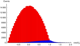
(a)

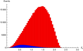
(b)

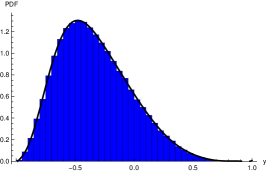
(c)

Figure 1: Histograms of $4\cdot 10^{5}$ pseudo events for the neutrino inclusive decay $B\to D\mu X_{\bar{\nu}}$ [figures (a) and (b)], as well as for the decay $B\to D\tau(\to\mu\nu\bar{\nu})\bar{\nu}$ [figure (c)]. We show histograms of distributions in the (misreconstructed) angle $\cos\vartheta_{\mu}$ [figure (a)], and $E_{\mu}$, the muon energy in the $\bar{B}$ rest frame [figure (b)]. The red areas correspond to the neutrino-inclusive decay, while the blue areas highlight the contributions stemming only from $B\to D\tau(\to\mu\nu\bar{\nu})\bar{\nu}$. We also show the histogram of $E_{\mu}\big{|}_{3\nu}$ and its compatibility with our ansatz eq. (35) [figure (c)].

Distribution in $\cos\vartheta_{[\mu]}$

In the neutrino inclusive decay, the misreconstructed observable $\cos\vartheta_{[\mu]}$ as given in eq. (13) is no longer bounded by $+1$. We find that it attains its maximal value

$$\max\cos\vartheta_{[\mu]}\big{|}_{3\nu}\simeq 56.7\qquad\text{for }q^{2}=(M_{B}-M_{D})^{2},\quad q_{[\nu_{\tau}\bar{\nu}_{\mu}]}^{2}=m_{\tau}^{2},\quad\cos\vartheta_{[\tau]}=-\cos\vartheta^{*}_{[\mu]}=1\,.$$ (30)

The distribution of $\cos\vartheta_{[\mu]}$ in the neutrino-inclusive decay is shown in figure 1(a), where we also disentangle the individual $1\nu$ and $3\nu$ contributions. We find that $\cos\vartheta_{[\mu]}$ exceeds $1$ for $\sim 23\%$ of the $3\nu$ events, and exceeds $2$ for $\sim 1.3\%$ of $3\nu$ events. As a consequence, we decide against a parametrization of the neutrino-inclusive PDF $P(\cos\vartheta_{\mu})$ in terms of Legendre polynomials (or any other orthonormal polynomial basis).

On the other hand, our findings imply that the $\cos\vartheta_{[\mu]}$ distribution can be used to extract the product $R_{D}\mathcal{B}(\tau\to\mu\bar{\nu}\nu)$ from data. We can indeed write

$$R_{D}\mathcal{B}(\tau\to\mu\bar{\nu}\nu)=\frac{\rho^{\rm exp}_{D}}{\rho_{D}^{0}-\rho^{\rm exp}_{D}}$$ (31)

where

$$\rho_{D}^{0}\equiv\frac{\#\text{of $3\nu$ events with }\cos\vartheta_{\mu}>1}{\text{total \# of $3\nu$ events}}\,,\qquad\rho^{\rm exp}_{D}\equiv\frac{\#\text{of $X_{\nu}$ events with }\cos\vartheta_{\mu}>1}{\text{total \# of $X_{\nu}$ events}}$$ (32)

Based on our MC pseudo events, we find

$$\rho^{0}_{D}=0.234\pm 0.001\,$$ (33)

where the error is dominantly statistical, and arises from our limited number of MC samples. We explicitly cross check our uncertainty estimate by re-running the simulations with modified inputs on the $B\to D$ form factors. We find that shifting any single individual constraint in table 1 by $1\sigma$ yields results that are compatible with the interval given in eq. (33).

The distribution in $E_{\mu}$

The distribution of $E_{\mu}$ in the neutrino-inclusive decay is shown in figure 1(b). We find that a lower cut $E_{\mu}>1.0\,$ can reduce the rate of of misidentified $3\nu$ events by a factor of $\sim 4$, while $\sim 76\%$ of the $1\nu$ events (the signal) remain. This corresponds to a reduction of the rate of background events in the neutrino-inclusive decay from its maximum value of $R_{D}\mathcal{B}(\tau\to\mu\nu\bar{\nu})\approx 5.2\%$ down to $1.3\%$.

Alternatively, one can subtract the $3\nu$ background from the neutrino-inclusive rate. For this purpose we proceed to obtain the relevant PDF of $3\nu$ events. Since the ranges of $E_{\mu}\Big{|}_{1\nu}$ and $E_{\mu}\Big{|}_{3\nu}$ are very similar, we can remap their union to a new kinematic variable $y$,

$$y\equiv\frac{2E_{\mu}}{E_{\mu}^{\text{max}}}-1\,,\qquad\text{with }E_{\mu}^{\text{max}}=\max\left(E_{\mu}\Big{|}_{1\nu},\,E_{\mu}\Big{|}_{3\nu}\right)\simeq 2.31\,\,,\qquad\text{so that }-1\leq y\leq+1\,.$$ (34)

We then make an ansatz for the PDF $P_{3}(y)\equiv{\mathrm{d}}\Gamma_{3}\,/{\mathrm{d}}y\,$ by expanding in Legendre polynomials $p_{k}(y)$:

$$P_{3}(y)=\frac{1}{2}+\sum_{k=1}^{12}c^{(3)}_{k}p_{k}(y)\,.$$ (35)

Since the Legendre polynomials form an orthogonal basis of function on the support $[-1,+1]$, the coefficients $c^{(3)}_{k}$ are independent of the degree of $P_{3}(y)$. Their mean values and covariance are obtained using the method of moments; see Beaujean et al. (2015) for a recent review. We find that our ansatz eq. (35) describes the PDF exceptionally well, and refer to figure 1(c) for the visualization. Our results for the mean values and covariance matrix of the moments are compiled in table 3. They can be used in upcoming experimental studies in order to cross check the signal/background discrimination.

III.2 $\bar{B}\to\pi\mu X_{\bar{\nu}}$

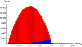
(a)

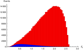
(b)

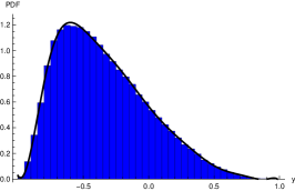
(c)

Figure 2: Histograms of $4\cdot 10^{5}$ pseudo events for the neutrino inclusive decay $B\to\pi\mu X_{\bar{\nu}}$ [figures (a) and (b)], as well as for the decay $B\to\pi\tau(\to\mu\nu\bar{\nu})\bar{\nu}$ [figure (c)]. We show histograms of distributions in the (misreconstructed) angle $\cos\vartheta_{\mu}$ [figure (a)], and $E_{\mu}$, the muon energy in the $\bar{B}$ rest frame [figure (b)]. The red areas correspond to the neutrino-inclusive decay, while the blue areas highlight the contributions stemming only from $B\to\pi\tau(\to\mu\nu\bar{\nu})\bar{\nu}$. We also show the histogram of $E_{\mu}\big{|}_{3\nu}$ and its compatibility with our ansatz eq. (35) [figure (c)].

Based on the $\bar{B}\to\pi$ form factors parameters as described in appendix A, we obtain

$$R_{\pi}^{\text{SM}}=0.70\pm 0.01\,,$$ (36)

which is in good visual agreement with the plot of $R_{\pi}$ in figure 8 of Ref. Khodjamirian et al. (2011). This result implies a potentially larger impact of the $3\nu$ decays as a background in the extraction of both $R_{\pi}$ and $|V_{ub}|$.

Distribution in $\cos\vartheta_{[\mu]}$

As in the case of $\bar{B}\to D\mu X_{\bar{\nu}}$, the misreconstructed observable $\cos\vartheta_{[\mu]}$ is no longer bounded from above by $+1$. However, we find that its maximal value is much smaller for $\bar{B}\to\pi$ transitions than it is for $\bar{B}\to D$ transitions:

$$\max\cos\vartheta_{[\mu]}\big{|}_{3\nu}\simeq 3.75\qquad\text{for }q^{2}=(M_{B}-M_{\pi})^{2},\quad q_{[\nu_{\tau}\bar{\nu}_{\mu}]}^{2}=m_{\tau}^{2},\quad\cos\vartheta_{[\tau]}=-\cos\vartheta^{*}_{[\mu]}=1\,.$$ (37)

A consequence of this smaller upper bound in $\bar{B}\to\pi$ transitions, the tail of $3\nu$ events is much lighter; see figure 2(a). This is also reflected in our numerical result for the ratio $\rho^{0}_{\pi}$,

$$\rho^{0}_{\pi}=(2.89\pm 0.03)\cdot 10^{-2}\,.$$ (38)

We can therefore not recommend to extract the ratio $R_{\pi}$ through a lower cut on $\cos\vartheta_{[\mu]}$. Our result also shows that more than $97\%$ of $3\nu$ events fall in the physical region of $1\nu$ events.

Distribution in $E_{\mu}$

We find that a lower cut $E_{\mu}>1.5\,$ can reduce the rate of of misidentified $3\nu$ events by a factor of $\sim 10$, while $\sim 69\%$ of the $1\nu$ events (the signal) remain. This corresponds to a reduction of the rate of background events in the neutrino-inclusive decay from its maximum value of $R_{\pi}\mathcal{B}(\tau\to\mu\nu\bar{\nu})\simeq 12.1\%$ down to $\sim 1.2\%$.

For the range of $E_{\mu}$ we find

$$\max\left(E_{\mu}\Big{|}_{1\nu}\,,E_{\mu}\Big{|}_{3\nu}\right)\simeq 2.64\,\,,$$ (39)

and the energy ranges are overlapping given our numerical precision. Thus, the description of the neutrino-inclusive rate though $E_{\mu}$, or equivalently $y$, should work even better for $\bar{B}\to\pi$ transitions than for $\bar{B}\to D$ transitions. Our results for the mean values and covariance matrix of the Legendre moments $c_{k}^{(3)}$ are compiled in table 4. We refer to figure 2(c) for a comparison of $P_{3}(y)$ with our MC pseudo events.

III.3 Implications for the extraction of $|V_{cb}|$ and $|V_{ub}|$

Using the above results we can finally draw some semi-quantitative conclusions about the error in the extraction $|V_{cb}|$ and $|V_{ub}|$ from $b\to c(u)\ell\nu$ decays. The presence of the $\tau\to\mu\bar{\nu}\nu$ background in those processes can be dealt with, experimentally, in different ways. The two extreme cases we can envisage are the following: i) reduction of the background via explicit cuts; ii) fully inclusive subtraction. The first method can be applied to exclusive decays such as those discussed in the present paper. As shown above, combining cuts in $E_{\mu}$ and $\cos\vartheta_{[\mu]}$ leads to a significant reduction of the $\tau\to\mu\bar{\nu}\nu$ contamination in $\bar{B}\to D\mu X_{\bar{\nu}}$, with negligible implications for the extraction of $|V_{cb}|$. However, this procedure cannot be applied to fully inclusive modes. In the latter case, the $\tau\to\mu\bar{\nu}\nu$ contamination is more likely to be simply subtracted from the total number of events. If this subtraction is made assuming the SM expectation of $R_{D}$ (and $R_{D*}$), it leads to systematic error if $\Delta R_{D}\not=0$, i.e. in presence of New Physics Greljo et al. (2015). The maximal value of this error is

$$\frac{\Delta|V_{cb}|^{(\rm incl.)}}{|V_{cb}|}=\frac{1}{2}\Delta R_{D}\mathcal{B}(\tau\to\mu\bar{\nu}\nu)\approx 0.9\%\,,$$ (40)

which is not far from the combined theory and experimental error presently quoted for $|V_{cb}|$ Olive et al. (2014). We thus conclude that the $\tau\to\mu\bar{\nu}\nu$ contamination must be carefully analyzed in the determination of $|V_{cb}|$.

The impact of the $\tau\to\mu\bar{\nu}\nu$ contamination is more difficult to be estimated in the $|V_{ub}|$ case. On the one hand, the large value of $R_{\pi}$ leads to a potentially larger impact. On the other hand, even in inclusive analyses some cut on $E_{\mu}$ is unavoidable in order to reduce the $b\to c\ell\nu$ background: as shown above, this naturally leads to a significant reduction of the $\tau\to\mu\bar{\nu}\nu$ contamination. Given the present large experimental errors, the $\tau\to\mu\bar{\nu}\nu$ contamination is likely to be a subleading correction in the extraction of $|V_{ub}|$, but it is certainly an effect that has to be properly analyzed in view of future high-statistics data.

IV Summary

Lepton Flavor Universality tests in charged-current semileptonic $B$ decays provide a very interesting window on possible physics beyond the SM. In the paper we have analyzed how the leptonic $\tau\to\mu\bar{\nu}\nu$ decays affect the determination of the LFU ratios $R_{P}$, where $P=D,\pi$. In particular, we have presented a complete analytical determination of the observable distributions (energy spectrum and helicity angle of the muon) of the $\bar{B}\to P\tau(\to\mu\bar{\nu}\nu)\bar{\nu}$ decay chain. This result has allowed us to identify clean strategies both to extract $R_{P}$ from measurements of the $\bar{B}\to P\mu X_{\bar{\nu}}$ neutrino-inclusive rate, and also to minimize the impact of the $\tau\to\mu\bar{\nu}\nu$ decay in the three-body $\bar{B}\to P\mu\nu$ modes. Finally, this study has also allowed us to conclude that the $b\to c\tau(\to\ell\bar{\nu}\nu)\nu$ background in $b\to c\ell\nu$ decays represents a non-negligible source of uncertainty for the extraction of $|V_{cb}|$ in presence of NP modifying $R_{D}$: its impact could reach the $\sim 1\%$ level and has to be analyzed with care mode by mode.

Appendix A $\bar{B}\to P$ form factors

	$f_{+}(0\,^{2})$	$f_{+}(4\,^{2})$	$f_{+}(8\,^{2})$	$f_{+}(t_{-})$	$f_{0}(4\,^{2})$	$f_{0}(8\,^{2})$	$f_{0}(t_{-})$
mean
	$0.665$	$0.798$	$0.972$	$1.177$	$0.729$	$0.810$	$0.901$
covariance matrix
$f_{+}(0\,^{2})$	$1.128\times 10^{-3}$	$1.042\times 10^{-3}$	$9.230\times 10^{-4}$	$7.727\times 10^{-4}$	$1.093\times 10^{-3}$	$1.063\times 10^{-3}$	$1.045\times 10^{-3}$
$f_{+}(4\,^{2})$	$1.042\times 10^{-3}$	$1.079\times 10^{-3}$	$1.108\times 10^{-3}$	$1.123\times 10^{-3}$	$1.026\times 10^{-3}$	$1.017\times 10^{-3}$	$1.021\times 10^{-3}$
$f_{+}(8\,^{2})$	$9.230\times 10^{-4}$	$1.108\times 10^{-3}$	$1.331\times 10^{-3}$	$1.576\times 10^{-3}$	$9.307\times 10^{-4}$	$9.511\times 10^{-4}$	$9.865\times 10^{-4}$
$f_{+}(t_{-})$	$7.727\times 10^{-4}$	$1.123\times 10^{-3}$	$1.576\times 10^{-3}$	$2.112\times 10^{-3}$	$8.108\times 10^{-4}$	$8.681\times 10^{-4}$	$9.425\times 10^{-4}$
$f_{0}(4\,^{2})$	$1.093\times 10^{-3}$	$1.026\times 10^{-3}$	$9.307\times 10^{-4}$	$8.108\times 10^{-4}$	$1.126\times 10^{-3}$	$1.165\times 10^{-3}$	$1.210\times 10^{-3}$
$f_{0}(8\,^{2})$	$1.063\times 10^{-3}$	$1.017\times 10^{-3}$	$9.511\times 10^{-4}$	$8.681\times 10^{-4}$	$1.165\times 10^{-3}$	$1.283\times 10^{-3}$	$1.410\times 10^{-3}$
$f_{0}(t_{-})$	$1.045\times 10^{-3}$	$1.021\times 10^{-3}$	$9.865\times 10^{-4}$	$9.425\times 10^{-4}$	$1.210\times 10^{-3}$	$1.410\times 10^{-3}$	$1.635\times 10^{-3}$

Table 1: Mean values and covariance matrix for the data points reconstructed from Na et al. (2015) at $q^{2}\in\{0\,^{2},4\,^{2},8\,^{2},t_{-}=(M_{B}^{2}-M_{D}^{2})\}$.

	$f_{+}(18\,^{2})$	$f_{+}(22\,^{2})$	$f_{+}(26\,^{2})$	$f_{0}(18\,^{2})$	$f_{0}(22\,^{2})$	$f_{0}(26\,^{2})$
mean
	$1.016$	$1.971$	$6.443$	$0.417$	$0.609$	$0.961$
covariance matrix
$f_{+}(18\,^{2})$	$3.492\times 10^{-3}$	$1.997\times 10^{-3}$	$1.648\times 10^{-3}$	$1.067\times 10^{-3}$	$2.904\times 10^{-4}$	$1.096\times 10^{-4}$
$f_{+}(22\,^{2})$	$1.997\times 10^{-3}$	$3.371\times 10^{-3}$	$6.193\times 10^{-3}$	$2.123\times 10^{-4}$	$2.167\times 10^{-4}$	$1.294\times 10^{-4}$
$f_{+}(26\,^{2})$	$1.648\times 10^{-3}$	$6.193\times 10^{-3}$	$7.419\times 10^{-2}$	$2.064\times 10^{-3}$	$1.139\times 10^{-3}$	$1.346\times 10^{-3}$
$f_{0}(18\,^{2})$	$1.067\times 10^{-3}$	$2.123\times 10^{-4}$	$2.064\times 10^{-3}$	$8.478\times 10^{-4}$	$4.266\times 10^{-4}$	$3.150\times 10^{-4}$
$f_{0}(22\,^{2})$	$2.904\times 10^{-4}$	$2.167\times 10^{-4}$	$1.139\times 10^{-3}$	$4.266\times 10^{-4}$	$3.923\times 10^{-4}$	$4.009\times 10^{-4}$
$f_{0}(26\,^{2})$	$1.096\times 10^{-4}$	$1.294\times 10^{-4}$	$1.346\times 10^{-3}$	$3.150\times 10^{-4}$	$4.009\times 10^{-4}$	$6.467\times 10^{-4}$

Table 2: Mean values and covariance matrix for the data points reconstructed from Bailey et al. (2015) at $q^{2}\in\{18\,^{2},22\,^{2},26\,^{2}\}$.

The hadronic matrix element for the vector current between two pseudoscalar states is commonly (e.g. Bourrely et al. (2009)) expressed in terms of two form factor

$$\bra{P(k)}\bar{c}\gamma^{\mu}b\ket{\bar{B}(p)}=f_{+}(q^{2})\left[(p+k)^{\mu}-\frac{M_{B}^{2}-M_{P}^{2}}{q^{2}}q^{\mu}\right]+f_{0}(q^{2})\frac{M_{B}^{2}-M_{P}^{2}}{q^{2}}q^{\mu}\,.$$ (41)

In the above, $q^{\mu}\equiv p^{\mu}-k^{\mu}$. In the limit $q^{2}\to 0$ one finds a relation between the two form factors in the form of

$$f_{+}(0)=f_{0}(0)\,,$$ (42)

otherwise eq. (41) would diverge.

While the heavy quark limit can be used as a guiding principle to parametrize both form factors, we prefer not to apply it. Instead, we follow the BCL ansatz Bourrely et al. (2009) and write

$$f_{+}(q^{2}) =\frac{f_{+}(0)}{1-q^{2}/M_{R(1^{-})}^{2}}\left[1+\sum_{k=1}^{3}\alpha^{+}_{k}z^{k}(q^{2};t_{+},0)\right]\,,$$ (43)

$$f_{0}(q^{2}) =\frac{f_{+}(0)}{1-q^{2}/M_{R(0^{+})}^{2}}\left[1+\sum_{k=1}^{2}\alpha^{0}_{k}z^{k}(q^{2},t_{+},0)\right]\,,$$

where $M_{R(1^{-})}$ and $M_{R(0^{+})}$ denote the masses of the low-lying resonances with spin/parity quantum numbers $J=1^{-}$ and $J=0^{+}$, respectively. Note the use of $f_{+}(0)$ in the parametrization of $f_{0}(q^{2})$, which automatically fulfills the equation of motion eq. (42). In the parametrization eq. (43), we make use of the conformal mapping from $q^{2}$ to $z$, where

$$z(q^{2};t_{+},t_{0})=\frac{\sqrt{t_{+}-q^{2}}-\sqrt{t_{+}-t_{0}^{\phantom{2}}}}{\sqrt{t_{+}-q^{2}}-\sqrt{t_{+}-t_{0}^{\phantom{2}}}}\,.$$ (44)

Following Bourrely et al. (2009) we impose $\operatorname{Im}{f_{+}(q^{2})}=(q^{2}-t_{+})^{3/2}$ close to the pair-production threshold $t_{+}\equiv(M_{B}+M_{D})^{2}$. This leads to a relation between the expansion parameters $\alpha^{+}_{k}$:

$$\alpha^{+}_{3}=\frac{1}{3}\sum_{k=1}^{K-1}(-1)^{k}k\,\alpha^{+}_{k}\,.$$ (45)

$\bar{B}\to D$

The lattice QCD results as presented in Na et al. (2015) follow the BCL parametrization, however, they do not automatically fulfill the equation of motion eq. (42). We therefore reconstruct lattice data points for four different choices of $q^{2}$ (see table 1), and fit our choice of the parametrization to these reconstructed points. We use $M_{R(1^{-})}=6.330$ and $M_{R(0^{+})}=6.420$ as in Na et al. (2015).

$\bar{B}\to\pi$

The lattice QCD results as presented in Bailey et al. (2015) follow the BCL parametrization. However, they do not automatically fulfill the equation of motion eq. (42). Moreover, for the form factor $f_{0}(q^{2})$, no pole for a low-lying resonance scalar resonance is used. We therefore reconstruct lattice data points for three different choices of $q^{2}$ in the domain for which lattice data point had been obtained (see table 2). In addition, we use the results of a recent Light-Cone Sum Rules (LCSR) study Sentitemsu Imsong et al. (2015) for the form factor $f_{+}$ at $q^{2}=\{0,10\}\,^{2}$. The LCSR results provide, beyond the form factor $f_{+}$, also its first and second derivatives with respect to $q^{2}$. We fit our choice of the parametrization to the aforementioned constraints. We use $M_{R(1^{-})}=5.325$ and $M_{R(0^{+})}=5.540$.

Appendix B Scalar Products

In order to facilitate the comparison with our results, we list here all scalar products that emerge in the calculation of eq. (22).

The scalar products involving $p$ are

$$p\cdot q =\frac{M_{B}^{2}+q^{2}-M_{D}^{2}}{2}\,,$$ (46)

$$p\cdot q_{[\tau]} =\frac{(1-\beta_{\tau})(M_{B}^{2}+q^{2}-M_{D}^{2})-\beta_{\tau}\sqrt{\lambda}\cos\vartheta_{[\tau]}}{2}$$ (47)

$$p\cdot q_{[\mu]} =\frac{1}{2}\beta_{\nu\bar{\nu}}\Big{[}(M_{B}^{2}+q^{2}-M_{D}^{2})((1-\beta_{\tau})+\beta_{\tau}\cos\vartheta^{*}_{[\mu]}$$ (48)

$$\quad-\sqrt{\lambda}(\beta_{\tau}+(1-\beta_{\tau})\cos\vartheta^{*}_{[\mu]})\cos\vartheta_{[\tau]}$$

$$\quad+\sqrt{\lambda}\sqrt{\frac{1}{2}-\beta_{\tau}}\sin\vartheta^{*}_{[\mu]}\sin\vartheta_{\tau}\cos\phi\Big{]}\,.$$

The scalar product involving $q$ read

$$q\cdot q_{[\tau]} =(1-\beta_{\tau})q^{2}\,,$$ (49)

$$q\cdot q_{[\mu]} =\beta_{\nu\bar{\nu}}((1-\beta_{\tau})+\beta_{\tau}\cos\vartheta^{*}_{[\mu]})q^{2}\,,$$ (50)

$$q\cdot q_{[\bar{\nu}_{\mu}]} =\frac{1}{2}\Big{[}(1-\beta_{\nu\bar{\nu}})(1-\beta_{\tau})-\beta_{\nu\bar{\nu}}(1-\beta_{\tau})\cos\vartheta^{**}_{[\bar{\nu}_{\mu}]}$$ (51)

$$\quad-\beta_{\tau}(\beta_{\nu\bar{\nu}}-(1-\beta_{\nu\bar{\nu}})\cos\vartheta^{**}_{[\bar{\nu}_{\mu}]})\cos\vartheta^{*}_{[\mu]}$$

$$\quad-2\sqrt{\frac{1}{2}-\beta_{\nu\bar{\nu}}}\beta_{\tau}\sin\vartheta^{*}_{[\mu]}\sin\vartheta^{**}_{[\bar{\nu}_{\mu}]}\cos\phi^{**}\Big{]}q^{2}\,.$$

For scalar products involving $q_{[\tau]}$ we find

$$q_{[\tau]}\cdot q_{[\mu]} =\beta_{\nu\bar{\nu}}q_{[\tau]}^{2}\,,$$ (52)

$$q_{[\tau]}\cdot q_{[\bar{\nu}_{\mu}]} =\frac{1}{2}\big{[}(1-\beta_{\nu\bar{\nu}})-\beta_{\nu\bar{\nu}}\cos\vartheta^{**}_{[\bar{\nu}_{\mu}]}\big{]}q_{[\tau]}^{2}\,.$$ (53)

For the antisymmetric tensors we obtain

$$\varepsilon(p,q,q_{[\mu]},q_{[\bar{\nu}_{\mu}]}) =\frac{\beta_{\nu\bar{\nu}}\beta_{\tau}\sqrt{\frac{1}{2}-\beta_{\tau}}}{2}\sqrt{\lambda}q^{2}\sin\vartheta^{*}_{[\mu]}\sin\vartheta_{[\tau]}\sin\phi\,,$$ (54)

In all of the above, we abbreviate

$$\beta_{\tau} =\frac{q^{2}+q_{[\tau]}^{2}}{2q^{2}}\,, \beta_{\nu\bar{\nu}} =\frac{q_{[\tau]}^{2}+q_{[\nu_{\tau}\bar{\nu}_{\mu}]}^{2}}{2q_{[\tau]}^{2}}\,.$$ (55)

Appendix C Results for the Legendre Ansatz in $P_{3}(y)$

The mean values and covariance matrices for the Legendre moments in the PDFs $P_{3}(y)$ of $\bar{B}\to D\tau(\to\mu\bar{\nu}\nu)\bar{\nu}$ and $\bar{B}\to\pi\tau(\to\mu\bar{\nu}\nu)\bar{\nu}$ decays are listed in tables 3 and 4, respectively.

$c_{k}$	$-5.02\times 10^{-1}$	$-4.82\times 10^{-1}$	$7.41\times 10^{-1}$	$-1.98\times 10^{-1}$	$-1.71\times 10^{-1}$	$1.85\times 10^{-1}$	$-9.99\times 10^{-2}$	$1.99\times 10^{-2}$	$2.67\times 10^{-2}$	$-3.22\times 10^{-2}$	$1.45\times 10^{-2}$	$2.46\times 10^{-3}$
$k$	$1$	$2$	$3$	$4$	$5$	$6$	$7$	$8$	$9$	$10$	$11$	$12$
1	$5.22\times 10^{-7}$	$-6.69\times 10^{-7}$	$-4.86\times 10^{-7}$	$1.05\times 10^{-6}$	$-3.07\times 10^{-7}$	$-2.92\times 10^{-7}$	$2.84\times 10^{-7}$	$-1.28\times 10^{-7}$	$1.54\times 10^{-8}$	$3.84\times 10^{-8}$	$-4.05\times 10^{-8}$	$1.27\times 10^{-8}$
2	$-6.69\times 10^{-7}$	$1.33\times 10^{-6}$	$-7.86\times 10^{-8}$	$-1.75\times 10^{-6}$	$1.52\times 10^{-6}$	$-5.29\times 10^{-9}$	$-6.93\times 10^{-7}$	$4.86\times 10^{-7}$	$-1.59\times 10^{-7}$	$-3.22\times 10^{-8}$	$8.67\times 10^{-8}$	$-5.88\times 10^{-8}$
3	$-4.86\times 10^{-7}$	$-7.86\times 10^{-8}$	$1.94\times 10^{-6}$	$-1.11\times 10^{-6}$	$-1.74\times 10^{-6}$	$2.05\times 10^{-6}$	$-2.31\times 10^{-7}$	$-7.24\times 10^{-7}$	$5.56\times 10^{-7}$	$-2.21\times 10^{-7}$	$3.3\times 10^{-9}$	$8.87\times 10^{-8}$
4	$1.05\times 10^{-6}$	$-1.75\times 10^{-6}$	$-1.11\times 10^{-6}$	$4.09\times 10^{-6}$	$-1.78\times 10^{-6}$	$-2.56\times 10^{-6}$	$2.89\times 10^{-6}$	$-4.67\times 10^{-7}$	$-8.47\times 10^{-7}$	$7.25\times 10^{-7}$	$-3.16\times 10^{-7}$	$2.88\times 10^{-8}$
5	$-3.07\times 10^{-7}$	$1.52\times 10^{-6}$	$-1.74\times 10^{-6}$	$-1.78\times 10^{-6}$	$4.94\times 10^{-6}$	$-1.94\times 10^{-6}$	$-3.15\times 10^{-6}$	$3.43\times 10^{-6}$	$-5.29\times 10^{-7}$	$-9.97\times 10^{-7}$	$8.51\times 10^{-7}$	$-3.7\times 10^{-7}$
6	$-2.92\times 10^{-7}$	$-5.29\times 10^{-9}$	$2.05\times 10^{-6}$	$-2.56\times 10^{-6}$	$-1.94\times 10^{-6}$	$5.89\times 10^{-6}$	$-2.37\times 10^{-6}$	$-3.58\times 10^{-6}$	$3.93\times 10^{-6}$	$-6.18\times 10^{-7}$	$-1.12\times 10^{-6}$	$9.4\times 10^{-7}$
7	$2.84\times 10^{-7}$	$-6.93\times 10^{-7}$	$-2.31\times 10^{-7}$	$2.89\times 10^{-6}$	$-3.15\times 10^{-6}$	$-2.37\times 10^{-6}$	$6.9\times 10^{-6}$	$-2.75\times 10^{-6}$	$-4.06\times 10^{-6}$	$4.45\times 10^{-6}$	$-7.26\times 10^{-7}$	$-1.23\times 10^{-6}$
8	$-1.28\times 10^{-7}$	$4.86\times 10^{-7}$	$-7.24\times 10^{-7}$	$-4.67\times 10^{-7}$	$3.43\times 10^{-6}$	$-3.58\times 10^{-6}$	$-2.75\times 10^{-6}$	$7.84\times 10^{-6}$	$-3.1\times 10^{-6}$	$-4.57\times 10^{-6}$	$4.97\times 10^{-6}$	$-8.\times 10^{-7}$
9	$1.54\times 10^{-8}$	$-1.59\times 10^{-7}$	$5.56\times 10^{-7}$	$-8.47\times 10^{-7}$	$-5.29\times 10^{-7}$	$3.93\times 10^{-6}$	$-4.06\times 10^{-6}$	$-3.1\times 10^{-6}$	$8.75\times 10^{-6}$	$-3.44\times 10^{-6}$	$-5.04\times 10^{-6}$	$5.46\times 10^{-6}$
0	$3.84\times 10^{-8}$	$-3.22\times 10^{-8}$	$-2.21\times 10^{-7}$	$7.25\times 10^{-7}$	$-9.97\times 10^{-7}$	$-6.18\times 10^{-7}$	$4.45\times 10^{-6}$	$-4.57\times 10^{-6}$	$-3.44\times 10^{-6}$	$9.68\times 10^{-6}$	$-3.81\times 10^{-6}$	$-5.51\times 10^{-6}$
11	$-4.05\times 10^{-8}$	$8.67\times 10^{-8}$	$3.3\times 10^{-9}$	$-3.16\times 10^{-7}$	$8.51\times 10^{-7}$	$-1.12\times 10^{-6}$	$-7.26\times 10^{-7}$	$4.97\times 10^{-6}$	$-5.04\times 10^{-6}$	$-3.81\times 10^{-6}$	$1.06\times 10^{-5}$	$-4.14\times 10^{-6}$
12	$1.27\times 10^{-8}$	$-5.88\times 10^{-8}$	$8.87\times 10^{-8}$	$2.88\times 10^{-8}$	$-3.7\times 10^{-7}$	$9.4\times 10^{-7}$	$-1.23\times 10^{-6}$	$-8.\times 10^{-7}$	$5.46\times 10^{-6}$	$-5.51\times 10^{-6}$	$-4.14\times 10^{-6}$	$1.15\times 10^{-5}$

Table 3: Mean values and covariance matrix for the Legendre moments $c^{(3)}_{k}$ in the parametrization of the PDF $P_{3}(y)$ in the Decay $\bar{B}\to D\tau(\to\mu\bar{\nu}\nu)\bar{\nu}$. We use $k\leq 12$.

$c_{k}$	$-5.2\times 10^{-1}$	$-3.6\times 10^{-1}$	$6.14\times 10^{-1}$	$-3.02\times 10^{-1}$	$6.0\times 10^{-2}$	$6.47\times 10^{-2}$	$-1.18\times 10^{-1}$	$1.09\times 10^{-1}$	$-6.88\times 10^{-2}$	$2.31\times 10^{-2}$	$1.11\times 10^{-2}$	$-3.\times 10^{-2}$
$k$	$1$	$2$	$3$	$4$	$5$	$6$	$7$	$8$	$9$	$10$	$11$	$12$
1	$6.58\times 10^{-7}$	$-7.83\times 10^{-7}$	$-5.16\times 10^{-7}$	$1.03\times 10^{-6}$	$-4.39\times 10^{-7}$	$-4.1\times 10^{-12}$	$1.7\times 10^{-7}$	$-2.17\times 10^{-7}$	$1.69\times 10^{-7}$	$-8.57\times 10^{-8}$	$5.91\times 10^{-9}$	$3.7\times 10^{-8}$
2	$-7.83\times 10^{-7}$	$1.62\times 10^{-6}$	$-2.61\times 10^{-7}$	$-1.79\times 10^{-6}$	$1.74\times 10^{-6}$	$-4.72\times 10^{-7}$	$-2.72\times 10^{-7}$	$4.94\times 10^{-7}$	$-4.59\times 10^{-7}$	$2.78\times 10^{-7}$	$-8.51\times 10^{-8}$	$-6.28\times 10^{-8}$
3	$5.16\times 10^{-7}$	$-2.61\times 10^{-7}$	$2.24\times 10^{-6}$	$-1.04\times 10^{-6}$	$-1.83\times 10^{-6}$	$2.\times 10^{-6}$	$-5.54\times 10^{-7}$	$-2.55\times 10^{-7}$	$4.78\times 10^{-7}$	$-4.5\times 10^{-7}$	$2.7\times 10^{-7}$	$-7.25\times 10^{-8}$
4	$1.03\times 10^{-6}$	$-1.79\times 10^{-6}$	$-1.04\times 10^{-6}$	$4.14\times 10^{-6}$	$-1.93\times 10^{-6}$	$-2.14\times 10^{-6}$	$2.58\times 10^{-6}$	$-9.36\times 10^{-7}$	$-6.37\times 10^{-8}$	$4.21\times 10^{-7}$	$-4.79\times 10^{-7}$	$3.73\times 10^{-7}$
5	$-4.39\times 10^{-7}$	$1.74\times 10^{-6}$	$-1.83\times 10^{-6}$	$-1.93\times 10^{-6}$	$5.3\times 10^{-6}$	$-2.28\times 10^{-6}$	$-2.71\times 10^{-6}$	$3.21\times 10^{-6}$	$-1.22\times 10^{-6}$	$-9.6\times 10^{-9}$	$5.19\times 10^{-7}$	$-6.59\times 10^{-7}$
6	$-4.1\times 10^{-12}$	$-4.72\times 10^{-7}$	$2.\times 10^{-6}$	$-2.14\times 10^{-6}$	$-2.28\times 10^{-6}$	$6.14\times 10^{-6}$	$-2.55\times 10^{-6}$	$-3.21\times 10^{-6}$	$3.72\times 10^{-6}$	$-1.35\times 10^{-6}$	$-1.12\times 10^{-7}$	$6.54\times 10^{-7}$
7	$1.7\times 10^{-7}$	$-2.72\times 10^{-7}$	$-5.54\times 10^{-7}$	$2.58\times 10^{-6}$	$-2.71\times 10^{-6}$	$-2.55\times 10^{-6}$	$7.03\times 10^{-6}$	$-2.91\times 10^{-6}$	$-3.57\times 10^{-6}$	$4.09\times 10^{-6}$	$-1.45\times 10^{-6}$	$-1.11\times 10^{-7}$
8	$-2.17\times 10^{-7}$	$4.94\times 10^{-7}$	$-2.55\times 10^{-7}$	$-9.36\times 10^{-7}$	$3.21\times 10^{-6}$	$-3.21\times 10^{-6}$	$-2.91\times 10^{-6}$	$8.05\times 10^{-6}$	$-3.41\times 10^{-6}$	$-3.92\times 10^{-6}$	$4.56\times 10^{-6}$	$-1.68\times 10^{-6}$
9	$1.69\times 10^{-7}$	$-4.59\times 10^{-7}$	$4.78\times 10^{-7}$	$-6.37\times 10^{-8}$	$-1.22\times 10^{-6}$	$3.72\times 10^{-6}$	$-3.57\times 10^{-6}$	$-3.41\times 10^{-6}$	$9.09\times 10^{-6}$	$-3.79\times 10^{-6}$	$-4.39\times 10^{-6}$	$5.1\times 10^{-6}$
10	$-8.57\times 10^{-8}$	$2.78\times 10^{-7}$	$-4.5\times 10^{-7}$	$4.21\times 10^{-7}$	$-9.6\times 10^{-9}$	$-1.35\times 10^{-6}$	$4.09\times 10^{-6}$	$-3.92\times 10^{-6}$	$-3.79\times 10^{-6}$	$9.99\times 10^{-6}$	$-4.11\times 10^{-6}$	$-4.83\times 10^{-6}$
11	$5.91\times 10^{-9}$	$-8.51\times 10^{-8}$	$2.7\times 10^{-7}$	$-4.79\times 10^{-7}$	$5.19\times 10^{-7}$	$-1.12\times 10^{-7}$	$-1.45\times 10^{-6}$	$4.56\times 10^{-6}$	$-4.39\times 10^{-6}$	$-4.11\times 10^{-6}$	$1.09\times 10^{-5}$	$-4.5\times 10^{-6}$
12	$3.7\times 10^{-8}$	$-6.28\times 10^{-8}$	$-7.25\times 10^{-8}$	$3.73\times 10^{-7}$	$-6.59\times 10^{-7}$	$6.54\times 10^{-7}$	$-1.11\times 10^{-7}$	$-1.68\times 10^{-6}$	$5.1\times 10^{-6}$	$-4.83\times 10^{-6}$	$-4.5\times 10^{-6}$	$1.19\times 10^{-5}$

Table 4: Mean values and covariance matrix for the Legendre moments $c^{(3)}_{k}$ in the parametrization of the PDF $P_{3}(y)$ in the Decay $\bar{B}\to\pi\tau(\to\mu\bar{\nu}\nu)\bar{\nu}$. We use $k\leq 12$.

References

- Cabibbo (1963) N. Cabibbo, Meeting of the Italian School of Physics and Weak Interactions Bologna, Italy, April 26-28, 1984, Phys. Rev. Lett. 10, 531 (1963), [,648(1963)].
- Kobayashi and Maskawa (1973) M. Kobayashi and T. Maskawa, Prog. Theor. Phys. 49, 652 (1973).
- Kowalewski and Mannel (2014) R. Kowalewski and T. Mannel, in Review of Particle Physics (RPP), Vol. C38 (2014) p. 090001.
- Bailey et al. (2015) J. A. Bailey et al. (Fermilab Lattice, MILC), Phys. Rev. D92, 014024 (2015), arXiv:1503.07839 [hep-lat] .
- Na et al. (2015) H. Na, C. M. Bouchard, G. P. Lepage, C. Monahan, and J. Shigemitsu (HPQCD), Phys. Rev. D92, 054510 (2015), arXiv:1505.03925 [hep-lat] .
- Lees et al. (2013) J. P. Lees et al. (BaBar), Phys. Rev. D88, 072012 (2013), arXiv:1303.0571 [hep-ex] .
- Huschle et al. (2015) M. Huschle et al. (Belle), Phys. Rev. D92, 072014 (2015), arXiv:1507.03233 [hep-ex] .
- Hamer et al. (2015) P. Hamer et al. (Belle), (2015), arXiv:1509.06521 [hep-ex] .
- Aaij et al. (2015) R. Aaij et al. (LHCb), Phys. Rev. Lett. 115, 111803 (2015), [Addendum: Phys. Rev. Lett.115,no.15,159901(2015)], arXiv:1506.08614 [hep-ex] .
- Celis et al. (2013) A. Celis, M. Jung, X.-Q. Li, and A. Pich, JHEP 01, 054 (2013), arXiv:1210.8443 [hep-ph] .
- Alonso et al. (2015) R. Alonso, B. Grinstein, and J. M. Camalich, JHEP 10, 184 (2015), arXiv:1505.05164 [hep-ph] .
- Greljo et al. (2015) A. Greljo, G. Isidori, and D. Marzocca, JHEP 07, 142 (2015), arXiv:1506.01705 [hep-ph] .
- Calibbi et al. (2015) L. Calibbi, A. Crivellin, and T. Ota, Phys. Rev. Lett. 115, 181801 (2015), arXiv:1506.02661 [hep-ph] .
- Olive et al. (2014) K. A. Olive et al. (Particle Data Group), Chin. Phys. C38, 090001 (2014).
- Dutta et al. (2013) R. Dutta, A. Bhol, and A. K. Giri, Phys. Rev. D88, 114023 (2013), arXiv:1307.6653 [hep-ph] .
- Becirevic et al. (2016) D. Becirevic, S. Fajfer, I. Nisandzic, and A. Tayduganov, (2016), arXiv:1602.03030 [hep-ph] .
- van Dyk et al. (2016) D. van Dyk et al., (2016), 10.5281/zenodo.50968.
- Bourrely et al. (2009) C. Bourrely, I. Caprini, and L. Lellouch, Phys. Rev. D79, 013008 (2009), [Erratum: Phys. Rev.D82,099902(2010)], arXiv:0807.2722 [hep-ph] .
- Sentitemsu Imsong et al. (2015) I. Sentitemsu Imsong, A. Khodjamirian, T. Mannel, and D. van Dyk, JHEP 02, 126 (2015), arXiv:1409.7816 [hep-ph] .
- Metropolis et al. (1953) N. Metropolis, A. W. Rosenbluth, M. N. Rosenbluth, A. H. Teller, and E. Teller, J. Chem. Phys. 21, 1087 (1953).
- Hastings (1970) W. K. Hastings, Biometrika 57, 97 (1970).
- Bordone et al. (2016) M. Bordone, G. Isidori, and D. van Dyk, (2016), 10.5281/zenodo.50843.
- Beaujean et al. (2015) F. Beaujean, M. Chrząszcz, N. Serra, and D. van Dyk, Phys. Rev. D91, 114012 (2015), arXiv:1503.04100 [hep-ex] .
- Khodjamirian et al. (2011) A. Khodjamirian, T. Mannel, N. Offen, and Y. M. Wang, Phys. Rev. D83, 094031 (2011), arXiv:1103.2655 [hep-ph] .