Solvability of the non-linear Dirichlet problem with Integro-Differential operators

Abstract

This paper analyzes the solvability of a class of elliptic non-linear Dirichlet problems with jumps. The contribution of the paper is the construction of the supersolution required in Perron’s method. This is achieved by solving the exit time problem of an Itô jump diffusion. The proof of this relies on the proof of continuity of the entrance time and point with respect to the Skorohod topology.

60H30, 47G20, 93E20, 60J75, 49L25, 35J60, 35J66

1 Introduction

Problem setup

Consider an equation of the form

(1.1) $$F(u,x)+u(x)-\ell(x)=0,\ x\in O$$

with the boundary value

(1.2) $$u(x)=g(x),\ x\in O^{c}.$$

Here

$$F(u,x)=-\inf_{a\in[\underline{a},\overline{a}]}H(u,x,a)-\mathcal{I}(u,x)$$

where $\underline{a}\leq\overline{a}$ are given two real numbers and

(1.3) $$\mathcal{I}(u,x)=\int_{\mathbb{R}^{d}}(u(x+y)-u(x)-Du(x)\cdot yI_{B_{1}}(y))\nu(dy),$$

$$H(u,x,a)=\frac{1}{2}tr(A(a)D^{2}u(x))+b(a)\cdot Du(x),$$

with $A(a)=\sigma^{\prime}(a)\sigma(a)$, and $\nu(\cdot)$ is a Lévy measure on $\mathbb{R}^{d}$, i.e. $\int_{\mathbb{R}^{d}}(1\wedge|y|^{2})\nu(dy)<\infty$. Here, $B_{r}(x)$ is a ball of radius $r$ with center $x$, and we denote $B_{r}(0)$ by $B_{r}$ for simplicity. To simplify our presentation, we will use the following additional set of assumptions throughout the paper.

Assumption 1.1.

1. $O$ is a connected open bounded set in $\mathbb{R}^{d}$.

2. $\sigma,b\in C^{0,1}(\mathbb{R})$; $\ell,g\in C_{0}(\mathbb{R}^{d})$.

3. $\nu(dy)=\hat{\nu}(y)dy$ is a Lévy measure satisfying $\hat{\nu}\in C_{0}(\mathbb{R}^{d}\setminus\{0\})$.

For some $\alpha\in(0,2)$, if $\nu$ is given by

$$\nu(dy)=\frac{dy}{|y|^{d+\alpha}},$$

then $\nu$ satisfies Assumption 1.1, and the integral operator is denoted by $\mathcal{I}(u,x)=-(-\Delta)^{\alpha/2}u(x)$ as convention. For convenience, we write $-(-\Delta)^{0}u=0$.

Literature review and a motivating example

A function $u$ is said to be a solution of Dirichlet problem (1.1)-(1.2), if $u\in C(\bar{O})$ satisfies (1.1) in the viscosity sense in $O$ and $u=g$ on $O^{c}$. It is worth to note that, as far as Dirichlet problem (1.1)-(1.2) concerned, one can generalize the boundary condition (1.2) by

(1.4) $$\max\{F(u,x)+u(x)-\ell(x),u-g\}\geq 0\geq\min\{F(u,x)+u(x)-\ell(x),u-g\}\hbox{ on }O^{c}$$

without loss of uniqueness in the viscosity sense.

In contrast to the (classical) Dirichlet problem (1.1)-(1.2), Dirichlet problem (1.1)-(1.4) is referred to a generalized Dirichlet problem. For the generalized Dirichlet problem without nonlocal operator, there were many excellent discussions on the solvability with the comparison principle and Perron’s method, see for instance, [6], [7], [3], and Section 7 of [16]. Also see [19] and [11] for an analysis of this using the dynamic programming principle. Recently, the solvability result has been extended to nonlinear equations associated to Integro-differential operators, see [5], [4], [1], [25], and the references therein.

Compared to the generalized Dirichlet problem, there are relatively less discussions available on the classical Dirichlet problem associated with the Integral operators in the aforementioned references. The following example motivates our analysis:

Example 1.1.

Determine the existence and uniqueness of the viscosity solution for the Dirichlet problem given by,

(1.5) $$|\partial_{x_{1}}u|+(-\Delta)^{\alpha/2}u+u-1=0,\ \forall x\in O=(-1,1)\times(-1,1),$$

where $\alpha\in[0,2]$, with the boundary condition

$$u(x)=0,\ \forall x\in O^{c}.$$

This problem is only partially resolved in the existing literature:

• If $\alpha=0$, there is no solution. In fact, one can directly check that $u(x)=1-e^{-1+|x_{1}|}$ is the unique solution of the generalized Dirichlet problem, but not a solution of classical Dirichlet problem due to its loss of boundary at $\{(x_{1},x_{2}):|x_{2}|=1,|x_{1}|<1\}$.

• If $\alpha\in[1,2]$, there is a unique solution by [4].

• If $\alpha\in(0,1)$, although there is unique solution of generalized Dirichlet problem by [25], it was not known whether this solution solves the classical Dirichlet problem. Our main result Theorem 2.1 demonstrates that this in fact is the case, see Example 2.4. It is also pointed out there that existence and uniqueness still holds for all $\alpha\in(0,2]$ as long as the boundary satisfies exterior cone condition, which itself is a new result.

1.1 Work outline

This work focuses on the sufficient condition of the existence and uniqueness of the viscosity solution for Dirichlet problem of (1.1)-(1.2).

One alternative in proving this result is using the stochastic Perron methodology introduced by [8, 10, 9], and [13] for the application of this approach to a particular exit time problem. With this methodology one can in fact identify the value function of the exit time control problem with the generalized Dirichlet problem (1.1)-(1.4) using a similar analysis to the proofs of Theorems 2 and 3 in [22]. Then as in [19] (also see [11]), if we can a priori show that the value function is continuous (this can fail at the boundary), we can conclude that the value function also solves the classical Dirichlet problem (1.1)-(1.2).

Since either one needs to prove continuity separately or has to impose a stronger version of the comparison principle as in Theorem 1 of [22], we will not pursue the stochastic Perron approach here. We will instead approach this problem using the classical Perron method. Using the idea of constructing a supersolution satisfying the boundary conditions from an auxiliary stochastic exit time problem as in [12] (and in [13] in a slightly different set-up), we will be able to apply [5] and obtain a unique viscosity solution. This result, which is the main contribution of the paper, is presented in Theorem 2.1.

The technical step of the proof of Theorem 2.1 involves proving the continuity of the value function of the exit time problem of an Itô jump diffusion, see Proposition 2.4. In general, due to the non-local property, continuity of the value function up to a stopping time is much more delicate than the counterpart of the purely differential form. We establish this result by investigating the continuity set of the of entrance time and entrance point mappings with respect to the Skorohod topology; see Theorems 3.2 and 3.4. Then we show that these sets have full measure under our assumption in the proof of Proposition 2.4. It is easy to show that the continuous sample paths are a subset of the points of lower semi-continuity of the entrance time to a closed interval, see e.g. [17]. However, the continuity set is difficult to identify. In fact, continuity does not hold in general for the entrance time as shown in Appendix C (see Example C.3) or Page 657 of [24]. Moreover, Example C.4 demonstrates that the situation for the continuity of the entrance point mapping is even worse. Our contribution here is the identification of the discontinuity set as a null set under our assumption about the geometry of the boundary.

2 Existence of a unique solution for the Dirichlet problem

2.1 Two different definitions of viscosity properties

In this section, we give two different definitions of viscosity properties, Definition 2.1 and Definition 2.2 respectively. Definition 2.1 involves only with $C^{2}$ smooth test functions, which will be used later to verify the supersolution property of a certain value function associated to some exit control problem. Compared to Definition 2.1, Definition 2.2 is given with more test functions including non-smooth functions, and it’s much harder to be used directly in this paper to verify viscosity solution property. However, Definition 2.2 of this paper is exactly Definition 2 of [5], where it was used to provide the proof of comparison principle and Perron’s method. In this connection, we shall prove the equivalence of Definition 2.2 and Definition 2.1.

Definition 2.1 below is consistent to the Definition 1 of [5], which will be used to establish the existence of the solution in this paper. To proceed, for a function $u:\bar{O}\mapsto\mathbb{R}$, we define its extension by

$$u^{g}=(uI_{\bar{O}}+gI_{\bar{O}^{c}})^{*},\quad u_{g}=(uI_{\bar{O}}+gI_{\bar{O}^{c}})_{*},$$

where $f^{*}$ and $f_{*}$ stand for USC (upper semicontinuous) and LSC (Lower semicontinuous) envelopes of the function $f$, respectively. We also define the supertest function space, for $u\in USC$ and $x\in\mathbb{R}^{d}$

(2.1) $$J^{+}(u,x)=\{\phi\in C_{b}^{\infty}(\mathbb{R}^{d}),\hbox{ such that }\phi\geq u^{g}\hbox{ and }\phi(x)=u(x)\}.$$

Analogously, the subtest function space is given by, for $u\in LSC$ and $x\in\mathbb{R}^{d}$

(2.2) $$J^{-}(u,x)=\{\phi\in C_{b}^{\infty}(\mathbb{R}^{d}),\hbox{ such that }\phi\leq u_{g}\hbox{ and }\phi(x)=u(x)\}.$$

Definition 2.1.

1. We say a function $u\in USC(\bar{O})$ satisfies the viscosity subsolution property at $x\in O$, if the following inequality holds,

   (2.3) $$F(\phi,x)+u(x)-\ell(x)\leq 0,\ \forall\phi\in J^{+}(u,x).$$

2. We say a function $u\in LSC(\bar{O})$ satisfies the viscosity supersolution property at $x\in O$, if the following inequality holds,

   (2.4) $$F(\phi,x)+u(x)-\ell(x)\geq 0,\ \forall\phi\in J^{-}(u,x).$$

Next, we observe that $\phi\mapsto F(\phi,x)$ of (2.3) and (2.4) could be well defined for a function being $C^{\infty}$-smooth only at some neighborhood of $x$. Indeed, for an arbitrary $x\in\mathbb{R}^{d}$, if we define a function space $C_{x}$ by

(2.5) $$C_{x}=\{\phi:\exists\hat{r}>0,\ \phi_{1}\in C^{\infty},\ \phi_{2}\in L^{1},\hbox{ s.t. }\phi=\phi_{1}I_{\bar{B}_{\hat{r}}(x)}+\phi_{2}(1-I_{\bar{B}_{\hat{r}}(x)})\},$$

one can directly verify that $\phi\mapsto\mathcal{I}(\phi,x)$ is well defined for $\phi\in C_{x}$, with a property

(2.6) $$\mathcal{I}(\phi,x)=b_{r}\cdot D\phi(x)+\mathcal{I}_{r,1}(\phi,x)+\mathcal{I}_{r,2}(\phi,x),\ \forall r>0$$

where

1. $b_{r}=\int_{B_{1}\setminus B_{r}}y\nu(dy).$

2. $\mathcal{I}_{r,1}(\phi,x)=\int_{B_{r}}(\phi(x+y)-\phi(x)-D\phi(x)\cdot y)\nu(dy)$

3. $\mathcal{I}_{r,2}(\phi,x)=\int_{\mathbb{R}\setminus B_{r}}(\phi(x+y)-\phi(x))\nu(dy)$.

In the above, $\int_{B_{1}\setminus B_{r}}$ for $r>1$ is understood as $-\int_{B_{r}\setminus B_{1}}$. Note that, (a) the identity (2.6) agrees with the original definition (1.3) of $\mathcal{I}$; (b) $r$ in (2.6) could be larger than $\hat{r}$ of (2.5). This observation allows us to use more test functions from $C^{\infty}$ to $C_{x}$ compared to Definition 2.1. In this below, Definition 2.2 is consistent to Definition 2 of [5].

Definition 2.2.

1. We say a function $u\in USC(\bar{O})$ satisfies the viscosity subsolution property at $x\in O$, if for all $\phi\in C_{x}$ with (1) $\phi(x)=u(x)$; (2) $\phi-u\geq 0$ on $\bar{O}$, satisfies

   (2.7) $$-b_{r}\cdot D\phi(x)-\mathcal{I}_{r,1}(\phi,x)-\mathcal{I}_{r,2}(u^{g},x)-\inf_{a\in[\underline{a},\overline{a}]}H(\phi,x,a)+u(x)-\ell(x)\leq 0,\ \forall r>0,$$

2. We say a function $u\in LSC(\bar{O})$ satisfies the viscosity supersolution property at $x\in O$, if for all $\phi\in C_{x}$ with (1) $\phi(x)=u(x)$; (2) $\phi-u\leq 0$ on $\bar{O}$

   (2.8) $$-b_{r}\cdot D\phi(x)-\mathcal{I}_{r,1}(\phi,x)-\mathcal{I}_{r,2}(u_{g},x)-\inf_{a\in[\underline{a},\overline{a}]}H(\phi,x,a)+u(x)-\ell(x)\geq 0,\ \forall r>0.$$

Proposition 2.1.

Definition 2.1 is equivalent to Definition 2.2.

The proof is relegated to Appendix  A.

2.2 Perron’s method

Definition 2.3.

A function $u\in USC(\bar{O})$ (resp. $u\in LSC(\bar{O})$) is said to be a viscosity subsolution (resp. supersolution) of (1.1) - (1.2), if $u$ satisfies the subsolution (resp. supersolution) property at each $x\in O$ and $u=g$ at $O^{c}$. A function $u\in C(\bar{O})$ is said to be a solution of (1.1) - (1.2), if it is a sub and supersolution of (1.1) - (1.2) at the same time.

Proposition 2.2 (Comparison Principle).

If $u$ and $v$ are subsolution and supersolution of (1.1) - (1.2), then $u\leq v$.

Proof.

Since Definition 2.1 is in fact equivalent to Definition 2 of [5] by Proposition 2.1, the statement above follows from the corresponding statement in Theorem 3 of [5].

Proposition 2.3 (Perron’s Method).

If there exist a subsolution $\underline{u}$ and a supersolution $\overline{u}$ to (1.1) - (1.2), then

$$w(x)=\inf\{u\in LSC(\bar{O}):u\hbox{ is subsolution}\}$$

is the unique solution in $C(\bar{O})$.

We relegate the proof of Proposition 2.3 in Appendix B.

Remark 2.1.

According to Propositions 2.2 and 2.3, the remaining task is to show the existence of a subsolution $\underline{u}$ and a supersolution $\overline{u}$. In general, as far as the classical Dirichlet boundary concerned, one shall not expect the existence of subsolution and supersolution for free due to Example 7.8 of [16]. In this regard, some sufficient conditions of the existence of subsolution and supersolution of Dirichlet problem is provided by Example 4.6 of [16], and the general case has remained open. In this paper, we address the issue of constructing a supersolution, which we carry out in the next subsection.

2.3 Stochastic exit control problem for an Itô jump diffusion

To proceed, we consider an exit control problem with Markovian policy. We consider a fixed filtered probability space $(\Omega,\mathcal{F},\mathbb{P},\{\mathcal{F}_{t},t>0\})$, on which $W$ is a standard Brownian motion and $L$ is a Lévy process with generating triplet $(0,\nu,0)$, see notions of Lévy process in [23] or [14]. We consider a stochastic differential equation controlled by a Lipschitz continuous function $m:\mathbb{R}^{d}\mapsto[\underline{a},\overline{a}]$,

(2.9) $$X_{t}=x+\int_{0}^{t}b(m(X_{s}))dt+\int_{0}^{t}\sigma(m(X_{s}))dW_{s}+L_{t},$$

By [2], (2.9) admits a unique solution which has a càdlàg version, and we assume $X$ to be a càdlàg process. Next, we define the first exit times

(2.10) $$\tau=\inf\{t>0,X_{t}\notin O\}$$

and

(2.11) $$\hat{\tau}=\inf\{t>0,X_{t}\notin\bar{O}\}.$$

Let $\mathbb{D}^{d}_{\infty}$ be the space of càdlàg functions on $[0,\infty)$ with Skorohod metric given by $d^{o}_{\infty}$, see detailed definition in Section C. We are interested in the following subset of Markovian policy space $\mathcal{M}$ defined by

(2.12) $$\mathcal{M}=\{m\in C^{0,1}(\mathbb{R}^{d},[\underline{a},\overline{a}]):\mathbb{P}^{m,x}(\hat{\tau}=0)=1,\ \forall x\in\partial O\}.$$

For a given $(x,m)\in\mathbb{R}^{d}\times\mathcal{M}$, we use $\mathbb{P}^{m,x}$ to denote the probability measure on $\mathbb{D}^{d}_{\infty}$ induced by $X_{t}$, i.e. $\mathbb{P}^{m,x}(B)=\mathbb{P}(X\in B)$ for all Borel set $B$ of $(\mathbb{D}^{d}_{\infty},d^{o}_{\infty})$ . We also use $\mathbb{E}^{m,x}$ to denote the expectation operator with respect to $\mathbb{P}^{m,x}$.

Proposition 2.4.

Let $m\in\mathcal{M}$ of (2.12), and

$$V_{m}(x):=\mathbb{E}^{m,x}\big{[}\int_{0}^{\tau}e^{-s}\ell(X_{s})ds+g(X_{\tau})\big{]}$$

with $\tau$ given by (2.10). Then, the function $V_{m}$ belongs to $C(\bar{O})$.

Proof.

This result is a corollary of the technical results presented in Theorems 3.2 and 3.4. See Section 3.1.

2.4 Main result

We next state the main result of this paper, which is a corollary of Proposition 2.4.

Theorem 2.1.

If $\mathcal{M}\neq\emptyset$ and $u=g$ is a subsolution of (1.1) - (1.2), then there exists a unique continuous viscosity solution of (1.1) - (1.2).

Remark 2.2.

The sufficient condition in Theorem 2.1 requires some regularity of the boundary with respect to some controlled process, this requirement is not that strong. For example, the regularity in Example 4.6 of [16] and [3] asks the boundary to be $C^{2}$. We can in fact consider non-smooth boundaries satisfying exterior cone condition with some appropriate Integro-differential operators, see the first paragraph of Example 2.4, for instance.

Proof of Theorem 2.1. The uniqueness holds by Proposition 2.2, and we shall prove the existence by Perron’s method Proposition 2.3. To proceed, we shall find out sub and supersolution. Note that $g$ is a subsolution and below we will show that $V_{m}$ is a supersolution for any $m\in\mathcal{M}$.

We fix a policy $m\in\mathcal{M}$. By Proposition 2.4, we have $V_{m}\in C(\bar{O})$ with $V_{m}(x)=g(x)$ for all $x\in\partial O$. So, it’s enough to show that $V_{m}$ satisfies the supersolution property in $O$, i.e.

$$F_{m}(\phi,x)+\phi(x)-\ell(x)\geq 0,\ \forall x\in O,\phi\in J^{-}(V_{m},x).$$

where $F_{m}(\phi,x)=-H(\phi,x,m(x))-\mathcal{I}(\phi,x)$. To the contrary, let’s assume

$$F_{m}(\phi,x)+\phi(x)-\ell(x)=-\epsilon<0$$

for some $x\in O$ and $\phi\in J^{-}(V_{m},x)$. By Lemma A.8 and the continuity of $m$, the function $F_{m}(\phi,\cdot)$ is continuous at $x$, and there exists $h>0$ that

(2.13) $$\sup_{|y-x|<h}F_{m}(\phi,y)+\phi(y)-\ell(y)<-\epsilon/2.$$

Since $X$ of (2.9) is a càdlàg process, the first exit time satisfies $\mathbb{P}^{m,x}\{\tau>0\}=1$. By the strong Markov property of the process $X$, we rewrite the value function $V_{m}$ as, for any stopping time $\theta\in(0,\tau]$

$$V_{m}(x)=\mathbb{E}^{m,x}\Big{[}e^{-\theta}V_{m}(X_{\theta})+\int_{0}^{\theta}e^{-s}\ell(X_{s})ds\Big{]},$$

which in turn implies that, with the fact of $\phi\in J^{-}(V_{m},x)$

$$\phi(x)\geq\mathbb{E}^{m,x}\Big{[}e^{-\theta}\phi(X_{\theta})+\int_{0}^{\theta}e^{-s}\ell(X_{s})ds\Big{]},$$

On the other hand, one can use Dynkin’s formula on $\phi$ to write

$$\mathbb{E}^{m,x}[e^{-\theta}\phi(X_{\theta})]=\phi(x)-\mathbb{E}^{m,x}\Big{[}\int_{0}^{\theta}e^{-s}(F_{m}(\phi,X_{s})+\phi(X_{s}))ds\Big{]}.$$

By adding up the above two formulas together, it yields that

$$\mathbb{E}^{m,x}\Big{[}\int_{0}^{\theta}e^{-s}(F_{m}(\phi,X_{s})+\phi(X_{s})-\ell(X_{s}))ds\Big{]}\geq 0.$$

Finally we take $\theta=\inf\{t>0:X(t)\notin B_{h}(x)\}\wedge\tau$ in the above and note that $\theta>0$ almost surely in $\mathbb{P}^{m,x}$. This leads to a contradiction to (2.13). $\square$

Remark 2.3.

The sufficient condition of Theorem 2.1 consists of (1) $\mathcal{M}\neq\emptyset$; and (2) subsolution property $g$ to ensure the uniqueness and existence of the solution. We will give two examples. In the first example we will address the open problem we posed in Example  1.1 (the condition that $\mathcal{M}\neq\emptyset$ is satisfied). In the second example, we will address the necessity of the assumption on $g$.

Example 2.4 (Resolution of the open problem in Example  1.1).

Consider the set-up in Example 1.1 with $\alpha\in(0,2)$. We address the existence and uniqueness problem we proposed below. We should point out that our proof would not be affected if the domain $O$ is replaced by any open connected set satisfying exterior cone condition.

We first rewrite the equation (1.5) as

$$-\inf_{a\in[-1,1]}\{a\ \partial_{x_{1}}u\}+(-\Delta)^{\alpha/2}u+u-1=0\ \hbox{ on }O.$$

For $m\in\mathcal{M}$, we set

$$X_{t}=x+\int_{0}^{t}m(X_{s})e_{1}ds+L_{t}^{\alpha}$$

where $e_{1}=(1,0)^{\prime}$ is a unit vector and $L^{\alpha}$ is a symmetric $\alpha$-stable process with the generating triplet $(0,\nu(dy)=\frac{dy}{|y|^{d+\alpha}},0)$. The corresponding value function is

$$V_{m}(x)=\mathbb{E}^{m,x}\Big{[}\int_{0}^{\tau}e^{-s}ds\Big{]}=\mathbb{E}^{m,x}[1-e^{-\tau}]$$

with the first exit time $\tau=\inf\{t>0,X_{t}\notin O\}$. One can directly check both conditions required by Theorem 2.1:

• If $\alpha>0$, then we take $m(x)=0$ and corresponding $X$ is given by

  $$X_{t}=x+L_{t}^{\alpha};$$

  In this case, $\mathbb{P}^{m,x}\{\hat{\tau}=0\}=1$ for all $x\in\partial O$ and $\mathcal{M}\neq\emptyset$.

• $u=0$ is subsolution.

$\square$

Example 2.5 (On the necessity of the subsolution property of $g$).

In terms of subsolution property of $g$ in Dirichlet problem, the boundary data $g$ shall be understood as any USC function $\bar{g}$ with $\bar{g}=g$ outside of the domain. This condition indeed a relaxation of the condition V.2.11 of [19].

One can check $u(x)=1-e^{-1+|x|}$ is the unique solution of

$$|u^{\prime}|+u-1=0,\ \forall x\in(-1,1)\hbox{ with }u(\pm 1)=0.$$

However, there is no solution for

$$|u^{\prime}|+u+1=0,\ \forall x\in(-1,1)\hbox{ with }u(\pm 1)=0.$$

Indeed, if there were a solution $u$, the boundary condition $u(1)=0$ implies that $|u^{\prime}|+u+1>1/2$ in some neighborhood of $1$ due to the continuity of $u$, which leads to a contradiction. One can see that this equation does not satisfy the second condition, i.e. $u=0$ is not subsolution. $\square$

3 Continuity of Entrance time and point

In this section we will prove Proposition 2.4, which is the main ingredient of our main result. This result itself depends on two technical results, Theorems 3.2 and 3.4, which we consider as important technical contributions. First we will introduce some notations to state these results and motivate them. The proofs of these two results are lengthy. Therefore, after stating these results, we will first prove Proposition 2.4 (see Section 3.1) as a corollary and then return to proving Theorems 3.2 and 3.4 in Section 3.2.

We denote by $(\mathbb{D}^{d}_{t},d^{o}_{t})$ the complete space of càdlàg functions on $[0,t)$ taking values in $\mathbb{R}^{d}$ with Skorohod metric $d^{o}_{t}$, and by $(\mathbb{D}^{d}_{\infty},d^{o}_{\infty})$ the space of càdlàg functions on $[0,\infty)$. Since there is variance definitions on the Skorohod metric in the literature, we provide the explicit definition of Skorohod metric adopted by this paper in Appendix C taken from [15].

We also define the entrance time operator $T_{A}:\mathbb{D}^{d}_{\infty}\mapsto\mathbb{R}$ by, for a set $A\in\mathbb{R}^{d}$ and $a\in(0,\infty)$

(3.1) $$T_{A}(\omega)=\inf\{t\geq 0:\omega(t)\in A\},\ T_{A}^{a}(\omega)=\inf\{t\geq 0:\omega(t)\in A\}\wedge a,$$

By convention, $T_{A}(\omega)=\infty$ if $\omega(t)\notin A$ for all $t\geq 0$. Given a set $O$, we will call $T_{O^{c}}(\omega)$ as the exit time of $\omega$ from the set $O$.

As in [15] let $\Pi:\mathbb{D}^{d}_{\infty}\times[0,\infty)\mapsto\mathbb{R}^{d}$ defined by $\Pi(\omega,t)=\omega(t)$. Similarly, define the value at the first entrance point by

(3.2) $$\Pi_{O}(\omega)=\omega(T_{O^{c}}(\omega)).$$

Our goal is to investigate the sufficient condition such that the mappings $T_{O^{c}}$ and $\Pi_{O}$ are continuous for a given set $O$, and this will serve as an important tool for the existence of the solution.

Remark 3.1.

Example C.3 shows that $T_{O^{c}}$ is neither upper semicontinuous nor lower semicontinuous in general. Moreover, Example C.4 demonstrates that the situation for the continuity of $\Pi_{O}$ is even worse than the mapping $T_{O^{c}}$.

The following theorems are the main results of this section on the continuity of the two mappings $T_{O^{c}}$ and $\Pi_{O}$, and their proofs will be relegated to Section 3.2.3 and 3.2.4. Roughly speaking, both $T_{O^{c}}$ and $\Pi_{O}$ are continuous at $\omega$ if, at the first exit time

1. either $\omega$ exits from $O$ to $\bar{O}$ continuously by crossing $\partial O$;

2. or $\omega$ jumps from a point of $O$ to another point of $\bar{O}^{c}$.

Theorem 3.2.

$T_{O^{c}}$ is continuous w.r.t. Skorohod metric at any $\omega\in\Gamma_{O}$ where

(3.3) $$\Gamma_{O}:=\{\omega\in\mathbb{D}^{d}_{\infty}:T_{O^{c}}(\omega^{-})=T_{O^{c}}(\omega)=T_{\bar{O}^{c}}(\omega)\}.$$

Here

$$\omega^{-}(t)=\lim_{s\to t-}\omega(s),\ \forall\omega\in\mathbb{D}^{d}_{\infty}.$$

Remark 3.3.

It is worth noting that $\Gamma_{O}$ is not a superset of the continuous sample paths, since the second inequality in its definition may not be satisfied. So the lower semi-continuity side of the proof does not follow from the result in [17], which shows that the continuous sample paths to be in the points of lower semi-continuity of the above map.

Theorem 3.4.

$\Pi_{O}$ is continuous w.r.t. Skorohod metric at any $\omega\in\hat{\Gamma}_{O}$

(3.4) $$\hat{\Gamma}_{O}:=\{\omega\in\Gamma_{O}:\hbox{ if }\Pi_{O}(\omega^{-})\in\partial O,\hbox{ then }\Pi_{O}(\omega^{-})=\Pi_{O}(\omega)\}$$

3.1 Proof of Proposition 2.4

Let us denote $b_{m}=b\circ m$ and $\sigma_{m}=\sigma\circ m$.

If $x\in\partial O$, then $\tau=0$ $\mathbb{P}^{m,x}$-almost surely by definition and $V_{m}(x)=g(x)$. In the rest of the proof, let $x_{n}\to x\in\bar{O}$, and we will show the continuity of $V_{m}$ at $x$.

Step 1. In this step, we will show $\mathbb{P}^{m,x}(\hat{\Gamma}_{O})=1$ for all $x\in\bar{O}$ and $\hat{\Gamma}_{O}$ defined by (3.4). Since both $b_{m}$ and $\sigma_{m}$ are Lipschitz continuous, there exists unique strong solution $X$, which is càdlàg process with strong Markovian property, see Example 6.4.7 of [2]. Therefore, $m\in\mathcal{M}$ implies

(3.5) $$\mathbb{P}^{m,x}\{\tau=\hat{\tau}\}=1,\ \forall x\in\bar{O}.$$

Hence, for all $x\in\partial O$, we have $\Gamma_{O}=\hat{\Gamma}_{O}$ and $\mathbb{P}^{m,x}(\hat{\Gamma}_{O})=1$. Now, it remains to show $\mathbb{P}^{m,x}(\hat{\Gamma}_{O})=1,\ \forall x\in O.$ Let $x\in O$ and $\bar{\tau}=T_{O^{c}}(X^{-})$. We define

$$\bar{\tau}_{A}=\left\{\begin{array}[]{ll}\bar{\tau}&\hbox{ if }\omega\in A;\\ \infty&\hbox{ otherwise }\end{array}\right.\hbox{ and }\bar{\tau}_{B}=\left\{\begin{array}[]{ll}\bar{\tau}&\hbox{ if }\omega\in B;\\ \infty&\hbox{ otherwise. }\end{array}\right.$$

where

$$A=\{X^{-}(\bar{\tau})\in\partial O\}\hbox{ and }B=\{X^{-}(\bar{\tau})\neq X(\bar{\tau})\}.$$

The left continuity of $X^{-}$ implies $A\in\mathcal{F}_{\bar{\tau}-}$ and the hitting time $\bar{\tau}_{A}$ is a predictable stopping time, while $\bar{\tau}_{B}$ is totally inaccessible stopping time due to the jump by Meyer’s theorem, see Theorem III.4 of [21]. Therefore, we conclude $\mathbb{P}^{m,x}(\bar{\tau}_{A}=\bar{\tau}_{B})=0$ by Theorem III.3 of [21], and further we have $\mathbb{P}^{m,x}(A\cap B)=0$. Therefore, $X$ is continuous at $\bar{\tau}$ almost surely in $\mathbb{P}^{m,x}$. Together with (3.5), we conclude $\mathbb{P}^{m,x}(\hat{\Gamma}_{O})=1$.

Step 2. Recall that $\hat{\Gamma}_{O}$ and $\Pi_{O}$ are defined by (3.4) and (3.2), respectively. We will show that $f_{1},f_{2}$ are continuous at all $\omega\in\hat{\Gamma}_{O}$, where

$$f_{1}(\omega)=\int_{0}^{T_{O^{c}}(\omega)}e^{-s}\ell(\omega_{s})ds,\ \hbox{ and }\ f_{2}(\omega)=e^{-T_{O^{c}}(\omega)}g(\Pi_{O}(\omega)),\ \forall\omega\in\mathbb{D}^{d}_{\infty}.$$

The continuity of $f_{2}$ is the direct consequence of Theorem 3.2 and Theorem 3.4. So, it remains to show the continuity of $f_{1}$.

Suppose $\omega^{n}\to\omega\in\hat{\Gamma}_{O}$ in Skorohod metric, and we denote $T_{n}=T_{O^{c}}(\omega^{n})$ and $T=T_{O^{c}}(\omega)$, we conclude $f_{1}(\omega^{n})\to f_{1}(\omega)$ as $n\to\infty$, since

1. $T_{n}\to T$ due to Theorem 3.2;

2. $\omega^{n}\to\omega$ in $\mathbb{D}^{d}_{\infty}$ means that $\omega^{n}(s)\to\omega(s)$ for all $s\in D_{\omega}^{c}$, where $D_{\omega}^{c}$ is the complement of the countable set

   $$D_{\omega}:=\{s\in(0,\infty):\omega\hbox{ is discontinuous at }s\}.$$

   Together with the continuity of $\ell$, we have $\ell(\omega^{n}(s))\to\ell(\omega(s))$ almost everywhere on $(0,t)$ w.r.t. Lebesgue measure.

3. Finally, we have, as $n\to\infty$

   $$|f_{1}(\omega^{n})-f_{1}(\omega)|\leq\int_{0}^{T_{n}}e^{-qs}|\ell(\omega^{n}(s))-\ell(\omega(s))|ds+2K|T_{n}-T|\to 0.$$

Step 3. In this final step we will show that $V_{m}(x_{n})\to V_{m}(x)$ if $x_{n}\to x\in\bar{O}$. We first conclude $\mathbb{P}^{m,x_{n}}$ is weakly convergent to $\mathbb{P}^{m,x}$, since

1. By Theorem 3.2 of [20], $X$ satisfies

   $$\mathbb{E}\Big{[}\sup_{0\leq s\leq t}|X_{s}^{m,x_{n}}-X_{s}^{m,x}|^{2}\Big{]}\leq K_{t}|x_{n}-x|^{2}\to 0,\hbox{ as }n\to\infty.$$

   This means $\{X^{m,x_{n}}_{s}:0\leq s\leq t\}$ is convergent to $\{X_{s}^{m,x}:0\leq s\leq t\}$ $\mathbb{P}$-almost surely with respect to $L^{\infty}$, and hence convergent in distribution with respect to Skorohod metric. Weak convergence on any finite time interval implies the weak convergence on the entire time interval by Theorem 16.7 of [15].

Moreover, in the above two steps, we established $f_{1}+f_{2}$ is continuous $\mathbb{P}^{m,x}$-almost surely. Then, we apply the continuous mapping theorem and bounded convergence theorem to obtain

$$V_{m}(x_{n})=\mathbb{E}^{m,x_{n}}[(f_{1}+f_{2})(X)]\to\mathbb{E}^{m,x}[(f_{1}+f_{2})(X)]=V_{m}(x).$$

$\square$

3.2 Proofs of Theorems 3.2 and 3.4

3.2.1 Sufficiency of working in simpler topologies

Let $\Lambda_{\infty}$ be the set of continuous and strictly increasing maps of $[0,\infty)$ to itself. Let

$$\|\omega\|_{m}=\sup_{0\leq t\leq m}|\omega(t)|,\ \|\omega\|=\sup_{0\leq t<\infty}|\omega(t)|.$$

The topology induced by the above supnorm is finer than Skorohod topology. Therefore, the continuity of $\Pi_{O}$ at $\omega$ with respect to Skorohod topology automatically implies the continuity with respect to uniform topology. In this below, we will prove that the converse is also true: the continuity with respect to uniform topology implies the continuity of $\Pi_{O}$ with respect to Skorohod topology. This enables us to simplify our subsequent analysis by working on a series of simpler metrics.

Lemma 3.5.

$T_{O^{c}}(\omega\circ\lambda)=\lambda^{-1}\circ T_{O^{c}}(\omega)$ for all $\omega\in\mathbb{D}^{d}_{\infty}$ and $\lambda\in\Lambda_{\infty}$.

Proof 3.6.

$T_{O^{c}}(\omega\circ\lambda)=\inf\{t>0:\omega\circ\lambda(t)\notin O\}=\lambda^{-1}(\inf\{\lambda(t)>0:\omega(\lambda(t))\notin O\})=\lambda^{-1}\circ T_{O^{c}}(\omega).$

Lemma 3.7.

1. If $T_{O^{c}}^{m}$ is lower semicontinuous w.r.t $\|\cdot\|_{m}$ for all integer $m$, then $T_{O^{c}}$ is lower semicontinuous w.r.t $d_{\infty}^{o}$.

2. If $T_{O^{c}}^{m}$ is upper semicontinuous w.r.t $\|\cdot\|_{m}$ for all integer $m$, then $T_{O^{c}}$ is upper semicontinuous w.r.t $d_{\infty}^{o}$.

Proof 3.8.

We assume $T_{O^{c}}(\omega)\in(0,\infty)$, otherwise it’s obvious. Let $\lim_{n}d^{o}_{\infty}(\omega_{n},\omega)=0.$ By Theorem 16.1 of [15], there exists $\lambda_{n}\in\Lambda_{\infty}$ such that

$$\lim_{n}\|\lambda_{n}-1\|=0$$

and

$$\lim_{n}\|\omega_{n}\circ\lambda_{n}-\omega\|_{m}=0,\ \forall m\in\mathbb{N}.$$

1. We suppose $T_{O^{c}}^{m}$ is lower semicontinuous w.r.t. $\|\cdot\|_{m}$ for every integer $m$. Then, we have

   $$\lim\inf_{n}T_{O^{c}}^{m}(\omega_{n}\circ\lambda_{n})\geq T_{O^{c}}^{m}(\omega).$$

   Also, we have by Lemma 3.5

   $$|T_{O^{c}}^{m}(\omega_{n})-T_{O^{c}}^{m}(\omega_{n}\circ\lambda_{n})|=|T_{O^{c}}(\omega_{n})\wedge m-\lambda_{n}^{-1}\circ T_{O^{c}}(\omega_{n})\wedge m|\leq\|1-\lambda_{n}^{-1}\|\to 0.$$

   Thus, we have

   $$\lim\inf_{n}T_{O^{c}}^{m}(\omega_{n})\geq T_{O^{c}}^{m}(\omega).$$

   Therefore, for a big enough $m$ such that $m>T_{O^{c}}(\omega)$ holds, we have

   $$\lim\inf_{n}T_{O^{c}}(\omega_{n})\geq\lim\inf_{n}T_{O^{c}}^{m}(\omega_{n})\geq T_{O^{c}}^{m}(\omega)=T_{O^{c}}(\omega).$$

   This implies $T_{O^{c}}$ is also lower semicontinuous w.r.t. $d_{\infty}^{o}$.

2. We suppose $T_{O^{c}}^{m}$ is upper semicontinuous w.r.t. $\|\cdot\|_{m}$ for every integer $m$. Then, we have

   $$\lim\sup_{n}T_{O^{c}}^{m}(\omega_{n}\circ\lambda_{n})\leq T_{O^{c}}^{m}(\omega).$$

   Also, we have similarly $|T_{O^{c}}^{m}(\omega_{n})-T_{O^{c}}^{m}(\omega_{n}\circ\lambda_{n})|\to 0$ as $n\to\infty$ by Lemma 3.5, and conclude

   $$\lim\sup_{n}T_{O^{c}}^{m}(\omega_{n})\leq T_{O^{c}}^{m}(\omega)\leq T_{O^{c}}(\omega)\quad\hbox{ for all integer }m.$$

   Now we fix an integer $m>T_{O^{c}}(\omega)+1$. This means, $\forall\epsilon\in(0,1)$, there exists $N_{\epsilon}$ such that

   $$T_{O^{c}}(\omega_{n})\wedge m\leq T_{O^{c}}(\omega)+\epsilon,\quad\forall n\geq N_{\epsilon}.$$

   Since $m>T_{O^{c}}(\omega)+\epsilon$, the left hand side $T_{O^{c}}(\omega_{n})\wedge m$ must be equal to $T_{O^{c}}(\omega_{n})$, i.e.

   $$T_{O^{c}}(\omega_{n})\leq T_{O^{c}}(\omega)+\epsilon,\quad\forall n\geq N_{\epsilon}.$$

   This implies $T_{O^{c}}$ is also upper semicontinuous w.r.t. $d_{\infty}^{o}$.

3.2.2 The problem in dimension one

In this below, we will identify the continuity set in one dimensional càdlàg space for the mapping $T_{O^{c}}$ with respect to uniform topology induced by supnorm.

Lemma 3.9.

The mapping $\omega\mapsto T_{(-\infty,0)}^{m}(\omega)$ is upper semicontinuous in $\mathbb{D}^{1}_{\infty}$ w.r.t. $\|\cdot\|_{m}$ for every $m\in\mathbb{N}$.

Proof 3.10.

For convenience, we denote $\hat{T}_{m}(\omega)=T_{(-\infty,0)}(\omega)\wedge m$. It’s enough to show that

If $\|\omega_{n}-\omega\|_{m}\to 0$, then $\lim\sup_{n}\hat{T}_{m}(\omega_{n})\leq\hat{T}_{m}(\omega)$.

We prove it in two cases separately:

1. Assume $\inf_{0\leq t\leq m}\omega(t)>0$. This implies $\hat{T}_{m}(\omega)=m$. Given $\|\omega_{n}-\omega\|_{m}\to 0$, there exists $N$, such that

   $$\forall n>N,\ \|\omega_{n}-\omega\|_{m}<\frac{1}{2}\inf_{0\leq t\leq m}\omega(t).$$

   This yields

   $$\forall n>N,\ \forall s\in[0,m],\ \omega_{n}(s)-\omega(s)>-\frac{1}{2}\inf_{0\leq t\leq m}\omega(t).$$

   Therefore,

   $$\forall n>N,\ \forall s\in[0,m],\ \omega_{n}(s)>0,$$

   or equivalently, $\hat{T}_{m}(\omega_{n})=m$ for all $n>N$. This proves the conclusion of the first case.

2. Assume $\inf_{0\leq t\leq m}\omega(t)\leq 0$. Fix arbitrary $\epsilon>0$, then

   $$\exists t_{\epsilon}\in[\hat{T}_{m}(\omega),\hat{T}_{m}(\omega)+\epsilon)\hbox{ such that }\omega(t_{\epsilon})<0.$$

   Given $\|\omega_{n}-\omega\|_{m}\to 0$,

   $$\exists N\ \hbox{ such that }\ \|\omega_{n}-\omega\|_{m}<\frac{1}{2}|\omega(t_{\epsilon})|,\ \forall n\geq N.$$

   In particular, one can write $\omega_{n}(t_{\epsilon})-\omega(t_{\epsilon})<-\frac{1}{2}\omega(t_{\epsilon})$, or equivalently

   $$\exists N\hbox{ such that }\ \omega_{n}(t_{\epsilon})<0,\ \forall n\geq N.$$

   Therefore, $\hat{T}_{m}(\omega_{n})\leq t_{\epsilon}\leq\hat{T}_{m}(\omega)+\epsilon$ for all $n\geq N$. By taking $\lim\sup_{n}$ both sides, we have

   $$\lim\sup_{n}\hat{T}_{m}(\omega_{n})\leq\hat{T}_{m}(\omega)+\epsilon$$

   and the conclusion follows due to the arbitrary selection of $\epsilon$.

Lemma 3.11.

$\omega\mapsto T_{(-\infty,0]}^{m}(\omega_{*})$ is lower semicontinuous in $\mathbb{D}^{1}_{\infty}$ w.r.t. $\|\cdot\|_{m}$ for every $m\in\mathbb{N}$, where

$$\omega_{*}(t)=\lim\inf_{s\to t}\omega(s),\ \forall t>0$$

is the lower envelope of $\omega$.

Proof 3.12.

For simplicity, we denote

$$\tilde{T}_{m}(\omega)=T_{(-\infty,0]}(\omega_{*})\wedge m\hbox{ and }M[\omega](t)=\inf_{0\leq s\leq t}\omega(s).$$

Note that $M[\omega]=M[\omega_{*}]$ is a non-increasing process. It’s enough to show that

If $\|\omega_{n}-\omega\|_{m}\to 0$, then $\lim\inf_{n}\tilde{T}_{m}(\omega_{n})\geq\tilde{T}_{m}(\omega)$.

1. Assume $\tilde{T}_{m}(\omega)=m$. This implies $M[\omega](m)=M[\omega_{*}](m)>0$, otherwise $\tilde{T}_{m}(\omega)<m$. Given $\|\omega_{n}-\omega\|_{m}\to 0$,

   $$\exists N,\hbox{ such that }\|\omega_{n}-\omega\|_{m}<\frac{1}{2}M[\omega](m),\ \forall n\geq N,$$

   which implies, there exists $N$ such that

   $$\omega_{n}(t)>\omega(t)-\frac{1}{2}M[\omega](m)\geq\frac{1}{2}M[\omega](m)>0,\ \forall t\in(0,m),\ \forall n\geq N.$$

   Hence, $\tilde{T}_{m}(\omega_{n})=m$ for all $n\geq N$, and this proves the continuity at $\omega$ for this case.

2. Assume $\tilde{T}_{m}(\omega)<m$. Since $\omega_{*}$ is lower semicontinuous , we have

   $$M[\omega](\tilde{T}_{m}(\omega))\leq 0,\hbox{ and }M[\omega](t)>0,\forall t<\tilde{T}_{m}(\omega).$$

   Fix arbitrary $\epsilon>0$. Then, we have $M[\omega](\tilde{T}_{m}(\omega)-\epsilon)>0$, and

   $$\exists N,\hbox{ such that }\|\omega_{n}-\omega\|_{m}<\frac{1}{2}M[\omega](\tilde{T}_{m}(\omega)-\epsilon),\ \forall n\geq N.$$

   This leads to, for all $n\geq N$ and $t<\tilde{T}_{m}(\omega)-\epsilon$

   $$\omega_{n}(t)>\omega(t)-\frac{1}{2}M[\omega](\tilde{T}_{m}(\omega)-\epsilon)\geq\frac{1}{2}M[\omega](\tilde{T}_{m}(\omega)-\epsilon)>0.$$

   In other words, we have $\tilde{T}_{m}(\omega_{n})\geq\tilde{T}_{m}(\omega)-\epsilon$ for all $n\geq N$. So we conclude $\lim\inf_{n}\tilde{T}_{m}(\omega_{n})\geq\tilde{T}_{m}(\omega)$ for the this case.

Lemma 3.13.

1. $T_{(-\infty,0]}^{m}$ is upper semicontinuous on

   $$\{\omega\in\mathbb{D}^{1}_{\infty}:T_{(-\infty,0]}^{m}(\omega)=T_{(-\infty,0)}^{m}(\omega)\}\hbox{ w.r.t. }\|\cdot\|_{m};$$

2. $T_{(-\infty,0]}^{m}$ is lower semicontinuous on

   $$\{\omega\in\mathbb{D}^{1}_{\infty}:T_{(-\infty,0]}^{m}(\omega)=T_{(-\infty,0]}^{m}(\omega_{*})\}\hbox{ w.r.t. }\|\cdot\|_{m}.$$

Proof 3.14.

If (a) $\omega_{n}\to\omega$ w.r.t. $\|\cdot\|_{m}$; and (b) $T_{(-\infty,0]}^{m}(\omega)=T_{(-\infty,0)}^{m}(\omega)$, then Lemma 3.9 implies

$$\lim_{n}\sup T^{m}_{(-\infty,0]}(\omega_{n})\leq\lim_{n}\sup T^{m}_{(-\infty,0)}(\omega_{n})\leq T^{m}_{(-\infty,0)}(\omega)=T^{m}_{(-\infty,0]}(\omega),$$

which asserts the upper semicontinuity.

Similarly, if (a) $\omega_{n}\to\omega$ w.r.t. $\|\cdot\|_{m}$; and (b) $T_{(-\infty,0]}^{m}(\omega)=T_{(-\infty,0]}^{m}(\omega_{*})$, then Lemma 3.11 implies

$$\lim_{n}\inf T^{m}_{(-\infty,0]}(\omega_{n})\geq\lim_{n}\inf T^{m}_{(-\infty,0]}(\omega_{n,*})\geq T^{m}_{(-\infty,0]}(\omega_{*})=T^{m}_{(-\infty,0]}(\omega),$$

which asserts the lower semicontinuity.

3.2.3 Proof of Theorem 3.2

Step 1. The proof relies on a dimension reduction. Let us define the signed distance function

(3.6) $$\rho(x)=\left\{\begin{array}[]{ll}dist(x,\partial O)&\hbox{ if }x\in O;\\ -dist(x,\partial O)&\hbox{ otherwise}\end{array}\right.$$

Note that, if $O$ is open, then

$$T_{O^{c}}(\omega)=\inf\{t\geq 0:\omega(t)\notin O\}=\inf\{t\geq 0:\rho\circ\omega(t)\leq 0\}=T_{(-\infty,0]}(\rho\circ\omega),$$

and

$$T_{\bar{O}^{c}}(\omega)=\inf\{t\geq 0:\omega(t)\notin\bar{O}\}=\inf\{t\geq 0:\rho\circ\omega(t)<0\}=T_{(-\infty,0)}(\rho\circ\omega).$$

In other words, we have

(3.7) $$T_{O^{c}}=T_{(-\infty,0]}\circ\rho,\ T_{\bar{O}^{c}}=T_{(-\infty,0)}\circ\rho,\ \forall\omega\in\mathbb{D}_{\infty}^{d}\hbox{ for all open set }O.$$

This simple fact enables us to generalize 1-d result of Lemma 3.13 to the multidimensional case.

Step 2. First assume $d=1$ and $O=(0,\infty)$. Lemma 3.13 and Lemma 3.7 implies $T_{(-\infty,0]}$ is continuous on

$$B=\{\omega\in\mathbb{D}^{1}_{\infty}:T_{(-\infty,0]}(\omega_{*})=T_{(-\infty,0]}(\omega)=T_{(-\infty,0)}(\omega)\}.$$

Recall that we want to show $T_{(-\infty,0]}$ is continuous on

$$\Gamma_{(0,\infty)}=\{\omega\in\mathbb{D}^{1}_{\infty}:T_{(-\infty,0]}(\omega^{-})=T_{(-\infty,0]}(\omega)=T_{(-\infty,0)}(\omega)\}.$$

Hence, it’s enough to show $B=\Gamma_{(0,\infty)}$.

1. By an inequality of $T_{(-\infty,0]}(\omega_{{}^{-}*})\leq T_{(-\infty,0]}(\omega^{-})\leq T_{(-\infty,0]}(\omega)$, we have $B\subset\Gamma_{(0,\infty)}$.

2. If there exists $\omega\in\Gamma_{(0,\infty)}\setminus B$, then $T_{(-\infty,0]}(\omega_{*})<T_{(-\infty,0]}(\omega^{-})$. This yields that

   $$\omega_{*}(T_{(-\infty,0]}(\omega_{*}))\leq 0<\omega^{-}(T_{(-\infty,0]}(\omega_{*})),$$

   which again implies, with the notion of $\Delta\omega(t)=\omega(t)-\omega(t-)$

   $$\Delta\omega(T_{(-\infty,0]}(\omega_{*}))<0,\quad\omega(T_{(-\infty,0]}(\omega_{*}))=\omega_{*}(T_{(-\infty,0]}(\omega_{*}))\leq 0.$$

   Hence, we have $T_{(-\infty,0]}(\omega)=T_{(-\infty,0]}(\omega_{*})$, which is a contradiction to $\omega\notin B$.

In conclusion, we obtain $B=\Gamma_{(0,\infty)}$ and $T_{(-\infty,0]}$ is continuous at any $\omega\in\Gamma_{(0,\infty)}$.

Step 3. Now we turn to the general case of $d\geq 1$. If $\omega_{n}\to\omega\in\Gamma_{O}$, then $\rho\circ\omega_{n}\to\rho\circ\omega\in\Gamma_{(0,\infty)}$ by the continuity of $\rho$. Thanks to (3.7) and the continuity of $T_{(-\infty,0]}$ on $\Gamma_{(0,\infty)}$, we conclude,

$$T_{O^{c}}(\omega_{n})=T_{(-\infty,0]}(\rho(\omega_{n}))\to T_{(-\infty,0]}(\rho(\omega))=T_{O^{c}}(\omega).$$

$\square$

3.2.4 Proof of Theorem 3.4

Let $\omega^{n}\to\omega\in\hat{\Gamma}_{O}$ in Skorohod topology, and denote for simplicity that

$$T=T_{O^{c}}(\omega),T_{n}=T_{O^{c}}(\omega^{n}).$$

Then, we can write $\omega(T)=\Pi_{O}(\omega)$ and $\omega(T_{n})=\Pi_{O}(\omega^{n})$. We want to show that $\omega(T_{n})\to\omega(T)$ as $n\to\infty$.

1. If $\Pi_{O}(\omega^{-})=\Pi_{O}(\omega)$, then $\Pi_{O}(\omega)\in\partial O$. Since $\omega$ is continuous at $T$, $\omega^{n}\to\omega$ in Skorohod metric implies that $\omega^{n}\to\omega$ uniformly on some interval $(T-\epsilon,T+\epsilon)$ for $\epsilon>0$, i.e.

   $$\sup_{|s-T|<\epsilon}|\omega^{n}(s)-\omega(s)|\to 0,\hbox{ as }n\to\infty.$$

   Sine $T_{n}\to T$ by Theorem 3.2, there exists $N$ such that $T_{n}\in(T-\epsilon,T+\epsilon)$ for all $n\geq N$. Together with the continuity of $\omega$ at $T$, we conclude that

   $$\begin{array}[]{ll}|\omega^{n}(T_{n})-\omega(T)|&\leq|\omega^{n}(T_{n})-\omega(T_{n})|+|\omega(T_{n})-\omega(T)|\\ &\leq\sup_{|s-T|<\epsilon}|\omega^{n}(s)-\omega(s)|+|\omega(T_{n})-\omega(T)|\\ &\to 0,\hbox{ as }n\to 0\end{array}$$

2. If $\Pi_{O}(\omega^{-})\neq\Pi_{O}(\omega)$, then $\omega\in\hat{\Gamma}_{O}$ means that $\omega^{-}(T)\in O$ and $\omega(T)\in O^{c}$.

   1. If $\|\omega^{n}-\omega\|_{m}\to 0$ for some $m>T+1$, then there exists $N_{1}$ such that $T_{n}<m$ for all $n\geq N_{1}$. Since $T_{O^{c}}(\omega^{-})=T_{O^{c}}(\omega)$, we can also define

      $$\epsilon:=\sup_{0\leq s\leq T}\rho(\omega^{-}(s))>0,$$

      where $\rho$ is the signed distance to the boundary as of (3.6). Note that, there exists $N_{2}>N_{1}$ such that

      $$\|\omega^{n}-\omega\|_{m}<\frac{1}{2}\epsilon,\ \forall n>N_{2}.$$

      Therefore, $\sup_{0\leq s\leq T}\rho(\omega^{n}(s))>0$ and $T_{n}\geq T$. Hence, $T_{n}\downarrow T$ as $n\to\infty$, and the right continuity of $\omega$ leads to

      $$\begin{array}[]{ll}|\omega^{n}(T_{n})-\omega(T)|&\leq|\omega^{n}(T_{n})-\omega(T_{n})|+|\omega(T_{n})-\omega(T)|\\ &\leq\sup_{|s-T|<\epsilon}|\omega^{n}(s)-\omega(s)|+|\omega(T_{n})-\omega(T)|\\ &\to 0,\hbox{ as }n\to 0\end{array}$$

   2. If $d^{o}_{\infty}(\omega^{n},\omega)\to 0$, then there exists $\lambda_{n}\in\Lambda_{\infty}$ such that

      $$\lim_{n}\|\lambda_{n}-1\|=0$$

      and

      $$\lim_{n}\|\omega^{n}\circ\lambda_{n}-\omega\|_{m}=0,\ \forall m\in\mathbb{N}.$$

      Applying Lemma 3.5, we have

      $$\omega^{n}(T_{O^{c}}(\omega^{n}))=\omega^{n}(\lambda_{n}\circ T_{O^{c}}(\omega^{n}\lambda_{n}))=\hat{\omega}^{n}(T_{O^{c}}(\hat{\omega}^{n})),$$

      where $\hat{\omega}^{n}=\omega^{n}\circ\lambda_{n}$. Since $\lim_{n}\|\hat{\omega}^{n}-\omega\|_{m}=0$ for all $m\in\mathbb{N}$, we can repeat the same proof of Step 2a, and obtain $\hat{\omega}^{n}(T_{O^{c}}(\hat{\omega}^{n}))\to\omega(T)$, which in turn implies that $\omega^{n}(T_{n})\to\omega(T)$.

$\square$

Appendix A Equivalence of Definition 2.1 and Definition 2 of [5]

A.1 Closure of the test function space

Recall that test function spaces $J^{\pm}(u,x)$ were defined in (2.1) and (2.2). Next, we shall define the closure of test function space $J^{\pm}(u,x)$ in the sense of non-local version of closure of semijets of [16], and provide the sufficient condition for a function $\phi$ to be in the closure $\bar{J}^{\pm}(u,x)$.

Definition A.1.

A set $\bar{J}^{+}(u,x)$ (respectively $\bar{J}^{-}(u,x)$) is given by all functions $\phi\in C_{x}$ satisfying the following conditions: There exists $x_{\epsilon}\to x$ and $\phi_{\epsilon}\in J^{+}(u,x_{\epsilon})$ (respectively $\phi_{\epsilon}\in J^{-}(u,x_{\epsilon})$) satisfying

$$(x_{\epsilon},\phi_{\epsilon}(x_{\epsilon}),D\phi_{\epsilon}(x_{\epsilon}),D^{2}\phi_{\epsilon}(x_{\epsilon}),\mathcal{I}(\phi_{\epsilon},x_{\epsilon}))\to(x,\phi(x),D\phi(x),D^{2}\phi(x),\mathcal{I}(\phi,x)).$$

For notational simplicity, we define a shifted Lévy measure $\nu_{x}$ by $\nu_{x}(dy)=\hat{\nu}(y-x)dy$ for any $x\in\mathbb{R}^{d}$. Accordingly, we say $\phi\in L^{1}(\nu_{x},B)$ for some Lebesgue measurable set $B$ of $\mathbb{R}^{d}$, if $\int_{B}|\phi(y)|\nu_{x}(dy)<\infty$ is well defined.

Lemma A.2.

For a given $x\in\mathbb{R}^{d}$ and $\phi\in C_{x}$, if there exists $\{(\phi_{\epsilon},x_{\epsilon}):\epsilon>0\}$ and $r>0$ such that

1. $\lim_{\epsilon}x_{\epsilon}=x$;

2. $\phi_{\epsilon}\in C^{\infty}(B_{2r}(x))$ such that $\|\phi_{\epsilon}-\phi\|_{W^{2,\infty}(B_{r}(x))}\to 0$ as $\epsilon\to 0$;

3. $\exists\hat{\phi}\in L^{1}(\nu_{x},B_{r}^{c}(x))$ such that $|\phi_{\epsilon}|\leq\hat{\phi}$ and $\lim_{\epsilon\to 0}\|\phi_{\epsilon}-\phi\|_{L^{1}(\nu_{x},B_{r}^{c}(x))}=0$;

Then, we have,

$$\mathcal{I}_{r,1}(\phi_{\epsilon},x_{\epsilon})\to\mathcal{I}_{r,1}(\phi,x),\hbox{ and }\mathcal{I}_{r,2}(\phi_{\epsilon},x_{\epsilon})\to\mathcal{I}_{r,2}(\phi,x),\ \hbox{ as }\epsilon\to 0^{+}.$$

Proof A.3.

Without loss of generality, we assume $r$ is small enough such that $\phi\in C^{\infty}(B_{2r}(x))$. For an arbitrary $\epsilon$ satisfying $|x_{\epsilon}-x|<r/3$, using $f_{\epsilon}$ defined by

$$f_{\epsilon}(y)=\phi_{\epsilon}(x_{\epsilon}+y)-\phi(x+y),$$

we can write the following inequalities:

$$\begin{array}[]{ll}\Big{|}\mathcal{I}_{r,1}(\phi_{\epsilon},x_{\epsilon})-\mathcal{I}_{r,1}(\phi,x)\Big{|}&=\Big{|}\int_{B_{r}}(f_{\epsilon}(y)-f_{\epsilon}(0)-Df_{\epsilon}(0)\cdot y)\nu(dy)\Big{|}\\ &\leq\frac{1}{2}\|D^{2}f_{\epsilon}\|_{L^{\infty}(\bar{B}_{r})}\int_{B_{r}}|y|^{2}\nu(dy).\end{array}$$

Note that $x_{\epsilon}+y\in\bar{B}_{r}(x)$ whenever $y\in B_{r}$.

• Since $D^{2}\phi_{\epsilon}\to D^{2}\phi$ holds uniformly in $B_{r}(x)$, we have

  $$\sup_{y\in B_{r}}|D^{2}\phi_{\epsilon}(x_{\epsilon}+y)-D^{2}\phi(x_{\epsilon}+y)|\to 0^{+};$$

• $\phi\in C^{\infty}(B_{2r})$ implies that $D^{2}\phi$ is uniformly continuous in $B_{r}$ and

  $$\sup_{y\in B_{r}}|D^{2}\phi(x_{\epsilon}+y)-D^{2}\phi(x_{\epsilon}+y)|\to 0^{+};$$

we conclude that $\frac{1}{2}\|D^{2}f_{\epsilon}\|_{L^{\infty}(\bar{B}_{r})}\to 0$ and $\mathcal{I}_{r,1}(\phi_{\epsilon},x_{\epsilon})\to\mathcal{I}_{r,1}(\phi,x)$ as $\epsilon\to 0^{+}$.

Next, we write

$$|\mathcal{I}_{r,2}(\phi_{\epsilon},x_{\epsilon})-\mathcal{I}_{r,2}(\phi,x)|\leq TERM1+TERM2+TERM3,$$

where three terms are followed by

1. Due to the property of Lévy measure, it yields $\nu(B_{r}^{c})<\infty$, and uniform convergence of $\phi_{\epsilon}$ on $B_{2r}(x)$ leads to

   $$\begin{array}[]{ll}TERM1&=\Big{|}\int_{B_{r}^{c}}(\phi_{\epsilon}(x_{\epsilon})-\phi(x))\nu(dy)\Big{|}\\ &=|\phi_{\epsilon}(x_{\epsilon})-\phi(x)|\nu(B_{r}^{c})\to 0,\hbox{ as }\epsilon\to 0^{+};\end{array}$$

2. Since $\hat{\nu}\in C_{b}(B_{r}^{c})$, we have

   $$TERM2=\Big{|}\int_{B_{r}^{c}}(\phi_{\epsilon}-\phi)(x+y)\nu(dy)\Big{|}\leq\|\phi_{\epsilon}-\phi\|_{L^{1}(\nu_{x},B_{r}^{c}(x))}\to 0,\hbox{ as }\epsilon\to 0^{+};$$

3. One can write

   $$\begin{array}[]{ll}TERM3&\displaystyle=\Big{|}\int_{B_{r}^{c}}(\phi_{\epsilon}(x_{\epsilon}+y)-\phi_{\epsilon}(x+y))\nu(dy)\Big{|}\\ &\displaystyle=\Big{|}\int_{B_{r}^{c}(x_{\epsilon})}\phi_{\epsilon}(z)\hat{\nu}(z-x_{\epsilon})dz-\int_{B_{r}^{c}(x)}\phi_{\epsilon}(z)\hat{\nu}(z-x)dz\Big{|}\\ &\displaystyle\leq TERM31+TERM32+TERM33\end{array}$$

   where $TERM3$ is again divided by three terms as such:

   • Since $|\phi_{\epsilon}|\leq\hat{\phi}\in L^{1}(\nu_{x},B_{r}^{c}(x))$, $\hat{\nu}\in C_{b}(B_{r}^{c})$ and $|z-x_{\epsilon}|\wedge|z-x|\geq r$, one can use Dominated Convergence Theorem to conclude that

     $$TERM31=\int_{B_{r}^{c}(x_{\epsilon})\cap B_{r}^{c}(x)}|\phi_{\epsilon}(z)(\hat{\nu}(z-x_{\epsilon})-\hat{\nu}(z-x))|dz\to 0$$

     as $\epsilon\to 0$;

   • Note that $x_{\epsilon}+y\in B_{r}(x)$ whenever $y\in B_{r}^{c}\cap B_{r}(x-x_{\epsilon})$. Together with $\|\phi_{\epsilon}\|_{L^{\infty}(B_{r}(x))}\to\|\phi\|_{L^{\infty}(B_{r}(x))}$ as $\epsilon\to 0$ due to the uniform convergence on $B_{2r}(x)$, it yields

     $$\begin{array}[]{ll}TERM32&\displaystyle=\int_{B_{r}^{c}(x_{\epsilon})\cap B_{r}(x)}|\phi_{\epsilon}(z)|\hat{\nu}(z-x_{\epsilon})dz\\ &\displaystyle=\int_{B_{r}^{c}\cap B_{r}(x-x_{\epsilon})}|\phi_{\epsilon}(x_{\epsilon}+y)|\hat{\nu}(y)dy\\ &\displaystyle\leq\|\phi_{\epsilon}\|_{L^{\infty}(B_{r}(x))}\nu(B_{r}^{c}\cap B_{r}(x-x_{\epsilon}))\to 0,\hbox{ as }\epsilon\to 0^{+};\end{array}$$

   • Similarly, we have $x+y\in B_{r}(x_{\epsilon})\subset B_{4r/3}(x)$ whenever $y\in B_{r}^{c}\cap B_{r}(x_{\epsilon}-x)$. Thus, we have

     $$\|\phi_{\epsilon}\|_{L^{\infty}(B_{r}(x_{\epsilon}))}\leq\|\phi_{\epsilon}\|_{L^{\infty}(B_{2r}(x))}\to\|\phi\|_{L^{\infty}(B_{2r}(x))}\ \hbox{ as }\epsilon\to 0$$

     due to the uniform convergence on $B_{2r}(x)$, and it yields

     $$\begin{array}[]{ll}TERM33&\displaystyle=\int_{B_{r}(x_{\epsilon})\cap B^{c}_{r}(x)}|\phi_{\epsilon}(z)|\hat{\nu}(z-x)dz\\ &\displaystyle=\int_{B_{r}(x_{\epsilon}-x)\cap B_{r}^{c}}|\phi_{\epsilon}(x+y)|\hat{\nu}(y)dy\\ &\displaystyle\leq\|\phi_{\epsilon}\|_{L^{\infty}(B_{r}(x_{\epsilon}))}\nu(B_{r}(x_{\epsilon}-x)\cap B_{r}^{c})\\ &\displaystyle\leq\|\phi_{\epsilon}\|_{L^{\infty}(B_{2r}(x))}\nu(B_{r}(x_{\epsilon}-x)\cap B_{r}^{c})\to 0\hbox{ as }\epsilon\to 0^{+};\end{array}$$

   Therefore, $TERM3$ is also converging to zero as $\epsilon$ goes to zero.

This completes the proof of $|\mathcal{I}_{r,2}(\phi_{\epsilon},x_{\epsilon})-\mathcal{I}_{r,2}(\phi,x)|\to 0$.

Now we can simplify the statement of Lemma A.2 for the convenience of the later use.

Lemma A.4.

For a given $x\in\mathbb{R}^{d}$ and $\phi\in C_{x}$, if there exists $\{(\phi_{\epsilon},x_{\epsilon}):\epsilon>0\}$ and $r>0$ such that

1. $\lim_{\epsilon}x_{\epsilon}=x$;

2. $\phi_{\epsilon}\in C^{\infty}(B_{r}(x))$ such that $\|\phi_{\epsilon}-\phi\|_{W^{2,\infty}}(B_{r}(x))\to 0$ as $\epsilon\to 0$;

3. $\exists\hat{\phi}\in L^{1}(\nu_{x},B_{r}^{c}(x))$ such that $|\phi_{\epsilon}|\leq\hat{\phi}$ and $\lim_{\epsilon\to 0}\|\phi_{\epsilon}-\phi\|_{L^{1}(\nu_{x},B_{r}^{c}(x))}=0$;

Then, we have, for any $\hat{r}>0$

(A.1) $$\mathcal{I}_{\hat{r},1}(\phi_{\epsilon},x_{\epsilon})\to\mathcal{I}_{\hat{r},1}(\phi,x),\hbox{ and }\mathcal{I}_{\hat{r},2}(\phi_{\epsilon},x_{\epsilon})\to\mathcal{I}_{\hat{r},2}(\phi,x),\ \hbox{ as }\epsilon\to 0^{+}.$$

Proof A.5.

Let $\hat{r}=r/2$, then $(\phi_{\epsilon},x_{\epsilon})$ satisfies all conditions of Lemma A.2 by switching $r$ by $\hat{r}$ and $\hat{\phi}$ by $\hat{\phi}I_{B_{r}^{c}(x)}+(|\phi|+1)I_{\overline{B}_{r}(x)}$. Therefore, the conclusion (A.1) holds for $\hat{r}=r/2$. Together with (2.6), we have

$$\mathcal{I}(\phi_{\epsilon},x_{\epsilon}):=\mathcal{I}(\phi_{\epsilon},x_{\epsilon};\nu)\to\mathcal{I}(\phi,x):=\mathcal{I}(\phi,x;\nu).$$

This convergence is valid for all $\nu$, and we apply this convergence to $I_{B_{\hat{r}}}(y)\nu(dy)$, which yields

$$\forall\hat{r}>0,\ \mathcal{I}_{\hat{r},2}(\phi_{\epsilon},x_{\epsilon})\to\mathcal{I}_{\hat{r},2}(\phi,x),\ \hbox{ as }\epsilon\to 0^{+}.$$

This in turn implies, due to (2.6)

$$\forall\hat{r}>0,\ \mathcal{I}_{\hat{r},1}(\phi_{\epsilon},x_{\epsilon})\to\mathcal{I}_{\hat{r},1}(\phi,x),\ \hbox{ as }\epsilon\to 0^{+}.$$

We will give a sufficient condition for $\phi\in\bar{J}^{\pm}u(x)$ in this below.

Proposition A.6.

1. For a given $x\in\mathbb{R}^{d},\phi\in C_{x}$ and $u\in USC(\mathbb{R}^{d})$, if there exists

   $$\{(\phi_{\epsilon},x_{\epsilon}):\phi_{\epsilon}\in J^{+}(u,x_{\epsilon}),\ \epsilon>0\}$$

   satisfying all conditions in Lemma A.4, then we have $\phi\in\bar{J}^{+}(u,x)$.

2. For a given $x\in\mathbb{R}^{d},\phi\in C_{x}$ and $u\in LSC(\mathbb{R}^{d})$, if there exists

   $$\{(\phi_{\epsilon},x_{\epsilon}):\phi_{\epsilon}\in J^{-}(u,x_{\epsilon}),\ \epsilon>0\}$$

   satisfying all conditions in Proposition A.4, then we have $\phi\in\bar{J}^{-}(u,x)$.

Proof A.7.

$L^{1}$-convergence implies, with a subsequence, $\phi_{\epsilon}\to\phi$ pointwisely, and so $\phi\geq u$. Uniform convergence in $B_{r}(x)$ also implies that

$$(x_{\epsilon},\phi_{\epsilon}(x_{\epsilon}),D\phi_{\epsilon}(x_{\epsilon}),D^{2}\phi_{\epsilon}(x_{\epsilon}))\to(x,\phi(x),D\phi(x),D^{2}\phi(x)).$$

Moreover, $\phi(x)=u(x)$ holds by the facts of $\phi_{\epsilon}\in J^{+}(u,x_{\epsilon})$ and upper semicontinuity of $u$, i.e.

$$\phi(x)=\lim_{\epsilon}\phi_{\epsilon}(x_{\epsilon})=\lim\sup_{\epsilon}\phi_{\epsilon}(x_{\epsilon})=\lim\sup_{\epsilon}u(x_{\epsilon})=u(x).$$

In view of the relation of (2.6) and Proposition A.4, we also have $\mathcal{I}(\phi_{\epsilon},x_{\epsilon})\to\mathcal{I}(\phi,x)$ and $\phi\in\bar{J}^{+}(u,x)$. Similarly, we can show $\phi\in\bar{J}^{-}(u,x)$.

Finally, we present the continuity of $\mathcal{I}(\phi,\cdot)$, which will be later used several times.

Lemma A.8.

For a given $x\in\mathbb{R}^{d}$ and $\phi\in C_{x}$, the mapping $\mathcal{I}(\phi,\cdot)$ is continuous at $x$.

Proof A.9.

If $x_{\epsilon}\to x$, then we can take $\phi_{\epsilon}=\phi$ and apply Proposition A.4 and the relation of (2.6) to conclude the result.

A.2 Proof of equivalence between two definitions

This section is devoted to the proof of Proposition 2.1.

Proof A.10.

If $u$ is a subsolution of Definition 2.2, then it automatically satisfies subsolution properties of Definition 2.1. In the reverse direction, in view of Assumption 1.1 (2), we shall show that, arbitrary $\phi\in J^{+}(u,x)$ and $r>0$ implies that

$$w:=\phi I_{\bar{B}_{r}(x)}+u^{g}I_{\bar{B}_{r}^{c}(x)}\in\bar{J}^{+}(u,x),$$

where we recall that $u^{g}$ is defined in Definition 2.1. In the rest of the proof, we fix $x\in O$ and $r=\frac{1}{2}dist(x,\partial O)$. According to Proposition A.6, we shall construct $\{\phi_{\epsilon}\in J^{+}(u,x_{\epsilon}):\epsilon>0\}$ satisfying all conditions of Proposition A.4. We establish this in the following steps with restriction on $\epsilon\in(0,1\wedge\frac{r^{4}}{4})$.

1. Set $\hat{\phi}(y)=\phi(y)+\sqrt{\epsilon}|y-x|^{2}$. Note that

   (A.2) $$\|\hat{\phi}-w\|_{W^{2,\infty}(B_{r}(x))}\leq\sqrt{\epsilon}(r^{2}+2rd+2d).$$

2. Let

   $$w_{1}(y)=\hat{\phi}(y)I_{\bar{B}_{r}(x)}(y)+(\epsilon+u^{g}(y))I_{\bar{B}_{r}^{c}(x)}(y),$$

   then $w_{1}\in USC$ due to $\hat{\phi}>u^{g}$ on $\partial B_{r}(x)$. Also, we have

   (A.3) $$w_{1}=\hat{\phi}\ \hbox{ on }B_{r};\quad\|w_{1}-w\|_{L^{1}(\nu_{x},B_{r}^{c}(x))}\leq\epsilon\ \nu(B_{r}^{c}).$$

3. Next, $w_{2}$ is chosen from the continuous functions dominating $w_{1}$ from its above, and sufficiently close to $w_{1}$ in the following sense. Let $\mathcal{C}_{2}$ be

   $$\mathcal{C}_{2}=\{\bar{w}:\bar{w}-\epsilon\in C_{0}(\mathbb{R}^{d});\ \bar{w}\geq w_{1}\hbox{ on }\mathbb{R}^{d};\ \bar{w}=w_{1}\hbox{ on }\bar{B}_{r}(x)\}.$$

   Since $w_{1}\in USC(\mathbb{R}^{d})$, $w_{1}(y)=g(y)+\epsilon$ for $y\notin O$, and $g\in C_{0}$, the set $\mathcal{C}_{2}$ is not empty. If we let $\bar{w}$ run over all such functions, then $\inf_{\bar{w}\in\mathcal{C}_{2}}(\bar{w}-w)(x)=0$ for all $x\in B_{r}^{c}(x)$. Then, we can apply the monotone convergence theorem to have

   $$\inf_{\bar{w}\in\mathcal{C}_{2}}\|\bar{w}-w_{1}\|_{L^{1}(\nu_{x},B_{r}^{c}(x))}=0.$$

   Therefore, we can take $w_{2}\in\mathcal{C}_{2}$

   (A.4) $$w_{2}=w_{1}\hbox{ on }B_{r}(x),\quad\|w_{2}-w_{1}\|_{L^{1}(\nu_{x},B_{r}^{c}(x))}\leq\epsilon.$$

4. $w_{3}=\eta_{\epsilon^{\prime}}*w_{2}$ is the convolution with a mollifier (see Appendix C.4 of [18]) of radius $\epsilon^{\prime}=\epsilon^{\prime}(\epsilon)$, satisfying

   (A.5) $$w_{3}\in C_{b}^{\infty}(\mathbb{R}^{d});\ \|w_{3}-w_{2}\|_{\infty}\leq\frac{1}{4}\epsilon;\ \hbox{ and }\|w_{3}-w_{2}\|_{W^{2,\infty}(B_{r/2}(x))}\leq\sqrt{\epsilon}.$$

   Indeed, $w_{2}-\epsilon\in C_{0}(\mathbb{R}^{d})$ ensures that

   $$\hbox{ As }\epsilon^{\prime}\to 0,\ w_{3}=\eta_{\epsilon^{\prime}}*w_{2}=\eta_{\epsilon^{\prime}}*(w_{2}-\epsilon)+\epsilon\to w_{2}\ \hbox{ uniformly on }\mathbb{R}^{d}.$$

   Moreover, due to $w_{2}\in C^{\infty}(B_{r}(x))$, for any $\epsilon^{\prime}<r/2$ and $y\in B_{r/2}(x)$, we have $\partial_{x_{i}}w_{3}=\eta_{\epsilon^{\prime}}*\partial_{x_{i}}w_{2}$ and $\partial_{x_{i}x_{j}}w_{3}=\eta_{\epsilon^{\prime}}*\partial_{x_{i}x_{j}}w_{2}$. This implies that

   $$\hbox{ As }\epsilon^{\prime}\to 0,\ (Dw_{3},D^{2}w_{3})\to(Dw_{2},D^{2}w_{2}),\ \hbox{ uniformly on }B_{r/2}(x).$$

   This explains the existence of $\epsilon^{\prime}$ satisfying (A.5). In addition, it also implies that

   (A.6) $$\|w_{3}-w_{2}\|_{L^{1}(\nu_{x},B_{r}^{c}(x))}\leq\frac{1}{4}\epsilon\ \nu(B_{r}^{c}(x)).$$

   Moreover, we have, for any $y\in\mathbb{R}^{d}$

   (A.7) $$\begin{array}[]{ll}w_{3}(y)&\geq w_{2}(y)-\frac{1}{4}\epsilon\geq w_{1}(y)-\frac{1}{4}\epsilon\\ &\displaystyle\geq(\phi(y)+\sqrt{\epsilon}|y-x|^{2}-\frac{1}{4}\epsilon)I_{\bar{B}_{r}(x)}(y)+(\frac{3}{4}\epsilon+u^{g})I_{\bar{B}_{r}^{c}(x)}(y).\end{array}$$

5. Since $u^{g}$ is USC, there exists $x_{\epsilon}$ at which $u^{g}-w_{3}$ attains maximum over $\bar{B}_{r}(x)$. We denote

   $$x_{\epsilon}\in\arg\max_{\bar{B}_{r}(x)}(u^{g}-w_{3}),\hbox{ and }\phi_{\epsilon}=w_{3}+(u^{g}-w_{3})(x_{\epsilon}).$$

   We observe the following two useful estimations:

   (A.8) $$(u_{g}-w_{3})(x_{\epsilon})\geq(u_{g}-w_{3})(x)\geq(u_{g}-w_{2})(x)-\frac{1}{4}\epsilon=(u_{g}-\hat{\phi})(x)-\frac{1}{4}\epsilon=-\frac{1}{4}\epsilon,$$

   and

   (A.9) $$(u_{g}-w_{3})(x_{\epsilon})\leq(u_{g}-w_{2})(x_{\epsilon})+\frac{1}{4}\epsilon\leq(u_{g}-\hat{\phi})(x_{\epsilon})+\frac{1}{4}\epsilon\leq-\sqrt{\epsilon}|x_{\epsilon}-x|^{2}+\frac{1}{4}\epsilon.$$

Next, we shall verify that $\phi_{\epsilon}$ belongs to $J^{+}(u,x)$ and also satisfies all conditions of Lemma A.4 as well.

1. $\phi_{\epsilon}$ is a constant shift of the smooth mollification $w_{3}$, and hence $\phi_{\epsilon}\in C^{\infty}(\mathbb{R}^{d})$ holds. Moreover, $\phi_{\epsilon}(x_{\epsilon})=u_{g}(x_{\epsilon})$ is valid by its definition. In addition, we conclude $\phi_{\epsilon}\in J^{+}(u,x_{\epsilon})$, since

   • if $y\in\bar{B}_{r}(x)$, then $(\phi_{\epsilon}-u_{g})(y)=(u^{g}-w_{3})(x_{\epsilon})-(u^{g}-w_{3})(y)\geq 0$ since $x_{\epsilon}$ is maximum point of $u^{g}-w_{3}$ on $B_{r}(x)$.

   • if $y\in B_{r}^{c}(x)$, then we have, by (A.8) and (A.7)

     $$\begin{array}[]{ll}(\phi_{\epsilon}-u_{g})(y)&=(u^{g}-w_{3})(x_{\epsilon})+(-u^{g}+w_{3})(y)\\ &\geq(u^{g}-w_{3})(x_{\epsilon})+\frac{3}{4}\epsilon\\ &\geq\frac{1}{2}\epsilon>0.\end{array}$$

2. From (A.8) and (A.9), we immediately write $-\sqrt{\epsilon}|x_{\epsilon}-x|^{2}+\frac{1}{4}\epsilon\leq-\frac{1}{4}\epsilon$ or equivalently $|x_{\epsilon}-x|^{2}\leq\frac{1}{2}\sqrt{\epsilon}.$ This implies $\lim_{\epsilon\to 0}x_{\epsilon}=x$.

3. If $y\in B_{r}(x)$, then (A.8) and (A.9) again implies that $\phi_{\epsilon}$ is a constant shift from $w_{3}$ with

   $$|\phi_{\epsilon}(y)-w_{3}(y)|<\frac{1}{4}\epsilon.$$

   Together with (A.2), (A.3), (A.4), and (A.5), we obtain

   $$\|\phi_{\epsilon}-w\|_{W^{2,\infty}(B_{r/2}(x))}\leq\sqrt{\epsilon}(r^{2}+2rd+2d+1)+\frac{1}{4}\epsilon\to 0,\hbox{ as }\epsilon\to 0.$$

4. Finally, we shall check $\|\phi_{\epsilon}-w\|_{L^{1}(\nu_{x},B_{r}^{c}(x))}\to 0$. First, we write from definition of $\phi_{\epsilon}$ that

   $$\|\phi_{\epsilon}-w\|_{L^{1}(\nu_{x},B_{r}^{c}(x))}\leq\|w_{3}-w\|_{L^{1}(\nu_{x},B_{r}^{c}(x))}+|(u^{g}-w_{3})(x_{\epsilon})|\cdot\nu(B_{r}^{c}).$$

   The first term $\|w_{3}-w\|_{L^{1}(\nu_{x},B_{r}^{c}(x))}\to 0$ holds due to (A.3), (A.4), and (A.6). The second term $|(u^{g}-w_{3})(x_{\epsilon})|\cdot\nu(B_{r}^{c})\to 0$ holds due to (A.8) and (A.9).

We finish the proof by applying Proposition A.6.

Appendix B A proof of Perron’s method

In this section, we prove Lemma B.2, and Proposition 2.3 is the direct consequence of Lemma B.2.

Proposition B.1.

If $u$ and $v$ are both subsolutions of (1.1) - (1.2), then the new function $\max\{u,v\}$ is also a subsolution of (1.1) - (1.2).

The proof of Proposition B.1 is referred to Theorem 2 of [5]. Next, Proposition 2.2 and B.1 enables us to follow the same bump construction to as of Lemma 4.4 of [16], which eventually leads to Perron’s method via Lemma B.2 in this below.

Lemma B.2.

Let $u$ be a subsolution of (1.1) - (1.2), and $u_{*}$ fail to be a supersolution at some $\hat{x}\in O$. Then, for any small enough $\kappa>0$, there exists a subsolution $u_{\kappa}$ such that

$$u_{\kappa}\geq u(x);\ \sup_{O}(u_{\kappa}-u)>0;\ \hbox{ and }u_{\kappa}=u\hbox{ on }B_{\kappa}(\hat{x}).$$

Proof B.3.

For simplicity $\hat{x}=0$ and there exists $\phi\in J^{-}(u_{*},0)$ such that

$$\hat{F}(\phi,0):=F(\phi,0)+\phi(0)-\ell(0)=-\epsilon<0.$$

Since $\hat{F}(\phi,\cdot)$ is continuous, there exists $\kappa_{0}>0$ such that

$$\sup_{x\in B_{\kappa_{0}}}\hat{F}(\phi,x)<-\frac{\epsilon}{2}.$$

We fix arbitrary $\kappa<\kappa_{0}$. Let $u_{\gamma}$ be a function of

$$u_{\gamma}(x)=\phi(x)+\gamma(\kappa^{2}-|x|^{2})I_{B_{2\kappa}}(x):=\phi(x)+\psi_{\kappa}(x).$$

If $x\in B_{\kappa}$, then we have

1. $$H(u_{\gamma},x,a)=H(u_{\gamma},x,a)-\gamma(tr(A(a))+b(a)\cdot x)\geq H(u_{\gamma},x,a)-\gamma c_{\kappa,1},$$

   where $c_{\kappa,1}$ is a number defined by $c_{\kappa,1}:=\sup_{x\in B_{\kappa},a\in[\underline{a},\overline{a}]}|tr(A(a))+b(a)\cdot x|<\infty$. This means

   $$-\inf_{a\in[\underline{a},\overline{a}]}H(u_{\gamma},x,a)\leq-\inf_{a\in[\underline{a},\overline{a}]}H(\phi,x,a)+\gamma c_{\kappa,1}.$$

2. On the other hand, we also have

   $$-\mathcal{I}(u_{\gamma},x)=-\mathcal{I}(\phi,x)+\gamma\mathcal{I}(\psi_{\kappa},x)\leq-\mathcal{I}(\phi,x)+\gamma c_{\kappa,2},$$

   where $c_{\kappa,2}:=\sup_{x\in B_{\kappa}}|\mathcal{I}(\psi_{k},x)|<\infty$ holds due to the continuity of $\mathcal{I}(\psi_{\kappa},\cdot)$, see Proposition A.8.

Therefore, we conclude that, with $c_{\kappa}:=c_{\kappa,1}+c_{\kappa,2}$

$$\hat{F}(u_{\gamma},x)\leq F(\phi,x)+\gamma c_{\kappa}+\phi(x)-\ell(x)=\hat{F}(\phi,x)+\gamma c_{\kappa}.$$

Now we take $\gamma=\frac{\epsilon}{2c_{\kappa}}$ and we have $u_{\gamma}$ be a subsolution on $B_{\kappa}$. Then, we have

1. if $x\in B_{\kappa},$ then

   $$u_{\gamma}(x)=\phi(x)+\gamma(\kappa^{2}-|x|^{2})I_{B_{2\kappa}}(x)\leq\phi(x)\leq u_{*}(x)\leq u(x),$$

2. and $u_{\gamma}(0)=\phi(0)+\gamma\kappa^{2}>\phi(0)=u_{*}(0)$ implies that there exists $x_{n}\to 0$ such that $u_{\gamma}(x_{n})>u(x_{n})$.

Finally, we take $u_{\kappa}=\max\{u_{\gamma},u\}$ to finish the proof by Proposition B.1.

Appendix C Skorohod metric in càdlàg space

We denote by $\mathbb{D}^{d}_{t}$ the collection of càdlàg functions on $[0,t)$ taking values in $\mathbb{R}^{d}$. In particular, $\mathbb{D}^{d}_{\infty}$ is the collection of càdlàg functions on $[0,\infty)$. According to [15], one can impose Skorohod metric $d^{o}_{t}$ in the space $\mathbb{D}^{d}_{t}$ as of below to make the space complete. It is proven in [15] that, $\mathbb{D}_{t}^{d}$ (resp. $\mathbb{D}_{\infty}^{d}$) is complete under the metric $d_{t}^{o}$ (resp. $d_{\infty}^{o}$), which is equivalent to J1 Skorohod metric.

1. For $t\in[0,\infty)$, we define the sup norm

   (C.1) $$\|x\|=\sup_{0\leq s<t}|x(t)|.$$

2. For $t\in[0,\infty)$, we denote by $\Lambda_{t}$ by the class of strictly increasing continuous mappings of $[0,t]$ onto itself. In particular, $\lambda(0)=0$ and $\lambda(t)=t$ for all $\lambda\in\Lambda$. The identity $I$ on $[0,t]$ also belongs to $\Lambda_{t}$. We can define a functional in $\Lambda_{t}$ by

   $$\|\lambda\|^{o}=\sup_{0\leq s<r\leq t}\Big{|}\log\frac{\lambda\circ r-\lambda\circ s}{r-s}\Big{|},\ \forall\lambda\in\Lambda_{t}.$$

   Note that $\|\lambda\|^{o}$ may not be necessarily finite in $\Lambda_{t}$.

3. For $t\in[0,\infty)$, define the distance function $d_{t}^{o}(x,y)$ in $\mathbb{D}^{d}_{t}$ by

   $$d_{t}^{o}(x,y)=\inf_{\lambda\in\Lambda_{t}}\{\|\lambda\|^{o}\vee\|x-y\circ\lambda\|\},\ \forall x,y\in\mathbb{D}^{d}_{t}.$$

4. We define the distance function $d_{\infty}^{o}(x,y)$ in $\mathbb{D}^{d}_{\infty}$ by

   $$d^{o}_{\infty}(x,y)=\sum_{m=1}^{\infty}2^{-m}(1\wedge d^{o}_{m}(x^{m},y^{m}))\ \forall x,y\in\mathbb{D}^{d}_{\infty},$$

   where $x^{m}(t)=g_{m}(t)x(t)$ for all $t\geq 0$ with a continuous function $g_{m}$ given by

   $$g_{m}(t)=\left\{\begin{array}[]{ll}1,&\hbox{ if }t\leq m-1,\\ m-t,&\hbox{ if }m-1\leq t\leq m,\\ 0,&\hbox{ otherwise. }\end{array}\right.$$

Define a projector $\Pi:\mathbb{D}^{d}_{\infty}\times[0,\infty)\mapsto\mathbb{R}^{d}$ by

(C.2) $$\Pi(\omega,t)=\omega(t).$$

Proposition C.1.

$\omega\mapsto\Pi(\omega,t)$ is continuous at $\omega_{0}$ if $t\mapsto\omega_{0}(t)$ is continuous at $t$.

Proof C.2.

It’s a consequence of Theorem 12.5 of [15].

Finally, we give two useful examples.

Example C.3.

For simplicity, consider $O=(0,1)\subset\mathbb{R}$.

• $T_{O^{c}}$ is not upper semicontinuous at $\omega$ given by

  $$\omega(t)=|t-1/2|,$$

  which is illustrated in Figure 2 since $\lim_{n}T_{O^{c}}(\omega_{n})=3/2>1/2=T_{O^{c}}(\omega)$ where $\omega_{n}=\omega+1/n$.

• $T_{O^{c}}$ is not lower semicontinuous at $\omega$ given by

  $$\omega(t)=(-t+1/3)I(t<1/3)+(-t+2/3)I(t\geq 1/3),$$

  which is illustrated in Figure 2. In fact, setting $\omega_{n}=\omega-1/n$, we have $\lim_{n}T_{O^{c}}(\omega_{n})=1/3<2/3=T_{O^{c}}(\omega).$

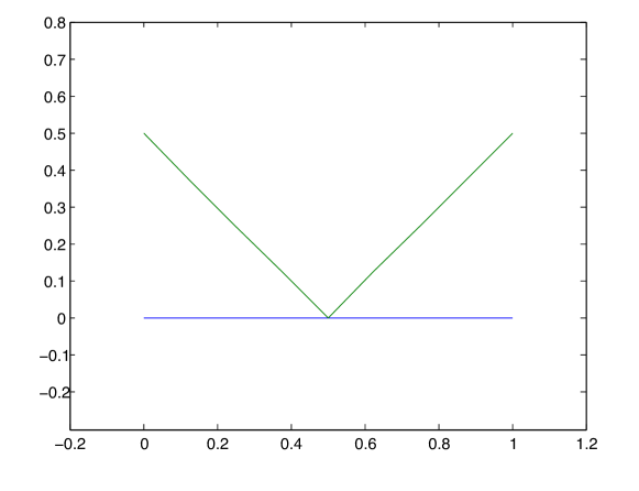
Figure 1: Shift up

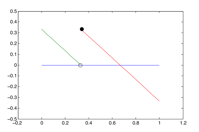
Figure 2: Shift down

Example C.4.

Let $O=(0,1)$ and

$$\omega(t)=1-t-I(t\geq 1),$$

which is illustrated in Figure 3. Since $\omega\in\Gamma_{O}$, we have the continuity of $T_{O^{c}}$ at $\omega$ by Theorem 3.2. If we take $\omega_{n}=\omega-1/n$ for all $n\in\mathbb{N}$, we have $\omega_{n}\to\omega$ in uniform topology, hence in Skorohod topology. Therefore, $T_{O^{c}}(\omega_{n})=1-1/n\to 1=T_{O^{c}}(\omega)$, which supports Theorem 3.2. However, we have

$$\Pi_{O}(\omega_{n})=0\not\to-1=\Pi_{O}(\omega).$$

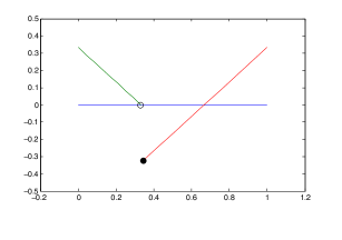
Figure 3: A small down shift makes a big change in the state at the first exit time

References

- [1] O. Alvarez and A. Tourin, Viscosity solutions of nonlinear integro-differential equations, Ann. Inst. H. Poincaré Anal. Non Linéaire, 13 (1996), pp. 293–317.
- [2] D. Applebaum, Lévy processes and stochastic calculus, vol. 93 of Cambridge Studies in Advanced Mathematics, Cambridge University Press, Cambridge, 2004.
- [3] G. Barles and J. Burdeau, The Dirichlet problem for semilinear second-order degenerate elliptic equations and applications to stochastic exit time control problems, Comm. Partial Differential Equations, 20 (1995), pp. 129–178.
- [4] G. Barles, E. Chasseigne, and C. Imbert, On the Dirichlet problem for second-order elliptic integro-differential equations, Indiana Univ. Math. J., 57 (2008), pp. 213–246.
- [5] G. Barles and C. Imbert, Second-order elliptic integro-differential equations: viscosity solutions’ theory revisited, Ann. Inst. H. Poincaré Anal. Non Linéaire, 25 (2008), pp. 567–585, https://doi.org/10.1016/j.anihpc.2007.02.007, http://dx.doi.org/10.1016/j.anihpc.2007.02.007.
- [6] G. Barles and B. Perthame, Exit time problems in optimal control and vanishing viscosity method, SIAM J. Control Optim., 26 (1988), pp. 1133–1148.
- [7] G. Barles and B. Perthame, Comparison principle for Dirichlet-type Hamilton-Jacobi equations and singular perturbations of degenerated elliptic equations, Appl. Math. Optim., 21 (1990), pp. 21–44, https://doi.org/10.1007/BF01445155, http://dx.doi.org/10.1007/BF01445155.
- [8] E. Bayraktar and M. Sîrbu, Stochastic Perron’s method and verification without smoothness using viscosity comparison: the linear case, Proc. Amer. Math. Soc., 140 (2012), pp. 3645–3654, https://doi.org/10.1090/S0002-9939-2012-11336-X, http://dx.doi.org/10.1090/S0002-9939-2012-11336-X.
- [9] E. Bayraktar and M. Sîrbu, Stochastic Perron’s method for Hamilton-Jacobi-Bellman equations, SIAM J. Control Optim., 51 (2013), pp. 4274–4294, https://doi.org/10.1137/12090352X, http://dx.doi.org/10.1137/12090352X.
- [10] E. Bayraktar and M. Sîrbu, Stochastic Perron’s method and verification without smoothness using viscosity comparison: obstacle problems and Dynkin games, Proc. Amer. Math. Soc., 142 (2014), pp. 1399–1412, https://doi.org/10.1090/S0002-9939-2014-11860-0, http://dx.doi.org/10.1090/S0002-9939-2014-11860-0.
- [11] E. Bayraktar, Q. Song, and J. Yang, On the continuity of stochastic exit time control problems, Stoch. Anal. Appl., 29 (2011), pp. 48–60, https://doi.org/10.1080/07362994.2011.532020, http://dx.doi.org/10.1080/07362994.2011.532020.
- [12] E. Bayraktar and Y. Zhang, Minimizing the probability of lifetime ruin under ambiguity aversion, SIAM J. Control Optim., 53 (2015), pp. 58–90, https://doi.org/10.1137/140955999, http://dx.doi.org/10.1137/140955999.
- [13] E. Bayraktar and Y. Zhang, Stochastic Perron’s method for the probability of lifetime ruin problem under transaction costs, SIAM J. Control Optim., 53 (2015), pp. 91–113, https://doi.org/10.1137/140967052, http://dx.doi.org/10.1137/140967052.
- [14] J. Bertoin, Lévy processes, vol. 121 of Cambridge Tracts in Mathematics, Cambridge University Press, Cambridge, 1996.
- [15] P. Billingsley, Convergence of probability measures, Wiley Series in Probability and Statistics: Probability and Statistics, John Wiley & Sons Inc., New York, second ed., 1999.
- [16] M. G. Crandall, H. Ishii, and P. L. Lions, User’s guide to viscosity solutions of second order partial differential equations, Bull. Amer. Math. Soc. (N.S.), 27 (1992), pp. 1–67.
- [17] M. V. Day, Weak convergence and fluid limits in optimal time-to-empty queueing control problems, Appl. Math. Optim., 64 (2011), pp. 339–362, https://doi.org/10.1007/s00245-011-9144-y, http://dx.doi.org/10.1007/s00245-011-9144-y.
- [18] L. C. Evans, Partial differential equations, vol. 19 of Graduate Studies in Mathematics, American Mathematical Society, Providence, RI, 1998.
- [19] W. H. Fleming and H. M. Soner, Controlled Markov processes and viscosity solutions, vol. 25 of Stochastic Modelling and Applied Probability, Springer, New York, second ed., 2006.
- [20] H. Kunita, Stochastic differential equations based on Lévy processes and stochastic flows of diffeomorphisms, in Real and stochastic analysis, Trends Math., Birkhäuser Boston, Boston, MA, 2004, pp. 305–373.
- [21] P. E. Protter, Stochastic integration and differential equations, vol. 21 of Applications of Mathematics (New York), Springer-Verlag, Berlin, second ed., 2004. Stochastic Modelling and Applied Probability.
- [22] D. B. Rokhlin, Verification by stochastic Perron’s method in stochastic exit time control problems, J. Math. Anal. Appl., 419 (2014), pp. 433–446, https://doi.org/10.1016/j.jmaa.2014.04.062, http://dx.doi.org/10.1016/j.jmaa.2014.04.062.
- [23] K. Sato, Lévy processes and infinitely divisible distributions, vol. 68 of Cambridge Studies in Advanced Mathematics, Cambridge University Press, Cambridge, 1999. Translated from the 1990 Japanese original, Revised by the author.
- [24] D. Stroock and S. R. S. Varadhan, On degenerate elliptic-parabolic operators of second order and their associated diffusions, Comm. Pure Appl. Math., 25 (1972), pp. 651–713.
- [25] E. Topp, Existence and uniqueness for integro-differential equations with dominating drift terms, Comm. Partial Differential Equations, 39 (2014), pp. 1523–1554, https://doi.org/10.1080/03605302.2014.900567, http://dx.doi.org/10.1080/03605302.2014.900567.