Abstract

We study the intersections of two sets of D-branes of different dimensionalities. This configuration is dual to a supersymmetric gauge theory with flavor hypermultiplets in the fundamental representation of the gauge group which live on the defect of the unflavored theory determined by the directions common to the two types of branes. One set of branes is dual to the color degrees of freedom, while the other set adds flavor to the system. We work in the quenched approximation, i.e., where the flavor branes are considered as probes, and focus specifically on the case in which the quarks are massive. We study the thermodynamics and the speeds of first and zero sound at zero temperature and non-vanishing chemical potential. We show that the system undergoes a quantum phase transition when the chemical potential approaches its minimal value and we obtain the corresponding non-relativistic critical exponents that characterize its critical behavior. In the case of $(2+1)$-dimensional intersections, we further study alternative quantization and the zero sound of the resulting anyonic fluid. We finally extend these results to non-zero temperature and magnetic field and compute the diffusion constant in the hydrodynamic regime. The numerical results we find match the predictions by the Einstein relation.

1 Introduction

There is hope that the gauge/gravity holographic duality could serve to characterize new types of compressible states of matter, i.e., states with non-zero charge density which vary continuously with the chemical potential. Indeed, holography provides gravitational descriptions of strongly interacting systems without long-lived quasiparticles, situations which cannot be accommodated within the standard Landau’s Fermi liquid theory. Although the field theories with known holographic dual are very different from those found so far in Nature, there are good reasons to believe that these studies could reveal generic universal features of strongly interacting quantum systems [1].

In this paper we approach this problem in a top-down model of intersecting branes of different dimensionalities. We will consider a stack of $N_{c}$ color D$p$-branes which intersect $N_{f}$ flavor D$q$-branes ($q\geq p)$ along $n$ common directions. This configuration, which we will denote by $(n\,|\,p\perp q)$, is dual to a $(p+1)$-dimensional $SU(N_{c})$ gauge theory with $N_{f}$ fundamental hypermultiplets (quarks) living on a $(n+1)$-dimensional defect [2]. In the context of holography, we will work in the large $N_{c}$ ’t Hooft limit with $N_{f}\ll N_{c}$. In this limit the quarks are quenched and the D$q$-branes can be treated as probes, whose action is the Dirac-Born-Infeld (DBI) action, in the gravitational background created by the D$p$-branes. The embedding of the flavor branes is parameterized by a function which measures the distance between the two types of branes. The field theory dual of this distance is the mass of the hypermultiplet. Moreover, in order to engineer a system with non-zero baryonic charge density, we must switch on a suitable gauge field on the worldvolume of the flavor brane [3]. We will also study the influence of a magnetic field directed along two of the spatial directions of the worldvolume.

In [4] we studied the collective excitations of generic brane intersections corresponding to massless quarks and we uncovered a certain universal structure. The purpose of this article is to extend the results of [4] to the case in which the quarks have a non-zero mass. We will study first the system at zero temperature and non-zero chemical potential. This is the so-called collisionless quantum regime, in which the dynamics is dominated by the zero sound mode. This mode is a collective excitation, first found in the holographic context in [5, 6]. These results were generalized to non-zero temperature in [7, 8] and to non-vanishing magnetic field in [9, 10] (see [11, 12, 13, 14, 15, 16, 17, 18, 19, 20, 21, 22, 23, 24, 25, 26, 27, 28] for studies on different aspects of the holographic zero sound). In [4] we developed a general formalism which included all possible intersections $(n\,|\,p\perp q)$ and, in particular, we found an index $\lambda$ (depending on $n$, $p$, and $q$) which determines the speed of zero sound for massless quarks. This is intimately related with the fact that $\lambda$ determines the scaling dimension of the charge density or to put it slightly differently, $\lambda$ acts as the polytropic index in the equation of state for the holographic matter.

In the case of massive quarks the embedding of the D$q$-brane is non-trivial and must be determined in order to extract the different physical properties. When the charge density is non-vanishing, the brane reaches the horizon of the geometry, i.e., we have a black hole embedding. This embedding depends on a function which parameterizes the shape of the flavor brane in the background geometry and, in general, must be found by numerical integration of the equations of motion of the probe. However, in the case of intersections $(n\,|\,p\perp q)$ which preserve some amount of supersymmetry at zero temperature $T$ and chemical potential $\mu$ some remarkable simplification occurs. Indeed, as shown in [29], in these intersections one can choose a system of coordinates such that the embedding function is a cyclic variable of the DBI Lagrangian when $T=0$ and $\mu\not=0$. As a consequence, the embedding function and the physical properties of the configuration, can be found analytically. In particular, one can study the zero temperature thermodynamics of these systems and find the speed of first sound. This was done in refs. [12, 13] for the D3-D$q$ intersections $(3\,|\,3\perp 7)$, $(2\,|\,3\perp 5)$, and $(1\,|\,3\perp 3)$. Moreover, by studying the quasinormal fluctuation modes of the probe, one can also compute analytically the speed of zero sound which, non-trivially, equals that of the first sound [11, 8, 30].

In this paper we generalize these results for any $(n\,|\,p\perp q)$ intersection with #ND=4, i.e., when $n=(p+q-4)/2$. These cases correspond to those brane intersections which are supersymmetric in flat space at low energies as the gravitational and Ramond-Ramond forces cancel out. Here the index $\lambda$ can only take three different values $\lambda=2,4,6$, corresponding to codimension 2 (D$p$-D$p$), codimension 1 (D$p$-D$(p+2)$), and codimension 0 (D$p$-D$(p+4)$) intersections, respectively. As in the conformal D3-background, the speeds of first and zero sounds coincide. Moreover, we find the same kind of universality as in the massless case: the speed is the same for those intersections which have the same $\lambda$ index, or codimension. However, in the massive case the speed of sound depends continuously on the chemical potential, i.e., on the charge density, and vanishes when the chemical potential reaches its minimal value, which corresponds to a vanishing charge density $d$. Actually, as argued in [30] for the D3-D7 and D3-D5 intersections, there is a quantum phase transition as $d\to 0$ which exhibits a non-relativistic scaling behavior with hyperscaling violation. At the transition point the black hole embeddings with $d\not=0$ degenerate into a Minkowski embedding with zero charge density. Here we will find the critical exponents for the general #ND=4 intersections, generalizing the results of [30].

When the number $n$ of common dimensions of the color and flavor branes is equal to two, the matter hypermultiplets live on a (2+1)-dimensional theory. In this case one can perform an alternative quantization of the quasinormal modes, which consists in imposing mixed Dirichlet-Neumann boundary conditions at the UV. As shown in [31], this alternative quantization amounts to transforming the charged excitations into particles of fractional statistics, i.e., anyons (see also [32, 33, 34, 28] for the analysis of different aspects of the holographic anyonic systems). In [4] we studied the zero sound mode as a function of the constant that measures the degree of mixing the UV boundary conditions. We found that the anyonic zero sound is generically gapped and that this gap can be fine-tuned to zero if a suitable magnetic field is switched on. This choice corresponds to the case, where the anyons experience no effective magnetic field. In this paper we generalize these results to the case in which the quarks are massive.

In this article we also study the hydrodynamic regime that is reached when the temperature is high enough. The dominant collective mode in this regime is a diffusion mode, which has a purely imaginary dispersion relation characterized by a diffusion constant $D$. When the temperature is non-zero the embedding function is no more a cyclic coordinate of the DBI action and cannot therefore be found analytically. Thus, we study this $T\not=0$ case by using numerical methods, after performing a convenient change of variables. Moreover, this numerical analysis allow us to check the analytic results found at zero temperature, by taking the $T\to 0$ limit. We also study numerically the system in the presence of a magnetic field $B$. We compare the results for the diffusion constant obtained from the fluctuation analysis at $T\not=0$ with the ones predicted by the Einstein relation, which gives $D$ in terms of the DC conductivity $\sigma$ and the charge susceptibility $\chi$. Both $\sigma$ and $\chi$ can be obtained from the embedding function. We find a very good agreement between the numerical results for $D$ and the value given by the Einstein relation.

The rest of this paper is organized as follows. In section 2 we formulate our top-down holographic model, solve the equations of motion of the probe at $T=0$ and $\mu\not=0$, and study the thermodynamics at zero temperature. In particular, in this section we find the speed of first sound and compute the charge susceptibility at $T=0$. In section 3 we write the equations of motion for the fluctuations of the probe at zero temperature. In section 4 we analyze the zero sound and find analytically the dispersion relation of this collective mode. Section 5 is devoted to the study of the scaling behavior near the quantum critical point. In section 6 we study the zero sound mode in an anyonic fluid. Section 7 contains our results at non-zero temperature and magnetic field. We summarize our results and discuss some possible future research directions in section 8.

We complement and give further details of our analysis in several appendices. Appendix A.1 contains a detailed derivation of the Lagrangian of the fluctuations at zero temperature which is used in section 3. In appendix A.2 we work out the equations of motion of the fluctuations at $T\not=0$. In appendix B we find the correlator of two transverse currents and extract the DC conductivity in the absence of magnetic field. Finally, in appendix C we provide an alternative derivation of the conductivity, valid also when $B\not=0$.

2 Massive D$p$-D$q$ systems with charge

Let us begin our analysis by introducing our setup and studying its properties at zero temperature and magnetic field. We will consider a generic D$p$-brane metric at zero temperature of the type:

$$ds_{10}^{2}\,=\,g_{tt}(r)\,dt^{2}\,+\,g_{xx}(r)\,\big{[}(dx^{1})^{2}\,+\,\cdots+(dx^{p})^{2}\big{]}\,+\,g_{rr}(r)\,d\vec{y}\cdot d\vec{y}\,\,,$$ (2.1)

where $\vec{y}\,=\,(y^{1},\ldots,y^{9-p})$ are the coordinates transverse to the D$p$-brane and the functions $g_{tt}$, $g_{xx}$, and $g_{rr}$ depend on the transverse radial direction $r=\sqrt{\vec{y}\cdot\vec{y}}$. We now embed $N_{f}$ D$q$-brane probes, with $N_{f}\ll N_{c}$, extended along the directions

$$(t,x^{1},\ldots,x^{n},y^{1},\ldots,y^{q-n})\,\,.$$ (2.2)

We will refer to this configuration as a $(n\,|\,p\perp q)$ intersection ($n$ is the number of common spatial directions of the D$p$ and D$q$). This intersection is represented by the array:

$$\begin{array}[]{cccccccccccccl}&x^{1}&\cdots&x^{n}&x^{n+1}&\cdots&x^{p}&y^{1}&\cdots&y^{q-n}&y^{q-n+1}&\cdots&y^{9-p}&\\ Dp:&\times&\cdots&\times&\times&\cdots&\times&-&\cdots&-&-&\cdots&-\\ Dq:&\times&\cdots&\times&-&\cdots&-&\times&\cdots&\times&-&\cdots&-&\end{array}$$

We shall denote by $\vec{z}$ the coordinates $\vec{y}$ transverse to the D$q$-brane:

$$\vec{z}\,=\,(z^{1},\ldots,z^{9+n-p-q})\,\,,$$ (2.3)

with $z^{m}\,=\,y^{q-n+m}$ for $m=1,\ldots,9+n-p-q$. Moreover, we define $\rho$ as the radial coordinate for the subspace spanned by $(y^{1},\ldots,y^{q-n})$:

$$\rho^{2}\,=\,(y^{1})^{2}+\cdots+(y^{q-n})^{2}\,\,.$$ (2.4)

Let us make a short comment on the global symmetries. The original D$p$-background has a rotational symmetry in the $y^{i}$ directions, this corresponds to the $SO(9-p)$ R-symmetry. When we add $N_{f}$ coincident probe D$q$-branes we introduce $U(N_{f})$ flavor symmetry. The D$p$-D$q$-intersection $(n\,|\,p\perp q)$ breaks the original R-symmetry, which can be easily read off from the isometries. We end up with the global symmetry $SO(n,1)\times U(N_{f})\times SO(p-n)_{p}\times SO(q-n)_{q}\times SO(9+n-p-q)$. The last group will be further broken when we consider massive D$q$-brane embeddings.

Since,

$$d\vec{y}^{\,\,2}\,=\,d\rho^{2}\,+\,\rho^{2}\,d\Omega^{2}_{q-n-1}\,+\,d\vec{z}^{\,\,2},$$ (2.5)

the background metric in these coordinates can be written as:

$$ds_{10}^{2}\,=\,g_{tt}(r)\,dt^{2}\,+\,g_{xx}(r)\,\Big{[}(dx^{1})^{2}\,+\,\cdots+(dx^{n})^{2}\,+\,(dx^{n+1})^{2}\,+\,\cdots+(dx^{p})^{2}\,\Big{]}$$

$$\qquad\qquad\qquad\qquad\qquad\qquad+\,g_{rr}(r)\,\Big{[}\,d\rho^{2}\,+\,\rho^{2}\,d\Omega^{2}_{q-n-1}\,+\,d\vec{z}^{\,\,2}\,\Big{]}\,\,.$$ (2.6)

Let us consider a stack of D$q$-branes with a non-trivial profile in the transverse space. We will choose our transverse coordinates in such a way that this profile can be parameterized as $\vec{z}=(z^{1}(\rho),0,\ldots,0)$. In what follows we just write $z(\rho)$ instead of $z^{1}(\rho)$ and we will denote by $r=r(\rho)$ the function:

$$r(\rho)\,=\,\sqrt{\rho^{2}+z(\rho)^{2}}\,\,.$$ (2.7)

The induced metric on the D$q$-brane worldvolume at zero temperature is:

$$ds_{q+1}^{2}=g_{tt}(\rho)\,dt^{2}+g_{xx}(\rho)\,\big{[}(dx^{1})^{2}+\cdots+(dx^{n})^{2}\,\big{]}+g_{rr}(\rho)\big{[}(1+z^{\prime\,2})\,d\rho^{2}+\rho^{2}\,d\Omega^{2}_{q-n-1}\,\big{]}\,\,,$$ (2.8)

with $z^{\prime}=dz/d\rho$. Let us compute the DBI action of the D$q$-brane in the case in which there is a worldvolume gauge field $F$ with components $\rho t$. Thus, we will take $F$ to be given by:

$$F\,=\,A_{t}^{\prime}\,d\rho\wedge dt\,\,.$$ (2.9)

where $A_{t}^{\prime}=\partial_{\rho}A_{t}$ and we have chosen a gauge for $A$ such that $A_{\rho}=0$. This means that we aim to study holographic matter at non-zero baryon charge density by introducing a chemical potential for the diagonal $U(1)\subset U(N_{f})$. The DBI action becomes:

$$S_{Dq}\,=-\,N_{f}T_{Dq}\,\int d^{q+1}\xi\,e^{-\phi}\,\sqrt{-\det(g+2\pi\alpha^{\prime}F)}\,=\,\int dt\,d^{n}x\,d\rho\,{\cal L}_{DBI}\,\,,$$ (2.10)

with the Lagrangian density ${\cal L}_{DBI}$ given by:

$${\cal L}_{DBI}\,=\,-{\cal N}\,e^{-\phi}\,\rho^{q-n-1}\,g_{xx}^{\frac{n}{2}}\,g_{rr}^{{q-n-1\over 2}}\,\sqrt{g_{rr}|g_{tt}|\,(1+z^{\prime\,2})\,-(2\pi\alpha^{\prime})^{2}\,A_{t}^{\prime 2}}\,\,,$$ (2.11)

where ${\cal N}$ is the normalization factor

$${\cal N}\,=\,N_{f}T_{Dq}\,{\rm Vol}({\mathbb{S}}^{q-n-1})\,\,,$$ (2.12)

and where the tension of the D$q$-brane and the volume of the unit sphere are

$$T_{Dq}=\frac{1}{(2\pi)^{q}\sqrt{\alpha^{\prime}}^{q+1}g_{s}}\ ,\ \ {\rm Vol}({\mathbb{S}}^{q-n-1})=\frac{2\pi^{\frac{q-n}{2}}}{\Gamma\left(\frac{q-n}{2}\right)}\ .$$ (2.13)

For a D$p$-brane background at zero temperature, the metric and the dilaton are given by:

$$-g_{tt}\,=\,g_{xx}\,=\,\Big{(}{r\over R}\Big{)}^{{7-p\over 2}}\,\,,\qquad g_{rr}\,=\,\Big{(}{R\over r}\Big{)}^{{7-p\over 2}}\,\,,\qquad e^{-2\phi}\,=\,\Big{(}{R\over r}\Big{)}^{{(7-p)(p-3)\over 2}}\,\,.$$ (2.14)

This background satisfies $g_{rr}|g_{tt}|=1$ and the Lagrangian density ${\cal L}_{DBI}$ can be written as:

$${\cal L}_{DBI}\,=\,-{\cal N}\,\rho^{q-n-1}\,\Big{(}{r\over R}\Big{)}^{{(2n-p-q+4)(7-p)\over 4}}\sqrt{1+z^{\prime\,2}\,-(2\pi\alpha^{\prime})^{2}\,A_{t}^{\prime 2}}\,\,.$$ (2.15)

In the following we will scale out the constant $R$, i.e., we will take directly $R=1$. To avoid clutter, we also redefine the gauge field by absorbing the factors of the string length $2\pi\alpha^{\prime}A_{\mu}\to A_{\mu}$. Moreover, we will restrict ourselves to the case in which the embedding function $z(\rho)$ is a cyclic variable, i.e., when ${\cal L}_{DBI}$ depends on $z^{\prime}$ and not on $z$. The only dependence on $z$ in (2.15) is the one induced by the power of $r$ multiplying the DBI square root. Therefore $z(\rho)$ is cyclic only when the following condition between $n$, $p$, and $q$ is satisfied:

$$n\,=\,{p+q-4\over 2}\,\,.$$ (2.16)

One can check that this happens only in the supersymmetric intersections with #ND=4: $(p\,|\,p\perp p+4)$, $(p-1\,|\,p\perp p+2)$, and $(p-2\,|\,p\perp p)$. In the following we will restrict ourselves to these cases. Let us define $\lambda$ as:

$$\lambda\,=\,2(q-n-1)\,=\,q-p+2\,\,.$$ (2.17)

Notice that $\lambda=6,4,2$ for the intersections D$p$-D$(p+4)$, D$p$-D$(p+2)$, and D$p$-D$p$, respectively. We can then write the Lagrangian density as:

$${\cal L}_{DBI}\,=\,-{\cal N}\,\rho^{{\lambda\over 2}}\,\sqrt{1+z^{\prime\,2}\,-\,A_{t}^{\prime 2}}\,\,.$$ (2.18)

The cyclic nature of $z$ and $A_{t}$ implies the following conservation laws:

$${1\over{\cal N}}{\partial{\cal L}_{DBI}\over\partial z^{\prime}}\,=\,-{\rho^{{\lambda\over 2}}\,z^{\prime}\over\sqrt{1+z^{\prime\,2}\,-\,A_{t}^{\prime 2}}}\,\equiv-c$$

$${1\over{\cal N}}{\partial{\cal L}_{DBI}\over\partial A_{t}^{\prime}}\,=\,{\rho^{{\lambda\over 2}}\,A_{t}^{\prime}\over\sqrt{1+z^{\prime\,2}\,-\,A_{t}^{\prime 2}}}\,\equiv d\,\,,$$ (2.19)

with $c$ and $d$ being constants of integration. These relations can be inverted as:

$$z^{\prime}\,=\,{c\over\sqrt{\rho^{\lambda}\,+\,d^{2}-c^{2}}}\,\,,\qquad\qquad\qquad A_{t}^{\prime}\,=\,{d\over\sqrt{\rho^{\lambda}\,+\,d^{2}-c^{2}}}\,\,.$$ (2.20)

When $c=d=0$, both $z(\rho)$ and $A_{t}(\rho)$ are constant and we have a Minkowski embedding. Let us suppose that $c$ does not vanish. Then, it follows from (2.20) that $A_{t}^{\prime}$ and $z^{\prime}$ are related as:

$$A_{t}^{\prime}\,=\,{d\over c}\,z^{\prime}\,\,.$$ (2.21)

When $c^{2}=d^{2}\not=0$ both $z(\rho)$ and $A_{t}(\rho)$ diverge at $\rho=0$. Therefore, we discard this configuration and we will assume in the following that $d^{2}>c^{2}$. In this case, from the expression of $z^{\prime}$ and $A_{t}^{\prime}$ written in (2.20) it is easy to conclude that the point $\rho=0$ is reached. In what follows we will assume that this condition holds. We will integrate the equation for $A_{t}(\rho)$ by imposing that $A_{t}(0)=0$. We have:

$$A_{t}(\rho)\,=\,d\,\int_{0}^{\rho}\,{d\bar{\rho}\over\sqrt{\bar{\rho}^{\lambda}+d^{2}-c^{2}}}\,\,.$$ (2.22)

This integral can be computed analytically and expressed in terms of the hypergeometric function as:

$$A_{t}(\rho)\,=\,{d\over\big{(}d^{2}-c^{2}\big{)}^{{1\over 2}-{1\over\lambda}}}\,{\rho\over\big{[}\rho^{\lambda}+d^{2}-c^{2}\big{]}^{{1\over\lambda}}}\,\,F\Big{(}\,{1\over\lambda},{1\over 2}+{1\over\lambda};1\,+\,{1\over\lambda};{\rho^{\lambda}\over\rho^{\lambda}+d^{2}-c^{2}}\,\Big{)}\,\,.$$ (2.23)

Similarly, the embedding function $z(\rho)$ can be written as:

$$z(\rho)\,=\,{c\over\big{(}d^{2}-c^{2}\big{)}^{{1\over 2}-{1\over\lambda}}}\,{\rho\over\big{[}\rho^{\lambda}+d^{2}-c^{2}\big{]}^{{1\over\lambda}}}\,\,F\Big{(}\,{1\over\lambda},{1\over 2}+{1\over\lambda};1\,+\,{1\over\lambda};{\rho^{\lambda}\over\rho^{\lambda}+d^{2}-c^{2}}\,\Big{)}\,\,.$$ (2.24)

Notice that when $d^{2}>c^{2}$ the brane reaches the Poincaré horizon of the metric at $\rho=z=0$ and we have a black hole embedding. The two constants $d$ and $c$ are related to the charge density and condensate of the dual theory, respectively.

2.1 Zero temperature thermodynamics

Let us first consider the intersections with $\lambda>2$. We also restrict to $T=0$, as at non-zero temperature not much can be said analytically. In this case the functions $A_{t}(\rho)$ and $z(\rho)$ in (2.23) and (2.24) approach a constant value in the UV region $\rho\to\infty$. According to the standard AdS/CFT dictionary, the flavor chemical potential $\mu$ is the UV value of $A_{t}$:

$$\mu\,=\,A_{t}(\rho\to\infty)\,=\,{d\over\big{(}d^{2}-c^{2}\big{)}^{{1\over 2}-{1\over\lambda}}}\,F\Big{(}\,{1\over\lambda},{1\over 2}+{1\over\lambda};1\,+\,{1\over\lambda};1\Big{)}=\,{d\over\Big{(}d^{2}-c^{2}\Big{)}^{{1\over 2}-{1\over\lambda}}}\,\gamma\ ,$$ (2.25)

where $\gamma$ is the constant

$$\gamma\,=\,{1\over\sqrt{\pi}}\,\Gamma\Big{(}{1\over 2}-{1\over\lambda}\Big{)}\,\Gamma\Big{(}1+{1\over\lambda}\Big{)}$$ (2.26)

and we used the identity $F(A,B;C;1)\,=\,{\Gamma(C)\,\Gamma(C-A-B)\over\Gamma(C-A)\,\Gamma(C-B)}$.

The mass parameter $m$ of the embedding is defined as $m=z(\rho\to\infty)$. It follows from (2.24) that:

$$m\,=\,{c\over\Big{(}d^{2}-c^{2}\Big{)}^{{1\over 2}-{1\over\lambda}}}\,\gamma\,\,.$$ (2.27)

Let us invert (2.25) and (2.27) and compute $c$ and $d$ in terms of $\mu$ and $m$. First, we notice that:

$$\mu^{2}\,-\,m^{2}\,=\,\Big{(}d^{2}-c^{2}\Big{)}^{{2\over\lambda}}\,\gamma^{2}\,\,.$$ (2.28)

Since $d^{2}\geq c^{2}$, eq. (2.28) implies that $\mu\geq m$ for the embeddings we are considering. Moreover, from (2.28) we get $d^{2}-c^{2}$ as a function of $\mu$ and $m$ and, using this result in (2.25) and (2.27), we obtain

$$c\,=\,m\,\gamma^{-{\lambda\over 2}}\,\Big{(}\mu^{2}-m^{2}\Big{)}^{{\lambda-2\over 4}}\,\,,\qquad\qquad\qquad d\,=\,\mu\,\gamma^{-{\lambda\over 2}}\,\Big{(}\mu^{2}-m^{2}\Big{)}^{{\lambda-2\over 4}}\,\,.$$ (2.29)

When $\lambda>2$, $\mu=m$ in (2.29) corresponds to $c=d=0$, i.e., to the Minkowski embeddings with vanishing density discussed above. Actually, as illustrated in Fig. 1, the topology of the embeddings changes when $m\to\mu$, where a quantum phase transition takes place. The order parameter of this transition is the charge density (see [29] for further details).

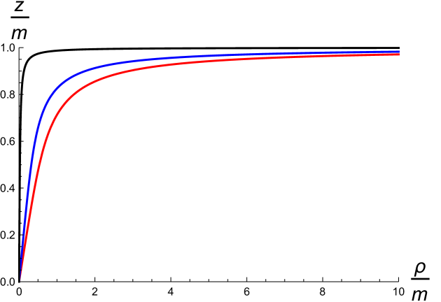
Figure 1: In this figure we plot the different embeddings for $\lambda=4$ and $m/\mu=0.1,\,0.8,\,0.999$ (bottom-up). The Minkowski embeddings at zero density and $m/\mu=1$ would correspond to the constant horizontal line $z/m=1$.

Let us now evaluate the on-shell action of the probe. Using

$$\sqrt{1+z^{\prime\,2}\,-\,A_{t}^{\prime 2}}\Big{|}_{on-shell}\,=\,{\rho^{{\lambda\over 2}}\over\sqrt{\rho^{\lambda}\,+\,d^{2}-c^{2}}}\,\,,$$ (2.30)

we find

$$S_{on-shell}\,=\,-{\cal N}\,\,\int_{0}^{\infty}\,{\rho^{\lambda}\over\sqrt{\rho^{\lambda}\,+\,d^{2}-c^{2}}}\,d\rho\,\,,$$ (2.31)

which is divergent and must be regulated. We will do it by subtracting the same integral with the integrand evaluated at the UV ($\rho\to\infty$). We arrive at

$$S_{on-shell}^{reg}\,=\,-{\cal N}\,\,\int_{0}^{\infty}\,\rho^{{\lambda\over 2}}\,\Bigg{[}\,{\rho^{{\lambda\over 2}}\over\sqrt{\rho^{\lambda}\,+\,d^{2}-c^{2}}}\,-\,1\Bigg{]}\,d\rho\,=\,{2\,{\cal N}\over\lambda+2}\,\Big{(}d^{2}-c^{2}\Big{)}^{{1\over\lambda}+{1\over 2}}\,\gamma\,\,.$$ (2.32)

The zero-temperature grand canonical potential $\Omega$ is given by minus the regulated on-shell action:

$$\Omega\,=\,-S_{on-shell}^{reg}\,=\,-{2\,{\cal N}\over\lambda+2}\,\Big{(}d^{2}-c^{2}\Big{)}^{{1\over\lambda}+{1\over 2}}\,\gamma\,\,.$$ (2.33)

In terms of $m$ and $\mu$ the grand canonical potential can be written as:

$$\Omega\,=\,-{2\,{\cal N}\over\lambda+2}\,\gamma^{-{\lambda\over 2}}\,\Big{(}\mu^{2}-m^{2}\Big{)}^{{\lambda+2\over 4}}\,\,,$$ (2.34)

where we have used (2.28). Moreover, the charge density is:

$$\rho_{ch}\,=\,-{\partial\Omega\over\partial\mu}\,=\,\mu{\cal N}\gamma^{-{\lambda\over 2}}\,\Big{(}\mu^{2}-m^{2}\Big{)}^{{\lambda-2\over 4}}\,=\,{\cal N}\,d\,\,,$$ (2.35)

which confirms our identification of the constant $d$. It is worth noting that the formulas that we will write down do not have the factor of the (infinite) volume of the gauge theory directions $V_{\mathbb{R}^{n}}$, rather all thermodynamic quantities are densities per unit volume. Next, we compute the energy density as:

$$\epsilon\,=\,\Omega+\mu\,\rho_{ch}\,=\,{{\cal N}\over(\lambda+2)}\,\gamma^{-{\lambda\over 2}}\,\Big{(}\mu^{2}-m^{2}\Big{)}^{{\lambda-2\over 4}}\,(\lambda\mu^{2}+2m^{2})\,\,.$$ (2.36)

To calculate the speed of first sound $u_{s}$ we make use of the equation

$$u_{s}^{2}\,=\,{\partial P\over\partial\epsilon}\,=\,{\partial P\over\partial\mu}\Big{(}{\partial\epsilon\over\partial\mu}\Big{)}^{-1}\,\,,$$ (2.37)

where $P$ is the pressure. Let us first compute the derivative appearing in the numerator. Since $P=-\Omega$, we get from (2.34):

$${\partial P\over\partial\mu}\,=\,\mu\,{\cal N}\,\gamma^{-{\lambda\over 2}}\,\Big{(}\mu^{2}-m^{2}\Big{)}^{{\lambda-2\over 4}}\,\,.$$ (2.38)

Moreover, from (2.36) we have:

$${\partial\epsilon\over\partial\mu}\,=\,\mu\,{\cal N}\,\gamma^{-{\lambda\over 2}}\,\Big{(}\mu^{2}-m^{2}\Big{)}^{{\lambda-6\over 4}}\,\Big{(}{\lambda\over 2}\,\mu^{2}\,-\,m^{2}\Big{)}\,\,.$$ (2.39)

These yield

$$u_{s}^{2}\,=\,2\,{\mu^{2}-m^{2}\over\lambda\,\mu^{2}\,-\,2\,m^{2}}\,\,,$$ (2.40)

which is the result we were looking for. As a check notice that (2.40) gives $u_{s}^{2}=2/\lambda$ for $m=0$, which is the universal result found in [4]. Moreover, the speed of sound (2.40) depends on the integers $(n,p,q)$ through the combination $\lambda$, i.e., $u_{s}$ is the same for conformal and non-conformal brane backgrounds with the same index $\lambda$. In particular, for the D3-D7 and D3-D5 supersymmetric intersections we have:

$$u_{s}^{2}\,=\,{\mu^{2}-m^{2}\over 3\,\mu^{2}\,-\,m^{2}}\,\,,\qquad\qquad\qquad{\rm for\,\,D3-D7}\,\,,$$

$$u_{s}^{2}\,=\,{\mu^{2}-m^{2}\over 2\,\mu^{2}\,-\,m^{2}}\,\,,\qquad\qquad\qquad{\rm for\,\,D3-D5}\,\,.$$ (2.41)

These results agree with the calculation in [12, 13]. Notice that the speed of sound vanishes in the zero density limit with $\mu=m$, which is a clear sign of a quantum phase transition.

Let us now consider the case $\lambda=2$, which corresponds to the $(p-2|p\perp p)$ intersections. In these systems $A_{t}(\rho)$ and $z(\rho)$ grow logarithmically when $\rho\to\infty$ and the AdS/CFT dictionary must be adapted accordingly. Indeed, in this case the chemical potential and the mass are obtained from the subleading terms of $A_{t}$ and $z$ in the UV . Moreover, the on-shell action has additional logarithmic divergences, which must be eliminated with new counterterms [35, 36]. As the result of this analysis one gets that the grand canonical potential for black hole embeddings takes the form $\Omega=-a\,(\mu^{2}-m^{2})$, where $a$ is a positive constant [37]. Repeating the calculation of $u_{s}$ performed above, it is straightforward to verify that $u_{s}^{2}=1$ in this $\lambda=2$ case. Notice that this value is exactly the one obtained by taking $\lambda=2$ in (2.40).

3 Fluctuations

We now allow fluctuations of both the gauge field along the Minkowski directions of the intersection and of the scalar function in the form:

$$A_{\nu}\,=\,A_{\nu}^{(0)}\,+\,a_{\nu}(\rho,x^{\mu})\,\,,\qquad\qquad z\,=\,z_{0}(\rho)\,+\,\xi(\rho,x^{\mu})\,\,,$$ (3.1)

where $A^{(0)}=A_{\nu}^{(0)}\,dx^{\nu}=A_{t}\,dt$ is the one-form for the unperturbed gauge field (2.23) and $z_{0}$ is the embedding function written in (2.24). The total gauge field strength is:

$$F\,=\,F^{(0)}\,+\,f\,\,,$$ (3.2)

with $F^{(0)}=dA^{(0)}$ and $f=da$. The dynamics of the fluctuations is determined by the Lagrangian density ${\cal L}$ that results after expanding the DBI action to second order in the perturbations $a_{\mu}$ and $\xi$. The detailed calculation of ${\cal L}$ is performed in appendix A.1. The Lagrangian can be neatly written in terms of open string metric ${\cal G}^{ab}$, which is symmetric and has the following non-vanishing components:

$${\cal G}^{tt} = -{\rho^{\lambda}+d^{2}\over(\rho^{2}+z_{0}^{2})^{{7-p\over 4}}\,\rho^{\lambda}}$$

$${\cal G}^{\rho\rho} = (\rho^{2}+z_{0}^{2})^{{7-p\over 4}}\,\,{\rho^{\lambda}+d^{2}-c^{2}\over\rho^{\lambda}}$$

$${\cal G}^{x^{i}\,x^{j}} = {\delta^{ij}\over(\rho^{2}+z_{0}^{2})^{{7-p\over 4}}}\,\,.$$ (3.3)

The Lagrangian density for the fluctuations can be written as:

$${\cal L}\,=\,-{\cal N}\,{\rho^{\lambda}\over\sqrt{\rho^{\lambda}+d^{2}-c^{2}}}\Bigg{[}{1\over 4}\,{\cal G}^{ac}\,{\cal G}^{bd}\,f_{cd}\,f_{ab}\,+\,{1\over 2r_{0}^{{7-p\over 2}}}\,\Big{(}1-{c^{2}\over\rho^{\lambda}}\Big{)}\,{\cal G}^{ab}\,\partial_{a}\xi\,\partial_{b}\xi\,\qquad\qquad$$

$$\qquad\qquad\qquad\qquad\qquad\qquad\qquad-{c^{2}\,d^{2}\over 2\,r_{0}^{7-p}\rho^{2\lambda}}\,(\partial_{t}\xi)^{2}\,-\,{cd\over r_{0}^{{7-p\over 2}}\,\rho^{\lambda}}\,{\cal G}^{ab}\,\partial_{a}\xi\,f_{tb}\,\,\Bigg{]}\,\,,\qquad$$ (3.4)

where we have defined $r_{0}=r_{0}(\rho)$ as:

$$r_{0}(\rho)\,=\,\sqrt{\rho^{2}+z_{0}(\rho)^{2}}\,\,.$$ (3.5)

In (3.4) the tensor indices $a,b,c,d$ run over the directions $(\rho,x^{\mu})$.

Let us now explicitly write down the equations of motion derived from the Lagrangian (3.4). We will choose the gauge in which $a_{\rho}=0$. Moreover, we will consider fluctuation fields $a_{\nu}$ which depend on $\rho$, $t$, and $x^{1}$. Then, it is possible to restrict to the case in which $a_{\nu}\not=0$ only when $\nu=t,x^{1}\equiv x$, and $x^{2}\equiv y$. The equation of motion for $a_{\rho}$ when $a_{\rho}=0$ leads to the following transversality condition:

$$\Big{(}1+{d^{2}\over\rho^{\lambda}}\Big{)}\,\partial_{t}\,a_{t}^{\prime}\,-\,{c\,d\over\rho^{\lambda}}\,\partial_{t}\,\xi^{\prime}\,-\,\partial_{x}\,a_{x}^{\prime}\,=\,0\,\,.$$ (3.6)

Let us Fourier transform the gauge and scalar fields to momentum space as:

$$a_{\nu}(\rho,t,x) = \int{d\omega\,dk\over(2\pi)^{2}}\,a_{\nu}(\rho,\omega,k)\,e^{-i\omega\,t\,+\,ikx}$$

$$\xi(\rho,t,x) = \int{d\omega\,dk\over(2\pi)^{2}}\,\xi(\rho,\omega,k)\,e^{-i\omega\,t\,+\,ikx}\,\,.$$ (3.7)

In momentum space the transversality condition (3.6) takes the form:

$$\Big{(}1+{d^{2}\over\rho^{\lambda}}\Big{)}\,\omega\,a_{t}^{\prime}\,-\,{c\,d\over\rho^{\lambda}}\,\omega\,\xi^{\prime}\,+\,k\,a_{x}^{\prime}\,=\,0\,\,.$$ (3.8)

Let us now define the electric field $E$ as the gauge-invariant combination:

$$E\,=\,k\,a_{t}\,+\,\omega\,a_{x}\,\,.$$ (3.9)

Using (3.8) we can obtain $a_{t}^{\prime}$ and $a_{x}^{\prime}$ in terms of $E^{\prime}$ and $\xi^{\prime}$ as follows:

$$a_{t}^{\prime}\,=\,{k\,\rho^{\lambda}\,E^{\prime}\,-\,c\,d\,\omega^{2}\,\xi^{\prime}\over\rho^{\lambda}\,k^{2}\,-\,(\rho^{\lambda}+d^{2})\,\omega^{2}}\,\,,\qquad\qquad a_{x}^{\prime}\,=\,{\omega\over\rho^{\lambda}\,k^{2}\,-\,(\rho^{\lambda}+d^{2})\,\omega^{2}}\,\big{[}\,c\,d\,k\xi^{\prime}\,-\,(\rho^{\lambda}+d^{2})\,E^{\prime}\big{]}\,\,.$$ (3.10)

The equation of motion for $a_{t}$ derived from (3.4) is:

$$\partial_{\rho}\Bigg{[}\,{\sqrt{\rho^{\lambda}+d^{2}-c^{2}}\over\rho^{\lambda}}\Big{[}(\rho^{\lambda}+d^{2})a_{t}^{\prime}\,-\,c\,d\,\xi^{\prime}\Big{]}\Bigg{]}$$

$$\qquad\qquad-{1\over r_{0}^{7-p}\sqrt{\rho^{\lambda}+d^{2}-c^{2}}}\Big{[}(\rho^{\lambda}+d^{2})\partial_{x}\,(\partial_{t}a_{x}-\partial_{x}a_{t})\,+\,c\,d\,\partial^{2}_{x}\xi\,\Big{]}\,=\,0\,\,.\qquad\qquad$$ (3.11)

The equation for $a_{x}$ is:

$$\partial_{\rho}\Big{(}\sqrt{\rho^{\lambda}+d^{2}-c^{2}}a_{x}^{\prime}\Big{)}-{1\over r_{0}^{7-p}\sqrt{\rho^{\lambda}+d^{2}-c^{2}}}\big{[}(\rho^{\lambda}+d^{2})\partial_{t}(\partial_{t}a_{x}-\partial_{x}a_{t})+cd\partial_{t}\partial_{x}\xi\big{]}=0\ .$$ (3.12)

By using (3.10), eqs. (3.11) and (3.12) reduce (in momentum space) to the following equation in terms of the electric field $E$:

$$\partial_{\rho}\Big{[}{\sqrt{\rho^{\lambda}+d^{2}-c^{2}}\over(\omega^{2}-k^{2})\rho^{\lambda}+\omega^{2}d^{2}}\,\big{[}(\rho^{\lambda}+d^{2})E^{\prime}\,-\,cd\,k\,\xi^{\prime}\big{]}\Big{]}+{(\rho^{\lambda}+d^{2})E-cd\,k\,\xi\over r_{0}^{7-p}\sqrt{\rho^{\lambda}+d^{2}-c^{2}}}=0\,\,.$$ (3.13)

The equation for $a_{y}$ in momentum space is:

$$\partial_{\rho}\,\Big{(}\sqrt{\rho^{\lambda}+d^{2}-c^{2}}\,a_{y}^{\prime}\Big{)}+{(\rho^{\lambda}+d^{2})\,\omega^{2}-\rho^{\lambda}\,k^{2}\over r_{0}^{7-p}\sqrt{\rho^{\lambda}+d^{2}-c^{2}}}\,a_{y}\,=\,0\,\,.$$ (3.14)

Finally, the equation for the scalar $\xi$ in momentum space can be written as:

$$\partial_{\rho}\Bigg{[}\,{\sqrt{\rho^{\lambda}+d^{2}-c^{2}}\over\rho^{\lambda}}\Big{[}(\rho^{\lambda}-c^{2})\,\xi^{\prime}+cd\,a_{t}^{\prime}\Big{]}\Bigg{]}$$

$$\qquad\qquad\qquad\qquad\qquad\qquad+{[(c^{2}-\rho^{\lambda})k^{2}\,+\,(\rho^{\lambda}+d^{2}-c^{2})\omega^{2}]\xi-cd\,k\,E\over r_{0}^{7-p}\sqrt{\rho^{\lambda}+d^{2}-c^{2}}}\,=\,0\,\,.\qquad\qquad$$ (3.15)

By using (3.10) we can rewrite this equation in terms of the electric field $E$:

$$\partial_{\rho}\Bigg{[}\,{\sqrt{\rho^{\lambda}+d^{2}-c^{2}}\over(\omega^{2}-k^{2})\rho^{\lambda}+\omega^{2}\,d^{2}}\Big{[}[(c^{2}-\rho^{\lambda})k^{2}\,+\,(\rho^{\lambda}+d^{2}-c^{2})\omega^{2}]\xi^{\prime}-cd\,k\,E^{\prime}\Big{]}\Bigg{]}$$

$$\qquad\qquad\qquad\qquad\qquad\qquad+{[(c^{2}-\rho^{\lambda})k^{2}\,+\,(\rho^{\lambda}+d^{2}-c^{2})\omega^{2}]\xi-cd\,k\,E\over r_{0}^{7-p}\sqrt{\rho^{\lambda}+d^{2}-c^{2}}}\,=\,0\,\,.\qquad\qquad$$ (3.16)

In the next section we study these equations of motion in the regime in which the frequency $\omega$ and the momentum $k$ are small and of the same order. We will find a sound mode, the zero sound, and we will be able to determine analytically its dispersion relation following the matching technique introduced in [5].

4 Zero sound

We now study the zero sound of the massive embeddings by matching the near-horizon and low frequency behavior of the fluctuations. The technique we employ consists in performing these two limits in different order [5].

4.1 Near-horizon analysis

Let us first consider the equations of motion (3.13) and (3.16) near the Poincaré horizon $\rho\approx 0$. To perform this analysis we define the functions $\chi_{1}$ and $\chi_{2}$ as:

$$\chi_{1} = (\rho^{\lambda}+d^{2})E-cd\,k\,\xi$$

$$\chi_{2} = [(c^{2}-\rho^{\lambda})k^{2}\,+\,(\rho^{\lambda}+d^{2}-c^{2})\omega^{2}]\xi-cd\,k\,E\,\,.$$ (4.1)

For small $\rho$ we just neglect the terms containing $\rho^{\lambda}$ in the $\chi_{i}$’s. Then, these functions take the form:

$$\chi_{1}\,\approx\,d^{2}\,E-cd\,k\,\xi\,\,,\qquad\qquad\chi_{2}\,\approx\,[c^{2}\,k^{2}\,+\,(d^{2}-c^{2})\omega^{2}]\xi-cd\,k\,E\,\,,$$ (4.2)

and, therefore, are related to $E$ and $\xi$ by linear combinations with constant coefficients. In order to write the near-horizon equations for $\chi_{1}$ and $\chi_{2}$, let us study the behavior of the embedding function $z_{0}(\rho)$ for small $\rho$. From (2.24) we easily obtain:

$$z_{0}\,\approx{c\over\sqrt{d^{2}-c^{2}}}\,\rho\,\,.$$ (4.3)

It follows that $r_{0}(\rho)$ behaves near $\rho\approx 0$ as:

$$r_{0}\,\approx{d\over\sqrt{d^{2}-c^{2}}}\,\rho\,\,.$$ (4.4)

Using these results it is straightforward to demonstrate that, for small $\rho$, the $\chi_{i}$’s satisfy the equation:

$$\chi_{i}^{\prime\prime}\,+\,{\Lambda^{2}\over\rho^{7-p}}\,\chi_{i}\,=\,0\,\,,$$ (4.5)

where $\Lambda$ is the following rescaled frequency:

$$\Lambda^{2}=\Big{(}{d^{2}-c^{2}\over d^{2}}\Big{)}^{{5-p\over 2}}\,\omega^{2}\,\,.$$ (4.6)

Eq. (4.5) is the same equation as in the massless case (with $\omega\to\Lambda$). When $p<5$, the solution of this equation with incoming boundary condition at the horizon is given by the following Hankel function:

$$\chi_{i}(\rho)\,=\,\rho^{{1\over 2}}\,H_{{1\over 5-p}}^{(1)}\,\Big{(}{2\,\Lambda\over 5-p}\,\rho^{{p-5\over 2}}\Big{)}\,\,,\qquad\qquad(p<5)\,\,.$$ (4.7)

For $d\not=c$ the equations in (4.2) can be inverted and one can obtain $E$ and $\xi$ as linear combinations (with constant coefficients) of $\chi_{1}$ and $\chi_{2}$. Thus, $E$ and $\xi$ behave as in (4.7). Moreover, when $p<4$ and $\omega$ is small, we have:

$$E(\rho)\,=\,A\,\rho+A\,c_{p}\,\Lambda^{{2\over 5-p}}\,+\,\cdots\,\,,\qquad\qquad\xi(\rho)\,=\,B\,\rho+B\,c_{p}\,\Lambda^{{2\over 5-p}}\,+\,\cdots\,\,,\qquad\qquad(p<4)\,\,,$$ (4.8)

where $A$ and $B$ are constants and the coefficient $c_{p}$ is:

$$c_{p}\,=\,\pi\,{(5-p)^{{p-3\over 5-p}}\over\,\Big{[}\Gamma\Big{(}{1\over 5-p}\Big{)}\Big{]}^{2}}\,\Big{[}i\,-\,\cot\Big{(}{\pi\over 5-p}\Big{)}\Big{]}\,\,,\qquad\qquad(p<4)\,\,.$$ (4.9)

4.2 Low frequency analysis

Let us now start by taking the low frequency limit of the fluctuation equations (3.13) and (3.16). One can show that in this limit one can neglect the terms without derivatives. Then, the fluctuation equations reduce to:

$$\partial_{\rho}\Big{[}{\sqrt{\rho^{\lambda}+d^{2}-c^{2}}\over(\omega^{2}-k^{2})\rho^{\lambda}+\omega^{2}d^{2}}\,\big{[}(\rho^{\lambda}+d^{2})E^{\prime}\,-\,cd\,k\,\xi^{\prime}\big{]}\Big{]} = 0$$

$$\partial_{\rho}\Bigg{[}\,{\sqrt{\rho^{\lambda}+d^{2}-c^{2}}\over(\omega^{2}-k^{2})\rho^{\lambda}+\omega^{2}\,d^{2}}\Big{[}[(c^{2}-\rho^{\lambda})k^{2}\,+\,(\rho^{\lambda}+d^{2}-c^{2})\omega^{2}]\xi^{\prime}-cd\,k\,E^{\prime}\Big{]}\Bigg{]} = 0\,\,.\qquad\qquad$$ (4.10)

These equations can be immediately integrated once to give:

$$(\rho^{\lambda}+d^{2})E^{\prime}\,-\,cd\,k\,\xi^{\prime} = C_{1}\,{(\omega^{2}-k^{2})\rho^{\lambda}+\omega^{2}d^{2}\over\sqrt{\rho^{\lambda}+d^{2}-c^{2}}}$$

$$c\,d\,k\,E^{\prime}-[(c^{2}-\rho^{\lambda})k^{2}\,+\,(\rho^{\lambda}+d^{2}-c^{2})\omega^{2}]\xi^{\prime} = C_{2}\,{(\omega^{2}-k^{2})\rho^{\lambda}+\omega^{2}d^{2}\over\sqrt{\rho^{\lambda}+d^{2}-c^{2}}}\,\,,$$ (4.11)

where $C_{1}$ and $C_{2}$ are integration constants. Solving for $E^{\prime}$ and $\xi^{\prime}$, we get:

$$E^{\prime} = {[(\omega^{2}-k^{2})\,\rho^{\lambda}\,+\,(k^{2}-\omega^{2})\,c^{2}\,+\,\omega^{2}\,d^{2}]C_{1}\,-\,cd\,k\,C_{2}\over(\rho^{\lambda}+d^{2}-c^{2})^{{3\over 2}}}$$

$$\xi^{\prime} = {cd\,k\,C_{1}\,-\,(\rho^{\lambda}+d^{2})\,C_{2}\over(\rho^{\lambda}+d^{2}-c^{2})^{{3\over 2}}}\,\,.$$ (4.12)

In order to perform a further integration, let us define the following functions:

$${\cal J}_{1}(\rho)\,\equiv\,\int_{\rho}^{\infty}\,{\bar{\rho}^{\lambda}\over(\bar{\rho}^{\lambda}+d^{2}-c^{2})^{{3\over 2}}}\,d\bar{\rho}\,\,,\qquad\qquad{\cal J}_{2}(\rho)\,\equiv\,\int_{\rho}^{\infty}\,{d\bar{\rho}\over(\bar{\rho}^{\lambda}+d^{2}-c^{2})^{{3\over 2}}}\,\,.$$ (4.13)

For $\lambda>2$ these integrals are convergent and can be computed analytically:

$${\cal J}_{1}(\rho)\,=\,{2\over\lambda-2}\,\rho^{1-{\lambda\over 2}}\,F\Big{(}\,{3\over 2},{1\over 2}-{1\over\lambda};{3\over 2}\,-\,{1\over\lambda};-{d^{2}-c^{2}\over\rho^{\lambda}}\,\Big{)}$$

$${\cal J}_{2}(\rho)\,=\,{2\over 3\lambda-2}\,\rho^{1-{3\lambda\over 2}}\,F\Big{(}\,{3\over 2},{3\over 2}-{1\over\lambda};{5\over 2}\,-\,{1\over\lambda};-{d^{2}-c^{2}\over\rho^{\lambda}}\,\Big{)}\,\,.$$ (4.14)

Moreover, by construction ${\cal J}_{1}(\rho\to\infty)={\cal J}_{2}(\rho\to\infty)=0$. It follows that:

$$E(\rho) = E^{(0)}\,-\,(\omega^{2}-k^{2})\,C_{1}\,{\cal J}_{1}(\rho)\,-\,\Big{[}[(k^{2}-\omega^{2})\,c^{2}+\omega^{2}\,d^{2}\,]C_{1}-cd\,k\,C_{2}\Big{]}\,{\cal J}_{2}(\rho)$$

$$\xi(\rho) = \xi^{(0)}\,+\,C_{2}\,{\cal J}_{1}(\rho)\,+\,d\big{[}d\,C_{2}-c\,k\,C_{1}\big{]}\,{\cal J}_{2}(\rho)\,\,,$$ (4.15)

where $E^{(0)}$ and $\xi^{(0)}$ are the values of $E$ and $\xi$ at the boundary $\rho\to\infty$. Let us now expand $E(\rho)$ and $\xi(\rho)$ near $\rho\approx 0$. With this purpose it is better to deal directly with the integrals defining ${\cal J}_{1}$ and ${\cal J}_{2}$. One can easily prove that:

$${\cal J}_{1}(\rho) = {2\over\lambda}\,\gamma\,(d^{2}-c^{2})^{{1\over\lambda}-{1\over 2}}\,+\,{\mathcal{O}}(\rho^{2})$$

$${\cal J}_{2}(\rho) = {\lambda-2\over\lambda}\,\gamma\,(d^{2}-c^{2})^{{1\over\lambda}-{3\over 2}}\,-\,{\rho\over(d^{2}-c^{2})^{{3\over 2}}}\,+\,{\mathcal{O}}(\rho^{2})\,\,,$$ (4.16)

where $\gamma$ is the constant defined in (2.26). Using these expansions we can represent $E(\rho)$ near the horizon as:

$$E(\rho)\,=\,E^{(0)}\,+\,b_{1}\,C_{1}\,+b_{2}\,C_{2}\,+\,(a_{1}\,C_{1}\,+\,a_{2}\,C_{2})\,\rho\,+\,\cdots\,\,,$$ (4.17)

where the coefficients $b_{i}$ and $a_{i}$ are given by:

$$b_{1} = -{\gamma\over\lambda}\,(d^{2}-c^{2})^{{1\over\lambda}-{3\over 2}}\,\Big{[}\,(\lambda c^{2}\,-\,2\,d^{2})\,k^{2}\,+\,\lambda\,(d^{2}-c^{2})\,\omega^{2}\,\Big{]}$$

$$b_{2} = {\lambda-2\over\lambda}\,\gamma\,(d^{2}-c^{2})^{{1\over\lambda}-{3\over 2}}\,c\,d\,k$$

$$a_{1} = {(d^{2}-c^{2})\omega^{2}\,+\,c^{2}\,k^{2}\over(d^{2}-c^{2})^{{3\over 2}}}$$

$$a_{2} = -{c\,d\,k\over(d^{2}-c^{2})^{{3\over 2}}}\,\,.$$ (4.18)

Similarly, $\xi(\rho)$ can be expanded as:

$$\xi(\rho)\,=\,\xi^{(0)}\,+\,\tilde{b}_{1}\,C_{1}\,+\tilde{b}_{2}\,C_{2}\,+\,(\tilde{a}_{1}\,C_{1}\,+\,\tilde{a}_{2}\,C_{2})\,\rho\,+\,\cdots\,\,,$$ (4.19)

where the different coefficients are:

$$\tilde{b}_{1} = -{\lambda-2\over\lambda}\,\gamma\,(d^{2}-c^{2})^{{1\over\lambda}-{3\over 2}}\,c\,d\,k\,=\,-b_{2}$$

$$\tilde{b}_{2} = {\gamma\over\lambda}\,(d^{2}-c^{2})^{{1\over\lambda}-{3\over 2}}\,(\lambda\,d^{2}\,-\,2\,c^{2})$$

$$\tilde{a}_{1} = {c\,d\,k\over(d^{2}-c^{2})^{{3\over 2}}}\,=\,-a_{2}$$

$$\tilde{a}_{2} = -{d^{2}\over(d^{2}-c^{2})^{{3\over 2}}}\,\,.$$ (4.20)

4.3 Matching

We now match (4.17) and (4.19) with (4.8). By identifying the terms linear in $\rho$, we can write the constants $A$ and $B$ of (4.8) in terms of the coefficients of (4.18) and (4.20):

$$A = a_{1}\,C_{1}\,+\,a_{2}\,C_{2}\,=\,{\big{[}(d^{2}-c^{2})\,\omega^{2}\,+\,c^{2}\,k^{2}\big{]}\,C_{1}\,-\,c\,d\,k\,C_{2}\over(d^{2}-c^{2})^{{3\over 2}}}$$

$$B = \tilde{a}_{1}\,C_{1}\,+\,\tilde{a}_{2}\,C_{2}\,=\,{c\,d\,k\,C_{1}\,-\,d^{2}\,C_{2}\over(d^{2}-c^{2})^{{3\over 2}}}\,\,.$$ (4.21)

By eliminating $A$ and $B$ and comparing the constant terms in (4.8), (4.17), and (4.19) we get the boundary values of $E$ and $\xi$ as functions of $C_{1}$ and $C_{2}$:

$$\begin{pmatrix}E^{(0)}\\ \\ \xi^{(0)}\end{pmatrix}\,=\,\begin{pmatrix}\Lambda^{{2\over 5-p}}\,c_{p}\,a_{1}\,-\,b_{1}&&&\Lambda^{{2\over 5-p}}\,c_{p}\,a_{2}\,-\,b_{2}\\ {}&{}\\ \Lambda^{{2\over 5-p}}\,c_{p}\,\tilde{a}_{1}\,-\,\tilde{b}_{1}&&&\Lambda^{{2\over 5-p}}\,c_{p}\,\tilde{a}_{2}\,-\,\tilde{b}_{2}\end{pmatrix}\,\begin{pmatrix}C_{1}\\ \\ C_{2}\end{pmatrix}\,\,.$$ (4.22)

We now require the vanishing of the sources $E^{(0)}$ and $\xi^{(0)}$, which only happens non-trivially if the determinant of the matrix written in (4.22) is zero. This leads to the following relation:

$$(\,a_{1}\,\tilde{a}_{2}+a_{2}^{2}\,)\,\Lambda^{{4\over 5-p}}\,c_{p}^{2}\,-\,(a_{1}\,\tilde{b}_{2}\,+\,\tilde{a}_{2}\,b_{1}\,+\,2\,a_{2}\,b_{2}\,)\,\Lambda^{{2\over 5-p}}\,c_{p}\,+\,b_{1}\,\tilde{b}_{2}\,+\,b_{2}^{2}\,=\,0\,\,.$$ (4.23)

From (4.23) we can find the dispersion relation of the zero sound modes. Indeed, let us assume that $\omega\sim k\sim{\mathcal{O}}(\epsilon)$. Then, $\Lambda\sim{\mathcal{O}}(\epsilon)$ and the orders of the different coefficients in (4.23) are:

$$b_{1}\sim a_{1}\sim{\mathcal{O}}(\epsilon^{2})\,\,,\qquad b_{2}\sim a_{2}\sim{\mathcal{O}}(\epsilon)\,\,,\qquad\tilde{b}_{1}\sim\tilde{a}_{1}\sim{\mathcal{O}}(\epsilon)\,\,,\qquad\tilde{b}_{2}\sim\tilde{a}_{2}\sim{\mathcal{O}}(\epsilon^{0})\,\,.$$ (4.24)

At leading order the only contribution comes from the last two terms in (4.23), which therefore reduces to:

$$b_{1}\,\tilde{b}_{2}\,+\,b_{2}^{2}\,=\,0\,\,.$$ (4.25)

By using the values of the constants $b_{1}$, $b_{2}$, and $\tilde{b}_{2}$ from (4.18) and (4.20) it is straightforward to verify that (4.25) leads to the following dispersion relation:

$$\omega^{2}\,=\,\omega^{2}_{0}\,=\,{2(d^{2}-c^{2})\over\lambda\,d^{2}-2\,c^{2}}\,k^{2}\,\,.$$ (4.26)

Let us write this result in terms of the reduced mass parameter ${\bf m}$, defined as:

$${\bf m}\,=\,{m\over\mu}\,\,.$$ (4.27)

One easily checks that:

$${c\over d}\,=\,{\bf m}\,\,.$$ (4.28)

and the leading dispersion relation can be written as:

$$\omega^{2}_{0}\,=\,c_{s}^{2}\,k^{2}\,\,,$$ (4.29)

where $c_{s}$ is the speed of zero sound, given by

$$c_{s}^{2}\,=\,2\,\,{1-{\bf m}^{2}\over\lambda\,-2\,{\bf m}^{2}}\,\,.$$ (4.30)

Notice that, non-trivially, $c_{s}$ is equal to the speed of first sound written in (2.40).

Let us now compute the next order in the dispersion relation. We write:

$$\omega\,=\,\omega_{0}\,+\,\delta\omega\,\,.$$ (4.31)

At first-order in $\delta\omega$, we get:

$$\delta\omega\,=\,-\,2^{{p-3\over 2(5-p)}}\,c_{p}\,{\lambda\,d\over\gamma}\,{(d^{2}-c^{2})^{{6-p\over 5-p}-{1\over\lambda}}\over(\lambda\,d^{2}-2c^{2})^{{7-p\over 2(5-p)}+1}}\,k^{{7-p\over 5-p}}\,\,.$$ (4.32)

In terms of ${\bf m}$ this expression becomes:

$$\delta\omega\,=\,-\,2^{{p-3\over 2(5-p)}}\,c_{p}\,{\lambda\,\over\mu}\,{(1-{\bf m}^{2})^{{6-p\over 5-p}-{1\over 2}}\over(\lambda-2{\bf m}^{2})^{{7-p\over 2(5-p)}+1}}\,\,k^{{7-p\over 5-p}}\,\,,$$ (4.33)

where we used the following relation of $\mu$, $d$, and $m$:

$$\mu\,=\,\gamma\,d^{2\over\lambda}\,(1-{\bf m}^{2})^{{1\over\lambda}-{1\over 2}}\,\,.$$ (4.34)

Let us use the expression of $c_{p}$ in (4.9) and separate the imaginary and real parts:

$${\rm Im}\,\delta\omega = -{\pi\,\lambda\over\mu}\,{(5-p)^{{p-3\over 5-p}}\over\Big{[}\Gamma\Big{(}{1\over 5-p}\Big{)}\Big{]}^{2}}\,2^{{p-3\over 2(5-p)}}\,{(1-{\bf m}^{2})^{{6-p\over 5-p}-{1\over 2}}\over(\lambda-2{\bf m}^{2})^{{7-p\over 2(5-p)}+1}}\,\,k^{{7-p\over 5-p}}$$

$${\rm Re}\,\delta\omega = {\pi\,\lambda\over\mu}\,{(5-p)^{{p-3\over 5-p}}\over\Big{[}\Gamma\Big{(}{1\over 5-p}\Big{)}\Big{]}^{2}}\,\cot\Big{(}{\pi\over 5-p}\Big{)}\,2^{{p-3\over 2(5-p)}}\,{(1-{\bf m}^{2})^{{6-p\over 5-p}-{1\over 2}}\over(\lambda-2{\bf m}^{2})^{{7-p\over 2(5-p)}+1}}\,\,k^{{7-p\over 5-p}}\,\,.$$ (4.35)

In particular, for $p=3$ the real part of ${\rm Re}\,\delta\omega$ vanishes at the order we are working in (4.35) and the complete dispersion relation is given by:

$$\omega_{p=3}\,=\,\pm\,\sqrt{2}\,\Bigg{[}{1-{\bf m}^{2}\over\lambda-2{\bf m}^{2}}\Bigg{]}^{{1\over 2}}\,k\,\,-\,{i\,\lambda\over\mu}\,{1-{\bf m}^{2}\over(\lambda-2{\bf m}^{2})^{2}}\,\,k^{2}\,\,.$$ (4.36)

In order to compare with the results in [11, 8], let us substitute $\mu$ by its expression in terms of the density $d$ (eq. (4.34)). We find

$$\omega_{p=3}\,=\,\pm\,\sqrt{2}\,\Bigg{[}{1-{\bf m}^{2}\over\lambda-2{\bf m}^{2}}\Bigg{]}^{{1\over 2}}\,k\,-\,i\,{\lambda^{2}\over d^{{2\over\lambda}}}\,{\Gamma\big{(}{1\over 2}\big{)}\over\Gamma\Big{(}{1\over 2}-{1\over\lambda}\Big{)}\,\Gamma\Big{(}{1\over\lambda}\Big{)}}\,{(1-{\bf m}^{2})^{{3\over 2}-{1\over\lambda}}\over(\lambda-2{\bf m}^{2})^{2}}\,\,k^{2}\,\,.$$ (4.37)

In particular, for the D3-D5 system we take $\lambda=4$ and arrive at the following dispersion relation:

$$\omega_{D3-D5}\,=\,\pm\,\Bigg{[}{1-{\bf m}^{2}\over 2-{\bf m}^{2}}\Bigg{]}^{{1\over 2}}\,k\,-\,i\,\,{4\over d^{{1\over 2}}}\,{\Gamma\big{(}{1\over 2}\big{)}\over\Big{[}\Gamma\Big{(}{1\over 4}\Big{)}\Big{]}^{2}\,}\,{(1-{\bf m}^{2})^{{5\over 4}}\over(2-{\bf m}^{2})^{2}}\,\,k^{2}\,\,.$$ (4.38)

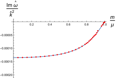
Figure 2: We depict the speed of zero sound (left) and the attenuation divided by momentum squared (right) for the D3-D5 intersection with $\hat{d}=10^{6}$ ($\hat{d}$, $\hat{\omega}$, and $\hat{k}$ are defined in (7.17) and (7.35)). The dots have been obtained by integrating numerically the fluctuation equations (A.48) and (A.49). The continuous line corresponds to the analytic expression (4.38).

In Fig. 2 we check (4.38) by comparing it with the results obtained by numerical integration at non-zero (but small) temperature. As it can be appreciated in this figure, the agreement is very good, both for the speed of zero sound $c_{s}$ and for the attenuation (i.e., the imaginary part of $\omega$).

4.4 The $p=4$ case

As pointed out around (4.8), the $p=4$ case is special and we have to modify our analysis. Indeed, the expansion of the Hankel function $H_{1}^{(1)}(x)$ near $x=0$ contains logarithmic terms, which implies that $E(\rho)$ and $\xi(\rho)$ behave near the horizon at low frequency as:

$$E(\rho) = A\,\rho+A\,c_{4}\,\Lambda^{2}\,+\,A\,\Lambda^{2}\,\log\big{(}{\rho\over\Lambda^{2}}\big{)}\,+\,\cdots$$

$$\xi(\rho) = B\,\rho+B\,c_{4}\,\Lambda^{2}\,+\,B\,\Lambda^{2}\,\log\big{(}{\rho\over\Lambda^{2}}\big{)}\,+\,\cdots\,\,,$$ (4.39)

where $c_{4}$ is the constant:

$$c_{4}=i\,\pi+1-2\gamma_{E}\,\,.$$ (4.40)

In (4.40) $\gamma_{E}=0.577\cdots$ is the Euler-Mascheroni constant. Let us now try to obtain the expansion (4.39) by performing the limits in the opposite order. As in [12], we have to compute the next correction to (4.17) and (4.19) near the horizon. First we notice that the equations satisfied by $E(\rho)$ and $\xi(\rho)$ near $\rho=0$ are just obtained by taking $p=4$ in (4.5):

$$E^{\prime\prime}\,=\,-{\Lambda^{2}\over\rho^{3}}\,\,E\,\,,\qquad\qquad\xi^{\prime\prime}\,=\,-{\Lambda^{2}\over\rho^{3}}\,\xi\,\,.$$ (4.41)

Neglecting the right-hand side in (4.41) and integrating twice, we arrive at a linear solution as in (4.17) and (4.19). To go beyond this approximation we plug the values of $E$ and $\xi$ into the right-hand side of (4.41) and perform the integration. In the low-frequency limit $\omega^{2}\ll\rho$, we have:

$$E(\rho) = E^{(0)}+b_{1}C_{1}+b_{2}C_{2}+(a_{1}C_{1}+a_{2}C_{2})\rho+(a_{1}C_{1}+a_{2}C_{2})\Lambda^{2}\log\rho+\cdots$$

$$\xi(\rho) = \ \xi^{(0)}+\tilde{b}_{1}C_{1}+\tilde{b}_{2}C_{2}+(\tilde{a}_{1}C_{1}+\tilde{a}_{2}C_{2})\rho+(\tilde{a}_{1}C_{1}+\tilde{a}_{2}C_{2})\Lambda^{2}\log\rho+\cdots\,\,.$$ (4.42)

Let us now match (4.39) and (4.42). By comparing the linear and logarithmic terms of these equations we arrive at the same values of $A$ and $B$ as those written in (4.21). Moreover, using these values of $A$ and $B$ and identifying the constant terms, we find the following matrix relation between $(E^{(0)},\xi^{(0)})$ and $(C_{1},C_{2})$:

$$\begin{pmatrix}E^{(0)}\\ \\ \xi^{(0)}\end{pmatrix}\,=\,\begin{pmatrix}\Lambda^{2}\,(c_{4}-\log\Lambda^{2})\,a_{1}\,-\,b_{1}&&&\Lambda^{2}\,(c_{4}-\log\Lambda^{2})\,a_{2}\,-\,b_{2}\\ {}&{}\\ \Lambda^{2}\,(c_{4}-\log\Lambda^{2})\,\tilde{a}_{1}\,-\,\tilde{b}_{1}&&&\Lambda^{2}\,(c_{4}-\log\Lambda^{2})\,\tilde{a}_{2}\,-\,\tilde{b}_{2}\end{pmatrix}\,\begin{pmatrix}C_{1}\\ \\ C_{2}\end{pmatrix}\,\,.$$ (4.43)

As in the $p<4$ case, the sources vanish non-trivially when the determinant of the matrix written in (4.43) is zero, namely:

$$(\,a_{1}\,\tilde{a}_{2}+a_{2}^{2}\,)\,\Lambda^{2}\,(c_{4}-\log\Lambda^{2})^{2}\,-\,(a_{1}\,\tilde{b}_{2}\,+\,\tilde{a}_{2}\,b_{1}\,+\,2\,a_{2}\,b_{2}\,)\,\Lambda^{2}\,(c_{4}-\log\Lambda^{2})$$

$$\qquad\qquad\qquad\qquad+\,b_{1}\,\tilde{b}_{2}\,+\,b_{2}^{2}\,=\,0\,\,.$$ (4.44)

Notice that (4.44) is obtained from (4.23) by taking $p=4$ and changing $c_{p}\to c_{4}-\log\Lambda^{2}$ on the latter. Using this observation it is straightforward to find the dispersion relation encoded in (4.44). At leading order in $\omega\sim k$ (4.44) reduces to (4.25), which means that the leading dispersion relation is just given by (4.29) and (4.30). Moreover, the next-to-leading contribution $\delta\omega$ is:

$$\delta\omega\,=\,-\,{\sqrt{2}\,\,\lambda\over\mu}\,\,(c_{4}-\log\Lambda^{2})\,{(1-{\bf m}^{2})^{{3\over 2}}\over(\lambda-2{\bf m}^{2})^{{5\over 2}}}\,\,k^{3}\,\,.$$ (4.45)

The imaginary part of $\delta\omega$ is easily deduced from (4.45):

$${\rm Im}\,\delta\omega\,=\,-{\pi\,\sqrt{2}\,\lambda\over\mu}\,{(1-{\bf m}^{2})^{{3\over 2}}\over(\lambda-2{\bf m}^{2})^{{5\over 2}}}\,\,k^{3}\,\,.$$ (4.46)

Notice that (4.46) is the same as in the first equation in (4.35) for $p=4$. Similarly, the real part of $\delta\omega$ can be written as:

$${\rm Re}\,\delta\omega\,=\,{\sqrt{2}\,\lambda\over\mu}\,\Bigg{[}2\gamma_{E}-1+\log\Bigg{(}2\,{(1-{\bf m}^{2})^{{3\over 2}}\over\lambda-2{\bf m}^{2}}\,k^{2}\Bigg{)}\Bigg{]}\,{(1-{\bf m}^{2})^{{3\over 2}}\over(\lambda-2{\bf m}^{2})^{{5\over 2}}}\,\,k^{3}\,\,.$$ (4.47)

4.5 The $\lambda=2$ case

For $\lambda=2$ the integral ${\cal J}_{1}(\rho)$, defined in (4.13), is not convergent and, therefore, the expressions written in (4.15) for $E(\rho)$ and $\xi(\rho)$ at low frequency are not correct. In order to obtain the solution of (4.12) for $\lambda=2$, let us define the integral $\bar{\cal J}_{1}(\rho)$ as:

$$\bar{\cal J}_{1}(\rho)\,\equiv\,\int_{\rho}^{\infty}\,d\bar{\rho}\Big{[}{\bar{\rho}^{2}\over(\bar{\rho}^{2}+d^{2}-c^{2})^{{3\over 2}}}-{1\over\bar{\rho}}\Big{]}={\rho\over\sqrt{\rho^{2}+d^{2}-c^{2}}}-1\,+\,\log{2\rho\over\sqrt{\rho^{2}+d^{2}-c^{2}}+\rho}\,\,.$$ (4.48)

Then, (4.12) for $\lambda=2$ can be integrated as:

$$E(\rho) = E^{(0)}\,-\,(\omega^{2}-k^{2})\,C_{1}\,[\bar{\cal J}_{1}(\rho)-\log\rho]\,-\,\Big{[}[(k^{2}-\omega^{2})\,c^{2}+\omega^{2}\,d^{2}\,]C_{1}-cd\,k\,C_{2}\Big{]}\,{\cal J}_{2}(\rho)$$

$$\xi(\rho) = \xi^{(0)}\,+\,C_{2}\,[\bar{\cal J}_{1}(\rho)-\log\rho]\,+\,d\big{[}d\,C_{2}-c\,k\,C_{1}\big{]}\,{\cal J}_{2}(\rho)\,\,,$$ (4.49)

where $E^{(0)}$ and $\xi^{(0)}$ are constants. When $\rho$ is very large the integrals $\bar{\cal J}_{1}(\rho)$ and ${\cal J}_{2}(\rho)$ vanish by construction and thus $E(\rho)$ and $\xi(\rho)$ behave at the UV as:

$$E(\rho) = E^{(0)}+(\omega^{2}-k^{2})\,C_{1}\,\log\rho\,+\,\cdots$$

$$\xi(\rho) = \xi^{(0)}-C_{2}\,\log\rho\,+\cdots\,\,,\qquad\qquad(\rho\to\infty)\,\,.$$ (4.50)

As argued in [35], when the logarithmic behavior displayed in (4.50) is present, the sources are identified with the coefficients of the logarithms, which should vanish. It is clear from the behavior of $\xi(\rho)$ in (4.50) that we must require that $C_{2}=0$. Moreover, the logarithmic term in $E(\rho)$ is absent either when $C_{1}=0$ or when:

$$\omega=\pm k\,\,.$$ (4.51)

If $C_{1}=C_{2}=0$ it follows from (4.49) that the functions $E(\rho)$ and $\xi(\rho)$ are constant and also the matching with the near-horizon results in (4.8) imply that both $E$ and $\xi$ must vanish. Therefore, the only non-trivial solution is given by the dispersion relation (4.51), which corresponds to a zero sound mode without dissipation and speed $c_{s}^{2}=1$. Notice that this result coincides with the value of the speed of first sound in (2.40) for $\lambda=2$. Moreover, when $C_{2}=0$ and $\omega^{2}=k^{2}$, eq. (4.49) reduces to:

$$E(\rho)\,=\,E^{(0)}\,-\,\omega^{2}\,d^{2}\,C_{1}\,{\cal J}_{2}(\rho)\,\,,\qquad\qquad\xi(\rho)\,=\,\xi^{(0)}\,-\,c\,d\,k\,C_{1}\,{\cal J}_{2}(\rho)\,\,.$$ (4.52)

Taking $\rho\to 0$ in (4.52) we can match this result with (4.8) and, as a consequence, we can show that $E^{(0)}$ and $\xi^{(0)}$ are related to the constant $C_{1}$ as:

$$E^{(0)} = C_{1}\,{d^{2}\over d^{2}-c^{2}}\,\omega^{2}\,+\,c_{p}\,C_{1}\,{d\over d^{2}-c^{2}}\,\omega^{{2(6-p)\over 5-p}}$$

$$\xi^{(0)} = C_{1}\,{c\,d\over d^{2}-c^{2}}\,k\,+\,c_{p}\,C_{1}\,{c\over d^{2}-c^{2}}\,k\,\omega^{{2\over 5-p}}\,\,.$$ (4.53)

Notice that (4.53) coincides with (4.22) when $\lambda=2$, $C_{2}=0$ and $\omega^{2}=k^{2}$. In particular, these relations imply that the ratio of $E^{(0)}$ and $\xi^{(0)}$ is given by:

$${E^{(0)}\over\xi^{(0)}}\,=\,{d\over c}\,k\,\,.$$ (4.54)

The analysis performed so far in this section is valid for $p<4$. When $p=4$ we have to go beyond the leading term in $\omega$, as in section 4.4, in order to match the logarithmic terms in the near-horizon expansion. It is easy to check that the $\lambda=2$ solution written above can be corrected to match the $\rho\to 0$ expansion in (4.39). The dispersion relation is still given by (4.51) and (4.53) continues to hold in this case.

5 Hyperscaling violation near the critical point

As already mentioned, the probe D-brane systems analyzed above undergo a quantum phase transition as $\mu\to m$ and the density $d$ vanishes. It was shown in [30] that the critical points of the D3-D7 and D3-D5 intersections are described by a non-relativistic scale invariant field theory exhibiting hyperscaling violation. In this section we extend these results to the case of non-conformal backgrounds (i.e., for $p\not=3$) and we compute the corresponding critical exponents.

Let us thus follow the approach of [30] and study the behavior of the system near the quantum critical point at $\mu=m$. Accordingly, we consider a chemical potential of the form:

$$\mu\,=\,m+\,\bar{\mu}\,\,,$$ (5.1)

where $\bar{\mu}$ is considered to be small. At leading order in $\bar{\mu}$ we can expand the different thermodynamic functions of (2.34), (2.36), and (2.29) as:

$$\Omega = -P\,\approx\,-{2^{{\lambda+6\over 4}}\over\lambda+2}\,\gamma^{-{\lambda\over 2}}\,{\cal N}\,\big{(}m\,\bar{\mu})^{{\lambda+2\over 4}}$$

$$\epsilon = f\,\approx\,2^{{\lambda-2\over 4}}\,\gamma^{-{\lambda\over 2}}\,{\cal N}\,\,m^{{\lambda+6\over 4}}\,\,\bar{\mu}^{{\lambda-2\over 4}}$$

$$d \approx 2^{{\lambda-2\over 4}}\,\gamma^{-{\lambda\over 2}}\,m^{{\lambda+2\over 4}}\,\,\bar{\mu}^{{\lambda-2\over 4}}\,\,.$$ (5.2)

where $f$ is the free energy density. The non-relativistic energy density $e$ is defined as in [30]:

$$e\,=\,\epsilon\,-\,\rho_{ch}\,m\,=\,\epsilon\,-\,{\cal N}\,d\,m\,\,,$$ (5.3)

where $\rho_{ch}\,=\,{\cal N}\,d$ is the physical charge density. By using (2.36) and (2.29) we get:

$$e\,=\,{\cal{N}}\,\gamma^{-{\lambda\over 2}}\,\big{(}\mu^{2}\,-\,m^{2}\big{)}^{{\lambda-2\over 4}}\,\Big{[}{\lambda\mu^{2}+2m^{2}\over\lambda+2}\,-\,\mu\,m\,\Big{]}\,\,.$$ (5.4)

Expanding at leading order in $\bar{\mu}$, we arrive at:

$$e\,\approx\,2^{{\lambda-2\over 4}}\,{\lambda-2\over\lambda+2}\,{\cal N}\,\gamma^{-{\lambda\over 2}}\,\big{(}m\bar{\mu}\big{)}^{{\lambda+2\over 4}}\,\,.$$ (5.5)

Comparing this result with the one for the pressure in (5.2), we obtain the following relation between $e$ and $P$:

$$e\,=\,{\lambda-2\over 4}\,\,P\,\,.$$ (5.6)

According to the analysis in [30], the relation between $e$ and $P$ at zero temperature near the quantum critical point is:

$$e\,=\,{n-\theta\over z}\,P\,\,,$$ (5.7)

where $\theta$ is the hyperscaling violation exponent and $z$ is the dynamical critical exponent. Eq. (5.7) is a consequence of the scaling dimensions of $e$, $P$, $\bar{\mu}$, and $d$, namely: $[e]=[P]=z+n-\theta$, $[\bar{\mu}]=z$, and $[d]=n-\theta$. Thus, in our case we have the following relation between $\theta$ and $z$:

$$\theta\,=\,n\,-\,{\lambda-2\over 4}\,z\,\,.$$ (5.8)

Notice that the relation (5.8) between $\theta$ and $z$ coincides with the ones found in [30] for the D3-D7 system (taking $n=3$ and $\lambda=6$) and for the D3-D5 intersection (taking $n=2$ and $\lambda=4$). In order to determine $z$ we look at the speed of sound (2.40) for $\mu\approx m$. At first-order in $\bar{\mu}$ it is given by:

$$u_{s}^{2}\,\approx\,{4\over\lambda-2}\,{\bar{\mu}\over m}\,\,,$$ (5.9)

and the corresponding dispersion relation is:

$$\omega\,\approx\,\sqrt{{4\over\lambda-2}\,{\bar{\mu}\over m}}\,\,k\,\,.$$ (5.10)

Matching the scaling dimensions of both sides of (5.10) as in [30], using that $[\omega]=z$ and $[k]=1$, we conclude that:

$$z\,=\,2\,\,.$$ (5.11)

Therefore $\theta$ takes the value:

$$\theta\,=\,n\,-\,{\lambda\over 2}\,+1\,\,.$$ (5.12)

Taking into account that for the SUSY D$p$-D$q$ intersections we are considering

$$n\,=\,{p+q-4\over 2}\,\,,\qquad\qquad\lambda\,=\,q-p+2\,\,,$$ (5.13)

we can rewrite the expression of $\theta$ simply as:

$$\theta\,=\,p\,-\,2\,\,.$$ (5.14)

Notice that for a D3-D$q$ intersection the previous formula gives $\theta=1$, in agreement with [30]. Eq. (5.14) is the generalization of this result for any $p$.

Let us now consider the system at finite temperature $T$. According to the analysis of [38], when $T$ is small the free energy density can be approximated as:

$$f(\mu,m,T)\,=\,f(\mu,m,T=0)\,+\,\pi\,\rho_{ch}\,T\,+\,{\mathcal{O}}(T^{2})\,\,.$$ (5.15)

Then, the non-relativistic free energy density is given by:

$$f_{non-rel}(\mu,m,T)\,=\,f(\mu,m,T)\,-\,\rho_{ch}\,m\,=\,e\,+\,\pi\,\rho_{ch}\,T\,+\,{\mathcal{O}}(T^{2})\,\,.$$ (5.16)

At leading order in $\bar{\mu}$ we have:

$$f_{non-rel}(\mu,m,T)\,=\,2^{{\lambda-2\over 4}}\,{\lambda-2\over\lambda+2}\,{\cal N}\,\gamma^{-{\lambda\over 2}}\,\big{(}m\bar{\mu}\big{)}^{{\lambda+2\over 4}}\,\Big{[}1\,+\,\pi\,{\lambda+2\over\lambda-2}\,{T\over\bar{\mu}}\,+\,{\mathcal{O}}\Big{(}\Big{(}{T\over\bar{\mu}}\Big{)}^{2}\Big{)}\Big{]}\,\,.$$ (5.17)

In the quantum critical region the non-relativistic free energy density should scale as:

$$f_{non-rel}\sim\big{(}\bar{\mu}\big{)}^{2-\alpha}\,g\Big{(}{T\over\bar{\mu}^{\nu z}}\Big{)}\,\,,$$ (5.18)

where $\alpha$ is the exponent which characterizes the scaling of the specific heat capacity $C$ and $\nu$ is the exponent corresponding to the correlation length $\xi$ (i.e., $C\sim(T-T_{c})^{-\alpha}$ and $\xi\sim(T-T_{c})^{-\nu}$ near a phase transition at $T=T_{c}$). Comparing (5.18) and (5.17) it follows that, in our case, we have:

$$2-\alpha\,=\,{\lambda+2\over 4}\,\,,\qquad\qquad\nu\,z\,=\,1\,\,.$$ (5.19)

Since $z=2$ for our system, the exponents $\alpha$ and $\nu$ are:

$$\alpha\,=\,{6-\lambda\over 4}\,\,,\qquad\qquad\nu\,=\,{1\over 2}\,\,.$$ (5.20)

Using the expression of $\lambda$ in terms of $p$ and $q$ written in (5.13), we can recast $\alpha$ simply as:

$$\alpha\,=\,1\,-\,{q-p\over 4}\,\,.$$ (5.21)

These results again coincide with the ones in [30] for the D3-D7 and D3-D5 intersections. Remarkably, the exponents obtained above satisfy the hyperscaling-violation relation:

$$(n+z-\theta)\,\nu\,=\,2-\alpha\,\,.$$ (5.22)

6 Zero sound in alternative quantization

In this section we will restrict ourselves to the study of intersections which are $(2+1)$-dimensional. In this case one can impose mixed Dirichlet-Neumann boundary conditions to the fluctuation modes, i.e., one can adopt an alternative quantization scheme [39, 40]. The equations of motion are the same for different quantizations, only the boundary conditions in the UV are different. On the dual field theory side this corresponds to having an anyonic fluid [31, 32, 33, 34]. Let us impose the following boundary condition at the UV:

$$\lim_{\rho\to\infty}\,\Big{[}\,\textfrak{n}\,\rho^{{\lambda\over 2}}\,f_{\rho\,\mu}\,-\,{1\over 2}\,\epsilon_{\mu\alpha\beta}\,f^{\alpha\beta}\,\big{]}\,=\,0\,\,,$$ (6.1)

where $\textfrak{n}$ is a constant that characterizes the boundary condition (the normal quantization condition considered so far corresponds to $\textfrak{n}=0$). As in [4], it is straightforward to prove that (6.1) is equivalent to require:

$$\lim_{\rho\to\infty}\,E\,=\,-i\,\textfrak{n}\,\lim_{\rho\to\infty}\,\big{[}\,\rho^{{\lambda\over 2}}\,a_{y}^{\prime}\,\big{]}\,\,,\qquad\qquad\lim_{\rho\to\infty}\,a_{y}\,=\,i\,{\textfrak{n}\over\omega^{2}-k^{2}}\,\lim_{\rho\to\infty}\,\big{[}\,\rho^{{\lambda\over 2}}\,E^{\prime}\,\big{]}\,\,.$$ (6.2)

Notice that, even if the equations of motion (3.13) and (3.14) for $E$ and $a_{y}$ are decoupled, the mixed boundary conditions (6.2) introduce a coupling between them. Therefore, to implement (6.2) we have to study the equation of motion of $a_{y}$, written in (3.14). Near the horizon $\rho\approx 0$ this equation reduces to:

$$a_{y}^{\prime\prime}\,+\,{\Lambda^{2}\over\rho^{7-p}}\,a_{y}\,=\,0\,\,,$$ (6.3)

which is just the same as (4.5). For $p<5$ the solution of (6.3) is given by the right-hand-side of (4.7). Moreover, for $p<4$ this solution behaves for low frequencies as:

$$a_{y}(\rho)\,=\,C\,\rho+C\,c_{p}\,\Lambda^{{2\over 5-p}}\,+\,\cdots\,\,,\qquad\qquad(p<4)\,\,,$$ (6.4)

with $C$ being a constant. We now perform the two limits in the opposite order. For low frequencies (3.14) reduces to:

$$\partial_{\rho}\,\Big{[}\sqrt{\rho^{\lambda}+d^{2}-c^{2}}\,a_{y}^{\prime}\Big{]}\,=\,0\,\,,$$ (6.5)

whose integration is straightforward:

$$a_{y}(\rho)\,=\,a_{y}^{(0)}\,-\,C_{3}\,{\cal J}_{3}(\rho)\,\,,$$ (6.6)

where $a_{y}^{(0)}=a_{y}(\rho\to\infty)$, $C_{3}$ is a constant of integration, and ${\cal J}_{3}(\rho)$ is the following integral (for $\lambda>2$):

$${\cal J}_{3}(\rho)\,=\,\int_{\rho}^{\infty}\,{d\bar{\rho}\over(\bar{\rho}^{\lambda}+d^{2}-c^{2})^{{1\over 2}}}\,=\,{2\over\lambda-2}\,\rho^{1-{\lambda\over 2}}\,F\Big{(}\,{1\over 2},{1\over 2}-{1\over\lambda};{3\over 2}\,-\,{1\over\lambda};-{d^{2}-c^{2}\over\rho^{\lambda}}\,\Big{)}\,\,.$$ (6.7)

Let us now expand $a_{y}(\rho)$ in powers of $\rho$. First, one can check that, for small $\rho$, the integral ${\cal J}_{3}(\rho)$ can be approximated as:

$${\cal J}_{3}(\rho)\,\approx\,{\mu\over d}\,-\,{\rho\over\sqrt{d^{2}-c^{2}}}\,\,,$$ (6.8)

where $\mu$ is the chemical potential (2.25). Therefore, for small $\rho$, $a_{y}$ can be approximated as:

$$a_{y}(\rho)\,\approx\,a_{y}^{(0)}\,-\,C_{3}\,{\mu\over d}\,+\,C_{3}\,{\rho\over\sqrt{d^{2}-c^{2}}}\,\,.$$ (6.9)

Let us now match (6.4) and (6.9). From the linear terms, we get the following relation between the constants $C$ and $C_{3}$:

$$C\,=\,{C_{3}\over\sqrt{d^{2}-c^{2}}}\,\,.$$ (6.10)

Using this relation, and identifying the constant terms in (6.4) and (6.9), we get the following relation between $a_{y}^{(0)}$ and $C_{3}$:

$$a_{y}^{(0)}\,=\,\Big{[}\,{\mu\over d}\,+\,{c_{p}\over\sqrt{d^{2}-c^{2}}}\,\Lambda^{{2\over 5-p}}\,\Big{]}\,C_{3}\,\,.$$ (6.11)

Let us now rewrite the boundary conditions (6.2) at low frequency and momentum. From the expressions of $E$ and $a_{y}$ in this regime (eqs. (4.12) and (6.6)), we conclude that they behave in the UV as:

$$E^{\prime}\big{|}_{\rho\to\infty}\approx(\omega^{2}-k^{2})\,\rho^{-{\lambda\over 2}}\,C_{1}\,\,,\qquad\qquad a_{y}^{\prime}\big{|}_{\rho\to\infty}\approx\rho^{-{\lambda\over 2}}\,C_{3}\,\,.$$ (6.12)

Taking this into account, we can recast the boundary conditions for the alternative quantization as a relation between the constants $E^{(0)}$, $a_{y}^{(0)}$, $C_{2}$, and $C_{3}$. Indeed, let us define $E_{\textfrak{n}}^{(0)}$ and $a_{y,\textfrak{n}}^{(0)}$ as:

$$E_{\textfrak{n}}^{(0)}\,\equiv E^{(0)}\,+\,i\,\textfrak{n}\,C_{3}\,\,,\qquad\qquad a_{y,\textfrak{n}}^{(0)}\,=\,a_{y}^{(0)}\,-\,i\,\textfrak{n}\,C_{1}\,\,.$$ (6.13)

Then, (6.2) is equivalent to the conditions:

$$E_{\textfrak{n}}^{(0)}\,=\,a_{y,\textfrak{n}}^{(0)}\,=\,0\,\,.$$ (6.14)

The UV values $E_{\textfrak{n}}^{(0)}$, $\xi^{(0)}$, and $a_{y,\textfrak{n}}^{(0)}$ can be related to the constants $C_{1}$, $C_{2}$, and $C_{3}$. In matrix form this relation becomes:

$$\begin{pmatrix}E_{\textfrak{n}}^{(0)}\\ \\ \xi^{(0)}\\ \\ a_{y,\textfrak{n}}^{(0)}\end{pmatrix}\,=\,\begin{pmatrix}\Lambda^{{2\over 5-p}}\,c_{p}\,a_{1}\,-\,b_{1}&&&\Lambda^{{2\over 5-p}}\,c_{p}\,a_{2}\,-\,b_{2}&&&i\,\textfrak{n}\\ {}&{}\\ \Lambda^{{2\over 5-p}}\,c_{p}\,\tilde{a}_{1}\,-\,\tilde{b}_{1}&&&\Lambda^{{2\over 5-p}}\,c_{p}\,\tilde{a}_{2}\,-\,\tilde{b}_{2}&&&0\\ {}&{}\\ -i\,\textfrak{n}&&&0&&&{\mu\over d}+{c_{p}\over\sqrt{d^{2}-c^{2}}}\,\Lambda^{{2\over 5-p}}\end{pmatrix}\,\begin{pmatrix}C_{1}\\ \\ C_{2}\\ \\ C_{3}\end{pmatrix}\,\,,$$ (6.15)

where $a_{1},a_{2},b_{1},b_{2}$ and $\tilde{a}_{1},\tilde{a}_{2},\tilde{b}_{1},\tilde{b}_{2}$ are given in (4.18) and (4.20), respectively. To have a non-trivial solution of the condition $E_{\textfrak{n}}^{(0)}=\xi^{(0)}=a_{y,\textfrak{n}}^{(0)}=0$ we must require that the determinant of the matrix in (6.15) be zero. This leads to:

$$\Big{(}\Big{[}\Lambda^{{2\over 5-p}}\,c_{p}\,a_{1}\,-\,b_{1}\Big{]}\Big{[}\Lambda^{{2\over 5-p}}\,c_{p}\,\tilde{a}_{2}\,-\,\tilde{b}_{2}\Big{]}-\Big{[}\Lambda^{{2\over 5-p}}\,c_{p}\,a_{2}\,-\,b_{2}\Big{]}\Big{[}\Lambda^{{2\over 5-p}}\,c_{p}\,\tilde{a}_{1}\,-\,\tilde{b}_{1}\Big{]}\Big{)}$$

$$\qquad\qquad\times\Big{[}{\mu\over d}+{c_{p}\over\sqrt{d^{2}-c^{2}}}\,\Lambda^{{2\over 5-p}}\Big{]}+\textfrak{n}^{2}\,\Big{[}\tilde{b}_{2}-\Lambda^{{2\over 5-p}}\,c_{p}\,\tilde{a}_{2}\Big{]}\,=\,0\,\,.$$ (6.16)

At leading order in frequency and momentum this equation simplifies as:

$$b_{1}\,\tilde{b}_{2}+b_{2}^{2}+{d\,\textfrak{n}^{2}\over\mu}\,\tilde{b}_{2}\,=\,0\,\,.$$ (6.17)

Since:

$$b_{1}\,\tilde{b}_{2}+b_{2}^{2}\,=\,{\gamma^{2}\over\lambda}\,\big{(}d^{2}-c^{2}\big{)}^{{2\over\lambda}-2}\,\Big{[}2(d^{2}-c^{2})\,k^{2}\,-\,(\lambda d^{2}-2c^{2})\,\omega_{0}^{2}\Big{]}\,\,,$$ (6.18)

then (6.17) implies the following gapped dispersion relation:

$$\omega^{2}\,=\,\omega^{2}_{0}\,=\,{2(d^{2}-c^{2})\over\lambda\,d^{2}-2\,c^{2}}\,k^{2}+\Big{(}{d\,\textfrak{n}\over\mu}\Big{)}^{2}\,\,.$$ (6.19)

In terms of the reduced mass parameter ${\bf m}$, defined in (4.27), we have

$$\omega^{2}_{0}\,=\,2\,\,{1-{\bf m}^{2}\over\lambda\,-2\,{\bf m}^{2}}\,k^{2}+\Big{(}{d\,\textfrak{n}\over\mu}\Big{)}^{2}\,\,.$$ (6.20)

One can also calculate the next order term in the dispersion relation. Indeed, one can check that $\omega=\omega_{0}+\delta\omega$, where $\delta\omega$ is given by:

$$\delta\omega\,=\,-\,2^{{p-3\over 2(5-p)}}\,c_{p}\,{\lambda\,\over\mu}\,{(1-{\bf m}^{2})^{{6-p\over 5-p}-{1\over 2}}\over(\lambda-2{\bf m}^{2})^{{7-p\over 2(5-p)}+1}}\,\,k^{{7-p\over 5-p}}\,\,\,-\,{\textfrak{n}^{2}\over\lambda-2}\,{c_{p}\over k\mu^{3}}\,\Big{(}{\gamma\over\mu}\Big{)}^{{\lambda\over 2}}\,{\omega_{0}^{{p-3\over 5-p}}\over(1-{\bf m}^{2})^{{1\over 2}+{\lambda\over 4}}}\,\,.$$ (6.21)

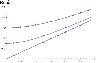
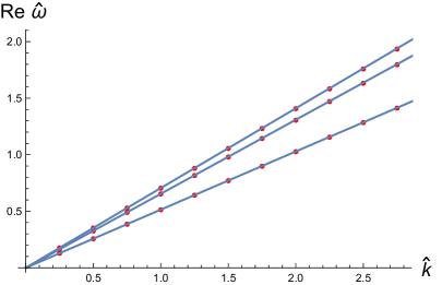
Figure 3: We plot the dispersions in the D3-D5 model $(p=3,\lambda=4)$ at $\hat{d}=10^{6}$ and $\hat{B}=3\cdot 10^{3}$. In both plots the red points stand for numerical results whereas the blue curves are the analytic from (6.23); we emphasize that the analytic result (6.23) is an educated guess, but reproduces the numerics precisely. (left) We vary the quantization parameter $\textfrak{n}=0,\frac{1}{2}\textfrak{n}_{crit},\textfrak{n}_{crit}$ (top-down) at fixed $\frac{m}{\mu}=0.5$. (right) The quantization parameter is chosen to be critical $\textfrak{n}=\textfrak{n}_{crit}$. Different lines correspond to varying $\frac{m}{\mu}=0.1,0.5,0.8$ (top-down).

It was noticed in [4] for the massless embeddings that the effect of the alternative quantization is equivalent to switching on a magnetic field traversing the $x^{1}x^{2}$ plane. Actually, it was found in [4] that the effect of a magnetic field $B$ effectively changes the parameter $\textfrak{n}$ as

$$\textfrak{n}\to\textfrak{n}-{B\over d}\,\,.$$ (6.22)

In the present massive case we cannot verify analytically the substitution rule (6.22) since the embedding function $z(\rho)$ is not a cyclic variable in the presence of a $B$ field. Therefore, we conjecture that the dispersion relation of the zero sound with general anyonic boundary conditions and magnetic field is given (at leading order) by:

$$\omega^{2}_{0}\,=\,2\,\,{1-{\bf m}^{2}\over\lambda\,-2\,{\bf m}^{2}}\,k^{2}+{1\over\mu^{2}}\,\big{(}d\,\textfrak{n}-B\big{)}^{2}\,\,.$$ (6.23)

Thus, the spectrum is generically gapped for non-vanishing $B$ and $\textfrak{n}$. However, it can be made gapless by adjusting the alternative quantization parameter $\textfrak{n}$ to the critical value:

$$\textfrak{n}_{crit}\equiv{B\over d}\,\,.$$ (6.24)

This particular case corresponds to one, where the anyonic fluid experiences zero net effective magnetic field, thus the resulting spectrum is also gapless. In Fig. 3 we compare the results obtained from the numerical integration of the fluctuation equations to our analytic formula (6.23). We see that the agreement is very good and, in particular, the numerics confirm that the spectrum becomes gapless at $\textfrak{n}=\textfrak{n}_{crit}$.

7 Finite temperature

Let us now consider the D$p$-D$q$ intersections $(n\,|\,p\perp q)$ at non-zero temperature and magnetic field. First, we introduce a more convenient system of coordinates. Let us represent the different components of the Cartesian coordinates $\vec{y}$ transverse to the D$p$-brane as:

$$y^{m}\,=\,r\,\cos\theta\,\eta^{m}\,\,,\qquad\qquad m=1,\cdots,q-n\,\,,$$

$$y^{l}\,=\,r\sin\theta\,\xi^{l}\,\,,\qquad\qquad\,\,\,\,\,\,l=q-n+1\,\cdots,9-p\,\,,$$ (7.1)

where $\eta^{m}$ and $\xi^{l}$ satisfy:

$$\sum_{m=1}^{q-n}\big{(}\eta^{m}\big{)}^{2}\,=\,\sum_{l=q-n+1}^{9-p}\big{(}\xi^{l}\big{)}^{2}\,=\,1\,\,.$$ (7.2)

Clearly, the $\eta^{m}$ ($\xi^{l}$) are the coordinates of a $(q-n-1)$-sphere ($(8+n-p-q)$-sphere). As:

$$\sum_{l=q-n+1}^{9-p}\big{(}y^{l}\big{)}^{2}\,=\,r^{2}\,\sin^{2}\theta\,\,,\qquad\qquad\sum_{m=1}^{q-n}\big{(}y^{m}\big{)}^{2}\,=\,r^{2}\,\cos^{2}\theta\,\,,$$ (7.3)

we identify the coordinates $z$ and $\rho$ used so far with:

$$z\,=\,r\,\sin\theta\,\,,\qquad\qquad\rho\,=\,r\,\cos\theta\,\,.$$ (7.4)

It is straightforward to check that

$$d\vec{y}\cdot d\vec{y}\,=\,dr^{2}\,+\,r^{2}\,\big{[}d\theta^{2}\,+\,\cos^{2}\theta\,d\Omega^{2}_{\parallel}\,+\,\sin^{2}\theta\,d\Omega^{2}_{\perp}\big{]}\,\,,$$ (7.5)

where $d\Omega^{2}_{\parallel}=d\Omega^{2}_{q-n-1}$ is the line element of the $(q-n-1)$-sphere of the D$q$-brane worldvolume and $d\Omega^{2}_{\perp}=d\Omega^{2}_{8+n-p-q}$ is the metric of the $(8+n-p-q)$-sphere transverse to the D$q$-brane. The ten-dimensional metric of a black D$p$-brane in these coordinates is:

$$ds^{2}_{10}=\Big{(}{r\over R}\Big{)}^{{7-p\over 2}}\big{[}-f_{p}(r)\,dt^{2}\,+\,d\vec{x}^{\,2}\big{]}+\Big{(}{R\over r}\Big{)}^{{7-p\over 2}}\Big{[}{dr^{2}\over f_{p}(r)}\,+\,r^{2}\big{(}d\theta^{2}+\cos^{2}\theta\,d\Omega^{2}_{\parallel}+\sin^{2}\theta\,d\Omega^{2}_{\perp}\big{)}\Big{]}\,\,,$$ (7.6)

where $R$ is a constant radius and the blackening factor $f_{p}$ is:

$$f_{p}(r)\,=\,1\,-\,\Big{(}{r_{h}\over r}\Big{)}^{7-p}\,\,,$$ (7.7)

and $r_{h}$ is the horizon radius, that is related to the temperature as follows:

$$T\,=\,{7-p\over 4\pi}\,r_{h}^{{5-p\over 2}}\,\,.$$ (7.8)

Let us consider a D$q$-brane probe extended along $t,x^{1}\ldots,x^{n},r$ and the $(q-n-1)$-sphere. If the brane is at a fixed point in the transverse sphere and we take $\theta=\theta(r)$, the induced metric is (for $R=1$):

$$ds^{2}_{q+1}\,=\,r^{{7-p\over 2}}\,\big{[}-f_{p}\,dt^{2}+(dx^{1})^{2}+\cdots+(dx^{n})^{2}\big{]}\,+\,r^{{p-7\over 2}}\,\big{[}(1+r^{2}\,f_{p}\,\dot{\theta}^{2}){dr^{2}\over f_{p}}+r^{2}\cos\theta^{2}\,d\Omega^{2}_{\parallel}\big{]}\,\,,$$ (7.9)

with $\dot{\theta}=d\theta/dr$. In what follows we will take $n$, $p$ and $q$ to be related as in (2.16). Moreover, we will add a magnetic field in the $x^{1}\,x^{2}$ directions. The Ansatz for the worldvolume gauge field strength in this case becomes:

$$F\,=\,\dot{A}_{t}\,dr\wedge dt\,+\,B\,dx^{1}\wedge dx^{2}\,\,.$$ (7.10)

The DBI Lagrangian density for this Ansatz is:

$${\cal L}\,=\,-{\cal N}\,\sqrt{H}\,(\cos\theta)^{{\lambda\over 2}}\,\sqrt{1-\dot{A}_{t}^{2}\,+\,r^{2}\,f_{p}\,\dot{\theta}^{2}}\,\,,$$ (7.11)

where $\lambda$ is given by (2.17) and we have introduced a new function $H$, defined as:

$$H\,\equiv\,r^{\lambda}\,+\,r^{\lambda+p-7}\,B^{2}\,\,.$$ (7.12)

In this Lagrangian $A_{t}$ is a cyclic variable. Its equation of motion can be integrated once to give:

$${(\cos\theta)^{{\lambda\over 2}}\,\sqrt{H}\,\dot{A}_{t}\over\sqrt{1-\dot{A}_{t}^{2}\,+\,r^{2}\,f_{p}\,\dot{\theta}^{2}}}\,=\,d\,\,,$$ (7.13)

with $d$ being an integration constant. From this last equation we obtain $\dot{A}_{t}$ as:

$$\dot{A}_{t}\,=\,d\,{\sqrt{1\,+\,r^{2}\,f_{p}\,\dot{\theta}^{2}}\over\sqrt{d^{2}+H\,\big{(}\cos\theta\big{)}^{\lambda}}}\,\,.$$ (7.14)

After eliminating $A_{t}$, we find the following equation for the embedding function $\theta(r)$:

$$\partial_{r}\,\Bigg{[}r^{2}\,f_{p}\,\sqrt{{d^{2}+H\,(\cos\theta)^{\lambda}\over 1\,+\,r^{2}\,f_{p}\,\dot{\theta}^{2}}}\,\,\dot{\theta}\Bigg{]}+{\lambda\over 2}\,H\,(\cos\theta)^{\lambda-1}\,\sin\theta\,{\sqrt{1\,+\,r^{2}\,f_{p}\,\dot{\theta}^{2}}\over\sqrt{d^{2}+H\,\big{(}\cos\theta\big{)}^{\lambda}}}\,=\,0\,\,.$$ (7.15)

The equation of motion (7.15) has explicit dependence on the blackening factor $f_{p}$, which has factors of the horizon radius $r_{h}$. This feeds in temperature dependence via (7.8). The horizon radius $r_{h}$ can be scaled out by an appropriate change of variables, followed by a redefinition of the density $d$ and the magnetic field $B$. Indeed, let us define the reduced radial variable $\hat{r}$ as follows:

$$\hat{r}\,=\,{r\over r_{h}}\,\,.$$ (7.16)

It is then straightforward to verify that, in terms of $\hat{r}$, the embedding equation is just (7.15) with $r_{h}=1$ and $d$ and $B$ substituted by the scaled quantities $\hat{d}$ and $\hat{B}$, defined as:

$$\hat{d}\,=\,{d\over r_{h}^{{\lambda\over 2}}}\,\,,\qquad\qquad\hat{B}\,=\,{B\over r_{h}^{{7-p\over 2}}}\,\,.$$ (7.17)

We will integrate (7.15) by imposing that the D$q$-brane intersects the horizon $r=r_{h}$ at some value $\theta_{h}\equiv\theta(r=r_{h})$, i.e., we will require that our embedding is a black hole embedding. At the UV $r\to\infty$ the function $\theta(r)$ behaves generically as:

$$\theta(r)\sim{m\over r}\,+\,{{\cal C}\over r^{{\lambda\over 2}}}\,+\,\cdots\,=\,{\hat{m}\over\hat{r}}\,+\,{\hat{\cal C}\over\hat{r}^{{\lambda\over 2}}}\,+\,\cdots\qquad\qquad(r\to\infty)\,\,,$$ (7.18)

where $m$ and ${\cal C}$ are related to the mass and condensate, respectively. Notice that we have introduced in (7.18) the scaled quantities $\hat{m}$ and $\hat{\cal C}$, related to $m$ and ${\cal C}$ as:

$$\hat{m}\,=\,{m\over r_{h}}\,\,,\qquad\qquad{\hat{\cal C}}\,=\,{{\cal C}\over r_{h}^{{\lambda\over 2}}}\,\,.$$ (7.19)

It is also interesting to write the chemical potential $\mu$ in terms of the scaled quantities. We have:

$$\hat{\mu}\,=\,{\mu\over r_{h}}\,\,,$$ (7.20)

where $\hat{\mu}$ is given by the following integral:

$$\hat{\mu}\,=\,\hat{d}\,\int_{1}^{\infty}d\hat{r}{\sqrt{1+\hat{r}^{p-5}\,(\hat{r}^{7-p}-1)\,\big{(}{d\theta\over d\hat{r}}\big{)}^{2}}\over\sqrt{\hat{d}^{2}+(\hat{r}^{\lambda}+\hat{r}^{\lambda+p-7}\hat{B}^{2})(\cos\theta)^{\lambda}}}\,\,.$$ (7.21)

Notice that $\hat{m}/\hat{\mu}=m/\mu$, i.e., the horizon radius $r_{h}$ drops out when one computes the mass/chemical potential ratio as both of the quantities have the same dimension.

7.1 Charge susceptibility

Let us consider now the case $B=0$ and compute the charge susceptibility $\chi$, which is defined as:

$$\chi\,=\,{\partial\rho_{ch}\over\partial\mu}\,\,.$$ (7.22)

Taking into account that the charge density $\rho_{ch}$ is related to $d$ as $\rho_{ch}\,=\,{\cal N}\,d$, we can rewrite the last expression as:

$$\chi^{-1}\,=\,{1\over{\cal N}}\,{\partial\mu\over\partial d}=\frac{1}{{\cal N}}\int_{r_{h}}^{\infty}\,{\partial\dot{A}_{t}\over\partial d}\,dr\,\,.$$ (7.23)

By a direct calculation using (7.14) for $B=0$ , we get:

$${\partial\dot{A}_{t}\over\partial d}\,=\,\sqrt{\Delta}\,{r^{{\lambda\over 2}}\,\big{(}\cos\theta\big{)}^{{\lambda\over 2}}\over d^{2}+r^{\lambda}\,\big{(}\cos\theta\big{)}^{\lambda}}\,\Bigg{[}1+d\Bigg{(}{\lambda\over 2}\,\tan\theta\,{\partial\theta\over\partial d}\,+\,{r^{2}\,f_{p}\,\dot{\theta}\over\Delta}\,{\partial\dot{\theta}\over\partial d}\Bigg{)}\Bigg{]}\,\,,$$ (7.24)

where $\Delta$ is defined as:

$$\Delta\,\equiv\,1-\dot{A}_{t}^{2}+r^{2}\,f_{p}\,\dot{\theta}^{2}\,=\,r^{\lambda}\,(\cos\theta)^{\lambda}\,{1+r^{2}\,\,f_{p}\,\dot{\theta}^{2}\over d^{2}+r^{\lambda}\,(\cos\theta)^{\lambda}}\,\,.$$ (7.25)

Therefore, the charge susceptibility can be written as:

$$\chi^{-1}\,=\,{1\over{\cal N}}\,\int_{r_{h}}^{\infty}\,dr\,\sqrt{\Delta}\,{r^{{\lambda\over 2}}\,\big{(}\cos\theta\big{)}^{{\lambda\over 2}}\over d^{2}+r^{\lambda}\,\big{(}\cos\theta\big{)}^{\lambda}}\,\Bigg{[}1+d\Bigg{(}{\lambda\over 2}\,\tan\theta\,{\partial\theta\over\partial d}\,+\,{r^{2}\,f_{p}\,\dot{\theta}\over\Delta}\,{\partial\dot{\theta}\over\partial d}\Bigg{)}\Bigg{]}\,\,.$$ (7.26)

Let us consider some particular cases of (7.26). First of all, we consider the massless case, in which $\theta=0$ and the integral in (7.26) can be performed explicitly. We get:

$${\cal N}\,\chi^{-1}\,=\,{2\over\lambda-2}\,r_{h}^{1-{\lambda\over 2}}\,F\Big{(}{3\over 2},{1\over 2}-{1\over\lambda};{3\over 2}\,-\,{1\over\lambda};-{d^{2}\over r_{h}^{\lambda}}\Big{)}\ ,\ \ m=0\ .$$ (7.27)

Another interesting limiting case is when $T=0$ . In this case we can obtain $\chi$ without using (7.26). Indeed, we can compute the derivative of $\mu$ from the second equation in (2.29). Computing $\partial d/\partial\mu$ for constant $m$, we get:

$${\partial d\over\partial\mu}\,=\,\gamma^{-{\lambda\over 2}}\,\big{(}\mu^{2}-m^{2}\big{)}^{{\lambda-6\over 4}}\,\Big{[}{\lambda\over 2}\,\mu^{2}\,-\,m^{2}\Big{]}\ ,\ \ T=0\ ,$$ (7.28)

where $\gamma$ is the constant defined in (2.26). Then, it follows that:

$$\chi\,=\,{\cal N}\,\gamma^{-{\lambda\over 2}}\,{{\lambda\over 2}\,\mu^{2}\,-\,m^{2}\over\big{(}\mu^{2}-m^{2}\big{)}^{{6-\lambda\over 4}}}\ \ ,\ T=0\ .$$ (7.29)

Notice that (for $\lambda<6$), the zero temperature susceptibility blows up when $m=\mu$.

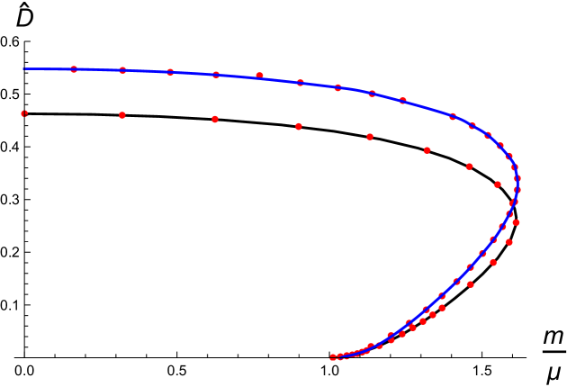
Figure 4: We plot the rescaled diffusion constant $\hat{D}\,=\,r_{h}^{{5-p\over 2}}\,D$ for the D2-D6 model at $\hat{d}=1$. The solid blue curve is obtained purely from the background for $\hat{B}=0$, i.e., by evaluating the integral (7.31). The red points, on the other hand, are numerical results from the fluctuation analysis by solving the coupled equations of motion in (A.48)-(A.50) for zero magnetic field. We see that the two different methods agree perfectly. The lower black curve is the result obtained from (7.42) for $\hat{B}=1/2$, while the red points are the result of the numerical integration of the fluctuation equations for this value of $\hat{B}$. Again, both methods agree perfectly.

7.2 Einstein relation

The diffusion constant $D$ can be related to the charge susceptibility $\chi$ by means of the so-called Einstein relation, which reads:

$$D\,=\,\sigma\,\chi^{-{1}}\,\,,$$ (7.30)

where $\sigma$ is the DC conductivity. The value of $\sigma$ can be extracted from the analysis of the two-point correlators of the transverse currents. This analysis is carried out in appendix B. The final result for $\sigma$ is written in (B.34). Plugging this value of $\sigma$ and the susceptibility written in (7.26) into (7.30), we arrive at the following expression for $D$:

$$D\,=\,r_{h}^{{p-7\over 2}}\,\sqrt{r_{h}^{\lambda}(\cos\theta_{h})^{\lambda}+d^{2}}\,\int_{r_{h}}^{\infty}\,dr\,\sqrt{\Delta}\,{r^{{\lambda\over 2}}\,\big{(}\cos\theta\big{)}^{{\lambda\over 2}}\over d^{2}+r^{\lambda}\,\big{(}\cos\theta\big{)}^{\lambda}}$$

$$\qquad\qquad\qquad\qquad\times\Bigg{[}1+d\Bigg{(}{\lambda\over 2}\,\tan\theta\,{\partial\theta\over\partial d}\,+\,{r^{2}\,f_{p}\,\dot{\theta}\over\Delta}\,{\partial\dot{\theta}\over\partial d}\Bigg{)}\Bigg{]}\,\,.$$ (7.31)

Let us now extract the low temperature behavior of $D$ by using the $T=0$ susceptibility written in (7.29). As $\sigma\sim{\cal N}\,d\,r_{h}^{{p-7\over 2}}$ for low $T$, we get:

$$D\approx 2\,\gamma^{{\lambda\over 2}}\,{\big{(}\mu^{2}-m^{2}\big{)}^{{6-\lambda\over 4}}\over\lambda\,\mu^{2}-2\,m^{2}}\,\,d\,r_{h}^{{p-7\over 2}}\,\,\,,\qquad\qquad\quad(T\sim 0).$$ (7.32)

The expression (7.31) for $D$ can be compared with the values obtained by analyzing the spectrum of diffusive modes of the probe in the hydrodynamical regime (see section 7.3 below). This comparison is shown in Fig. 4 for the D2-D6 intersection. We have obtained a very good agreement between the two methods in all intersections studied.

7.3 Fluctuations

Let us now consider a fluctuation of the embedding angle and of the gauge field of the form:

$$\theta(x^{\mu},r)\,=\,\theta_{0}(r)+\zeta(x^{\mu},r)\,\,,\qquad\qquad A(x^{\mu},r)\,=\,A^{(0)}(r)\,+\,a(x^{\mu},r)\,\,,$$ (7.33)

where $a(x^{\mu},r)=a_{\nu}(x^{\mu},r)dx^{\nu}$ and $A^{(0)}=A_{\nu}^{(0)}\,dx^{\nu}=A_{t}\,dt+B\,x^{1}\,dx^{2}$ is the one-form for the unperturbed gauge field. We will choose the gauge in which $a_{r}=0$ and we will consider fluctuation fields $a_{\nu}$ and $\zeta$ depending only on $r$, $t$, and $x^{1}$. In this case it is possible to restrict to the case in which $a_{\nu}\not=0$ only when $\nu=t$, $x^{1}\equiv x$, and $x^{2}\equiv y$. In appendix A.2 we obtain the Lagrangian density for the fluctuations and we perform a detailed analysis of the corresponding equations of motion. This analysis is performed in momentum space. Accordingly, let us Fourier transform $a_{\nu}$ and $\zeta$ as:

$$a_{\nu}(r,t,x) = \int{d\omega\,dk\over(2\pi)^{2}}\,a_{\nu}(r,\omega,k)\,e^{-i\omega\,t\,+\,ikx}$$

$$\zeta(r,t,x) = \int{d\omega\,dk\over(2\pi)^{2}}\,\zeta(r,\omega,k)\,e^{-i\omega\,t\,+\,ikx}\,\,.$$ (7.34)

At very low temperature the numerical analysis of the coupled fluctuation equations (A.48), (A.49), and (A.50) allows to find sound modes, i.e., the zero sound. The corresponding dispersion relation is given in terms of the rescaled frequency and momentum $\hat{\omega}$ and $\hat{k}$, related to $\omega$ and $k$ as:

$$\hat{\omega}\,=\,{\omega\over r_{h}^{{5-p\over 2}}}\,\,,\qquad\qquad\hat{k}\,=\,{k\over r_{h}^{{5-p\over 2}}}\,\,.$$ (7.35)

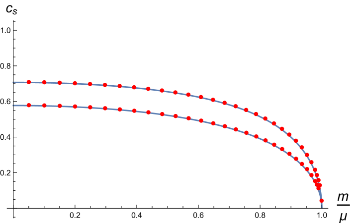
Figure 5: We demonstrate how well the analytics and numerics match also for the non-conformal brane intersections, by focusing on $p=2$ and at low temperature and vanishing magnetic field. We depict the speed of zero sound for two intersections D2-D4 ($\lambda=4$) and D2-D6 ($\lambda=6$) at $\hat{d}=10^{\lambda}$. The numerics are represented by red points whereas the analytics, following (4.30), are continuous curves. Lower dataset is for $\lambda=6$ and higher for $\lambda=4$. In extracting the slope we kept $\frac{\hat{k}}{\hat{d}^{\frac{5-p}{\lambda}}}=0.01$.

For vanishing magnetic field the numerical results are in very good agreement with the analytic equations of section 4, as it was illustrated already in Fig. 2 for the conformal D3-D5 intersection. This agreement is confirmed in Fig. 5 for the non-conformal cases D2-D4 and D2-D6.

At higher temperatures the system is in a hydrodynamic regime, in which the dominant mode is a diffusion mode with purely imaginary frequency. The spectrum of these diffusion modes can be written in terms of the rescaled frequency and momentum defined in (7.35) as:

$$\hat{\omega}\,=\,-i\,\hat{D}\,\hat{k}^{2}\,\,,$$ (7.36)

where $\hat{D}$ is the rescaled diffusion constant, related to $D$ as:

$$\hat{D}\,=\,r_{h}^{{5-p\over 2}}\,D\,\,.$$ (7.37)

The value of $\hat{D}$ predicted by Einstein relation can be straightforwardly obtained from (7.31). Indeed, one must simply take $r_{h}=1$ and change $d$ by $\hat{d}$ in (7.31). The low temperature limit of $\hat{D}$ can also be obtained easily from (7.32). We get:

$$\hat{D}\approx 2\,\gamma^{{\lambda\over 2}}\,{\big{(}\hat{\mu}^{2}-\hat{m}^{2}\big{)}^{{6-\lambda\over 4}}\over\lambda\,\hat{\mu}^{2}-2\,\hat{m}^{2}}\,\,\hat{d}\,\,\,,\qquad\qquad\qquad(T\sim 0).$$ (7.38)

In Fig. 6 we show the temperature dependence of $\hat{D}$ for the D2-D6 model. The temperature is decreased by increasing $\hat{d}$. The results displayed in Fig. 6 indeed show that $\hat{D}$ approaches the value written in (7.38) as $\hat{d}\to\infty$.

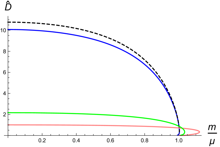
Figure 6: We depict the diffusion constant at various temperatures and vanishing magnetic field for the D2-D6 model $(p=2,\lambda=6)$ as obtained by solving the fluctuation equations. The continuous curves correspond to $\hat{d}=10^{1},10^{2},10^{4}$ (bottom-up). As a reference we have also included the $T\to 0$ analytic result (7.38) for $\hat{d}=10^{4}$, depicted as a dashed black curve, showing how well the $\hat{d}=10^{4}$ numerical curve is converging to it. Higher values of $\hat{d}$ would be overlapping even more.

Let us now consider the dependence on the magnetic field. The results of section 6 (and those of refs. [9, 10, 4]) strongly suggest that the spectrum of the zero sound is gapped and that the gap is just $B/\mu$. Therefore we are led to conjecture the following expression of the leading order dispersion relation of the zero sound:

$$\omega^{2}_{0}\,=\,2\,\,{1-{\bf m}^{2}\over\lambda\,-2\,{\bf m}^{2}}\,k^{2}+{B^{2}\over\mu^{2}}\,\,,$$ (7.39)

where we have just added the gap to the gapless value of $\omega_{0}^{2}$. Notice that (7.39) implies that the gap is independent of the quark mass $m$ for fixed chemical potential $\mu$. We have explicitly verified this feature numerically in Fig. 7 for the D2-D6 system.

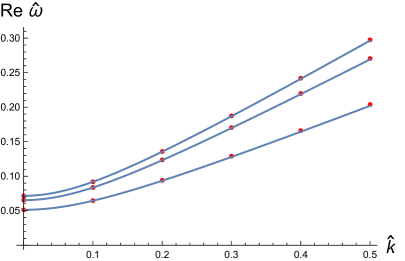
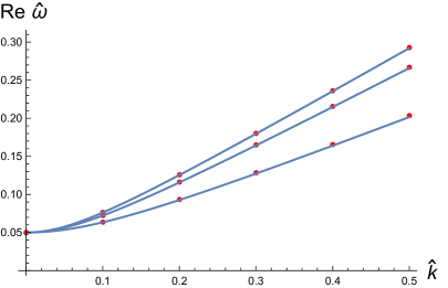
Figure 7: We present numerical evidence that our conjecture for the dispersions at low temperature (7.39) is supported at finite magnetic field strength. We demonstrate this in the case of the D2-D6 model ($p=2$,$\lambda=6$) at $\hat{B}=10$ for two different cases: in the canonical and in the grand canonical ensemble. From the latter case we clearly find that the mass gap of the zero sound is indeed independent of the mass ($\hat{m}$) of the fundamentals. Different curves in both panels correspond to $\frac{m}{\mu}=0.1,0.5,0.8$ (top-down). (Left) We keep the charge density fixed $\hat{d}=10^{6}$. (Right) We keep the chemical potential fixed $\hat{\mu}=200$.

Let us next analyze the dependence of the diffusion constant on the magnetic field $B$. In order to write the expression of $D$ which follows from the Einstein relation, we need to know the value of the DC conductivity $\sigma$ when $B\not=0$. In principle, this conductivity could be obtained from the analysis of the transverse correlators, as was done in appendix B for $B=0$. However, the fluctuation equations couple the transverse and longitudinal modes when $B\not=0$ and and it is not clear to us how to deal with this coupling. For this reason we we have computed $\sigma$ by applying the method of ref. [41]. The details of this calculation are explained in appendix C. The final result for $\sigma$ is:

$$\sigma\,=\,{\cal N}\,{\sqrt{r_{h}^{\lambda}(1+r_{h}^{p-7}\,B^{2})\,(\cos\theta_{h})^{\lambda}\,+d^{2}}\over r_{h}^{7-p}\,+\,B^{2}}\,\,r_{h}^{{7-p\over 2}}\,\,.$$ (7.40)

It is now straightforward to write down the expression of $D$ which follows from (7.30). Indeed, let us define $\Delta_{B}$ as:

$$\Delta_{B}\,=\,{H\,(\cos\theta)^{\lambda}\,(1+r^{2}\,f_{p}\,\dot{\theta}^{2})\over d^{2}+H\,(\cos\theta)^{\lambda}}\,\,,$$ (7.41)

where $H$ is the quantity defined in (7.12). Then, the Einstein relation gives the following value of the diffusion constant:

$$D\,=\,{\sqrt{r_{h}^{\lambda}(1+r_{h}^{p-7}\,B^{2})\,(\cos\theta_{h})^{\lambda}\,+d^{2}}\over r_{h}^{{7-p\over 2}}\,+\,r_{h}^{{p-7\over 2}}\,B^{2}}\,\,\int_{r_{h}}^{\infty}\,dr\,\sqrt{\Delta_{B}}\,{H\,\big{(}\cos\theta\big{)}^{{\lambda\over 2}}\over d^{2}+H\,\big{(}\cos\theta\big{)}^{\lambda}}$$

$$\qquad\qquad\qquad\qquad\times\Bigg{[}1+d\Bigg{(}{\lambda\over 2}\,\tan\theta\,{\partial\theta\over\partial d}\,+\,{r^{2}\,f_{p}\,\dot{\theta}\over\Delta_{B}}\,{\partial\dot{\theta}\over\partial d}\Bigg{)}\Bigg{]}\,\,.$$ (7.42)

In Fig. 4 we compare the predictions of (7.42) for the D2-D6 model and the numerical results obtained by direct integration of the coupled fluctuation equations (A.48)-(A.50). As can be appreciated in this figure, the agreement between the two methods is very good.

8 Summary and conclusions

In this paper we studied the collective excitations of flavor D$q$-branes in the supergravity background generated by color D$p$-branes. The two set of branes are separated in their transverse directions, which corresponds to adding massive flavors in the dual field theory. We first studied this D$p$-D$q$ model at $T=0$ and $\mu\not=0$ in the quenched approximation. The non-zero chemical potential is generated by a suitable worldvolume gauge field on the probe. We then generalized these results for $T\not=0$ and non-vanishing magnetic field.

At zero temperature and non-vanishing chemical potential the supersymmetric D$p$-D$q$ intersections with #ND=4 can be studied analytically. We obtained their thermodynamics and first and zero sound, generalizing previous results in the literature for the conformal cases with $p=3$. These results allow to characterize the quantum phase transition that occurs when $\mu=m$ and $d=0$. In this point several thermodynamic quantities vanish and the system displays a non-relativistic scaling behavior with hyperscaling violation. We have been able to compute the corresponding critical exponents.

We also analyzed the massive flavor brane systems at non-zero temperature and magnetic field. We verified numerically that, when the magnetic field is non-vanishing, the zero sound spectrum becomes gapped, with the gap given by $B/\mu$. Moreover, when $T$ is large enough the system enters into a hydrodynamic regime, which is dominated by a diffusion mode. We determined numerically the corresponding diffusion constant and verified the validity of the Einstein relation.

When the intersection is $(2+1)$-dimensional we performed an alternative quantization of the fluctuations, which corresponds to adding degrees of freedom with fractional statistics (anyons). In those systems the zero sound is generically gapped, although it becomes gapless if the magnetic field is chosen appropriately. In fact, this choice corresponds to a fluid of anyons experiencing zero effective magnetic field, thus the occurrence of gapless mode was expected. Our understanding of the anyonic fluid is still lacking, though. In order to describe its properties better one would need to make a definite choice for the $SL(2,\mathbb{Z})$ transformation as this is needed to make an identification of the resulting charge density of the anyons. Moreover, as there is a residual gauge freedom in adding boundary terms to the action, the calculation of the free energy depends crucially on the chosen $SL(2,\mathbb{Z})$ transformation. The variational principle is still well-defined, which allowed us in the current analysis to investigate the transport properties and collective phenomena of the anyon fluid in terms of the statistics, proportional to the quantization parameter $\mathfrak{n}$.

There are several other open topics which deserve further investigation. The D$p$-brane metrics with $p\not=3$ violate hyperscaling [42] with $\theta=-(p-3)^{2}/(5-p)$. It would be worth to explore the relation between this scaling of the background and the one found above for the probe. Another interesting problem for the future would be the analysis of more general D$p$-D$q$ intersections. Contrary to the supersymmetric cases studied here, the massive embeddings of a general D$p$-D$q$ model are generically unstable and one must turn on fluxes on the worldvolume of the probe to stabilize them (see, for example [43, 44, 45]). These additional worldvolume gauge fields give an important contribution to the Wess-Zumino term of the probe action. It would be very interesting to develop a general formalism for the collective excitations of the probe brane which could incorporate all the particular cases studied in the literature.

It would also be interesting to analyze the systems in which the backgrounds are not generated by branes in flat space. Let us mention the cases of branes on the conifold (as in the Klebanov-Witten model [48]) and the ABJM model [49]. Since the massive embeddings depend on the particular model, it is expected that the results will not be completely universal. It is interesting, however, to determine the features common to all the cases.

The collective excitations of brane intersections analyzed so far in the literature have been carried out in the probe approximation. Therefore, it is quite natural to explore the effects on the results of having dynamical quarks. In order to provide an answer to this problem we need to have supergravity backgrounds which include the backreaction of the flavor branes. By employing different approximations, these backgrounds can be found for some systems. Let us mention the case of ABJM with smeared flavor branes [50, 51, 52, 53], which are geometries free of pathologies, although they do not incorporate the effect of non-zero density. This effect is included in the geometry recently found in [54], which is dual to three-dimensional super Yang-Mills theory with compressible matter. In the near future we intend to study the collective excitations of the flavor branes for some of these systems.

Acknowledgments We thank Yago Bea and Carlos Hoyos for discussions and critical readings of the manuscript. N.J. is supported by the Academy of Finland grant no. 1268023. A. V. R. and G. I. are funded by the Spanish grant FPA2014-52218-P, by the Consolider-Ingenio 2010 Programme CPAN (CSD2007-00042), by Xunta de Galicia (GRC2013-024), and by FEDER. G. I. is also funded by FPA2012-35043-C02-02.

Appendix A Fluctuation equations of motion

In this appendix we obtain the Lagrangian density, and the corresponding equations of motion, for the fluctuations of the embedding scalar and the gauge fields at non-vanishing charge density $d\neq 0$ and magnetic field $B\neq 0$. As was the case for the background equations, it is useful to treat the analysis for $T=0$ and $T\neq 0$ using different parametrization.

A.1 Fluctuations at zero temperature

In this subsection we focus on $T=0$ case. Let us consider a fluctuation of the gauge field and embedding as in (3.1) and (3.2). The induced metric $g$ takes the form:

$$g\,=\,\bar{g}\,+\,\hat{g}\,\,,$$ (A.1)

where $\bar{g}$ is the zeroth-order metric and $\hat{g}$ is the perturbation. Let us split $\hat{g}$ in the form:

$$\hat{g}\,=\,\hat{g}^{(1)}\,+\,\hat{g}^{(2)}\,\,.$$ (A.2)

The non-zero elements of $\hat{g}^{(1)}$ are:

$$\hat{g}^{(1)}_{\rho x^{\mu}}\,=\,{z_{0}^{\prime}\over r^{{7-p\over 2}}}\,\partial_{\mu}\xi\,\,,\qquad\qquad\hat{g}^{(1)}_{\rho\rho}\,=\,{2\,z_{0}^{\prime}\over r^{{7-p\over 2}}}\,\partial_{\rho}\xi\,,$$ (A.3)

whereas $\hat{g}^{(2)}$ has the form:

$$\hat{g}^{(2)}_{ab}\,=\,{1\over r^{{7-p\over 2}}}\,\partial_{a}\xi\,\partial_{b}\xi\,\,.$$ (A.4)

(we are taking the radius $R=1$ in (2.14)). In order to expand the DBI D$q$-brane action we notice that the Born-Infeld determinant can be written as:

$$\sqrt{-\det(g+F)}\,=\,\sqrt{-\det\big{(}\,\bar{g}\,+\,{F^{(0)}}\,\big{)}}\,\sqrt{\det(1+X)}\,\,,$$ (A.5)

where the matrix $X$ is given by:

$$X\,\equiv\,\big{(}\,\bar{g}\,+\,F^{(0)}\,\big{)}^{-1}\,\,\big{(}\,\hat{g}\,+\,{f}\,\big{)}\,\,.$$ (A.6)

To evaluate the right-hand side of eq. (A.5), we shall use the expansion:

$$\sqrt{\det(1+X)}\,=\,1\,+\,{1\over 2}\,{\rm Tr}X\,-\,{1\over 4}\,{\rm Tr}X^{2}\,+\,{1\over 8}\,\big{(}{\rm Tr}X\big{)}^{2}\,+\,{\cal O}(X^{3})\,\,.$$ (A.7)

Moreover, in the inverse matrix $\big{(}\,\bar{g}\,+\,F^{(0)}\,\big{)}^{-1}$ we will separate the symmetric and antisymmetric parts:

$$\Big{(}\,\bar{g}\,+\,F^{(0)}\Big{)}^{-1}\,=\,{\cal G}^{-1}\,+\,{\cal J}\,\,,$$ (A.8)

where ${\cal J}$ is the antisymmetric component and the symmetric matrix ${\cal G}$ is the open string metric. The relevant components of ${\cal G}$ are:

$${\cal G}^{tt} = -{\bar{g}_{rr}\,(1+z_{0}^{\prime 2})\over\bar{g}_{rr}\,|\bar{g}_{tt}|(1+z_{0}^{\prime 2})\,-\,A_{t}^{(0)^{\prime}2}}\,\,,\qquad\qquad{\cal G}^{x^{i}\,x^{j}}\,=\,{\delta^{ij}\over\bar{g}_{xx}}$$

$${\cal G}^{\rho\rho} = -{\bar{g}_{tt}\over\bar{g}_{rr}\,|\bar{g}_{tt}|(1+z_{0}^{\prime 2})\,-\,A_{t}^{(0)^{\prime}2}}\,\,.$$ (A.9)

Using the fact that $\bar{g}_{rr}\,|\bar{g}_{tt}|=1$, and eliminating $z_{0}^{\prime}$ and $A_{t}^{(0)^{\prime}}$, we get:

$${\cal G}^{tt} = -{\rho^{\lambda}+d^{2}\over|\bar{g}_{tt}|\,\rho^{\lambda}}\,=\,-{\rho^{\lambda}+d^{2}\over(\rho^{2}+z_{0}^{2})^{{7-p\over 4}}\,\rho^{\lambda}}$$

$${\cal G}^{\rho\rho} = {\rho^{\lambda}+d^{2}-c^{2}\over\bar{g}_{rr}\,\rho^{\lambda}}\,=\,(\rho^{2}+z_{0}^{2})^{{7-p\over 4}}\,\,{\rho^{\lambda}+d^{2}-c^{2}\over\rho^{\lambda}}$$

$${\cal G}^{x^{i}\,x^{j}} = {\delta^{ij}\over(\rho^{2}+z_{0}^{2})^{{7-p\over 4}}}\,\,,$$ (A.10)

which are just the components written in (3.3). The elements of the antisymmetric matrix ${\cal J}$ are:

$${\cal J}^{t\rho}\,=\,-{\cal J}^{\rho t}\,=\,-{A_{t}^{(0)^{\prime}}\over\bar{g}_{rr}\,|\bar{g}_{tt}|(1+z_{0}^{\prime 2})\,-\,A_{t}^{(0)^{\prime}2}}=\,-{d\sqrt{\rho^{\lambda}+d^{2}-c^{2}}\over\rho^{\lambda}}\,\,.$$ (A.11)

By explicit calculation one can verify that ${\rm Tr}\,X$ is given by:

$${\rm Tr}\,X\,=\,2\,{z_{0}^{\prime}\over r^{{7-p\over 2}}}\,{\cal G}^{\rho\rho}\,\partial_{\rho}\,\xi\,+\,2\,{\cal J}^{t\rho}\,f_{\rho t}\,+\,{{\cal G}^{ab}\over r^{{7-p\over 2}}}\,\partial_{a}\xi\,\partial_{b}\xi\,\,,$$ (A.12)

while ${\rm Tr}\,X^{2}$ is:

$${\rm Tr}\,X^{2}\,=\,-{\cal G}^{ac}\,{\cal G}^{bd}\,f_{cd}\,f_{ab}\,+\,{\cal G}^{ac}\,{\cal G}^{bd}\,\hat{g}^{(1)}_{ab}\,\hat{g}^{(1)}_{cd}$$

$$\qquad\qquad\qquad+\,2({\cal J}^{t\rho})^{2}\,\Big{[}(\hat{g}^{(1)}_{t\rho})^{2}\,+\,(f_{t\rho})^{2}\Big{]}\,-\,4{\cal J}^{t\rho}\,{\cal G}^{ab}\,\hat{g}^{(1)}_{\rho a}\,f_{tb}\,\,.$$ (A.13)

This last expression can be written more explicitly as:

$${\rm Tr}\,X^{2}\,=\,-{\cal G}^{ac}\,{\cal G}^{bd}\,f_{cd}\,f_{ab}\,+\,2{(z_{0}^{\prime})^{2}\over r^{7-p}}\,{\cal G}^{\rho\rho}\,{\cal G}^{ab}\,\partial_{a}\xi\,\partial_{b}\xi\,+2\,{(z_{0}^{\prime})^{2}\over r^{7-p}}\,({\cal G}^{\rho\rho})^{2}\,(\partial_{\rho}\,\xi)^{2}$$ (A.14)

$$\quad+2({\cal J}^{t\rho})^{2}\,\Big{[}{(z_{0}^{\prime})^{2}\over r^{7-p}}\,(\partial_{t}\xi)^{2}\,+\,(f_{t\rho})^{2}\Big{]}\,-\,{4z_{0}^{\prime}\over r^{{7-p\over 2}}}{\cal J}^{t\rho}{\cal G}^{ab}\partial_{a}\xi\,f_{tb}-\,{4z_{0}^{\prime}\over r^{{7-p\over 2}}}{\cal J}^{t\rho}{\cal G}^{\rho\rho}\partial_{\rho}\xi\,f_{t\rho}\,\,.$$

From these expressions we get that:

$${1\over 2}\,{\rm Tr}X\,-\,{1\over 4}\,{\rm Tr}X^{2}\,+\,{1\over 8}\,\big{(}{\rm Tr}X\big{)}^{2}\,=\,{z_{0}^{\prime}\over r^{{7-p\over 2}}}\,{\cal G}^{\rho\rho}\,\partial_{\rho}\,\xi\,+\,{\cal J}^{t\rho}\,f_{\rho t}\,+\,{1\over 4}\,{\cal G}^{ac}\,{\cal G}^{bd}\,f_{cd}\,f_{ab}$$

$$+{{\cal G}^{ab}\over 2r^{{7-p\over 2}}}\Big{[}1-{(z_{0}^{\prime})^{2}\,{\cal G}^{\rho\rho}\over r^{{7-p\over 2}}}\Big{]}\partial_{a}\xi\,\partial_{b}\xi-{(z_{0}^{\prime})^{2}\over 2\,r^{7-p}}({\cal J}^{t\rho})^{2}\,(\partial_{t}\xi)^{2}\,+\,{z_{0}^{\prime}\over r^{{7-p\over 2}}}\,{\cal J}^{t\rho}{\cal G}^{ab}\,\partial_{a}\xi\,f_{tb}\,\,.$$ (A.15)

Let us now obtain the Lagrangian density from these results. First of all, we can check that the first-order terms do not contribute to the equations of motion and, therefore, we just drop them. Moreover, in the second-order terms we can substitute $r$ by $r_{0}(\rho)$, given by:

$$r_{0}(\rho)\,=\,\sqrt{\rho^{2}+z_{0}(\rho)^{2}}\,\,.$$ (A.16)

Taking into account the zeroth-order Lagrangian and that:

$$1-{(z_{0}^{\prime})^{2}\,{\cal G}^{\rho\rho}\over r_{0}^{{7-p\over 2}}}\,=\,{1-A_{t}^{(0)^{\prime}2}\over 1+(z_{0}^{\prime})^{2}-A_{t}^{(0)^{\prime}2}}\,\,,$$ (A.17)

we get:

$${\cal L}\,=\,-{\cal N}\,\rho^{{\lambda\over 2}}\,\sqrt{1+(z_{0}^{\prime})^{2}-A_{t}^{(0)^{\prime}2}}\,\Bigg{[}{1\over 4}\,{\cal G}^{ac}\,{\cal G}^{bd}\,f_{cd}\,f_{ab}\,+\,{1\over 2r_{0}^{{7-p\over 2}}}\,{1-A_{t}^{(0)^{\prime}2}\over 1+(z_{0}^{\prime})^{2}-A_{t}^{(0)^{\prime}2}}\,{\cal G}^{ab}\,\partial_{a}\xi\,\partial_{b}\xi$$

$$\qquad\qquad\qquad\qquad-{(z_{0}^{\prime})^{2}\over 2\,r_{0}^{7-p}}\,({\cal J}^{t\rho})^{2}\,(\partial_{t}\xi)^{2}\,+\,{z_{0}^{\prime}\over r_{0}^{{7-p\over 2}}}\,{\cal J}^{t\rho}{\cal G}^{ab}\,\partial_{a}\xi\,f_{tb}\,\,\Bigg{]}\,\,.\qquad$$ (A.18)

Substituting the values of $z_{0}^{\prime}$ and $A_{t}^{(0)^{\prime}}$ (written in (2.20)), the Lagrangian density for the fluctuations at zero temperature can be written as in (3.4).

A.2 Fluctuations at non-zero temperature

In this subsection we focus on $T\neq 0$ and $B\neq 0$, by fluctuating the scalar and the gauge fields (7.33). First we compute the variation of the induced metric. By using the expansions

$$d\theta^{2}\,=\,\dot{\theta}_{0}^{2}\,dr^{2}\,+\,2\dot{\theta}_{0}\,\partial_{a}\zeta\,drdx^{a}\,+\,\partial_{a}\,\zeta\,\partial_{b}\,\zeta\,dx^{a}\,dx^{b}\,+\,\cdots$$

$$\cos^{2}\theta\,=\,\cos^{2}\theta_{0}\,-\,\sin(2\theta_{0})\,\zeta\,-\,\cos(2\theta_{0})\zeta^{2}\,+\,\cdots\,\,,$$ (A.19)

where $x^{a}=(x^{\mu},r)=(t,x^{i},r)$, we can represent the induced metric $g$ in the form:

$$g\,=\,\bar{g}\,+\,\hat{g}\,\,,$$ (A.20)

where $\bar{g}$ is the zeroth-order metric and $\hat{g}$ is the perturbation. We will expand $\hat{g}$ up to second order in the fluctuations. Accordingly, let us split $\hat{g}$ in the form:

$$\hat{g}\,=\,\hat{g}^{(1)}\,+\,\hat{g}^{(2)}\,\,,$$ (A.21)

where $\hat{g}^{(1)}$ ($\hat{g}^{(2)}$) are the first (second) order terms of $\hat{g}$. The non-zero elements of $\hat{g}^{(1)}$ are:

$$\hat{g}^{(1)}_{rr}\,=\,2\,r^{{p-3\over 2}}\,\dot{\theta}_{0}\,\dot{\zeta}\,\,,\qquad\hat{g}^{(1)}_{rx^{\mu}}\,=\,r^{{p-3\over 2}}\,\dot{\theta}_{0}\,\partial_{\mu}\zeta\,\,,\qquad\hat{g}^{(1)}_{mn}\,=\,-r^{{p-3\over 2}}\,\sin(2\theta_{0})\,\zeta\,\gamma_{mn}\,\,,$$ (A.22)

whereas those of $\hat{g}^{(2)}$ are:

$$\hat{g}^{(2)}_{ab}\,=\,r^{{p-3\over 2}}\,\partial_{a}\zeta\,\partial_{b}\zeta\,\,,\qquad\qquad\hat{g}^{(2)}_{mn}\,=\,-r^{{p-3\over 2}}\,\cos(2\theta_{0})\,\zeta^{2}\,\gamma_{mn}\,\,,$$ (A.23)

where $m,n$ are indices along the internal $(q-n-1)$-sphere and $\gamma_{mn}$ is the metric of a unit ${\mathbb{S}}^{q-n-1}$. Let us now define the open string metric ${\cal G}$ and the antisymmetric tensor ${\cal J}$ as in (A.8), with $F^{(0)}$ being the gauge field strength (7.10). The components of the inverse of the open string metric in this case are:

$${\cal G}^{tt} = -\,{\bar{g}_{rr}\,(f_{p}^{-1}+r^{2}\,\dot{\theta}_{0}^{2})\over|\bar{g}_{tt}|\,\bar{g}_{rr}(1+r^{2}\,f_{p}\,\dot{\theta}_{0}^{2})\,-\,\dot{A}_{t}^{(0)2}}\,\,,\qquad{\cal G}^{rr}\,=\,{|\bar{g}_{tt}|\,f_{p}\over|\bar{g}_{tt}|\,\bar{g}_{rr}(1+r^{2}\,f_{p}\,\dot{\theta}_{0}^{2})\,-\,\dot{A}_{t}^{(0)2}}\,\,,\qquad$$

$${\cal G}^{x^{1}\,x^{1}} = {\cal G}^{x^{2}\,x^{2}}\,=\,{\bar{g}_{xx}\over\bar{g}_{xx}^{2}\,+\,B^{2}}\,,\qquad\qquad\qquad{\cal G}^{x^{i}\,x^{j}}\,=\,{\delta^{ij}\over\bar{g}_{xx}}\,\,,\qquad(i,j=3,4,\ldots)\,\,,$$

$${\cal G}^{mn} = {\gamma^{mn}\over r^{2}\,\bar{g}_{rr}\,\cos^{2}\theta_{0}}\,\,,$$ (A.24)

where $A^{(0)}$ is the gauge potential for the field strength $F^{(0)}$. Using these explicit equations for the metric and eliminating $\dot{A}_{t}^{(0)}$, we get:

$${\cal G}^{tt} = -{1\over r^{{7-p\over 2}}\,f_{p}}\,\Big{[}1\,+\,{d^{2}\over H\,(\cos\theta_{0})^{\lambda}}\Big{]}\,\,,\qquad{\cal G}^{rr}\,=\,{r^{{7-p\over 2}}\,f_{p}\over 1+r^{2}\,f_{p}\,\dot{\theta}_{0}^{2}}\,\Big{[}1\,+\,{d^{2}\over H\,(\cos\theta_{0})^{\lambda}}\Big{]}\,\,,$$

$${\cal G}^{x^{1}\,x^{1}} = {\cal G}^{x^{2}\,x^{2}}\,=\,{\bar{g}_{xx}\over\bar{g}_{xx}^{2}\,+\,B^{2}}\,\equiv\,{\cal G}^{x\,x}\,\,,\qquad\qquad{\cal G}^{x^{i}\,x^{j}}\,=\,{\delta^{ij}\over\bar{g}_{xx}}\,\,,\qquad(i,j=3,4,\ldots)\,\,,$$

$${\cal G}^{mn} = {\gamma^{mn}\over r^{2}\,\bar{g}_{rr}\,\cos^{2}\theta_{0}}\,\,.$$ (A.25)

The only non-zero elements of the antisymmetric matrix ${\cal J}$ are:

$${\cal J}^{tr} = -{\cal J}^{rt}\,=\,-{\dot{A}_{t}^{(0)}\over|\bar{g}_{tt}|\,\bar{g}_{rr}(1+r^{2}\,f_{p}\,\dot{\theta}_{0}^{2})\,-\,\dot{A}_{t}^{(0)2}}$$

$${\cal J}^{x^{1}\,x^{2}} = -{\cal J}^{x^{2}\,x^{1}}\,=\,-{B\over\bar{g}_{xx}^{2}+B^{2}}\,\,.$$ (A.26)

More explicitly:

$${\cal J}^{tr} = -{\cal J}^{rt}\,=\,-{d\over H\,(\cos\theta_{0})^{\lambda}}\,\,{\sqrt{H\,(\cos\theta_{0})^{\lambda}+d^{2}}\over\sqrt{1+r^{2}\,f_{p}\,\dot{\theta}_{0}^{2}}}$$

$${\cal J}^{x^{1}\,x^{2}} = -{\cal J}^{x^{2}\,x^{1}}\,=\,-{B\over\bar{g}_{xx}^{2}+B^{2}}\,\equiv{\cal J}^{xy}\,\,.$$ (A.27)

We next define the matrix $X$ as in (A.6) and we perform the expansion (A.7) of the DBI determinant. The traces of $X$ needed are:

$${\rm Tr}\,X\,=\,{\cal G}^{MN}\,\hat{g}_{MN}\,-\,{\cal J}^{MN}\,f_{MN}\,\,,$$ (A.28)

and

$${\rm Tr}\,X^{2}\,=\,\big{(}{\cal G}^{MN}\,{\cal G}^{PQ}\,-\,{\cal J}^{MN}\,{\cal J}^{PQ}\big{)}\,(\hat{g}_{MP}\,\hat{g}_{NQ}\,-f_{MP}\,f_{NQ})\,-\,4\,{\cal G}^{MN}\,{\cal J}^{PQ}\,\hat{g}_{MP}\,f_{NQ}\,\,.\qquad$$ (A.29)

In these formulas the indices $M$, $N$, $P$, and $Q$ run over all worldvolume directions (including the angular ones). The Lagrangian density for the fluctuations is given by:

$${\cal L}\,=\,{\cal L}_{0}\,\Big{[}1\,+\,{1\over 2}\,{\rm Tr}X\,-\,{1\over 4}\,{\rm Tr}X^{2}\,+\,{1\over 8}\,\big{(}{\rm Tr}X\big{)}^{2}\,+\,{\cal O}(X^{3})\Big{]}\,\,,$$ (A.30)

where ${\cal L}_{0}$ is the zeroth-order Lagrangian density, given by:

$${\cal L}_{0}\,=\,-{\cal N}\,H\,(\cos\theta_{0})^{\lambda}\,{\sqrt{1+r^{2}\,\,f_{p}\,\dot{\theta}_{0}^{2}}\over\sqrt{d^{2}+H\,(\cos\theta_{0})^{\lambda}}}\ .$$ (A.31)

Notice that the equation for the embedding $\theta_{0}(r)$ can be written as:

$$\partial_{r}\,\Big{[}{\cal L}_{0}\,r^{2}\,\bar{g}_{rr}\,{\cal G}^{rr}\,\dot{\theta}_{0}\Big{]}\,=\,-{\lambda\over 2}\,\tan\theta_{0}\,{\cal L}_{0}\,\,.$$ (A.32)

Let us now consider the first-order contributions to ${\cal L}$. They originate from the ${\rm Tr}\,X$ term in (A.30). Therefore:

$${\cal L}^{(1)}\,=\,{\cal L}_{0}\,\Big{[}\,{1\over 2}\,{\cal G}^{MN}\,\,\hat{g}_{MN}^{(1)}\,-\,{1\over 2}\,{\cal J}^{MN}\,\,f_{MN}\,\Big{]}\,\,.$$ (A.33)

By using the values of the first-order metric written in (A.22), we get that the first term in (A.33) can be written as:

$${{\cal L}_{0}\over 2}\,{\cal G}^{MN}\hat{g}_{MN}^{(1)}\,=\,{\cal L}_{0}\,\Big{[}r^{2}\,\bar{g}_{rr}\,{\cal G}^{rr}\,\dot{\theta}_{0}\,\dot{\zeta}\,-\,{\lambda\over 2}\,\tan\theta_{0}\,\zeta\Big{]}\,\,.$$ (A.34)

Integrating by parts the first term in (A.34) and using (A.32) one can easily check that (A.34) reduces to a total derivative and, therefore, can be dropped from the Lagrangian. Moreover, the second term in (A.33) can be written as:

$$-{1\over 2}{\cal L}_{0}\,{\cal J}^{MN}f_{MN}\,=\,{\cal N}\,d\,f_{tr}\,+\,{\cal L}_{0}\,{B\over\bar{g}_{xx}^{2}+B^{2}}\,f_{x^{1}x^{2}}\,\,,$$ (A.35)

and clearly does not contribute to the equations of motion of the fluctuations. Let us now concentrate on the second-order terms in ${\cal L}$. After some work, we get:

$${\cal L}\,=\,{\cal L}_{0}\,\Big{[}{1\over 4}\,\Big{(}{\cal G}^{ab}{\cal G}^{cd}\,-\,{\cal J}^{ab}{\cal J}^{cd}\,+\,{1\over 2}{\cal J}^{ac}{\cal J}^{bd}\Big{)}\,f_{ac}\,f_{bd}\,+\,{r^{2}\bar{g}_{rr}\over 2}\big{(}1-r^{2}\bar{g}_{rr}{\cal G}^{rr}\dot{\theta}_{0}^{2}\big{)}{\cal G}^{ab}\partial_{a}\zeta\,\partial_{b}\zeta$$

$$-\,{\lambda\over 4}\,\Big{(}1+\big{(}1-{\lambda\over 2}\big{)}\tan^{2}\theta_{0}\Big{)}\,\zeta^{2}-{\lambda\over 2}\,r^{2}\bar{g}_{rr}\,{\cal G}^{rr}\,\tan\theta_{0}\,\dot{\theta}_{0}\,\zeta\,\dot{\zeta}-{r^{4}\bar{g}_{rr}^{2}\over 2}\,\big{(}{\cal J}^{tr}\big{)}^{2}\,\dot{\theta}_{0}^{2}\,(\partial_{t}\zeta)^{2}$$

$$+{\lambda\over 4}\,\tan\theta_{0}\,{\cal J}^{ab}\,\zeta\,f_{ab}\,+\,r^{2}\bar{g}_{rr}\dot{\theta}_{0}\,\Big{(}{\cal J}^{tr}{\cal G}^{ab}\partial_{a}\zeta f_{tb}\,+\,{\cal J}^{ab}{\cal G}^{rr}\partial_{a}\zeta f_{rb}-{1\over 2}{\cal J}^{ab}{\cal G}^{rr}\partial_{r}\zeta f_{ab}\Big{)}\Big{]}\,\,.\qquad\qquad$$ (A.36)

Let us integrate by parts the $\zeta\dot{\zeta}$ term on the second line of (A.36). In this process we generate the following contribution to ${\cal L}$:

$${\lambda\over 4}\partial_{r}\big{[}{\cal L}_{0}\,r^{2}\bar{g}_{rr}\,{\cal G}^{rr}\tan\theta_{0}\,\dot{\theta}_{0}\big{]}\,\zeta^{2}\,=\,-{\lambda^{2}\over 8}\,{\cal L}_{0}\,\big{(}\tan\theta_{0}\big{)}^{2}\,\zeta^{2}\,+\,{\lambda\over 4}\,{\cal L}_{0}\,r^{2}\bar{g}_{rr}{\cal G}^{rr}{\dot{\theta}_{0}^{2}\over\cos^{2}\theta_{0}}\,\zeta^{2}\,\,,$$ (A.37)

where we have used the embedding equation (A.32). Plugging this result into (A.36) we get the final form of the Lagrangian for the fluctuations, which is given by:

$${\cal L}={\cal L}_{0}\,\Big{[}{1\over 4}\,\Big{(}{\cal G}^{ab}{\cal G}^{cd}\,-\,{\cal J}^{ab}{\cal J}^{cd}\,+\,{1\over 2}{\cal J}^{ac}{\cal J}^{bd}\Big{)}\,f_{ac}\,f_{bd}$$ (A.38)

$$+\Big{(}1-r^{2}\bar{g}_{rr}{\cal G}^{rr}\dot{\theta}_{0}^{2}\Big{)}\Big{(}{r^{2}\bar{g}_{rr}\over 2}{\cal G}^{ab}\partial_{a}\zeta\,\partial_{b}\zeta\,-\,{\lambda\over 4\cos^{2}\theta_{0}}\,\zeta^{2}\Big{)}-{r^{4}\bar{g}_{rr}^{2}\over 2}\,\big{(}{\cal J}^{tr}\big{)}^{2}\,\dot{\theta}_{0}^{2}\,(\partial_{t}\zeta)^{2}$$

$$+{\lambda\over 4}\,\tan\theta_{0}\,{\cal J}^{ab}\,\zeta\,f_{ab}\,+\,r^{2}\bar{g}_{rr}\dot{\theta}_{0}\,\Big{(}{\cal J}^{tr}{\cal G}^{ab}\partial_{a}\zeta f_{tb}\,+\,{\cal J}^{ab}{\cal G}^{rr}\partial_{a}\zeta f_{rb}-{1\over 2}{\cal J}^{ab}{\cal G}^{rr}\partial_{r}\zeta f_{ab}\Big{)}\Big{]}\,\,.$$

Let us now work out the equations of motion derived from this Lagrangian density. We will assume that all fields only depend on $t$, $r$ and one of the Cartesian coordinates (say $x$). First of all, we write the equation of $a_{r}$ in the $a_{r}=0$ gauge. We get the following Gauss’ law:

$${\cal G}^{tt}\,\partial_{t}\,\dot{a}_{t}\,+\,{\cal G}^{xx}\,\partial_{i}\,\dot{a}_{i}\,=\,r^{2}\,\bar{g}_{rr}\,{\cal J}^{tr}\,\dot{\theta}_{0}\,\partial_{t}\,\dot{\zeta}\,+\,{\bar{\lambda}\over 2}\,{{\cal J}^{tr}\over{\cal G}^{rr}}\,\tan\theta_{0}\,\partial_{t}\zeta\,\,.$$ (A.39)

The equation for $a_{t}$ becomes:

$$\partial_{r}\Big{[}{\cal L}_{0}\,{\cal G}^{rr}\Big{(}{\cal G}^{tt}\,\dot{a}_{t}\,-\,r^{2}\,\bar{g}_{rr}\,{\cal J}^{tr}\,\dot{\theta}_{0}\,\dot{\zeta}\Big{)}\,-\,{\cal L}_{0}\,{\cal J}^{tr}\,\Big{(}{\lambda\over 2}\,\tan\theta_{0}\,\zeta\,+\,{\cal J}^{xy}\,\partial_{x}a_{y}\Big{)}\Big{]}$$

$$\qquad\qquad+{\cal L}_{0}\,{\cal G}^{x\,x}\,\big{[}{\cal G}^{tt}\,\partial_{x}\,f_{xt}\,-\,r^{2}\,\bar{g}_{rr}\,{\cal J}^{tr}\,\dot{\theta}_{0}\,\partial_{x}^{2}\zeta\big{]}\,+\,{\cal L}_{0}\,{\cal J}^{tr}\,{\cal J}^{xy}\,\partial_{x}\,\dot{a}_{y}=\,0\,\,.$$ (A.40)

The equation of $a_{x}$ is:

$$\partial_{r}\,\Big{[}{\cal L}_{0}\,\Big{(}{\cal G}^{rr}\,{\cal G}^{xx}\,\dot{a}_{x}\,+\,{\cal J}^{tr}\,{\cal J}^{xy}\,\partial_{t}\,a_{y}\Big{)}\Big{]}\,+\,{\cal L}_{0}\,{\cal G}^{tt}\,{\cal G}^{xx}\,\partial_{t}\,f_{tx}$$

$$\qquad\qquad+{\cal L}_{0}\,{\cal G}^{xx}\,r^{2}\,\bar{g}_{rr}\,{\cal J}^{tr}\,\dot{\theta}_{0}\,\partial_{t}\,\partial_{x}\,\zeta\,-\,{\cal L}_{0}\,{\cal J}^{tr}\,{\cal J}^{xy}\,\partial_{t}\,\dot{a}_{y}\,=\,0\,\,.$$ (A.41)

Taking into account that ${\cal L}_{0}\,{\cal J}^{tr}={\rm constant}$, this last equation can be rewritten as:

$$\partial_{r}\big{[}{\cal L}_{0}{\cal G}^{rr}{\cal G}^{xx}\dot{a}_{x}\big{]}+{\cal L}_{0}{\cal G}^{tt}{\cal G}^{xx}\partial_{t}f_{tx}+{\cal L}_{0}{\cal G}^{xx}r^{2}\bar{g}_{rr}{\cal J}^{tr}\dot{\theta}_{0}\partial_{t}\partial_{x}\zeta=-{\cal L}_{0}{\cal J}^{tr}\partial_{r}\big{(}{\cal J}^{xy}\big{)}\partial_{t}a_{y}\,\,.$$ (A.42)

Moreover, after some simplifications, the equation of motion of $a_{y}$ can be written as:

$$\partial_{r}\,\big{[}{\cal L}_{0}\,{\cal G}^{rr}\,{\cal G}^{xx}\,f_{ry}\big{]}\,+\,{\cal L}_{0}\,{\cal G}^{xx}\,\big{(}{\cal G}^{tt}\,\partial_{t}\,f_{ty}\,+\,{\cal G}^{xx}\,\partial_{x}\,f_{xy}\,\big{)}$$

$$\qquad\qquad\qquad\qquad=\,{\cal L}_{0}\,\partial_{r}\big{(}{\cal J}^{xy}\big{)}\,\Big{(}{\cal J}^{tr}\,f_{tx}\,-\,r^{2}\,\bar{g}_{rr}\,{\cal G}^{rr}\,\dot{\theta}_{0}\,\partial_{x}\zeta\Big{)}\,\,.$$ (A.43)

Finally, let us write the equation of motion of the scalar fluctuations. We get:

$$\partial_{r}\Big{[}{\cal L}_{0}r^{2}\bar{g}_{rr}{\cal G}^{rr}\Big{(}\big{(}1-r^{2}\bar{g}_{rr}{\cal G}^{rr}\dot{\theta}_{0}^{2}\big{)}\dot{\zeta}-{\cal J}^{tr}\dot{\theta}_{0}\dot{a}_{t}\Big{)}\Big{]}+{\lambda\over 2\cos^{2}\theta_{0}}{\cal L}_{0}\big{(}1-r^{2}\bar{g}_{rr}{\cal G}^{rr}\dot{\theta}_{0}^{2}\big{)}\zeta$$

$$\ +{\lambda\over 2}\tan\theta_{0}{\cal L}_{0}{\cal J}^{tr}\dot{a}_{t}+{\cal L}_{0}r^{2}\bar{g}_{rr}\big{(}1-r^{2}\bar{g}_{rr}{\cal G}^{rr}\dot{\theta}_{0}^{2}\big{)}\big{(}{\cal G}^{tt}\partial^{2}_{t}\zeta+{\cal G}^{xx}\partial^{2}_{x}\zeta\big{)}$$

$$-{\cal L}_{0}r^{4}\bar{g}_{rr}^{2}({\cal J}^{tr})^{2}\dot{\theta}_{0}^{2}\partial^{2}_{t}\zeta+{\cal L}_{0}r^{2}\bar{g}_{rr}{\cal J}^{tr}{\cal G}^{xx}\dot{\theta}_{0}\partial_{x}f_{tx}={\cal L}_{0}\partial_{r}\big{(}{\cal J}^{xy}\big{)}r^{2}\bar{g}_{rr}\dot{\theta}_{0}{\cal G}^{rr}f_{xy}\,\,.$$ (A.44)

Let us next Fourier transform the gauge field and the scalar to momentum space as in (7.34) and let us define the electric field $E$ as the gauge-invariant combination:

$$E\,=\,k\,a_{t}\,+\,\omega\,a_{x}\,\,.$$ (A.45)

In momentum space the Gauss law (A.39) becomes:

$$\omega\,{\cal G}^{tt}\,\dot{a}_{t}\,-\,k\,{\cal G}^{xx}\,\dot{a}_{x}\,=\,\omega\,r^{2}\,\bar{g}_{rr}{\cal J}^{tr}\,\dot{\theta}_{0}\,\dot{\zeta}\,+\,{\bar{\lambda}\over 2}\,\omega\,{{\cal J}^{tr}\over{\cal G}^{rr}}\,\tan\theta_{0}\,\zeta\,\,.$$ (A.46)

We can combine (A.46) and (A.45) to get $\dot{a}_{t}$ and $\dot{a}_{x}$ in terms of the gauge-invariant combination $E$ and the scalar field $\zeta$:

$$\dot{a}_{t} = {{\cal G}^{xx}\,k\dot{E}\,+\,\omega^{2}\,r^{2}\,\bar{g}_{rr}{\cal J}^{tr}\,\dot{\theta}_{0}\,\dot{\zeta}\,+\,\omega^{2}\,{\bar{\lambda}\over 2}\,{{\cal J}^{tr}\over{\cal G}^{rr}}\,\tan\theta_{0}\,\zeta\over{\cal G}^{tt}\omega^{2}+{\cal G}^{xx}k^{2}}$$

$$\dot{a}_{x} = {{\cal G}^{tt}\,\omega\dot{E}\,-\,k\,\omega\,r^{2}\,\bar{g}_{rr}{\cal J}^{tr}\,\dot{\theta}_{0}\,\dot{\zeta}\,-\,k\,\omega\,{\bar{\lambda}\over 2}\,{{\cal J}^{tr}\over{\cal G}^{rr}}\,\tan\theta_{0}\,\zeta\over{\cal G}^{tt}\omega^{2}+{\cal G}^{xx}k^{2}}\,\,.$$ (A.47)

Moreover, using (A.47) one can demonstrate that (A.40) and (A.42) are equivalent to the following equation for the electric field $E$:

$$\partial_{r}\,\Bigg{[}{{\cal L}_{0}\,{\cal G}^{rr}\,{\cal G}^{xx}\over{\cal G}^{tt}\omega^{2}+{\cal G}^{xx}k^{2}}\Big{(}{\cal G}^{tt}\,\dot{E}\,-\,k\,r^{2}\,\bar{g}_{rr}{\cal J}^{tr}\,\dot{\theta}_{0}\,\dot{\zeta}\,-\,k\,{\lambda\over 2}\,{{\cal J}^{tr}\over{\cal G}^{rr}}\,\tan\theta_{0}\,\zeta\Big{)}\Bigg{]}$$

$$\qquad\qquad-{\cal L}_{0}\,{\cal G}^{tt}\,{\cal G}^{xx}\,E\,+\,k\,{\cal L}_{0}\,{\cal G}^{xx}\,\,r^{2}\,\bar{g}_{rr}{\cal J}^{tr}\,\dot{\theta}_{0}\,\zeta\,=\,i\,{\cal L}_{0}\,{\cal J}^{tr}\,\,\partial_{r}\,({\cal J}^{xy})\,a_{y}\,\,,\qquad$$ (A.48)

where ${\cal G}^{xx}$ has been defined in (A.25). Similarly, we can work out the equation for the scalar $\zeta$ in terms of $E$. In momentum space this equation becomes:

$$\partial_{r}\Big{[}{\cal L}_{0}r^{2}\bar{g}_{rr}{\cal G}^{rr}\Big{(}\big{(}1-r^{2}\bar{g}_{rr}{\cal G}^{rr}\dot{\theta}_{0}^{2}\big{)}\dot{\zeta}-{\cal J}^{tr}\dot{\theta}_{0}\dot{a}_{t}\Big{)}\Big{]}+{\lambda\over 2\cos^{2}\theta_{0}}{\cal L}_{0}\big{(}1-r^{2}\bar{g}_{rr}{\cal G}^{rr}\dot{\theta}_{0}^{2}\big{)}\zeta$$

$$\qquad\qquad+{\lambda\over 2}\tan\theta_{0}{\cal L}_{0}{\cal J}^{tr}\dot{a}_{t}-{\cal L}_{0}r^{2}\bar{g}_{rr}\big{(}1-r^{2}\bar{g}_{rr}{\cal G}^{rr}\dot{\theta}_{0}^{2}\big{)}\big{(}{\cal G}^{tt}\omega^{2}+{\cal G}^{xx}k^{2}\big{)}\zeta$$

$$+{\cal L}_{0}r^{4}\bar{g}_{rr}^{2}({\cal J}^{tr})^{2}\dot{\theta}_{0}^{2}\omega^{2}\zeta+{\cal L}_{0}r^{2}\bar{g}_{rr}{\cal J}^{tr}{\cal G}^{xx}\dot{\theta}_{0}kE=ik{\cal L}_{0}\dot{\theta}_{0}r^{2}\bar{g}_{rr}{\cal G}^{rr}\partial_{r}({\cal J}^{xy})a_{y}\,,$$ (A.49)

where it should be understood that $\dot{a}_{t}$ is given by the first equation in (A.47). Finally, the equation of motion of the transverse fluctuation $a_{y}$ is:

$$\partial_{r}\Big{[}{\cal L}_{0}{\cal G}^{rr}{\cal G}^{xx}\dot{a}_{y}\Big{]}-{\cal L}_{0}{\cal G}^{xx}\big{(}{\cal G}^{tt}\omega^{2}+{\cal G}^{xx}k^{2}\big{)}a_{y}=$$

$$\qquad\qquad-i{\cal L}_{0}{\cal J}^{tr}\partial_{r}({\cal J}^{xy})E-ik{\cal L}_{0}\dot{\theta}_{0}r^{2}\bar{g}_{rr}{\cal G}^{rr}\partial_{r}({\cal J}^{xy})\zeta\,\,.$$ (A.50)

Appendix B Transverse correlators and the conductivity

Let us consider the case in which the magnetic field vanishes, $B=0$. In this case, the equation of motion (A.50) for the transverse fluctuation $a_{y}$ is:

$$\partial_{r}\Big{[}{\cal L}_{0}\,{\cal G}^{rr}\,{\cal G}^{xx}\,\dot{a}_{y}\Big{]}\,-\,{\cal L}_{0}\,{\cal G}^{xx}\,\big{(}{\cal G}^{tt}\omega^{2}\,+\,{\cal G}^{xx}\,k^{2}\big{)}\,a_{y}\,=\,0\,\,.$$ (B.1)

This equation can be rewritten as:

$$\ddot{a}_{y}\,+\,\partial_{r}\log\Big{[}{\cal L}_{0}\,{\cal G}^{rr}\,{\cal G}^{xx}\Big{]}\,\dot{a}_{y}\,-\,{{\cal G}^{tt}\omega^{2}\,+\,{\cal G}^{xx}\,k^{2}\over{\cal G}^{rr}}\,a_{y}\,=\,0\,\,.$$ (B.2)

More explicitly, the equation of motion for $a_{y}$ is:

$$\ddot{a}_{y}\,+\,\partial_{r}\log\Bigg{[}{\sqrt{d^{2}+r^{\lambda}\,\big{(}\cos\theta_{0}\big{)}^{\lambda}}\over\sqrt{1+r^{2}\,f_{p}\dot{\theta}_{0}^{2}}}\,f_{p}\Bigg{]}\,\dot{a}_{y}$$

$$\qquad\qquad\qquad\qquad+{1+r^{2}\,f_{p}\dot{\theta}_{0}^{2}\over r^{7-p}\,f_{p}^{2}}\,{(\omega^{2}-f_{p}\,k^{2})\,r^{\lambda}\,(\cos\theta_{0})^{\lambda}\,+\,\omega^{2}\,d^{2}\over d^{2}+r^{\lambda}\,\big{(}\cos\theta_{0}\big{)}^{\lambda}}\,a_{y}\,=\,0\,\,.$$ (B.3)

We now study the equation of motion (B.3) for $a_{y}$ in the low frequency regime in which $k\sim{\mathcal{O}}(\epsilon)$ and $\omega\sim{\mathcal{O}}(\epsilon^{2})$. Let us first study (B.3) near the horizon $r=r_{h}$. With this purpose we expand $\theta_{0}(r)$ near $r=r_{h}$:

$$\theta_{0}(r)\approx\theta_{h}\,-\,{\lambda\over 2(7-p)}\,{r_{h}^{\lambda-1}\,\big{(}\cos\theta_{h}\big{)}^{\lambda}\,\tan\theta_{h}\over d^{2}+r_{h}^{\lambda}\,\big{(}\cos\theta_{h}\big{)}^{\lambda}}\,(r-r_{h})\,+\,\cdots\ .$$ (B.4)

We also expand the coefficients of the equation of the transverse fluctuations:

$$\partial_{r}\log\Bigg{[}{\sqrt{d^{2}+r^{\lambda}\,\big{(}\cos\theta_{0}\big{)}^{\lambda}}\over\sqrt{1+r^{2}\,f_{p}\dot{\theta}_{0}^{2}}}\,f_{p}\Bigg{]} = {1\over r-r_{h}}+d_{1}\,+\,\cdots$$

$${1+r^{2}\,f_{p}\dot{\theta}_{0}^{2}\over r^{7-p}\,f_{p}^{2}}\,{(\omega^{2}-f_{p}\,k^{2})\,r^{\lambda}\,(\cos\theta_{0})^{\lambda}\,+\,\omega^{2}\,d^{2}\over d^{2}+r^{\lambda}\,\big{(}\cos\theta_{0}\big{)}^{\lambda}} = {A\over(r-r_{h})^{2}}\,+\,{c_{2}\over r-r_{h}}\,+\,\cdots\,\,,$$ (B.5)

where $A$, $d_{1}$, and $c_{2}$ are given by:

$$A = {\omega^{2}\over(7-p)^{2}\,r_{h}^{5-p}}$$

$$d_{1} = {1\over 2r_{h}}\,{(p-8)\,d^{2}\,+\,(p+\lambda-8)\,r_{h}^{\lambda}\,\big{(}\cos\theta_{h}\big{)}^{\lambda}\over d^{2}+r_{h}^{\lambda}\,\big{(}\cos\theta_{h}\big{)}^{\lambda}}\,+\,{\lambda^{2}\over 8(7-p)}{r_{h}^{2\lambda-1}\,\big{(}\cos\theta_{h}\big{)}^{2\lambda}\over\big{[}d^{2}+r_{h}^{\lambda}\,\big{(}\cos\theta_{h}\big{)}^{\lambda}\big{]}^{2}}\,\tan^{2}\theta_{h}$$

$$c_{2} = -{1\over 7-p}\,{r_{h}^{p+\lambda-6}\,\,\big{(}\cos\theta_{h}\big{)}^{\lambda}\over d^{2}+r_{h}^{\lambda}\,\big{(}\cos\theta_{h}\big{)}^{\lambda}}\,k^{2}\,+\,{1\over(7-p)^{2}\,r_{h}^{6-p}}\,\omega^{2}$$ (B.6)

$$+\,{\lambda^{2}\over 4(7-p)^{3}}\,{r_{h}^{p+2\lambda-6}\,\,\big{(}\cos\theta_{h}\big{)}^{2\lambda}\,\tan^{2}\theta_{h}\over\big{[}d^{2}+r_{h}^{\lambda}\,\big{(}\cos\theta_{h}\big{)}^{\lambda}\big{]}^{2}}\,\omega^{2}\ .$$

Let us now solve for $a_{y}$ in Frobenius series around $r=r_{h}$:

$$a_{y}(r)\,=\,(r-r_{h})^{\alpha}\,(1+\beta\,(r-r_{h})+\ldots)\,\,,$$ (B.7)

where the exponents $\alpha$ and $\beta$, at order $\epsilon^{2}$, are given by:

$$\alpha\,=\,-{i\omega\over(7-p)\,r_{h}^{{5-p\over 2}}}\,\,,\qquad\qquad\beta\approx-(\alpha\,d_{1}+\,c_{2})\,\,.$$ (B.8)

From the expressions of $d_{1}$ and $c_{2}$ written in (B.6) we find that $\beta$ is given by:

$$\beta\,=\,i\Bigg{[}{1\over 2(7-p)r_{h}^{{7-p\over 2}}}\,{(p-8)\,d^{2}\,+\,(p+\lambda-8)\,r_{h}^{\lambda}\,\big{(}\cos\theta_{h}\big{)}^{\lambda}\over d^{2}+r_{h}^{\lambda}\,\big{(}\cos\theta_{h}\big{)}^{\lambda}}$$

$$\qquad\qquad\qquad\qquad+{\lambda^{2}\over 8(7-p)^{2}\,r_{h}^{{5-p\over 2}}}\,{r_{h}^{2\lambda-1}\,\big{(}\cos\theta_{h}\big{)}^{2\lambda}\over\big{[}d^{2}+r_{h}^{\lambda}\,\big{(}\cos\theta_{h}\big{)}^{\lambda}\big{]}^{2}}\,\tan^{2}\theta_{h}\,\Bigg{]}\,\omega$$

$$\qquad\qquad\qquad\qquad\qquad\qquad+{1\over 7-p}\,{r_{h}^{p+\lambda-6}\,\,\big{(}\cos\theta_{h}\big{)}^{\lambda}\over d^{2}+r_{h}^{\lambda}\,\big{(}\cos\theta_{h}\big{)}^{\lambda}}\,k^{2}\,\,.$$ (B.9)

Let us now take the near-horizon and low frequency limits in opposite order. First, we write (B.3) as:

$$\ddot{a}_{y}\,+\,{\dot{G}\over G}\,\dot{a}_{y}\,+\,Q\,a_{y}\,=\,0\ ,$$ (B.10)

where $G(r)$ is given by:

$$G(r)\,=\,{\sqrt{d^{2}+r^{\lambda}\,\big{(}\cos\theta_{0}\big{)}^{\lambda}}\over\sqrt{1+r^{2}\,f_{p}\dot{\theta}_{0}^{2}}}\,f_{p}\,\,.$$ (B.11)

Moreover, the expression of $Q(r)$ at order $\epsilon^{2}$ is:

$$Q(r)\approx-{1+r^{2}\,f_{p}\dot{\theta}_{0}^{2}\over f_{p}}\,{r^{\lambda+p-7}\,\big{(}\cos\theta_{0}\big{)}^{\lambda}\over d^{2}+r^{\lambda}\,\big{(}\cos\theta_{0}\big{)}^{\lambda}}\,\,k^{2}\,\,.$$ (B.12)

Let us redefine $a_{y}(r)$ as:

$$a_{y}(r)\,=\,F(r)\,\alpha_{y}(r)\,\,,$$ (B.13)

where $\alpha_{y}(r)$ should be regular at $r=r_{h}$ and $F(r)$ is given by:

$$F(r)=(r-r_{h})^{\alpha}\,\,.$$ (B.14)

The resulting equation for $\alpha_{y}$ is:

$$\ddot{\alpha}_{y}\,+\,\Big{(}{\dot{G}\over G}\,+\,2\,{\dot{F}\over F}\,\epsilon^{2}\Big{)}\,\dot{\alpha}_{y}\,+\,\epsilon^{2}\,(P+Q)\,\alpha_{y}\,=\,0\,\,,$$ (B.15)

where we have explicitly introduced the powers of $\epsilon$ to keep track of the low frequency expansion and we have defined the new function $P(\rho)$ as:

$$P(r)\equiv{\ddot{F}\over F}\,+\,{\dot{G}\over G}\,{\dot{F}\over F}\,\,.$$ (B.16)

We will solve (B.15) order by order in a series expansion in $\epsilon$ of the form:

$$\alpha_{y}\,=\,\alpha_{0}\,+\,\epsilon^{2}\,\alpha_{1}\,+\,\ldots\,\,.$$ (B.17)

As in the massless case, $\dot{\alpha}_{0}=0$ if we impose regularity at $r=r_{h}$. Furthermore, without loss of generality we can take:

$$\alpha_{0}=1\,\,.$$ (B.18)

The equation for $\alpha_{1}$ is

$$\ddot{\alpha}_{1}\,+\,{\dot{G}\over G}\,\dot{\alpha}_{1}\,=\,-P\,-\,Q\ .$$ (B.19)

This equation can be solved by variation of constants. We put:

$$\dot{\alpha}_{1}(r)\,=\,{A(r)\over G(r)}\,\,,$$ (B.20)

where $A(r)$ is a function to be determined. By direct substitution into (B.19) we get that $A(r)$ must satisfy:

$$\dot{A}\,=\,-G\,(P+Q)\,\,.$$ (B.21)

The solution of this equation for $A$ at leading order in $\epsilon$ is:

$$A(r)\,=\,-G\,{\dot{F}\over F}\,-\,c\,-\int_{r_{h}}^{r}\,G(\bar{r})\,Q(\bar{r})\,d\bar{r}\,\,,$$ (B.22)

where $c$ is a constant to be determined. Let us next define the integral ${\cal I}(r)$ as:

$$k^{2}\,{\cal I}(r)\,\equiv\,-\int_{r_{h}}^{r}\,G(\bar{r})\,Q(\bar{r})\,d\bar{r}\,\,,$$ (B.23)

or, more explicitly:

$${\cal I}(r)\,=\,\int_{r_{h}}^{r}\,{\sqrt{1+\bar{r}^{2}\,f_{p}(\bar{r})\,\dot{\theta}_{0}^{2}(\bar{r})}\over\sqrt{d^{2}+\bar{r}^{\lambda}\,\big{(}\cos\theta_{0}(\bar{r})\big{)}^{\lambda}}}\,\,\bar{r}^{\lambda+p-7}\,(\cos\theta_{0}(\bar{r}))^{\lambda}\,\,d\bar{r}\,\,.$$ (B.24)

Therefore, $\dot{\alpha}_{1}$ can be written as:

$$\dot{\alpha}_{1}\,=\,-\Bigg{[}c\,{\sqrt{1+r^{2}\,f_{p}\,\dot{\theta}_{0}^{2}}\over\sqrt{d^{2}+r^{\lambda}\,\big{(}\cos\theta_{0}\big{)}^{\lambda}}\,\,f_{p}}\,+\,{\alpha\over r-r_{h}}\,\Bigg{]}\,+\,{{\cal I}(r)\,k^{2}\over G(r)}\,\,.$$ (B.25)

The constant $c$ is determined by requiring that $\dot{\alpha}_{1}$ be regular at $r=r_{h}$. We get:

$$c\,=\,i\,{\sqrt{r_{h}^{\lambda}\,(\cos\theta_{h})^{\lambda}+d^{2}}\over r_{h}^{{7-p\over 2}}}\,\,\omega\,\,.$$ (B.26)

As $\dot{\alpha}_{y}=\dot{\alpha}_{1}+{\cal O}(\epsilon^{4})$, we get:

$$\dot{\alpha}_{y}\,=\,-{i\over(7-p)\,r_{h}^{{5-p\over 2}}}\Bigg{[}{7-p\over r_{h}}\,\sqrt{1+r^{2}\,f_{p}\,\dot{\theta}_{0}^{2}}\,{\sqrt{r_{h}^{\lambda}\,(\cos\theta_{h})^{\lambda}+d^{2}}\over\sqrt{r^{\lambda}\,(\cos\theta_{0})^{\lambda}+d^{2}}}\,{1\over f_{p}}\,-\,{1\over r-r_{h}}\,\Bigg{]}\,\omega\,+\,{{\cal I}(r)\,k^{2}\over G(r)}\,\,.$$ (B.27)

This solution should match (B.7). One can check that this is indeed the case since $\dot{\alpha}_{y}(r=r_{h})=\beta$. Moreover:

$$\dot{a}_{y}\,=\,\dot{\alpha}_{1}\,+\,{\alpha\over r-r_{h}}\,+\,{\mathcal{O}}(\epsilon^{4})\,=\,\dot{\alpha}_{y}\,+\,{\alpha\over r-r_{h}}\,+\,{\mathcal{O}}(\epsilon^{4})\,\,.$$ (B.28)

Thus, we can write:

$$\dot{a}_{y}\,=\,-{1\over G(r)}\,\Big{[}i{\sqrt{r_{h}^{\lambda}\,(\cos\theta_{h})^{\lambda}+d^{2}}\over r_{h}^{{7-p\over 2}}}\,\omega\,-\,{\cal I}(r)\,k^{2}\Big{]}\,\,.$$ (B.29)

In order to obtain the $\left\langle J_{y}\,J_{y}\right\rangle$ correlator from these results, let us point out that the term depending on $a_{y}$ of the Lagrangian density is of the form:

$${\cal L}(a_{y})\,=\,{\cal F}\,(f_{y\,r})^{2}\,=\,{\cal F}\,(\dot{a}_{y})^{2}\,\,,$$ (B.30)

where ${\cal F}$ is given by:

$${\cal F}\,=\,-{\cal N}\,r^{{\lambda\over 2}}\,\big{(}\cos\theta_{0}\big{)}^{{\lambda\over 2}}\,\sqrt{\Delta}\,{\cal G}^{yy}\,{\cal G}^{rr}\,=\,-{\cal N}\,G\,\,.$$ (B.31)

Then, the $\left\langle J_{y}\,J_{y}\right\rangle$ correlator takes the form:

$$\left\langle J_{y}(p)\,J_{y}(-p)\right\rangle\,=\,{\cal N}\,\Big{[}\,\Gamma_{\omega}\,i\omega\,+\,\Gamma_{k}\,k^{2}\,\Big{]}\,\,,$$ (B.32)

where the coefficients $\Gamma_{\omega}$ and $\Gamma_{k}$ are:

$$\Gamma_{\omega} = {\sqrt{r_{h}^{\lambda}(\cos\theta_{h})^{\lambda}+d^{2}}\over r_{h}^{{7-p\over 2}}}$$

$$\Gamma_{k} = -\int_{r_{h}}^{\infty}\,d\bar{r}{\sqrt{1+\bar{r}^{2}\,f_{p}(\bar{r})\,\dot{\theta}_{0}^{2}(\bar{r})}\over\sqrt{d^{2}+\bar{r}^{\lambda}\,\big{(}\cos\theta_{0}(\bar{r})\big{)}^{\lambda}}}\,\,\bar{r}^{\lambda+p-7}\,\big{(}\cos\theta_{0}(\bar{r})\big{)}^{\lambda}\,\,.$$ (B.33)

Notice that the DC conductivity $\sigma$ is given by $\sigma={\cal N}\,\Gamma_{\omega}$. Therefore:

$$\sigma\,=\,{\cal N}\,{\sqrt{r_{h}^{\lambda}(\cos\theta_{h})^{\lambda}+d^{2}}\over r_{h}^{{7-p\over 2}}}\,\,.$$ (B.34)

In terms of $\hat{d}\,=\,d/{r_{h}^{{\lambda\over 2}}}$, the conductivity can be written as:

$$\sigma\,=\,{\cal N}\,r_{h}^{{p+\lambda-7\over 2}}\,\sqrt{(\cos\theta_{h})^{\lambda}+\hat{d}^{\,2}}\,\,.$$ (B.35)

Appendix C Conductivity by the Karch-O’Bannon method

In this appendix we evaluate the conductivity of the probe by using the method developed in [41]. Let us work in the $(r,\theta)$ variables of section 7 and consider a D$q$-brane probe with the following worldvolume gauge field:

$$A\,=\,A_{t}\,dt\,+\,(Et+a_{x}(r))dx\,+\,(Bx+a_{y}(r))dy\,\,,$$ (C.1)

where $x$ and $y$ are two spatial Minkowski directions along the brane. The field strength corresponding to (C.1) is:

$$F\,=\,\dot{A}_{t}\,dr\wedge dt\,+\,Bdx\wedge dy\,+\,E\,dt\wedge dx\,+\,\dot{a}_{x}\,dr\wedge dx\,+\,\dot{a}_{y}\,dr\wedge dy\,\,.$$ (C.2)

Notice that, as in the main text, the field $A_{t}$ is dual to the charge density, whereas $a_{x}$ and $a_{y}$ are dual to the components of the current along the directions $x$ and $y$, respectively. Notice also that we have switched on an electric field $E$ in the $x$ direction and a magnetic field $B$ across the $xy$ plane. The DBI Lagrangian density for this configuration is given by:

$${\cal L}\,=\,-{\cal N}\,(\cos\theta)^{{\lambda\over 2}}\,\sqrt{\Sigma}\,\,,$$ (C.3)

where ${\cal N}$ is the normalization constant (2.12) and $\Sigma$ is defined as:

$$\Sigma=(1\,+\,r^{2}\,f_{p}\,\dot{\theta}^{2})\,(H\,-\,r^{\lambda+p-7}f_{p}^{-1}\,E^{2})-r^{\lambda}\dot{A}_{t}^{2}+r^{\lambda}\,f_{p}\,(\dot{a}_{x}^{2}+\dot{a}_{y}^{2})-r^{\lambda+p-7}(E\dot{a}_{y}+B\dot{A}_{t})^{2}\,\,,$$ (C.4)

with $H=H(r)$ being the function introduced in (7.12). It follows from (C.3) and (C.4) that $A_{t}$, $a_{x}$, and $a_{y}$ are cyclic variables. Let $d$, $j_{x}$, and $j_{y}$ be the corresponding conserved canonical momenta. They are given by:

$$d = (\cos\theta)^{{\lambda\over 2}}\,{H\,\dot{A}_{t}\,+\,r^{\lambda+p-7}\,E\,B\,\dot{a}_{y}\over\sqrt{\Sigma}}$$

$$-j_{x} = (\cos\theta)^{{\lambda\over 2}}\,{r^{\lambda}f_{p}\,\dot{a}_{x}\over\sqrt{\Sigma}}$$

$$-j_{y} = (\cos\theta)^{{\lambda\over 2}}\,{(r^{\lambda}\,f_{p}\,-\,r^{\lambda+p-7}\,E^{2})\,\dot{a}_{y}-r^{\lambda+p-7}\,EB\,\dot{A}_{t}\over\sqrt{\Sigma}}\ .$$ (C.5)

Notice that we have absorbed the normalization constant ${\cal N}$ in the definitions (C.5). Let us now solve for $\dot{A}_{t}$, $\dot{a}_{x}$, and $\dot{a}_{y}$. First of all, we define the quantity $X$ as:

$$X\equiv\Big{[}d^{2}\,f_{p}+r^{\lambda}\,f_{p}\,(\cos\theta)^{\lambda}\,-\,j_{x}^{2}\,-\,j_{y}^{2}\Big{]}\,\big{[}\,f_{p}(r^{7-p}+B^{2})-E^{2})\big{]}\,-\,\big{(}d\,B\,f_{p}\,-\,E\,j_{y})^{2}\,\,.$$ (C.6)

Then, after some algebra, one can verify that:

$$\dot{A}_{t} = {\sqrt{1\,+\,r^{2}\,f_{p}\,\dot{\theta}^{2}}\over r^{{7-p\over 2}}\,\sqrt{X}}\,\,\Big{[}\big{(}E^{2}-r^{7-p}\,f_{p})d\,-\,E\,B\,j_{y}\Big{]}$$

$$\dot{a}_{x} = {\sqrt{1\,+\,r^{2}\,f_{p}\,\dot{\theta}^{2}}\over r^{{7-p\over 2}}\,f_{p}\,\sqrt{X}}\,\,\Big{[}E^{2}\,-\,f_{p}\,(r^{7-p}+B^{2})\Big{]}\,j_{x}$$

$$\dot{a}_{y} = -{\sqrt{1\,+\,r^{2}\,f_{p}\,\dot{\theta}^{2}}\over r^{{7-p\over 2}}\,\sqrt{X}}\,\,\Big{[}E\,B\,d\,-\,(r^{7-p}\,+\,B^{2})\,j_{y}\Big{]}\,\,.$$ (C.7)

Following closely the arguments in [41], let us determine the position $r=r_{*}$ of the pseudohorizon by imposing the three conditions at $r=r_{*}$:

$$f_{p}^{*}\,(r_{*}^{7-p}+B^{2}) = E^{2}$$

$$j_{x}^{2}+j_{y}^{2} = f_{p}^{*}\big{[}r_{*}^{\lambda}\,(\cos\theta_{*})^{\lambda}\,+\,d^{2}\big{]}$$

$$E\,j_{y} = B\,f_{p}^{*}\,d\,\,,$$ (C.8)

where we have denoted $\theta_{*}\equiv\theta(r=r_{*})$ and $f_{p}^{*}\equiv f_{p}(r=r_{*})$. From the first equation in (C.8) we can determine $r_{*}$ in terms of $r_{h}$, $E$, and $B$. Indeed, we have:

$$r_{*}^{7-p}\,=\,{1\over 2}\Big{[}E^{2}-B^{2}+r_{h}^{7-p}\,+\,\sqrt{(E^{2}-B^{2}+r_{h}^{7-p})^{2}+4r_{h}^{7-p}\,B^{2}}\,\Big{]}\,\,.$$ (C.9)

Notice that $r_{*}=r_{h}$ if the electric field $E$ vanishes. From now on we will assume that $E$ is small. Then, it follows from (C.9) that:

$$r_{*}\,=\,r_{h}\,+\,{1\over 7-p}\,{r_{h}\over r_{h}^{7-p}\,+\,B^{2}}\,E^{2}\,+\,{\cal O}(E^{4})\,\,,\qquad\qquad f_{p}^{*}\,=\,{E^{2}\over r_{h}^{7-p}\,+\,B^{2}}\,+\,{\cal O}(E^{4})\,\,.$$ (C.10)

We can use these expressions in the last two equations in (C.8) to get $j_{x}$ and $j_{y}$. At leading order in $E$, we get:

$$j_{x} = {r_{h}^{{7-p\over 2}}\,\sqrt{r_{h}^{\lambda}(1+r_{h}^{p-7}\,B^{2})\,(\cos\theta_{h})^{\lambda}\,+d^{2}}\over r_{h}^{7-p}\,+\,B^{2}}\,E$$

$$j_{y} = {B\,d\over r_{h}^{7-p}\,+\,B^{2}}\,E\,\,.$$ (C.11)

Therefore, the longitudinal and transverse conductivities are given by:

$$\sigma_{xx} = {{\cal N}\,j_{x}\over E}\,=\,{\cal N}\,{r_{h}^{{7-p\over 2}}\,\sqrt{r_{h}^{\lambda}(1+r_{h}^{p-7}\,B^{2})\,(\cos\theta_{h})^{\lambda}\,+d^{2}}\over r_{h}^{7-p}\,+\,B^{2}}$$

$$\sigma_{xy} = {{\cal N}\,j_{y}\over E}\,=\,{\cal N}\,{B\,d\over r_{h}^{7-p}\,+\,B^{2}}\,\,,$$ (C.12)

where we have reintroduced the normalization factor ${\cal N}$. Notice that $\sigma_{xx}$ in (C.12) coincides with the value written in (7.40). The same value of $\sigma_{xx}$ can be found from the analysis of the transverse fluctuations (as the one in appendix B for $B=0$) if we neglect the coupling between the fluctuation equations.

References

- [1] For reviews see: J. Casalderrey-Solana, H. Liu, D. Mateos, K. Rajagopal and U. A. Wiedemann, “Gauge/String Duality, Hot QCD and Heavy Ion Collisions,” arXiv:1101.0618 [hep-th]; J. McGreevy, “Holographic duality with a view toward many-body physics,” Adv. High Energy Phys. 2010, 723105 (2010) [arXiv:0909.0518 [hep-th]]; A. V. Ramallo, “Introduction to the AdS/CFT correspondence,” Springer Proc. Phys. 161 (2015) 411 [arXiv:1310.4319 [hep-th]].
- [2] A. Karch and E. Katz, “Adding flavor to AdS / CFT,” JHEP 0206 (2002) 043 [hep-th/0205236].
- [3] S. Kobayashi, D. Mateos, S. Matsuura, R. C. Myers and R. M. Thomson, “Holographic phase transitions at finite baryon density,” JHEP 0702 (2007) 016 [hep-th/0611099].
- [4] N. Jokela and A. V. Ramallo, “Universal properties of cold holographic matter,” Phys. Rev. D 92, no. 2, 026004 (2015) doi:10.1103/PhysRevD.92.026004 [arXiv:1503.04327 [hep-th]].
- [5] A. Karch, D. T. Son and A. O. Starinets, “Zero Sound from Holography,” arXiv:0806.3796 [hep-th].
- [6] A. Karch, D. T. Son and A. O. Starinets, “Holographic Quantum Liquid,” Phys. Rev. Lett. 102 (2009) 051602.
- [7] O. Bergman, N. Jokela, G. Lifschytz and M. Lippert, “Striped instability of a holographic Fermi-like liquid,” JHEP 1110 (2011) 034 [arXiv:1106.3883 [hep-th]].
- [8] R. A. Davison and A. O. Starinets, “Holographic zero sound at finite temperature,” Phys. Rev. D 85 (2012) 026004 [arXiv:1109.6343 [hep-th]].
- [9] N. Jokela, G. Lifschytz and M. Lippert, “Magnetic effects in a holographic Fermi-like liquid,” JHEP 1205 (2012) 105 [arXiv:1204.3914 [hep-th]].
- [10] D. K. Brattan, R. A. Davison, S. A. Gentle and A. O’Bannon, “Collective Excitations of Holographic Quantum Liquids in a Magnetic Field,” JHEP 1211 (2012) 084 [arXiv:1209.0009 [hep-th]].
- [11] M. Kulaxizi and A. Parnachev, “Comments on Fermi Liquid from Holography,” Phys. Rev. D 78 (2008) 086004 [arXiv:0808.3953 [hep-th]].
- [12] M. Kulaxizi and A. Parnachev, “Holographic Responses of Fermion Matter,” Nucl. Phys. B 815, 125 (2009) [arXiv:0811.2262 [hep-th]].
- [13] K. Y. Kim and I. Zahed, “Baryonic Response of Dense Holographic QCD,” JHEP 0812 (2008) 075 [arXiv:0811.0184 [hep-th]].
- [14] L. Y. Hung and A. Sinha, “Holographic quantum liquids in 1+1 dimensions,” JHEP 1001 (2010) 114 [arXiv:0909.3526 [hep-th]].
- [15] M. Edalati, J. I. Jottar and R. G. Leigh, “Holography and the sound of criticality,” JHEP 1010 (2010) 058 [arXiv:1005.4075 [hep-th]].
- [16] B. H. Lee and D. W. Pang, “Notes on Properties of Holographic Strange Metals,” Phys. Rev. D 82 (2010) 104011 [arXiv:1006.4915 [hep-th]].
- [17] C. Hoyos-Badajoz, A. O’Bannon and J. M. S. Wu, “Zero Sound in Strange Metallic Holography,” JHEP 1009 (2010) 086 [arXiv:1007.0590 [hep-th]].
- [18] B. H. Lee, D. W. Pang and C. Park, “Zero Sound in Effective Holographic Theories,” JHEP 1011 (2010) 120 [arXiv:1009.3966 [hep-th]].
- [19] M. Ammon, J. Erdmenger, S. Lin, S. Müller, A. O’Bannon and J. P. Shock, “On Stability and Transport of Cold Holographic Matter,” JHEP 1109 (2011) 030 [arXiv:1108.1798 [hep-th]].
- [20] M. Goykhman, A. Parnachev and J. Zaanen, “Fluctuations in finite density holographic quantum liquids,” JHEP 1210 (2012) 045 [arXiv:1204.6232 [hep-th]].
- [21] A. Gorsky and A. V. Zayakin, “Anomalous Zero Sound,” JHEP 1302 (2013) 124 [arXiv:1206.4725 [hep-th]].
- [22] N. Jokela, M. Järvinen and M. Lippert, “Fluctuations and instabilities of a holographic metal,” JHEP 1302 (2013) 007 [arXiv:1211.1381 [hep-th]].
- [23] R. A. Davison and A. Parnachev, “Hydrodynamics of cold holographic matter,” JHEP 1306 (2013) 100 [arXiv:1303.6334 [hep-th]].
- [24] P. Dey and S. Roy, “Zero sound in strange metals with hyperscaling violation from holography,” Phys. Rev. D 88 (2013) 046010 [arXiv:1307.0195 [hep-th]].
- [25] M. Edalati and J. F. Pedraza, “Aspects of Current Correlators in Holographic Theories with Hyperscaling Violation,” Phys. Rev. D 88, 086004 (2013) [arXiv:1307.0808 [hep-th]].
- [26] R. A. Davison, M. Goykhman and A. Parnachev, “AdS/CFT and Landau Fermi liquids,” JHEP 1407 (2014) 109 [arXiv:1312.0463 [hep-th]].
- [27] B. S. DiNunno, M. Ihl, N. Jokela and J. F. Pedraza, “Holographic zero sound at finite temperature in the Sakai-Sugimoto model,” JHEP 1404 (2014) 149 [arXiv:1403.1827 [hep-th]].
- [28] G. Itsios, N. Jokela and A. V. Ramallo, “Cold holographic matter in the Higgs branch,” Phys. Lett. B 747, 229 (2015) doi:10.1016/j.physletb.2015.05.071 [arXiv:1505.02629 [hep-th]].
- [29] A. Karch and A. O’Bannon, “Holographic thermodynamics at finite baryon density: Some exact results,” JHEP 0711 (2007) 074 [arXiv:0709.0570 [hep-th]].
- [30] M. Ammon, M. Kaminski and A. Karch, “Hyperscaling-Violation on Probe D-Branes,” JHEP 1211 (2012) 028 [arXiv:1207.1726 [hep-th]].
- [31] N. Jokela, G. Lifschytz and M. Lippert, “Holographic anyonic superfluidity,” JHEP 1310 (2013) 014 [arXiv:1307.6336 [hep-th]].
- [32] N. Jokela, G. Lifschytz and M. Lippert, “Flowing holographic anyonic superfluid,” JHEP 1410 (2014) 21 [arXiv:1407.3794 [hep-th]].
- [33] D. K. Brattan and G. Lifschytz, “Holographic plasma and anyonic fluids,” JHEP 1402 (2014) 090 [arXiv:1310.2610 [hep-th]].
- [34] D. K. Brattan, “A strongly coupled anyon material,” JHEP 1511, 214 (2015) doi:10.1007/JHEP11(2015)214 [arXiv:1412.1489 [hep-th]].
- [35] A. Karch, A. O’Bannon and K. Skenderis, “Holographic renormalization of probe D-branes in AdS/CFT,” JHEP 0604 (2006) 015 doi:10.1088/1126-6708/2006/04/015 [hep-th/0512125].
- [36] P. Benincasa, “A Note on Holographic Renormalization of Probe D-Branes,” arXiv:0903.4356 [hep-th].
- [37] P. Benincasa, “Universality of Holographic Phase Transitions and Holographic Quantum Liquids,” arXiv:0911.0075 [hep-th].
- [38] A. Karch, M. Kulaxizi and A. Parnachev, “Notes on Properties of Holographic Matter,” JHEP 0911 (2009) 017 [arXiv:0908.3493 [hep-th]].
- [39] E. Witten, “SL(2,Z) action on three-dimensional conformal field theories with Abelian symmetry,” In *Shifman, M. (ed.) et al.: From fields to strings, vol. 2* 1173-1200 [hep-th/0307041].
- [40] H. U. Yee, “A Note on AdS / CFT dual of SL(2,Z) action on 3-D conformal field theories with U(1) symmetry,” Phys. Lett. B 598 (2004) 139 [hep-th/0402115].
- [41] A. Karch and A. O’Bannon, “Metallic AdS/CFT,” JHEP 0709 (2007) 024 doi:10.1088/1126-6708/2007/09/024 [arXiv:0705.3870 [hep-th]].
- [42] X. Dong, S. Harrison, S. Kachru, G. Torroba and H. Wang, “Aspects of holography for theories with hyperscaling violation,” JHEP 1206 (2012) 041 doi:10.1007/JHEP06(2012)041 [arXiv:1201.1905 [hep-th]].
- [43] R. C. Myers and M. C. Wapler, “Transport Properties of Holographic Defects,” JHEP 0812 (2008) 115 doi:10.1088/1126-6708/2008/12/115 [arXiv:0811.0480 [hep-th]].
- [44] O. Bergman, N. Jokela, G. Lifschytz and M. Lippert, “Quantum Hall Effect in a Holographic Model,” JHEP 1010 (2010) 063 doi:10.1007/JHEP10(2010)063 [arXiv:1003.4965 [hep-th]].
- [45] N. Jokela, M. Järvinen and M. Lippert, “A holographic quantum Hall model at integer filling,” JHEP 1105 (2011) 101 doi:10.1007/JHEP05(2011)101 [arXiv:1101.3329 [hep-th]].
- [46] D. Kutasov, J. Lin and A. Parnachev, “Conformal Phase Transitions at Weak and Strong Coupling,” Nucl. Phys. B 858 (2012) 155 doi:10.1016/j.nuclphysb.2012.01.004 [arXiv:1107.2324 [hep-th]].
- [47] A. Mezzalira and A. Parnachev, “A Holographic Model of Quantum Hall Transition,” Nucl. Phys. B 904 (2016) 448 doi:10.1016/j.nuclphysb.2016.01.022 [arXiv:1512.06052 [hep-th]].
- [48] I. R. Klebanov and E. Witten, “Superconformal field theory on three-branes at a Calabi-Yau singularity,” Nucl. Phys. B 536 (1998) 199 doi:10.1016/S0550-3213(98)00654-3 [hep-th/9807080].
- [49] O. Aharony, O. Bergman, D. L. Jafferis and J. Maldacena, “N=6 superconformal Chern-Simons-matter theories, M2-branes and their gravity duals,” JHEP 0810 (2008) 091 doi:10.1088/1126-6708/2008/10/091 [arXiv:0806.1218 [hep-th]].
- [50] E. Conde and A. V. Ramallo, “On the gravity dual of Chern-Simons-matter theories with unquenched flavor,” JHEP 1107 (2011) 099 doi:10.1007/JHEP07(2011)099 [arXiv:1105.6045 [hep-th]].
- [51] N. Jokela, J. Mas, A. V. Ramallo and D. Zoakos, “Thermodynamics of the brane in Chern-Simons matter theories with flavor,” JHEP 1302 (2013) 144 doi:10.1007/JHEP02(2013)144 [arXiv:1211.0630 [hep-th]].
- [52] Y. Bea, E. Conde, N. Jokela and A. V. Ramallo, “Unquenched massive flavors and flows in Chern-Simons matter theories,” JHEP 1312, 033 (2013) doi:10.1007/JHEP12(2013)033 [arXiv:1309.4453 [hep-th]].
- [53] Y. Bea, N. Jokela, M. Lippert, A. V. Ramallo and D. Zoakos, “Flux and Hall states in ABJM with dynamical flavors,” JHEP 1503 (2015) 009 doi:10.1007/JHEP03(2015)009 [arXiv:1411.3335 [hep-th]].
- [54] A. F. Faedo, A. Kundu, D. Mateos, C. Pantelidou and J. Tarrio, “Three-dimensional super Yang-Mills with compressible quark matter,” arXiv:1511.05484 [hep-th].