Neumann to Steklov eigenvalues: asymptotic and monotonicity results

Abstract.

We consider the Steklov eigenvalues of the Laplace operator as limiting Neumann eigenvalues in a problem of mass concentration at the boundary of a ball. We discuss the asymptotic behavior of the Neumann eigenvalues and find explicit formulas for their derivatives at the limiting problem. We deduce that the Neumann eigenvalues have a monotone behavior in the limit and that Steklov eigenvalues locally minimize the Neumann eigenvalues.

1. Introduction

Let $B$ be the unit ball in $\mathbb{R}^{N}$, $N\geq 2$, centered at zero. We consider the Steklov eigenvalue problem for the Laplace operator

(1.1) $$\left\{\begin{array}[]{ll}\Delta u=0,&{\rm in}\ B,\\ \frac{\partial u}{\partial\nu}=\lambda\rho u,&{\rm on}\ \partial B,\end{array}\right.$$

in the unknowns $\lambda$ (the eigenvalue) and $u$ (the eigenfunction), where $\rho=M/\sigma_{N}$, $M>0$ is a fixed constant, and $\sigma_{N}$ denotes the surface measure of $\partial B$.

As is well-known the eigenvalues of problem (1.1) are given explicitly by the sequence

(1.2) $$\lambda_{l}=\frac{l}{\rho},\ \ \ \ l\in{\mathbb{N}},$$

and the eigenfunctions corresponding to $\lambda_{l}$ are the homogeneous harmonic polynomials of degree $l$. In particular, the multiplicity of $\lambda_{l}$ is $(2l+N-2)(l+N-3)!/(l!(N-2)!)$, and only $\lambda_{0}$ is simple, the corresponding eigenfunctions being the constant functions. See [7] for an introduction to the theory of harmonic polynomials.

A classical reference for problem (1.1) is [18]. For a recent survey paper, we refer to [8]; see also [11], [14] for related problems.

It is well-known that for $N=2$, problem (1.1) provides the vibration modes of a free elastic membrane the total mass of which is $M$ and is concentrated at the boundary with density $\rho$; see e.g., [4]. As is pointed out in [14], such a boundary concentration phenomenon can be explained in any dimension $N\geq 2$ as follows.

For any $0<\varepsilon<1$, we define a ‘mass density’ $\rho_{\varepsilon}$ in the whole of $B$ by setting

(1.3) $$\rho_{\varepsilon}(x)=\left\{\begin{array}[]{ll}\varepsilon,&{\rm if\ }|x|\leq 1-\varepsilon,\\ \frac{M-\varepsilon\omega_{N}(1-\varepsilon)^{N}}{\omega_{N}(1-(1-\varepsilon)^{N})},&{\rm if\ }1-\varepsilon<|x|<1,\end{array}\right.$$

where $\omega_{N}=\sigma_{N}/N$ is the measure of the unit ball. Note that for any $x\in B$ we have $\rho_{\varepsilon}(x)\to 0$ as $\varepsilon\to 0$, and $\int_{B}\rho_{\varepsilon}dx=M$ for all $\varepsilon>0$, which means that the ‘total mass’ M is fixed and concentrates at the boundary of $B$ as $\varepsilon\to 0$. Then we consider the following eigenvalue problem for the Laplace operator with Neumann boundary conditions

(1.4) $$\left\{\begin{array}[]{ll}-\Delta u=\lambda\rho_{\varepsilon}u,&{\rm in}\ B,\\ \frac{\partial u}{\partial\nu}=0,&{\rm on}\ \partial B.\end{array}\right.$$

We recall that for $N=2$ problem (1.4) provides the vibration modes of a free elastic membrane with mass density $\rho_{\varepsilon}$ and total mass $M$ (see e.g., [6]). The eigenvalues of (1.4) have finite multiplicity and form a sequence

$$\lambda_{0}(\varepsilon)<\lambda_{1}(\varepsilon)\leq\lambda_{2}(\varepsilon)\leq\cdots,$$

depending on $\varepsilon$, with $\lambda_{0}(\varepsilon)=0$.

It is not difficult to prove that for any $l\in{\mathbb{N}}$

(1.5) $$\lambda_{l}(\varepsilon)\to\lambda_{l},\ \ {\rm as}\ \varepsilon\to 0,$$

see [2], [14]. (See also [5] for a detailed analysis of the analogue problem for the biharmonic operator.) Thus the Steklov problem can be considered as a limiting Neumann problem where the mass is concentrated at the boundary of the domain.

In this paper we study the asymptotic behavior of $\lambda_{l}(\varepsilon)$ as $\varepsilon\rightarrow 0$. Namely, we prove that such eigenvalues are continuously differentiable with respect to $\varepsilon$ for $\varepsilon\geq 0$ small enough, and that the following formula holds

(1.6) $$\lambda^{\prime}_{l}(0)=\frac{2l\lambda_{l}}{3}+\frac{2\lambda^{2}_{l}}{N(2l+N)}.$$

In particular, for $l\neq 0$, $\lambda^{\prime}_{l}(0)>0$ hence $\lambda_{l}(\varepsilon)$ is strictly increasing and the Steklov eigenvalues $\lambda_{l}$ minimize the Neumann eigenvalues $\lambda_{l}(\varepsilon)$ for $\varepsilon$ small enough.

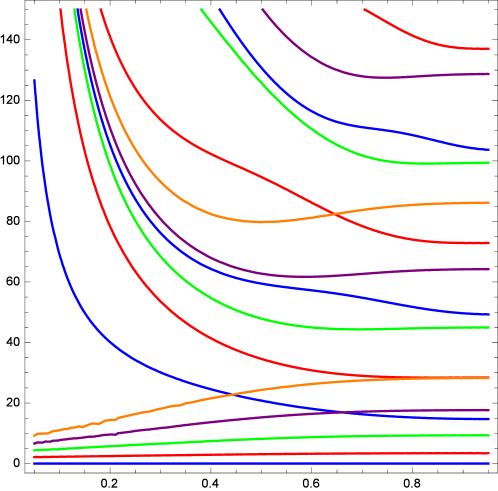
Figure 1. Solution branches of equation (2.6) with $N=2$, $M=\pi$ for $(\varepsilon,\lambda)\in]0,1[\times]0,150[$ . The colors refer to the choice of $l$ in (2.6): blue ($l=0$), red ($l=1$), green ($l=2$), purple ($l=3$), orange ($l=4$).

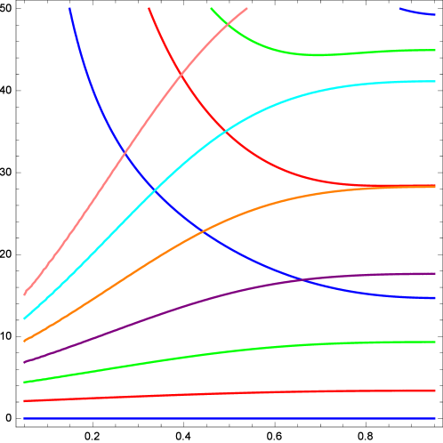
Figure 2. Solution branches of equation (2.6) with $N=2$, $M=\pi$ for $(\varepsilon,\lambda)\in]0,1[\times]0,50[$ . The colors refer to the choice of $l$ in (2.6): blue ($l=0$), red ($l=1$), green ($l=2$), purple ($l=3$), orange ($l=4$), cyan ($l=5$), pink ($l=6$).

It is interesting to compare our results with those in [17], where authors consider the Neumann Laplacian in the annulus $1-\varepsilon<|x|<1$ and prove that for $N=2$ the first positive eigenvalue is a decreasing function of $\varepsilon$. We note that our analysis concerns all eigenvalues $\lambda_{l}$ with arbitrary indexes and multiplicity, and that we do not prove global monotonocity of $\lambda_{l}(\varepsilon)$, which in fact does not hold for any $l$; see Figures 1, 2.

The proof of our results relies on the use of Bessel functions which allows to recast problem (1.4) in the form of an equation $F(\lambda,\varepsilon)=0$ in the unknowns $\lambda,\varepsilon$. Then, after some preparatory work, it is possible to apply the Implicit Function Theorem and conclude. We note that, despite the idea of the proof is rather simple and used also in other contexts (see e.g., [13]), the rigorous application of this method requires lenghty computations, suitable Taylor’s expansions and estimates for the corresponding remainders, as well as recursive formulas for the cross-products of Bessel functions and their derivatives.

Importantly, the multiplicity of the eigenvalues which is often an obstruction in the application of standard asymptotic analysis, does not affect our method.

We note that if the ball $B$ is replaced by a general bounded smooth domain $\Omega$, the convergence of the Neumann eigenvalues to the Steklov eigenvalues when the mass concentrates in a neighborhood of $\partial\Omega$ still holds. However, the explicit computation of the appropriate formula generalizing (1.6) is not easy and requires a completely different technique which will be discussed in a forthcoming paper.

We also note that an asymptotic analysis of similar but different problems is contained in [9, 10], where by the way explicit computations of the coefficients in the asymptotic expansions of the eigenvalues are not provided.

It would be interesting to investigate the monotonicity properties of the Neumann eigenvalues in the case of more general families of mass densities $\rho_{\varepsilon}$. However, we believe that it would be difficult to adapt our method (which is based on explicit representation formulas) even in the case of radial mass densities (note that if $\rho_{\varepsilon}$ is not radial one could obtain a limiting Steklov-type problem with non-constant mass density, see [2] for a general discussion).

This paper is organized as follows. The proof of formula (1.6) is discussed in Section 2. In particular, Subsection 2.1 is devoted to certain technical estimates which are necessary for the rigorous justification of our arguments. In Subsection 2.2 we consider also the case $N=1$ and prove formula (1.6) for $\lambda_{1}$ which, by the way, is the only non zero eigenvalue of the one dimensional Steklov problem. In Appendix we establish the required recursive formulas for the cross-products of Bessel functions and their derivatives which are deduced by the standard formulas available in the literature.

2. Asymptotic behavior of Neumann eigenvalues

It is convenient to use the standard spherical coordinates $(r,\theta)$ in ${\mathbb{R}}^{N}$, where $\theta=(\theta_{1},...\theta_{N-1})$. The corresponding trasformation of coordinates is

$$x_{1} = r\cos(\theta_{1}),$$

$$x_{2} = r\sin(\theta_{1})\cos(\theta_{2}),$$

$$\vdots$$

$$x_{N-1} = r\sin(\theta_{1})\sin(\theta_{2})\cdots\sin(\theta_{N-2})\cos(\theta_{N-1}),$$

$$x_{N} = r\sin(\theta_{1})\sin(\theta_{2})\cdots\sin(\theta_{N-2})\sin(\theta_{N-1}),$$

with $\theta_{1},...,\theta_{N-2}\in[0,\pi]$, $\theta_{N-1}\in[0,2\pi[$ (here it is understood that $\theta_{1}\in[0,2\pi[$ if $N=2$). We denote by $\delta$ the Laplace-Beltrami operator on the unit sphere $\mathbb{S}^{N-1}$ of $\mathbb{R}^{N}$, which can be written in spherical coordinates as

$$\delta=\sum_{j=1}^{N-1}\frac{1}{q_{j}(\sin{\theta_{j}})^{N-j-1}}\frac{\partial}{\partial\theta_{j}}\left((\sin{\theta_{j}})^{N-j-1}\frac{\partial}{\partial\theta_{j}}\right),$$

where

$$q_{1}=1,\ \ \ \ q_{j}=(\sin{\theta_{1}}\sin{\theta_{2}}\cdots\sin_{\theta_{j-1}})^{2},\ \ \ \ j=2,...,N-1,$$

see e.g., [16, p. 40]. To shorten notation, in what follows we will denote by $a$ and $b$ the quantities defined by

$$a=\sqrt{\lambda\varepsilon}(1-\varepsilon),\ \ {\rm and}\ \ b=\sqrt{\lambda\tilde{\rho}_{\varepsilon}}(1-\varepsilon),$$

where

$$\tilde{\rho}_{\varepsilon}=\frac{M-\varepsilon{\omega_{N}}\left(1-\varepsilon\right)^{N}}{\omega_{N}\left(1-\left(1-\varepsilon\right)^{N}\right)}.$$

As customary, we denote by $J_{\nu}$ and $Y_{\nu}$ the Bessel functions of the first and second species and order $\nu$ respectively (recall that $J_{\nu}$ and $Y_{\nu}$ are solutions of the Bessel equation $z^{2}y^{\prime\prime}(z)+zy^{\prime}(z)+(z^{2}-\nu^{2})y(z)=0$).

We begin with the following lemma.

Lemma 2.1.

Given an eigenvalue $\lambda$ of problem (1.4), a corresponding eigenfunction $u$ is of the form $u(r,\theta)=S_{l}(r)H_{l}(\theta)$ where $H_{l}(\theta)$ is a spherical harmonic of some order $l\in\mathbb{N}$ and

(2.2) $$S_{l}(r)=\left\{\begin{array}[]{ll}r^{1-\frac{N}{2}}J_{\nu_{l}}(\sqrt{\lambda\varepsilon}r),&{\rm if\ }r<1-\varepsilon,\\ \\ r^{1-\frac{N}{2}}\left(\alpha J_{\nu_{l}}(\sqrt{\lambda\tilde{\rho}_{\varepsilon}}r)+\beta Y_{\nu_{l}}(\sqrt{\lambda\tilde{\rho}_{\varepsilon}}r)\right),&{\rm if\ }1-\varepsilon<r<1,\end{array}\right.$$

where $\nu_{l}=\frac{(N+2l-2)}{2}$ and $\alpha$, $\beta$ are given by

$${\alpha}={\frac{\pi b}{2}}\left({J_{\nu_{l}}(a)Y_{\nu_{l}}^{\prime}(b)-\frac{a}{b}J_{\nu_{l}}^{\prime}(a)Y_{\nu_{l}}(b)}\right),$$

$${\beta}={\frac{\pi b}{2}}\left({{\frac{a}{b}}J_{\nu_{l}}(b)J_{\nu_{l}}^{\prime}(a)-J_{\nu_{l}}^{\prime}(b)J_{\nu_{l}}(a)}\right).$$

Proof.

Recall that the Laplace operator can be written in spherical coordinates as

$$\Delta=\partial_{rr}+\frac{N-1}{r}\partial_{r}+\frac{1}{r^{2}}\delta.$$

In order to solve the equation $-\Delta u=\lambda\rho_{\varepsilon}u$, we separate variables so that $u(r,\theta)=S(r)H(\theta)$. Then using $l(l+N-2)$, $l\in\mathbb{N}$, as separation constant, we obtain the equations

(2.3) $$r^{2}S^{\prime\prime}+r(N-1)S^{\prime}+r^{2}\lambda\rho_{\varepsilon}S-l(l+N-2)S=0$$

and

(2.4) $$-\delta H=l(l+N-2)H.$$

By setting $S(r)=r^{1-\frac{N}{2}}\tilde{S}(r)$ into (2.3), it follows that $\tilde{S}(r)$ satisfies the Bessel equation

$$\tilde{S}^{\prime\prime}+\frac{1}{r}\tilde{S}^{\prime}+\left(\lambda\rho_{\varepsilon}-\frac{\nu_{l}^{2}}{r^{2}}\right)\tilde{S}=0.$$

Since solutions $u$ of (1.4) are bounded on $\Omega$ and $Y_{\nu_{l}}(z)$ blows up at $z=0$, it follows that for $r<1-\varepsilon$, $S(r)$ is a multiple of the function $r^{1-\frac{N}{2}}J_{\nu_{l}}(\sqrt{\lambda\varepsilon}r)$. For $1-\varepsilon<r<1$, $S(r)$ is a linear combination of the functions $r^{1-\frac{N}{2}}J_{\nu_{l}}(\sqrt{\lambda\tilde{\rho_{\varepsilon}}}r)$ and $r^{1-\frac{N}{2}}Y_{\nu_{l}}(\sqrt{\lambda\tilde{\rho_{\varepsilon}}}r)$. On the other hand, the solutions of (2.4) are the spherical harmonics of order $l$. Then $u$ can be written as in (2.2) for suitable values of $\alpha,\beta\in{\mathbb{R}}$.

Now we compute the coefficients $\alpha$ and $\beta$ in (2.2). Since the right-hand side of the equation in (1.4) is a function in $L^{2}(\Omega)$ then by standard regularity theory a solution $u$ of (1.4) belongs to the standard Sobolev space $H^{2}(\Omega)$, hence $\alpha$ and $\beta$ must be chosen in such a way that $u$ and $\partial_{r}u$ are continuous at $r=1-\varepsilon$, that is

$$\left\{\begin{array}[]{ll}\alpha J_{\nu_{l}}(\sqrt{\lambda\tilde{\rho}_{\varepsilon}}(1-\varepsilon))+\beta Y_{\nu_{l}}(\sqrt{\lambda\tilde{\rho}_{\varepsilon}}(1-\varepsilon))=J_{\nu_{l}}(\sqrt{\lambda\varepsilon}(1-\varepsilon))\,,\\ \alpha J_{\nu_{l}}^{\prime}(\sqrt{\lambda\tilde{\rho}_{\varepsilon}}(1-\varepsilon))+\beta Y_{\nu_{l}}^{\prime}(\sqrt{\lambda\tilde{\rho}_{\varepsilon}}(1-\varepsilon))=\sqrt{\frac{\varepsilon}{\tilde{\rho}_{\varepsilon}}}J_{\nu_{l}}^{\prime}(\sqrt{\lambda\varepsilon}(1-\varepsilon))\,.\end{array}\right.$$

Solving the system we obtain

$$\alpha=\frac{J_{\nu_{l}}(a)Y_{\nu_{l}}^{\prime}(b)-\frac{a}{b}J_{\nu_{l}}^{\prime}(a)Y_{\nu_{l}}(b)}{J_{\nu_{l}}(b)Y_{\nu_{l}}^{\prime}(b)-J_{\nu_{l}}^{\prime}(b)Y_{\nu_{l}}(b)}\ ,\ \ \ \ \beta=\frac{\frac{a}{b}J_{\nu_{l}}(b)J_{\nu_{l}}^{\prime}(a)-J_{\nu_{l}}^{\prime}(b)J_{\nu_{l}}(a)}{J_{\nu_{l}}(b)Y_{\nu_{l}}^{\prime}(b)-J_{\nu_{l}}^{\prime}(b)Y_{\nu_{l}}(b)}.$$

Note that $J_{\nu_{l}}(b)Y_{\nu_{l}}^{\prime}(b)-J_{\nu_{l}}^{\prime}(b)Y_{\nu_{l}}(b)$ is the Wronskian in $b$, which is known to be $\frac{2}{\pi b}$ (see [1, §9]). This concludes the proof. ∎

We are ready to establish an implicit characterization of the eigenvalues of (1.4).

Proposition 2.5.

The nonzero eigenvalues $\lambda$ of problem (1.4) are given implicitly as zeros of the equation

(2.6) $$\left(1-\frac{N}{2}\right)P_{1}(a,b)+\frac{b}{(1-\varepsilon)}P_{2}(a,b)=0$$

where

$$P_{1}(a,b) = J_{\nu_{l}}(a)\left(Y_{\nu_{l}}^{\prime}(b)J_{\nu_{l}}(\frac{b}{1{-}\varepsilon}){-}J_{\nu_{l}}^{\prime}(b)Y_{\nu_{l}}(\frac{b}{1{-}\varepsilon})\right)$$

$${+} \frac{a}{b}J_{\nu_{l}}^{\prime}(a)\left(J_{\nu_{l}}(b)Y_{\nu_{l}}(\frac{b}{1{-}\varepsilon}){-}Y_{\nu_{l}}(b)J_{\nu_{l}}(\frac{b}{1{-}\varepsilon})\right),$$

$$P_{2}(a,b) = J_{\nu_{l}}(a)\left(Y_{\nu_{l}}^{\prime}(b)J_{\nu_{l}}^{\prime}(\frac{b}{1{-}\varepsilon}){-}J_{\nu_{l}}^{\prime}(b)Y_{\nu_{l}}^{\prime}(\frac{b}{1{-}\varepsilon})\right)$$

$${+} \frac{a}{b}J_{\nu_{l}}^{\prime}(a)\left(J_{\nu_{l}}(b)Y_{\nu_{l}}^{\prime}(\frac{b}{1{-}\varepsilon}){-}Y_{\nu_{l}}(b)J_{\nu_{l}}^{\prime}(\frac{b}{1{-}\varepsilon})\right).$$

Proof.

By Lemma 2.1, an eigenfunction $u$ associated with an eigenvalue $\lambda$ is of the form $u(r,\theta)=S_{l}(r)H_{l}(\theta)$ where for $r>1-\varepsilon$

$$S_{l}(r) {=} \frac{\pi b}{2}r^{1{-}\frac{N}{2}}\left[\left(J_{\nu_{l}}(a)Y_{\nu_{l}}^{\prime}(b){-}\frac{a}{b}J_{\nu_{l}}^{\prime}(a)Y_{\nu_{l}}(b)\right)J_{\nu_{l}}(\frac{br}{1-\varepsilon})\right.$$

$${+} \left.\left(\frac{a}{b}J_{\nu_{l}}(b)J_{\nu_{l}}^{\prime}(a){-}J_{\nu_{l}}^{\prime}(b)J_{\nu_{l}}(a)\right)Y_{\nu_{l}}(\frac{br}{1-\varepsilon})\right].$$

We require that $\frac{\partial u}{\partial\nu}=\frac{\partial u}{\partial r}_{|_{r=1}}=0$, which is true if and only if

$$\frac{\pi b}{2}\left(1{-}\frac{N}{2}\right)\left[\left(J_{\nu_{l}}(a)Y_{\nu_{l}}^{\prime}(b){-}\frac{a}{b}J_{\nu_{l}}^{\prime}(a)Y_{\nu_{l}}(b)\right)J_{\nu_{l}}(\frac{b}{1-\varepsilon})\right.\\ {+}\left.\left(\frac{a}{b}J_{\nu_{l}}(b)J_{\nu_{l}}^{\prime}(a){-}J_{\nu_{l}}^{\prime}(b)J_{\nu_{l}}(a)\right)Y_{\nu_{l}}(\frac{b}{1-\varepsilon})\right]\\ {+}\frac{\pi b^{2}}{2(1-\varepsilon)}\left[\left(J_{\nu_{l}}(a)Y_{\nu_{l}}^{\prime}(b){-}\frac{a}{b}J_{\nu_{l}}^{\prime}(a)Y_{\nu_{l}}(b)\right)J_{\nu_{l}}^{\prime}(\frac{b}{1-\varepsilon})\right.\\ {+}\left.\left(\frac{a}{b}J_{\nu_{l}}(b)J_{\nu_{l}}^{\prime}(a){-}J_{\nu_{l}}^{\prime}(b)J_{\nu_{l}}(a)\right)Y_{\nu_{l}}^{\prime}(\frac{b}{1-\varepsilon})\right]=0.$$

The previous equation can be clearly rewritten in the form (2.6). ∎

We now prove the following.

Lemma 2.7.

Equation (2.6) can be written in the form

(2.8) $$\lambda^{2}\varepsilon\left(\frac{M}{3N\omega_{N}}-\frac{1}{\nu_{l}(1+\nu_{l})}\right)+\lambda\varepsilon\left(\frac{N}{2}-\nu_{l}+\frac{(2-N)N\omega_{N}}{2\nu_{l}(1+\nu_{l})M}\right)-2\lambda+\frac{2N\omega_{N}l}{M}$$

$$\qquad\qquad\qquad\qquad\qquad\qquad\quad-\frac{2N\omega_{N}l}{M}\left(\frac{N-1}{2}-\frac{\omega_{N}}{M}-\nu_{l}\right)\varepsilon+\mathcal{R}(\lambda,\varepsilon)=0$$

where $\mathcal{R}(\lambda,\varepsilon)=O(\varepsilon\sqrt{\varepsilon})$ as $\varepsilon\to 0$.

Proof.

We plan to divide the left-hand side of (2.6) by $J_{\nu_{l}}^{\prime}(a)$ and to analyze the resulting terms using the known Taylor’s series for Bessel functions. Note that $J_{\nu_{l}}^{\prime}(a)>0$ for all $\varepsilon$ small enough. We split our analysis into three steps.

Step 1. We consider the term $\frac{P_{2}(a,b)}{J_{\nu_{l}}^{\prime}(a)}$, that is

(2.9) $$\frac{J_{\nu_{l}}(a)}{J_{\nu_{l}}^{\prime}(a)}\left[Y_{\nu_{l}}^{\prime}(b)J_{\nu_{l}}^{\prime}(\frac{b}{1-\varepsilon})-Y_{\nu_{l}}^{\prime}(\frac{b}{1-\varepsilon})J_{\nu_{l}}^{\prime}(b)\right]\\ +\frac{a}{b}\left[Y_{\nu_{l}}^{\prime}(\frac{b}{1-\varepsilon})J_{\nu_{l}}(b)-Y_{\nu_{l}}(b)J_{\nu_{l}}^{\prime}(\frac{b}{1-\varepsilon})\right].$$

Using Taylor’s formula, we write the derivatives of the Bessel functions in (2.9), call them ${\mathcal{C}}^{\prime}_{\nu_{l}}$, as follows

(2.10) $${\mathcal{C}}^{\prime}_{\nu_{l}}\left(\frac{b}{1-\varepsilon}\right)={\mathcal{C}}^{\prime}_{\nu_{l}}(b)+{\mathcal{C}}^{\prime\prime}_{\nu_{l}}(b)\frac{\varepsilon b}{1-\varepsilon}+\dots+\frac{{\mathcal{C}}^{(n)}_{\nu_{l}}(b)}{(n-1)!}\left(\frac{\varepsilon b}{1-\varepsilon}\right)^{n-1}+o\left(\frac{\varepsilon b}{1-\varepsilon}\right)^{n-1}.$$

Then, using (2.10) with $n=4$ for $J_{\nu_{l}}^{\prime}$ and $Y_{\nu_{l}}^{\prime}$ we get

(2.11) $$\frac{J_{\nu_{l}}(a)}{J_{\nu_{l}}^{\prime}(a)}\left[\frac{\varepsilon b}{1-\varepsilon}\left(Y_{\nu_{l}}^{\prime}(b)J_{\nu_{l}}^{\prime\prime}(b)-J_{\nu_{l}}^{\prime}(b)Y_{\nu_{l}}^{\prime\prime}(b)\right)\right.+\frac{\varepsilon^{2}b^{2}}{2(1-\varepsilon)^{2}}\left(Y_{\nu_{l}}^{\prime}(b)J_{\nu_{l}}^{\prime\prime\prime}(b)-J_{\nu_{l}}^{\prime}(b)Y_{\nu_{l}}^{\prime\prime\prime}(b)\right)\\ \left.+\frac{\varepsilon^{3}b^{3}}{6(1-\varepsilon)^{3}}\left(Y_{\nu_{l}}^{\prime}(b)J_{\nu_{l}}^{\prime\prime\prime\prime}(b)-J_{\nu_{l}}^{\prime}(b)Y_{\nu_{l}}^{\prime\prime\prime\prime}(b)\right)+R_{1}(b)\right]\\ +\frac{a}{b}\left[\left(J_{\nu_{l}}(b)Y_{\nu_{l}}^{\prime}(b)-Y_{\nu_{l}}(b)J_{\nu_{l}}^{\prime}(b)\right)+\frac{\varepsilon b}{1-\varepsilon}\left(J_{\nu_{l}}(b)Y_{\nu_{l}}^{\prime\prime}(b)-Y_{\nu_{l}}(b)J_{\nu_{l}}^{\prime\prime}(b)\right)\right.\\ \left.+\frac{\varepsilon^{2}b^{2}}{2(1-\varepsilon)^{2}}\left(J_{\nu_{l}}(b)Y_{\nu_{l}}^{\prime\prime\prime}(b)-Y_{\nu_{l}}(b)J_{\nu_{l}}^{\prime\prime\prime}(b)\right)+R_{2}(b)\right],$$

where

(2.12) $$R_{1}(b)=\sum_{k=4}^{+\infty}\frac{\varepsilon^{k}b^{k}}{k!(1-\varepsilon)^{k}}\biggl{(}Y^{\prime}_{\nu_{l}}(b)J^{(k+1)}_{\nu_{l}}(b)-J^{\prime}_{\nu_{l}}(b)Y_{\nu_{l}}^{(k+1)}(b)\biggr{)}\,$$

and

(2.13) $$R_{2}(b)=\sum_{k=3}^{+\infty}\frac{\varepsilon^{k}b^{k}}{k!(1-\varepsilon)^{k}}\biggl{(}J_{\nu_{l}}(b)Y^{(k+1)}_{\nu_{l}}(b)-Y_{\nu_{l}}(b)J_{\nu_{l}}^{(k+1)}(b)\biggr{)}\,.$$

Let $R_{3}$ be the remainder defined in Lemma 2.25. We set

(2.14) $$R(\lambda,\varepsilon)=R_{3}(a)\left[\frac{\varepsilon b}{1-\varepsilon}\left(Y_{\nu_{l}}^{\prime}(b)J_{\nu_{l}}^{\prime\prime}(b){-}J_{\nu_{l}}^{\prime}(b)Y_{\nu_{l}}^{\prime\prime}(b)\right)\right.\\ {+}\left.\frac{\varepsilon^{2}b^{2}}{2(1-\varepsilon)^{2}}\left(Y_{\nu_{l}}^{\prime}(b)J_{\nu_{l}}^{\prime\prime\prime}(b){-}J_{\nu_{l}}^{\prime}(b)Y_{\nu_{l}}^{\prime\prime\prime}(b)\right)\right.\\ \left.{+}\frac{\varepsilon^{3}b^{3}}{6(1-\varepsilon)^{3}}\left(Y_{\nu_{l}}^{\prime}(b)J_{\nu_{l}}^{\prime\prime\prime\prime}(b){-}J_{\nu_{l}}^{\prime}(b)Y_{\nu_{l}}^{\prime\prime\prime\prime}(b)\right)\right]\\ {+}R_{1}(b)\left[\frac{a}{{\nu_{l}}}{+}\frac{a^{3}}{2{\nu_{l}}^{2}(1+{\nu_{l}})}\right]{+}R_{2}(b)\frac{a}{b}{+}R_{3}(a)R_{1}(b).$$

By Lemma 2.30, it turns out that $R(\lambda,\varepsilon)=O(\varepsilon^{3})$ as $\varepsilon\rightarrow 0$.

We also set

$$f(\varepsilon)=b_{1}^{2}(\varepsilon)a_{1}^{3}(\varepsilon)f_{1}(\varepsilon);$$

$$g(\varepsilon)=b_{1}^{2}(\varepsilon)a_{1}(\varepsilon)g_{1}(\varepsilon)+a_{1}^{3}(\varepsilon)g_{2}(\varepsilon);$$

$$h(\varepsilon)=a_{1}(\varepsilon)h_{1}(\varepsilon)+\varepsilon^{2}\frac{a_{1}^{3}(\varepsilon)}{b_{1}^{2}(\varepsilon)}h_{2}(\varepsilon);$$

$$k(\varepsilon)=\frac{a_{1}(\varepsilon)}{b_{1}^{2}(\varepsilon)}k_{1}(\varepsilon),$$

where

$$a_{1}(\varepsilon)=\frac{a}{\sqrt{\lambda\varepsilon}}=(1-\varepsilon);$$

$$b_{1}(\varepsilon)=b\sqrt{\frac{\varepsilon}{\lambda}};$$

$$f_{1}(\varepsilon)=\frac{1}{6{\nu_{l}}^{2}(1+{\nu_{l}})(1-\varepsilon)^{3}};$$

$$g_{1}(\varepsilon)=\frac{1}{3{\nu_{l}}(1-\varepsilon)^{3}};$$

$$g_{2}(\varepsilon)=-\frac{1}{{\nu_{l}}^{2}(1+{\nu_{l}})(1-\varepsilon)}+\frac{\varepsilon}{2{\nu_{l}}^{2}(1+{\nu_{l}})(1-\varepsilon)^{2}}-\frac{\varepsilon^{2}(3+2{\nu_{l}}^{2})}{6{\nu_{l}}^{2}(1+{\nu_{l}})(1-\varepsilon)^{3}};$$

$$h_{1}(\varepsilon)=-\frac{2}{{\nu_{l}}(1-\varepsilon)}+\frac{\varepsilon}{{\nu_{l}}(1-\varepsilon)^{2}}-\frac{\varepsilon^{2}(3+2{\nu_{l}}^{2})}{3{\nu_{l}}(1-\varepsilon)^{3}}-\frac{\varepsilon}{(1-\varepsilon)^{2}};$$

$$h_{2}(\varepsilon)=\frac{1}{(1+{\nu_{l}})(1-\varepsilon)}-\frac{3\varepsilon}{2(1+{\nu_{l}})(1-\varepsilon)^{2}}+\frac{\varepsilon^{2}({\nu_{l}}^{4}+11{\nu_{l}}^{2})}{6{\nu_{l}}^{2}(1+{\nu_{l}})(1-\varepsilon)^{3}};$$

$$k_{1}(\varepsilon)=2+\frac{2\varepsilon{\nu_{l}}}{(1-\varepsilon)}-\frac{3\varepsilon^{2}{\nu_{l}}}{(1-\varepsilon)^{2}}+\frac{\varepsilon^{3}({\nu_{l}}^{4}+11{\nu_{l}}^{2})}{3\nu_{l}(1-\varepsilon)^{3}}-\frac{2\varepsilon}{(1-\varepsilon)}+\frac{\varepsilon^{2}(2+{\nu_{l}}^{2})}{(1-\varepsilon)^{2}}.$$

Note that functions $f,g,h,k$ are continuous at $\varepsilon=0$ and $f(0),g(0),h(0),k(0)\neq 0$.

Using the explicit formulas for the cross products of Bessel functions given by Lemma 3.2 and Corollary 3.7 in (2.11), (2.9) can be written as

(2.15) $$\frac{1}{\sqrt{\lambda}\pi}\varepsilon\sqrt{\varepsilon}k(\varepsilon)+\frac{\sqrt{\lambda}}{\pi}\varepsilon\sqrt{\varepsilon}h(\varepsilon)+\frac{\lambda\sqrt{\lambda}}{\pi}\varepsilon^{2}\sqrt{\varepsilon}g(\varepsilon)+\frac{\lambda^{2}\sqrt{\lambda}}{\pi}\varepsilon^{3}\sqrt{\varepsilon}f(\varepsilon)+R(\lambda,\varepsilon).$$

Step 2. We consider the quantity $\frac{P_{1}(a,b)}{J_{\nu_{l}}^{\prime}(a)}$, that is

(2.16) $$\frac{J_{\nu_{l}}(a)}{J_{\nu_{l}}^{\prime}(a)}\left[Y_{\nu_{l}}^{\prime}(b)J_{\nu_{l}}(\frac{b}{1-\varepsilon})-J_{\nu_{l}}^{\prime}(b)Y_{\nu_{l}}(\frac{b}{1-\varepsilon})\right]\\ +\frac{a}{b}\left[J_{\nu_{l}}(b)Y_{\nu_{l}}(\frac{b}{1-\varepsilon})-Y_{\nu_{l}}(b)J_{\nu_{l}}(\frac{b}{1-\varepsilon})\right].$$

Proceeding as in Step 1 and setting

$$\tilde{f}(\varepsilon)=-\frac{a_{1}^{3}(\varepsilon)b_{1}(\varepsilon)}{2\pi{\nu_{l}}^{2}(1+{\nu_{l}})(1-\varepsilon)^{2}};$$

$$\tilde{g}(\varepsilon)=\frac{a_{1}^{3}(\varepsilon)}{b_{1}(\varepsilon)}\left(\frac{1}{\pi{\nu_{l}}^{2}(1+{\nu_{l}})}+\frac{\varepsilon^{2}}{2\pi(1+{\nu_{l}})(1-\varepsilon)^{2}}\right)-\frac{a_{1}(\varepsilon)b_{1}(\varepsilon)}{{\nu_{l}}\pi(1-\varepsilon)^{2}};$$

$$\tilde{h}(\varepsilon)=\frac{a_{1}(\varepsilon)}{b_{1}(\varepsilon)}\left(\frac{2}{{\nu_{l}}\pi}+\frac{2\varepsilon}{\pi(1-\varepsilon)}+\frac{({\nu_{l}}-1)}{\pi(1-\varepsilon)^{2}}\varepsilon^{2}\right),$$

one can prove that (2.16) can be written as

(2.17) $$\varepsilon\tilde{h}(\varepsilon)+\lambda\varepsilon^{2}\tilde{g}(\varepsilon)+\lambda^{2}\varepsilon^{3}\tilde{f}(\varepsilon)+\hat{R}(\lambda,\varepsilon),$$

where $\hat{R}({\lambda,\varepsilon})=O(\varepsilon^{2}\sqrt{\varepsilon})$ as $\varepsilon\rightarrow 0$; see Lemma 2.30.

Step 3. We combine (2.15) and (2.17) and rewrite equation (2.6) in the form

(2.18) $$\varepsilon(1-\frac{N}{2})\tilde{h}(\varepsilon)+\varepsilon\frac{b_{1}(\varepsilon)k(\varepsilon)}{\pi(1-\varepsilon)}+\lambda\varepsilon^{2}(1-\frac{N}{2})\tilde{g}(\varepsilon)+\lambda\varepsilon\frac{b_{1}(\varepsilon)h(\varepsilon)}{\pi(1-\varepsilon)}\\ +\lambda^{2}\varepsilon^{3}(1-\frac{N}{2})\tilde{f}(\varepsilon)+\lambda^{2}\varepsilon^{2}\frac{b_{1}(\varepsilon)g(\varepsilon)}{\pi(1-\varepsilon)}+\lambda^{3}\varepsilon^{3}\frac{b_{1}(\varepsilon)f(\varepsilon)}{\pi(1-\varepsilon)}+\mathcal{R}_{0}(\lambda,\varepsilon)=0,$$

where

$$\mathcal{R}_{0}(\lambda,\varepsilon)=\frac{\sqrt{\lambda}b_{1}(\varepsilon)}{(1-\varepsilon)\sqrt{\varepsilon}}R(\lambda,\varepsilon)+\left(1-\frac{N}{2}\right)\hat{R}(\lambda,\varepsilon).$$

Note that $\mathcal{R}_{0}(\lambda,\varepsilon)=O(\varepsilon^{2}\sqrt{\varepsilon})$ as $\varepsilon\rightarrow 0$. Dividing by $\varepsilon$ in (2.18) and setting $\mathcal{R}_{1}(\lambda,\varepsilon)=\frac{\mathcal{R}_{0}(\lambda,\varepsilon)}{\varepsilon}$, we obtain

(2.19) $$(1-\frac{N}{2})\tilde{h}(\varepsilon)+\frac{b_{1}(\varepsilon)k(\varepsilon)}{\pi(1-\varepsilon)}+\lambda\varepsilon(1-\frac{N}{2})\tilde{g}(\varepsilon)+\lambda\frac{b_{1}(\varepsilon)h(\varepsilon)}{\pi(1-\varepsilon)}$$

$$+\lambda^{2}\varepsilon^{2}(1-\frac{N}{2})\tilde{f}(\varepsilon)+\lambda^{2}\varepsilon\frac{b_{1}(\varepsilon)g(\varepsilon)}{\pi(1-\varepsilon)}+\lambda^{3}\varepsilon^{2}\frac{b_{1}(\varepsilon)f(\varepsilon)}{\pi(1-\varepsilon)}+\mathcal{R}_{1}(\lambda,\varepsilon)=0.$$

We now multiply in (2.19) by $\frac{\pi\nu_{l}(1-\varepsilon)}{b_{1}(\varepsilon)}$ which is a positive quantity for all $0<\varepsilon<1$. Taking into account the definitions of functions $g,h,k,\tilde{g},\tilde{h}$, we can finally rewrite (2.19) in the form

(2.20) $$\lambda^{2}\varepsilon\left(\frac{\hat{\rho}(\varepsilon)}{3}-\frac{1}{\nu_{l}(1+\nu_{l})}\right)+\lambda\varepsilon\left(\frac{N}{2}-\nu_{l}+\frac{2-N}{2\nu_{l}(1+\nu_{l})\hat{\rho}(\varepsilon)}\right)-2\lambda$$

$$\qquad\qquad\qquad\qquad\qquad\qquad\qquad\qquad\qquad\qquad+\frac{2l\left(1+\varepsilon\nu_{l}\right)}{\hat{\rho}(\varepsilon)}+\mathcal{R}(\lambda,\varepsilon)=0,$$

where

$$\hat{\rho}(\varepsilon)=\varepsilon\tilde{\rho}(\varepsilon)=\frac{M-\omega_{N}\varepsilon(1-\varepsilon)^{N}}{\omega_{N}\left(N-\frac{N(N-1)}{2}\varepsilon-\sum_{k=3}^{N}\binom{N}{k}(-1)^{k}\varepsilon^{k-1}\right)},$$

and $\mathcal{R}(\lambda,\varepsilon)=O(\varepsilon\sqrt{\varepsilon})$ as $\varepsilon\to 0$. The formulation in (2.8) can be easily deduced by observing that

$$\hat{\rho}_{\varepsilon}=\frac{M}{N\omega_{N}}+2\frac{M}{N\omega_{N}}\left(\frac{N-1}{4}-\frac{\omega_{N}}{2M}\right)\varepsilon+O(\varepsilon^{2}),\ \ {\rm as}\ \varepsilon\to 0.$$

∎

We are now ready to prove our main result

Theorem 2.21.

All eigenvalues of problem (1.4) have the following asymptotic behavior

(2.22) $$\lambda_{l}(\varepsilon)=\lambda_{l}+\left(\frac{2l\lambda_{l}}{3}+\frac{2\lambda^{2}_{l}}{N(2l+N)}\right)\varepsilon+o(\varepsilon),\ \ \ {\rm as}\ \varepsilon\to 0,$$

where $\lambda_{l}$ are the eigenvalues of problem (1.1).

Moreover, for each $l\in{\mathbb{N}}$ the function defined by $\lambda_{l}(\varepsilon)$ for $\varepsilon>0$ and $\lambda_{l}(0)=\lambda_{l}$, is continuous in the whole of $[0,1[$ and of class $C^{1}$ in a neighborhood of $\varepsilon=0$.

Proof.

By using the Min-Max Principle and related standard arguments, one can easily prove that $\lambda_{l}(\varepsilon)$ depends with continuity on $\varepsilon>0$ (cfr. [15], see also [12]). Moreover, by using (1.5) the maps $\varepsilon\mapsto\lambda_{l}(\varepsilon)$ can be extended by continuity at the point $\varepsilon=0$ by setting $\lambda_{l}(0)=\lambda_{l}$.

In order to prove differentiability of $\lambda_{l}(\varepsilon)$ around zero and the validity of (2.22), we consider equation (2.8) and apply the Implicit Function Theorem. Note that equation (2.8) can be written in the form $F(\lambda,\varepsilon)=0$ where $F$ is a function of class $C^{1}$ in the variables $(\lambda,\varepsilon)\in]0,\infty[\times[0,1[$, with

$$F(\lambda,0) = -2\lambda+\frac{2N\omega_{N}l}{M},$$

$$F^{\prime}_{\lambda}(\lambda,0) = -2,$$

(2.23) $$F^{\prime}_{\varepsilon}(\lambda,0) = \lambda^{2}\left(\frac{M}{3N\omega_{N}}-\frac{1}{\nu_{l}(1+\nu_{l})}\right)+\lambda\left(\frac{N}{2}-\nu_{l}+\frac{(2-N)N\omega_{N}}{2\nu_{l}(1+\nu_{l})M}\right)$$

$$-\frac{2N\omega_{N}l}{M}\left(\frac{N-1}{2}-\frac{\omega_{N}}{M}-\nu_{l}\right)$$

By (1.2), $\lambda_{l}=N\omega_{N}l/M$ hence $F(\lambda_{l},0)=0$. Since $F^{\prime}_{\lambda}(\lambda_{l},0)\neq 0$, the Implicit Function Theorem combined with the continuity of the functions $\lambda_{l}(\cdot)$ allows to conclude that functions $\lambda_{l}(\cdot)$ are of class $C^{1}$ around zero.

We now compute the derivative of $\lambda_{l}(\cdot)$ at zero. Using the equality $N\omega_{N}/M=\lambda_{l}/l$ and recalling that $\nu_{l}=l+N/2-1$ we get

$$F^{\prime}_{\varepsilon}(\lambda_{l},0) = \lambda_{l}^{2}\left(\frac{l}{3\lambda_{l}}-\frac{1}{\nu_{l}(1+\nu_{l})}\right)+\lambda_{l}\left(1-l+\frac{\lambda_{l}(2-N)}{2l\nu_{l}(1+\nu_{l})}\right)-2\lambda_{l}\left(\frac{1}{2}-l-\frac{\lambda_{l}}{Nl}\right)$$

$$= \lambda_{l}^{2}\left(\frac{1}{\nu_{l}(1+\nu_{l})}\left(\frac{2-N}{2l}-1\right)+\frac{2}{Nl}\right)+\frac{4}{3}\lambda_{l}l=\frac{4\lambda^{2}_{l}}{N^{2}+2Nl}+\frac{4}{3}\lambda_{l}l.$$

Finally, formula $\lambda^{\prime}_{l}(0)=-F^{\prime}_{\varepsilon}(\lambda_{l},0)/F^{\prime}_{\lambda}(\lambda_{l},0)$ yields (1.6) and the validity of (2.22). ∎

Corollary 2.24.

For any $l\in{\mathbb{N}}\setminus\{0\}$ there exists $\delta_{l}$ such that the function $\lambda_{l}(\cdot)$ is strictly increasing in the interval $[0,\delta_{l}[$. In particular, $\lambda_{l}<\lambda_{l}(\varepsilon)$ for all $\varepsilon\in]0,\delta_{l}[$.

2.1. Estimates for the remainders

This subsection is devoted to the proof of a few technical estimates used in the proof of Lemma 2.7.

Lemma 2.25.

The function $R_{3}$ defined by

(2.26) $$\frac{J_{\nu}(z)}{J_{\nu}^{\prime}(z)}=\frac{z}{{\nu}}+\frac{z^{3}}{2{\nu}^{2}(1+{\nu})}+R_{3}(z),$$

is $O(z^{5})$ as $z\rightarrow 0$.

Proof.

Recall the well-known following representation of the Bessel functions of the first species

(2.27) $$J_{\nu}(z)=\left(\frac{z}{2}\right)^{\nu}\sum_{j=0}^{+\infty}\frac{(-1)^{j}}{j!\Gamma(j+{\nu}+1)}\left(\frac{z}{2}\right)^{2j}.$$

For clarity, we simply write

(2.28) $$J_{\nu}(z)=z^{\nu}(a_{0}+a_{2}z^{2}+a_{4}z^{4}+O(z^{5})),$$

hence

(2.29) $$J_{\nu}^{\prime}(z)=z^{\nu-1}(\nu a_{0}+(\nu+2)a_{2}z^{2}+(\nu+4)a_{4}z^{4}+O(z^{5}))$$

where the coefficients $a_{0},a_{2},a_{4}$ are defined by (2.27). By (2.28), (2.29) and standard computations it follows that

$$\frac{J_{\nu}(z)}{J_{\nu}^{\prime}(z)}=\frac{z}{\nu}-{\frac{2a_{2}}{\nu^{2}a_{0}}}z^{3}+O(z^{5}),$$

which gives exactly (2.26). ∎

Lemma 2.30.

For any $\lambda>0$ the remainders $R(\lambda,\varepsilon)$ and $\hat{R}(\lambda,\varepsilon)$ defined in the proof of Lemma 2.7 are $O(\varepsilon^{3})$, $O(\varepsilon^{2}\sqrt{\varepsilon})$, respectively, as $\varepsilon\rightarrow 0$. Moreover, the same holds true for the corresponding partial derivatives $\partial_{\lambda}R(\lambda,\varepsilon)$, $\partial_{\lambda}\hat{R}(\lambda,\varepsilon)$.

Proof.

First, we consider $R_{3}(a)=R_{3}(\sqrt{\lambda\varepsilon}(1-\varepsilon))$ where $R_{3}$ is defined in Lemma 2.25 and we differentiate it with respect to $\lambda$. We obtain

$$\frac{\partial R_{3}(a)}{\partial\lambda}=\frac{aR_{3}^{\prime}(a)}{2\lambda},$$

hence by Lemma 2.25 we can conclude that $R_{3}(a)$ and $\frac{\partial R_{3}(a)}{\partial\lambda}$ are $O(\varepsilon^{2}\sqrt{\varepsilon})$ as $\varepsilon\rightarrow 0$.

Now consider $R_{1}(b)$ and $R_{2}(b)$ defined in (2.12), (2.13). Since $\lambda>0$, we have that $b>0$ hence the Bessel functions are analytic in $b$ and we can write

$$2\sqrt{\lambda}\frac{\partial R_{1}(b)}{\partial\lambda} = \frac{\varepsilon b_{1}(\varepsilon)}{\sqrt{\varepsilon}(1-\varepsilon)}\sum_{k=4}^{+\infty}\frac{b^{k-1}\varepsilon^{k-1}}{(k-1)!(1-\varepsilon)^{k-1}}\left(Y_{\nu}^{\prime}(b)J_{\nu}^{(k+1)}(b)-J_{\nu}^{\prime}(b)Y_{\nu}^{(k+1)}(b)\right)$$

$$+ \frac{b_{1}(\varepsilon)}{\sqrt{\varepsilon}}\sum_{k=4}^{+\infty}\frac{\varepsilon^{k}b^{k}}{k!(1-\varepsilon)^{k}}\left(Y_{\nu}^{\prime}(b)J_{\nu}^{(k+1)}(b)-J_{\nu}^{\prime}(b)Y_{\nu}^{(k+1)}(b)\right)^{\prime}.$$

Here and in the sequel we write $\nu$ instead of $\nu_{l}$. Using the fact that $b=\sqrt{\lambda/\varepsilon}b_{1}(\varepsilon)$ and Lemma 3.2 we conclude that all the cross products of the form $Y_{\nu}^{\prime}(b)J_{\nu}^{(k+1)}(b)-J_{\nu}^{\prime}(b)Y_{\nu}^{(k+1)}(b)$ and their derivatives $(Y_{\nu}^{\prime}(b)J_{\nu}^{(k+1)}(b)-J_{\nu}^{\prime}(b)Y_{\nu}^{(k+1)}(b))^{\prime}$ are $O(\sqrt{\varepsilon})$ and $O(\varepsilon)$ respectively, as $\varepsilon\rightarrow 0$. It follows that $R_{1}(b)$ and $\partial_{\lambda}R_{1}(b)$ are $O(\varepsilon^{2}\sqrt{\varepsilon})$ as $\varepsilon\rightarrow 0$.

Similarly,

$$2\sqrt{\lambda}\frac{\partial R_{2}(b)}{\partial\lambda} = \frac{\varepsilon b_{1}(\varepsilon)}{\sqrt{\varepsilon}(1-\varepsilon)}\sum_{k=3}^{+\infty}\frac{b^{k-1}\varepsilon^{k-1}}{(k-1)!(1-\varepsilon)^{k-1}}\left(J_{\nu}(b)Y_{\nu}^{(k+1)}(b)-Y_{\nu}(b)J_{\nu}^{(k+1)}(b)\right)$$

$$+ \frac{b_{1}(\varepsilon)}{\sqrt{\varepsilon}}\sum_{k=3}^{+\infty}\frac{\varepsilon^{k}b^{k}}{k!(1-\varepsilon)^{k}}\left(J_{\nu}(b)Y_{\nu}^{(k+1)}(b)-Y_{\nu}(b)J_{\nu}^{(k+1)}(b)\right)^{\prime},$$

hence $R_{2}(b)$ and $\partial_{\lambda}R_{2}(b)$ are $O(\varepsilon^{2})$ as $\varepsilon\rightarrow 0$.

Summing up all the terms, using Lemma 3.1 and Corollary 3.7, we obtain

$$R(\lambda,\varepsilon)=R_{3}(a)\left[\frac{2\varepsilon}{\pi(1-\varepsilon)}\left(\frac{{\nu}^{2}}{b^{2}}-1\right){+}\frac{\varepsilon^{2}}{\pi(1-\varepsilon)^{2}}\left(1-\frac{3{\nu}^{2}}{b^{2}}\right)\right.\\ \left.{+}\frac{\varepsilon^{3}b^{2}}{3\pi(1-\varepsilon)^{3}}\left(\frac{{\nu}^{4}+11{\nu}^{2}}{b^{4}}-\frac{3+2{\nu}^{2}}{b^{2}}+1\right)\right]\\ +R_{1}(b)\left[\frac{a}{{\nu}}+\frac{a^{3}}{2{\nu}^{2}(1+{\nu})}\right]{+}R_{2}(b)\frac{a}{b}{+}R_{3}(a)R_{1}(b).$$

We conclude that $R(\lambda,\varepsilon)$ is $O(\varepsilon^{3})$ as $\varepsilon\rightarrow 0$. Moreover, it easily follows that $\frac{\partial R(\lambda,\varepsilon)}{\partial\lambda}$ is also $O(\varepsilon^{3})$ as $\varepsilon\rightarrow 0$.

The proof of the estimates for $\hat{R}$ and its derivatives is similar and we omit it. ∎

Remark 2.31.

According to standard Landau’s notation, saying that a function $f(z)$ is $O(g(z))$ as $z\to 0$ means that there exists $C>0$ such that $|f(z)|\leq C|g(z)|$ for any $z$ sufficiently close to zero. Thus, using Landau’s notation in the statements of Lemmas 2.7, 2.30 understands the existence of such constants $C$, which in principle may depend on $\lambda>0$. However, a careful analysis of the proofs reveals that given a bounded interval of the type $[A,B]$ with $0<A<B$ then the appropriate constants $C$ in the estimates can be taken independent of $\lambda\in[A,B]$.

2.2. The case $N=1$

We include here a description of the case $N=1$ for the sake of completeness. Let $\Omega$ be the open interval $]-1,1[$. Problem (1.1) reads

(2.32) $$\begin{cases}u^{\prime\prime}(x)=0,&{\rm for}\ x\in]-1,1[,\\ u^{\prime}(\pm 1)=\pm\lambda\frac{M}{2}u(\pm 1),\end{cases}$$

in the unknowns $\lambda$ and $u$. It is easy to see that the only eigenvalues are $\lambda_{0}=0$ and $\lambda_{1}=\frac{2}{M}$ and they are associated with the constant functions and the function $x$, respectively. As in (1.3), we define a mass density $\rho_{\varepsilon}$ on the whole of $]-1,1[$ by

$$\rho_{\varepsilon}(x)=\left\{\begin{array}[]{ll}\frac{M}{2\varepsilon}-1+\varepsilon&{\rm if\ }x\in]-1,-1+\varepsilon[\cup]1-\varepsilon,1[,\\ \varepsilon&{\rm if\ }x\in]-1+\varepsilon,1-\varepsilon[.\end{array}\right.$$

Note that for any $x\in]-1,1[$ we have $\rho_{\varepsilon}(x)\to 0$ as $\varepsilon\to 0$, and $\int_{-1}^{1}\rho_{\varepsilon}dx=M$ for all $\varepsilon>0$. Problem (1.4) for $N=1$ reads

(2.33) $$\left\{\begin{array}[]{ll}-u^{\prime\prime}(x)=\lambda\rho_{\varepsilon}(x)u(x),&{\rm for}\ x\in]-1,1[,\\ u^{\prime}(-1)=u^{\prime}(1)=0.\end{array}\right.$$

It is well-known from Sturm-Liouville theory that problem (2.33) has an increasing sequence of non-negative eigenvalues of multiplicity one. We denote the eigenvalues of (2.33) by $\lambda_{l}(\varepsilon)$ with $l\in\mathbb{N}$. For any $\varepsilon\in]0,1[$, the only zero eigenvalue is $\lambda_{0}(\varepsilon)$ and the corresponding eigenfunctions are the constant functions.

We establish an implicit characterization of the eigenvalues of (2.33).

Proposition 2.34.

The nonzero eigenvalues $\lambda$ of problem (2.33) are given implicitly as zeros of the equation

(2.35) $$2\sqrt{\varepsilon\left(\frac{M}{2\varepsilon}-1+\varepsilon\right)}\cos{(2\sqrt{\lambda\varepsilon}(1-\varepsilon))}\sin{\left(2\varepsilon\sqrt{\lambda\left(\frac{M}{2\varepsilon}-1+\varepsilon\right)}\right)}\\ +\left[-\frac{M}{2\varepsilon}+1+\left(\frac{M}{2\varepsilon}-1+2\varepsilon\right)\cos{\left(2\varepsilon\sqrt{\lambda\left(\frac{M}{2\varepsilon}-1+\varepsilon\right)}\right)}\right]\sin{\left(2\sqrt{\lambda\varepsilon}(1-\varepsilon)\right)}=0.$$

Proof.

Given an eigenvalue $\lambda>0$, a solution of (2.33) is of the form

$$u(x)=\left\{\begin{array}[]{ll}A\cos{(\sqrt{\lambda\rho_{2}}x)}+B\sin{(\sqrt{\lambda\rho_{2}}x)},&{\rm for\ }x\in]-1,-1+\varepsilon[,\\ \\ C\cos{(\sqrt{\lambda\rho_{1}}x)}+D\sin{(\sqrt{\lambda\rho_{1}}x)},&{\rm for\ }x\in]-1+\varepsilon,1-\varepsilon[,\\ \\ E\cos{(\sqrt{\lambda\rho_{2}}x)}+F\sin{(\sqrt{\lambda\rho_{2}}x)},&{\rm for\ }x\in]1-\varepsilon,1[,\end{array}\right.$$

where $\rho_{1}=\varepsilon,\rho_{2}=\frac{M}{2\varepsilon}-1+\varepsilon$ and $A,B,C,D,E,F$ are suitable real numbers. We impose the continuity of $u$ and $u^{\prime}$ at the points $x=-1+\varepsilon$ and $x=1-\varepsilon$ and the boundary conditions, obtaining a homogeneous system of six linear equations in six unknowns of the form $\mathcal{M}v=0$, where $v=(A,B,C,D,E,F)$ and $\mathcal{M}$ is the matrix associated with the system. We impose the condition ${\rm det}\mathcal{M}=0$. This yields formula (2.35). ∎

Note that $\lambda=0$ is a solution for all $\varepsilon>0$, then we consider only the case of nonzero eigenvalues. Using standard Taylor’s formulas, we easily prove the following

Lemma 2.36.

Equation (2.35) can be rewritten in the form

(2.37) $$M-\frac{\lambda M^{2}}{2}+\frac{\lambda M^{2}}{6}\left(1+\lambda\left(2+\frac{M}{2}\right)\right)\varepsilon+R(\lambda,\varepsilon)=0,$$

where $R(\lambda,\varepsilon)=O(\varepsilon^{2})$ as $\varepsilon\rightarrow 0$.

Finally, we can prove the following theorem. Note that formula (2.39) is the same as (2.22) with $N=1,l=1$.

Theorem 2.38.

The first eigenvalue of problem (2.33) has the following asymptotic behavior

(2.39) $$\lambda_{1}(\varepsilon)=\lambda_{1}+\frac{2}{3}(\lambda_{1}+\lambda_{1}^{2})\varepsilon+o(\varepsilon)\ \ \ {\rm as}\ \varepsilon\to 0,$$

where $\lambda_{1}=2/M$ is the only nonzero eigenvalue of problem (2.32). Moreover, for $l>1$ we have that $\lambda_{l}(\varepsilon)\rightarrow+\infty$ as $\varepsilon\rightarrow 0$.

Proof.

The proof is similar to that of Theorem 2.21. It is possible to prove that the eigenvalues $\lambda_{l}(\varepsilon)$ of (2.33) depend with continuity on $\varepsilon>0$. We consider equation (2.37) and apply the Implicit Function Theorem. Equation (2.37) can be written in the form $F(\lambda,\varepsilon)=0$, with $F$ of class $C^{1}$ in $]0,+\infty[\times[0,1[$ with $F(\lambda,0)=M-\frac{\lambda M^{2}}{2}$, $F_{\lambda}^{\prime}(\lambda,0)=-\frac{M^{2}}{2}$ and $F_{\varepsilon}^{\prime}(\lambda,0)=\frac{\lambda M^{2}}{6}(1+\lambda(2+\frac{M}{2}))$.

Since $\lambda_{1}=\frac{2}{M}$, $F(\lambda_{1},0)=0$ and $F_{\lambda}^{\prime}(\lambda_{1},0)\neq 0$, the zeros of equation (2.39) in a neighborhood of $(\lambda,0)$ are given by the graph of a $C^{1}$-function $\varepsilon\mapsto\lambda(\varepsilon)$ with $\lambda(0)=\lambda_{1}$. We note that $\lambda(\varepsilon)=\lambda_{1}(\varepsilon)$ for all $\varepsilon$ small enough. Indeed, assuming by contradiction that $\lambda(\varepsilon)=\lambda_{l}(\varepsilon)$ with $l\geq 2$, we would obtain that, possibly passing to a subsequence, $\lambda_{1}(\varepsilon)\to\bar{\lambda}$ as $\varepsilon\to 0$, for some $\bar{\lambda}\in[0,\lambda_{1}[$. Then passing to the limit in (2.37) as $\varepsilon\to 0$ we would obtain a contradiction. Thus, $\lambda_{1}(\cdot)$ is of class $C^{1}$ in a neighborhood of zero and $\lambda_{1}^{\prime}(0)=-F^{\prime}_{\varepsilon}(\lambda_{1},0)/F^{\prime}_{\lambda}(\lambda_{1},0)$ which yields formula (2.39).

The divergence as $\varepsilon\to 0$ of the higher eigenvalues $\lambda_{l}(\varepsilon)$ with $l>1$, is clearly deduced by the fact that the existence of a converging subsequence of the form $\lambda_{l}(\varepsilon_{n})$, $n\in{\mathbb{N}}$ would provide the existence of an eigenvalue for the limiting problem (2.32) different from $\lambda_{0}$ and $\lambda_{1}$, which is not admissible.

∎

3. Appendix

We provide here explicit formulas for the cross products of Bessel functions used in this paper.

Lemma 3.1.

The following identities hold

$$Y_{\nu}(z)J_{\nu}^{\prime}(z)-J_{\nu}(z)Y_{\nu}^{\prime}(z) = -\frac{2}{\pi z},$$

$$Y_{\nu}(z)J_{\nu}^{\prime\prime}(z)-J_{\nu}(z)Y_{\nu}^{\prime\prime}(z) = \frac{2}{\pi z^{2}},$$

$$Y_{\nu}^{\prime}(z)J_{\nu}^{\prime\prime}(z)-J_{\nu}^{\prime}(z)Y_{\nu}^{\prime\prime}(z) = \frac{2}{\pi z}\left(\frac{{\nu}^{2}}{z^{2}}-1\right),$$

Proof.

It is well-known (see [1, §9]) that

$$J_{\nu}(z)Y_{\nu}^{\prime}(z)-Y_{\nu}(z)J_{\nu}^{\prime}(z)=J_{{\nu}+1}(z)Y_{\nu}(z)-J_{\nu}(z)Y_{{\nu}+1}(z)=\frac{2}{\pi z},$$

which gives the first identity in the statement. The second identity holds since

$$J_{\nu}(z)Y_{\nu}^{\prime\prime}(z)-Y_{\nu}(z)J_{\nu}^{\prime\prime}(z) = \left(J_{\nu}(z)Y_{\nu}^{\prime}(z)-Y_{\nu}(z)J_{\nu}^{\prime}(z)\right)^{\prime}=\left(\frac{2}{\pi z}\right)^{\prime}=-\frac{2}{\pi z^{2}}.$$

The third identity holds since

$$Y_{\nu}^{\prime}(z)J_{\nu}^{\prime\prime}(z)-J_{\nu}^{\prime}(z)Y_{\nu}^{\prime\prime}(z)=Y_{\nu}^{\prime}(z)\left(J_{{\nu}-1}(z)-\frac{{\nu}}{z}J_{\nu}(z)\right)^{\prime}-J_{\nu}^{\prime}(z)\left(Y_{{\nu}-1}(z)-\frac{{\nu}}{z}Y_{\nu}(z)\right)^{\prime}\\ =Y_{\nu}^{\prime}(z)J_{{\nu}-1}^{\prime}(z)-J_{\nu}^{\prime}(z)Y_{{\nu}-1}^{\prime}(z)+\frac{{\nu}}{z^{2}}\left(Y_{\nu}^{\prime}(z)J_{\nu}(z)-J_{\nu}^{\prime}(z)Y_{\nu}(z)\right)\\ =\left(Y_{\nu}^{\prime}(z)\frac{1}{2}\left(J_{{\nu}-2}(z)-J_{\nu}(z)\right)-J_{\nu}^{\prime}(z)\frac{1}{2}\left(Y_{{\nu}-2}(z)-Y_{\nu}(z)\right)\right)+\frac{2{\nu}}{\pi z^{3}}\\ =\frac{1}{2}\left(Y_{\nu}^{\prime}(z)J_{{\nu}-2}(z)-J_{\nu}^{\prime}(z)Y_{{\nu}-2}(z)\right)\\ -\frac{1}{2}\left(Y_{\nu}^{\prime}(z)J_{\nu}(z)-J_{\nu}^{\prime}(z)Y_{\nu}(z)\right)+\frac{2{\nu}}{\pi z^{3}}\\ =\frac{1}{2}\left(J_{\nu}^{\prime}(z)Y_{\nu}(z)-Y_{\nu}^{\prime}(z)J_{\nu}(z)\right)\\ +\frac{{\nu}-1}{z}\left(Y_{\nu}^{\prime}(z)J_{{\nu}-1}(z)-J_{\nu}^{\prime}(z)Y_{{\nu}-1}(z)\right)-\frac{1}{\pi z}+\frac{2{\nu}}{\pi z^{3}}\\ =\frac{{\nu}-1}{z}\left(J_{{\nu}-1}(z)\left(Y_{{\nu}-1}(z)-\frac{{\nu}}{z}Y_{\nu}(z)\right)-Y_{{\nu}-1}(z)\left(J_{{\nu}-1}(z)-\frac{{\nu}}{z}J_{\nu}(z)\right)\right)\\ -\frac{2}{\pi z}+\frac{2{\nu}}{\pi z^{3}}\\ =-\frac{{\nu}({\nu}-1)}{z^{2}}\left(Y_{\nu}(z)J_{{\nu}-1}(z)-J_{\nu}(z)Y_{{\nu}-1}(z)\right)-\frac{2}{\pi z}+\frac{2{\nu}}{\pi z^{3}}\\ =\frac{2}{\pi z}\left(-1+\frac{{\nu}^{2}}{z^{2}}\right),$$

where the first, second and fourth equalities follow respectively from the well-known formulas $\mathcal{C}_{\nu}^{\prime}(z)=\mathcal{C}_{{\nu}-1}(z)-\frac{{\nu}}{z}\mathcal{C}_{{\nu}}(z)$, $2\mathcal{C}_{{\nu}}^{\prime}(z)=\mathcal{C}_{{\nu}-1}(z)-\mathcal{C}_{{\nu}+1}(z)$ and $\mathcal{C}_{{\nu}-2}(z)+\mathcal{C}_{{\nu}}(z)=\frac{2({\nu}-1)}{z}\mathcal{C}_{{\nu}-1}(z)$, where $\mathcal{C}_{{\nu}}(z)$ stands both for $J_{\nu}(z)$ and $Y_{\nu}(z)$ (see [1, §9]). This proves the lemma. ∎

Lemma 3.2.

The following identities hold

(3.3) $$Y_{\nu}(z)J_{\nu}^{(k)}(z)-J_{\nu}(z)Y_{\nu}^{(k)}(z) = \frac{2}{\pi z}\left(r_{k}+R_{{\nu},k}(z)\right),$$

(3.4) $$Y_{\nu}^{\prime}(z)J_{\nu}^{(k)}(z)-J_{\nu}^{\prime}(z)Y_{\nu}^{(k)}(z) = \frac{2}{\pi z}\left(q_{k}+Q_{{\nu},k}(z)\right),$$

for all $k>2$ and ${\nu}\geq 0$, where $r_{k},q_{k}\in\{0,1,-1\}$, and $Q_{{\nu},k}(z)$, $R_{{\nu},k}(z)$ are finite sums of quotients of the form $\frac{c_{\nu,k}}{z^{m}}$, with $m\geq 1$ and $c_{\nu,k}$ a suitable constant, depending on ${\nu},k$.

Proof.

We will prove (3.3) and (3.4) by induction. Identities (3.3) and (3.4) hold for $k=1$ and $k=2$ by Lemma 3.1. Suppose now that

$$Y_{\nu}(z)J_{\nu}^{(k)}(z)-J_{\nu}(z)Y_{\nu}^{(k)}(z) = \frac{2}{\pi z}\left(r_{k}+R_{{\nu},k}(z)\right),$$

$$Y_{\nu}^{\prime}(z)J_{\nu}^{(k)}(z)-J_{\nu}^{\prime}(z)Y^{(k)}(z) = \frac{2}{\pi z}\left(q_{k}+Q_{{\nu},k}(z)\right),$$

hold for all ${\nu}\geq 0$. First consider

$$Y_{\nu}^{\prime}(z)J_{\nu}^{(k+1)}(z)-J_{\nu}^{\prime}(z)Y_{\nu}^{(k+1)}(z).$$

We use the recurrence relations $\mathcal{C}_{{\nu}+1}(z)+\mathcal{C}_{{\nu}-1}(z)=\frac{2{\nu}}{z}\mathcal{C}_{\nu}(z)$ and $2\mathcal{C}^{\prime}(z)=\mathcal{C}_{\nu-1}(z)-\mathcal{C}_{\nu+1}(z)$, where $\mathcal{C}_{\nu}(z)$ stands both for $J_{\nu}(z)$ and $Y_{\nu}(z)$ (see [1, §9]). We have

(3.5) $$Y_{\nu}^{\prime}(z)J_{\nu}^{(k+1)}(z)-J_{\nu}^{\prime}(z)Y_{\nu}^{(k+1)}(z)=Y_{\nu}^{\prime}(z)(J_{\nu}^{\prime})^{(k)}(z)-J_{\nu}^{\prime}(z)(Y_{\nu}^{\prime})^{(k)}(z)\\ =\frac{1}{4}\left[\left(Y_{{\nu}-1}(z)-Y_{{\nu}+1}(z)\right)\left(J_{{\nu}-1}(z)-J_{{\nu}+1}(z)\right)^{(k)}\right.\\ -\left.\left(J_{{\nu}-1}(z)-J_{{\nu}+1}(z)\right)\left(Y_{{\nu}-1}(z)-Y_{{\nu}+1}(z)\right)^{(k)}\right]\\ =\frac{1}{4}\left[\left(Y_{{\nu}-1}(z)J_{{\nu}-1}^{(k)}(z)-J_{{\nu}-1}(z)Y_{{\nu}-1}^{(k)}(z)\right)+\left(Y_{{\nu}+1}(z)J_{{\nu}+1}^{(k)}(z)-J_{{\nu}+1}(z)Y_{{\nu}+1}^{(k)}(z)\right)\right.\\ +\left.\left(J_{{\nu}+1}(z)Y_{{\nu}-1}^{(k)}(z)-Y_{{\nu}-1}(z)J_{{\nu}+1}^{(k)}(z)\right)+\left(J_{{\nu}-1}(z)Y_{{\nu}+1}^{(k)}(z)-Y_{{\nu}+1}(z)J_{{\nu}-1}^{(k)}(z)\right)\right]\\ =\frac{1}{4}\left[\frac{2}{\pi z}\left(r_{k}+R_{{\nu}-1,k}(z)+r_{k}+R_{{\nu}+1,k}(z)\right)\right.\\ +\left.\frac{2{\nu}}{z}\left(J_{\nu}(z)Y_{{\nu}-1}^{(k)}-Y_{\nu}(z)J_{{\nu}-1}^{(k)}(z)+J_{\nu}(z)Y_{{\nu}+1}^{(k)}(z)-Y_{\nu}(z)J_{{\nu}+1}^{(k)}(z)\right)\right.\\ -\left.\left(J_{{\nu}-1}(z)Y_{{\nu}-1}^{(k)}(z)-Y_{{\nu}-1}(z)J_{{\nu}-1}^{(k)}(z)+J_{{\nu}+1}(z)Y_{{\nu}+1}^{(k)}(z)-Y_{{\nu}+1}J_{{\nu}+1}^{(k)}(z)\right)\right]\\ =\frac{1}{4}\left[\frac{4}{\pi z}\left(2r_{k}+R_{{\nu}-1,k}(z)+R_{{\nu}+1,k}(z)\right)\right.\\ +\left.\frac{2{\nu}}{z}\left(J_{\nu}(z)\left(Y_{{\nu}-1}(z)+Y_{{\nu}+1}(z)\right)^{(k)}-Y_{\nu}(z)\left(J_{{\nu}-1}(z)+J_{{\nu}+1}(z)\right)^{(k)}\right)\right]\\ =\frac{1}{\pi z}\left(2r_{k}+R_{{\nu}-1,k}(z)+R_{{\nu}+1,k}(z)\right)\\ +\frac{{\nu}^{2}}{z}\left(J_{\nu}(z)\left(\frac{1}{z}Y_{\nu}(z)\right)^{(k)}-Y_{\nu}(z)\left(\frac{1}{z}J_{\nu}(z)\right)^{(k)}\right)\\ =\frac{2}{\pi z}\left[r_{k}+\frac{1}{2}\left(R_{{\nu}-1,k}(z)+R_{{\nu}+1,k}(z)\right)\right.\\ -\left.\frac{{\nu}^{2}}{z}\sum_{j=0}^{k}\frac{k!(-1)^{k-j}}{j!z^{k-j+1}}\left(r_{j}+R_{{\nu},j}(z)\right)\right].$$

We prove now (3.4)

(3.6) $$Y_{\nu}(z)J_{\nu}^{(k+1)}(z)-J_{\nu}(z)Y_{\nu}^{(k+1)}(z)=\left(Y_{\nu}(z)J_{\nu}^{(k)}(z)-J_{\nu}(z)Y_{\nu}^{(k)}(z)\right)^{\prime}\\ -\left(Y_{\nu}^{\prime}(z)J_{\nu}^{(k)}(z)-J_{\nu}^{\prime}(z)Y_{\nu}^{(k)}(z)\right)\\ =\frac{2}{\pi z}\left(-q_{k}-Q_{{\nu},k}(z)-\frac{r_{k}}{z}-\frac{R_{{\nu},k}(z)}{z}+R_{{\nu},k}^{\prime}(z)\right).$$

This concludes the proof. ∎

Corollary 3.7.

The following formulas hold

$$J_{\nu}(z)Y_{\nu}^{\prime\prime\prime}(z)-Y_{\nu}(z)J_{\nu}^{\prime\prime\prime}(z) = \frac{2}{\pi z}\left(\frac{2+{\nu}^{2}}{z^{2}}-1\right);$$

$$Y_{\nu}^{\prime}(z)J_{\nu}^{\prime\prime\prime}(z)-J_{\nu}^{\prime}(z)Y_{\nu}^{\prime\prime\prime}(z) = \frac{2}{\pi z^{2}}\left(1-\frac{3{\nu}^{2}}{z^{2}}\right);$$

$$Y_{\nu}^{\prime}(z)J_{\nu}^{\prime\prime\prime\prime}(z)-J_{\nu}^{\prime}(z)Y_{\nu}^{\prime\prime\prime\prime}(z) = \frac{2}{\pi z}\left(1-\frac{3+2{\nu}^{2}}{z^{2}}+\frac{{\nu}^{4}+11{\nu}^{2}}{z^{4}}\right).$$

Proof.

From Lemma 3.2 (see in particular (3.6)) it follows

$$J_{\nu}(z)Y_{\nu}^{\prime\prime\prime}(z)-Y_{\nu}(z)J_{\nu}^{\prime\prime\prime}(z)=-\frac{2}{\pi z}\left[-q_{2}-Q_{{\nu},2}(z)-\frac{r_{2}}{z}-\frac{R_{{\nu},2}(z)}{z}+R_{{\nu},2}^{\prime}(z)\right]\\ =\frac{2}{\pi z}\left(\frac{2+{\nu}^{2}}{z^{2}}-1\right).$$

Next we compute

$$Y_{\nu}^{\prime}(z)J_{\nu}^{\prime\prime\prime}(z)-J_{\nu}^{\prime}(z)Y_{\nu}^{\prime\prime\prime}(z)=\frac{2}{\pi z}\left[r_{2}+R_{{\nu},2}(z)-\frac{{\nu}^{2}}{z}\sum_{j=0}^{2}\frac{2(-1)^{2-j}}{j!z^{2-j+1}}\left(r_{j}+R_{{\nu},j}(z)\right)\right]\\ =\frac{2}{\pi z^{2}}\left(1-\frac{3{\nu}^{2}}{z^{2}}\right).$$

Finally, by (3.5) with $k=3$, we have

$$Y_{\nu}^{\prime}(z)J_{\nu}^{\prime\prime\prime\prime}(z)-J_{\nu}^{\prime}(z)Y_{\nu}^{\prime\prime\prime\prime}(z)=\frac{2}{\pi z}\left[r_{3}+\frac{1}{2}\left(R_{{\nu}-1,3}(z)+R_{{\nu}+1,3}(z)\right)\right.\\ -\left.\frac{{\nu}^{2}}{z}\sum_{j=0}^{3}\frac{6(-1)^{3-j}}{j!z^{3-j+1}}\left(r_{j}+R_{{\nu},j}(z)\right)\right]\\ =\frac{2}{\pi z}\left(1-\frac{3+2{\nu}^{2}}{z^{2}}+\frac{{\nu}^{4}+11{\nu}^{2}}{z^{4}}\right).$$

∎

Acknowledgments. Large part of the computations in this paper have been performed by the second author in the frame of his PhD Thesis under the guidance of the first author. The authors acknowledge financial support from the research project ‘Singular perturbation problems for differential operators’, Progetto di Ateneo of the University of Padova and from the research project ‘INdAM GNAMPA Project 2015 - Un approccio funzionale analitico per problemi di perturbazione singolare e di omogeneizzazione’. The authors are members of the Gruppo Nazionale per l’Analisi Matematica, la Probabilità e le loro Applicazioni (GNAMPA) of the Istituto Nazionale di Alta Matematica (INdAM).

References

[1]
M. Abramowitz, I. Stegun, Handbook of Mathematical Functions with Formulas, Graphs and Mathematical Tables, eds(1972) New York: Dover Publications, ISBN 978-0-486-61272-0
[2]
J. M. Arrieta, A. Jimenez-Casas, A. Rodriguez-Bernal, Flux terms and Robin boundary conditions as limit of reactions and potentials concentrating in the boundary. Rev. Mat. Iberoam. 24 (2008), no. 1, 183–211.
[3]
J.M. Arrieta, P.D. Lamberti, Spectral stability results for higher-order operators under perturbations of the domain.
C. R. Math. Acad. Sci. Paris 351 (2013), no. 19–20, pp 725–730.
[4]
C. Bandle, Isoperimetric inequalities and applications.
Monographs and Studies in Mathematics, 7. Pitman (Advanced Publishing Program), Boston, Mass.-London, 1980.
[5]
D. Buoso, L. Provenzano, A few shape optimization results for a biharmonic Steklov problem, J. Differential Equations 259 (2015), no. 5, 1778-1818.
[6]
R. Courant R, D. Hilbert, Methods of mathematical physics vol. I, Interscience, New York, 1953.
[7]
G. Folland, Introduction to partial differential equations. Second edition. Princeton University Press, Princeton, NJ, 1995.
[8] A. Girouard, I. Polterovich, Spectral geometry of the Steklov problem, to appear in J. Spectral Theory.
[9] D. Gómez, M. Lobo, S.A. Nazarov, E. Pérez, Spectral stiff problems in domains surrounded by thin bands: asymptotic and uniform estimates for eigenvalues. J. Math. Pures Appl. (9) 85 (2006), no. 4, 598-632.
[10] D. Gómez, M. Lobo, S.A. Nazarov, E. Pérez, Asymptotics for the spectrum of the Wentzell problem with a small parameter and other related stiff problems. J. Math. Pures Appl. (9) 86 (2006), no. 5, 369-402.
[11]
P.D. Lamberti, Steklov-type eigenvalues associated with best Sobolev trace constants: domain perturbation and overdetermined systems. Complex Var. Elliptic Equ. 59 (2014), no. 3, 309-323.
[12] P.D. Lamberti, M. Lanza de Cristoforis, A real analyticity
result for symmetric functions of the eigenvalues of a domain
dependent Dirichlet problem for the Laplace operator, J.
Nonlinear Convex Anal. 5 (2004), 19-42.
[13]
P.D. Lamberti, M. Perin On the sharpness of a certain spectral stability estimate for the Dirichlet Laplacian. Eurasian Math. J. 1 (2010), Vol. 1, no. 1, 111-122.
[14] P.D. Lamberti, L. Provenzano Viewing the Steklov eigenvalues of the Laplace operator as critical Neumann eigenvalues, in
Current Trends in Analysis and Its Applications, Proceedings of the 9th ISAAC Congress, Kraków 2013, Birkhäuser Basel, 2015, 171-178.
[15] P.D. Lamberti, L. Provenzano, A maximum principle in spectral optimization
problems for elliptic operators subject to mass
density perturbations, Eurasian Mathematical Journaln (2013), Vol. 4, no. 3, 70-83.
[16] V.A. Kozlov, V.G. Maz’ya, J. Rossmann, Spectral problems associated with corner singularities of solutions to elliptic equations.
Mathematical Surveys and Monographs, 85, American Mathematical Society, Providence, RI, 2001.
[17]
W-M. Ni, X. Wang, On the first positive Neumann eigenvalue. Discrete Contin. Dyn. Syst. 17 (2007), no. 1, 1–19.
[18]
W. Stekloff, Sur les problémes fondamentaux de la physique mathématique (suite et fin). Ann. Sci. École Norm. Sup. (3), 19 (1902), 455-490.