Instanton effects on the heavy-quark static potential

Abstract

We investigate the instanton effects on the heavy-quark potential, including its spin-dependent part, based on the instanton liquid model. Starting with the central potential derived from the instanton vacuum, we obtain the spin-dependent part of the heavy-quark potential. We discuss the results of the heavy-quark potential from the instanton vacuum. We finally solve the nonrelativistic two-body problem, associating with the heavy-quark potential from the instanton vacuum. The instanton effects on the quarkonia spectra are marginal but are required for quantitative description of the spectra.

I Introduction

Heavy-quark physics has evolved into a new phase. Charmonium-like states, which are known as XYZ states Choi:2003ue ; Aubert:2004ns ; Aubert:2005rm ; Abe:2007jna ; Choi:2007wga ; Belle:2011aa ; Liu:2013dau ; Ablikim:2013mio ; Ablikim:2013wzq ; Aaij:2013zoa ; Ablikim:2013xfr ; Aaij:2014jqa ; Aaij:2015zxa and quite possibly exotic ones, conventional bottomonia including the lowest-lying state $\eta_{b}$ Aubert:2008ba ; Aubert:2009as ; Bonvicini:2009hs ; Mizuk:2012pb ; Dobbs:2012zn ; Tamponi:2015xzb ; Abdesselam:2015zza , and heavy pentaquark states Aaij:2015tga have been newly reported by various experimental collaborations (see also recent reviews Bevan:2014iga ; Andronic:2015wma ; Yuan:2015kya ; Yuan:2015ztu ). These novel findings of heavy hadrons have renewed interest in heavy-quark spectra and have triggered subsequently a great deal of experimental and theoretical work (see for example the following reviews Swanson:2006st ; Eichten:2007qx ; Voloshin:2007dx ; Brambilla:2010cs ; Olsen:2014qna ). Among these newly observed heavy hadrons, the conventional bottomonium $\eta_{b}(1S)$ is placed in a crucial position. Even though it is the lowest-lying bottomonium, it has been observed only very recently Aubert:2008ba ; Aubert:2009as ; Bonvicini:2009hs ; Mizuk:2012pb ; Dobbs:2012zn and the precise measurement of its mass provides a subtle test for any theory about heavy quarkonia, based on quantum chromodynamics (QCD) Penin:2009wf ; Recksiegel:2003fm ; Kniehl:2003ap .

Various theoretical methods for the quarkonium spectra have been developed over decades (see recent reviews Eichten:2007qx ; Voloshin:2007dx ; Brambilla:2010cs ; Patrignani:2012an ), among which the potential model has been widely used for describing properties of the quarkonia Eichten:1974af ; Eichten:1978tg . The form of the potential at short distances is governed by the Coulomb-like interaction arising from perturbative QCD (pQCD). In the lowest order, one-gluon exchange between a heavy quark and a heavy anti-quark is responsible for this Coulomb-like attraction Susskind:1976pi ; Appelquist:1977tw ; Appelquist:1977es ; Fischler:1977yf . The running coupling constant for the Coulomb-like interaction was considered with higher order corrections in pQCD Peter:1996ig ; Peter:1997me ; Schroder:1998vy ; Smirnov:2009fh ; Anzai:2009tm . However, the distance of the quark and the anti-quark gets farther apart, certain nonperturbative contributions should be taken into account in the potential. Quark confinement Wilson:1974sk is shown to be the most essential nonperturbative part obtained at least phenomenologically from the Wilson loop for the heavy-quark potential, which rises linearly at large distances Eichten:1974af ; Eichten:1978tg . This linearly rising potential was extensively studied in lattice QCD Bali:1992ab ; Booth:1992bm ; Bali:1996cj ; Glassner:1996xi ; Bali:1997am ; Bali:2000gf ; Kawanai:2013aca ; Kawanai:2015tga .

There are yet another nonperturbative effects on the heavy-quark potential from instantons Belavin:1975fg , which are known to be one of the most important topological objects in describing the QCD vacuum. These instanton effects on the heavy-quark potential were already studied many years ago Wilczek:1977md ; Callan:1978ye ; Eichten:1980mw , spin-dependent aspects of the heavy-quark potential being emphasized. The central part of the heavy-quark potential was first derived Diakonov:1989un , based on the instanton liquid model for the QCD vacuum Diakonov:1983hh ; Diakonov:1985eg ; Diakonov:2002fq . In Ref. Diakonov:1989un , the Wilson loop was averaged in the instanton ensemble to get the heavy-quark potential, which rises almost linearly as the relative distance between the quark and the antiquark increases, then it starts to get saturated. The results of Ref. Diakonov:1989un were also simulated in lattice QCD Fukushima:1997rc ; Chen:1998ct ; Diakonov:1998rk . Though the instanton vacuum does not explain quark confinement, it will play a certain role in describing the characteristics of the quarkonia. The feature of the instanton vacuum will be recapitulated briefly in the present work in the context of the quarkonium hyperfine mass splittings.

In this work, we will examine the instanton effects on the heavy-quark potential from the instanton vacuum, including the spin-dependent parts in addition to the central one. In fact, Eichten and Feinberg Eichten:1980mw derived an analytic form of the instanton contributions to the spin-dependent potential but were not able to compute them due to difficulties of deriving the static energy or the central static potential induced from instantons. Diakonov et al. Diakonov:1989un calculated this central part of the heavy-quark potential from the instanton vacuum, as mentioned previously. Thus, in the present work, we want to obtain the instanton-induced spin-dependent parts of the heavy-quark potential, following closely Refs. Diakonov:1989un ; Eichten:1980mw . To derive the spin-dependent potential from the instanton vacuum, we first expand the matter part of the QCD Lagrangian for the heavy quark with respect to the inverse of a heavy-quark mass ($1/m_{Q}$), as usually was done in heavy-quark effective theory (HQET). As was obtained from Ref. Diakonov:1989un , the central part comes from the leading order in the heavy-quark expansion. The heavy-quark propagator or the Wilson loop being averaged over the instanton medium, the central part can be derived. The spin-dependent contributions arise from the order of $1/m_{Q}^{2}$. As we will show in this work, the heavy-quark propagator is given as an integral equation. Expanding it in powers of $1/m_{Q}^{2}$, we are able to compute the spin-dependent part of the heavy-quark potential as was first shown in Ref. Eichten:1980mw . We will evaluate these spin-dependent potentials and examine their behaviour. Then we will proceed to compute the instanton effects on the hyperfine mass splittings of quarkonia. Assuming that the interaction range between a heavy quark and a heavy anti-quark is smaller than the inter-instanton distance, we can easily deal with the effects of the instantons on the hyperfine mass splittings of the quarkonia. We find at least qualitatively that the instantons have definite effects on those of the charmonia, while those of the bottomonia acquire tiny effects from the instanton vacuum because of the heavier mass of the bottom quark.

The paper is organized in the following way. In the next section II, we explain how to derive the instanton effects on the heavy-quark potential systematically. We first review the results of Ref. Diakonov:1989un within the heavy-quark expansion. Then we show the corrections to the spin-dependent heavy-quark potential, which come from the $1/m_{Q}^{2}$ order. In Section III we discuss the results of the instanton effects on the heavy-quark potential in detail and present numerical method used to solve the Schrödinger equation. We also present the spectrum low laying charmonium states and the estimates of the hyperfine mass splittings of these states. Finally, in Section IV we summarise the results and give a future outlook related to the present work.

II Formalism

II.1 Heavy-quark propagator

We start with the matter part of the QCD Lagrangian for the heavy quark, given as

$${\cal L}_{\Psi}=\bar{\Psi}(x)\left(i\not{D}-m_{Q}\right)\Psi(x),$$ (1)

where $i\not{D}=i\not{\partial}+\not{A}$ denotes the covariant derivative, $m_{Q}$ stands for the mass of the heavy quark, and $\Psi(x)$ represents the field corresponding to the heavy quark. As was done in HQET Georgi:1990um ; Mannel:1991mc , we assume that the heavy-quark mass $m_{Q}$ goes to infinity with the velocity $v$ of the heavy quark fixed ($v^{2}=1$). Then we can decompose the heavy-quark field into the large component $h_{v}(x)$ and the small one $H_{v}(x)$ as follows

$$\Psi(x)=e^{-im_{Q}v\cdot x}\big{[}h_{v}(x)+H_{v}(x)\big{]},$$ (2)

which is just the Foldy-Wouthuysen transformation Foldy:1949wa ; Korner:1991kf used in the nonrelativistic expansion in QED. The $h_{v}(x)$ and $H_{v}(x)$ fields are defined respectively as

$$h_{v}(x) =e^{im_{Q}v\cdot x}\left(\frac{1+\not{v}}{2}\right)\Psi(x),$$ (3)

$$\not{v}h_{v}(x) =h_{v}(x),$$ (4)

$$H_{v}(x) =e^{im_{Q}v\cdot x}\left(\frac{1-\not{v}}{2}\right)\Psi(x),$$ (5)

$$\not{v}H_{v}(x) =-H_{v}(x).$$

The velocity vector allows one also to split the covariant derivative into the longitudinal and transverse components as

$$\not{D}=\not{v}(v\cdot D)+\not{D}_{\perp},$$ (6)

where $\not{D}_{\perp}=\gamma^{\mu}(g_{\mu\nu}-v_{\mu}v_{\nu})D^{\nu}$. The transverse component of the covariant derivative satisfies the relations

$$(i\not{D}_{\perp})^{2}=-{\bm{D}}^{2}+\frac{1}{2}\sigma\cdot G={\bm{P}}^{2}+\bm{\sigma}\cdot\bm{B},\;\;\;\;i\not{D}_{\perp}(iv\cdot D)i\not{D}_{\perp}=\bm{E}\cdot\bm{D}+\bm{\sigma}\cdot(\bm{E}\times\bm{D}),$$ (7)

where $G_{\mu\nu}$ stands for the gluon field strength tensor. $\bm{E}$ and $\bm{B}$ denote the chromoelectric and chromomagnetic fields, respectively. Using the equations of motion, we can remove the small field $H_{v}(x)$ by the relation

$$H_{v}=\frac{1}{2m_{Q}+iv\cdot D}i\not{D}_{\perp}h_{v}$$ (8)

or equivalently we can integrate out the $H_{v}$ fields Mannel:1991mc . Thus, we arrive at the effective action expressed only in terms of the $h_{v}$ fields

$${\cal S}_{\mathrm{eff}}[h_{v},\,A]=\int\limits d^{4}x\,\bar{h}_{v}\left[iv\cdot D-i\not{D}_{\perp}\frac{1}{2m_{Q}+iv\cdot D}i\not{D}_{\perp}\right]h_{v},$$ (9)

where the first term will provide the central contribution to the heavy-quark potential while the second term is responsible for the spin-dependent part.

Using the effective Lagrangian given in Eq. (9), we can define the heavy quark propagator as

$$\left[iv\cdot D-i\not{D}_{\perp}\frac{1}{2m_{Q}+iv\cdot D}\,i\not{D}_{\perp}\right]S(x,y;A)=\delta^{(4)}(x-y).$$ (10)

If we assume that the heavy-quark mass is infinitely heavy, then the heavy-quark propagator in the leading order satisfies the following equation

$$(iv\cdot D)S_{0}(x,y;A)=\delta^{(4)}(x-y)$$ (11)

and its solution in the rest frame $v=(1,\,\bm{0})$ is found to be

$$S_{0}(x,y;A_{4})=P\exp{\left(i\int_{x_{4}}^{y_{4}}{\rm d}z_{4}A_{4}\right)}\delta^{(3)}(\bm{x}-\bm{y}),$$ (12)

where $A_{4}$ is the time component of the gluon field in four-dimensional Euclidean space. Note that since we consider the instanton field, which is the classical solution in Euclidean space, we work in Euclidean space from now on. Equation (12) implies that the heavy quark propagates along the time direction. The full propagator $S(x,y;A)$ is then expressed as an integral equation as follows

$$S(x,y;A)=S_{0}(x,y,A)-\int{\rm d}^{4}z\,S_{0}(x,z;A)\left[i\not{D}_{\perp}\frac{1}{2m_{Q}+iv\cdot D}i\not{D}_{\perp}\right]S(z,y;A).$$ (13)

Since $m_{Q}$ is rather heavy, we can expand iteratively the full propagator (13) in powers of $1/m_{Q}$, when we derive the spin-dependent heavy-quark potential.

II.2 Heavy-quark potential from the instanton vacuum

The static heavy-quark potential is defined as the expectation value of the Wilson loop in a manifestly gauge-invariant manner

$$V(r)=-\lim_{T\rightarrow\infty}\frac{1}{T}\ln\left\langle 0\left|\mathrm{Tr}\left\{W_{C}[A]\right\}\right|0\right\rangle,$$ (14)

where $W_{C}[A]$ denotes the Wilson loop expressed as

$$W_{C}[A]=P\exp{\left(i\oint_{C}{\rm d}z_{\mu}A_{\mu}(z)\right)}.$$ (15)

The path is usually taken to be a large rectangle ($T\times r$) as drawn in Fig. 1 with $r=|\bm{x}_{1}-\bm{x}_{2}|=|\bm{y}_{1}-\bm{y}_{2}|$.

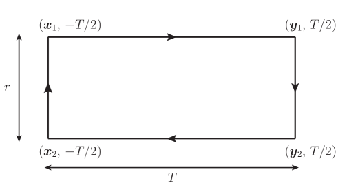
Figure 1: The rectangular Wilson loop.

We first consider the central potential from the instanton vacuum, restating briefly the results from Ref. Diakonov:1989un . The leading-order expectation value of the Wilson loop in Euclidean space is defined as

$$\langle W_{C}[A]\rangle=\int DA_{\mu}\mathrm{Tr}P\exp{\left(i\oint_{C}{\rm d}x_{\mu}A_{\mu}(x)\right)}e^{-\mathcal{S}_{\mathrm{YM}}}$$ (16)

where $S_{\mathrm{YM}}$ is the Yang-Mills action for the gluon field. The Wilson loop in the instanton medium can be written as

$$W_{C}[I,\bar{I}]=P\exp{\left(i\oint_{C}{\rm d}t\sum_{I,\bar{I}}a_{I,\bar{I}}\right)},$$ (17)

where $a_{I,\bar{I}}=\dot{x}_{\mu}A_{\mu}^{I,\bar{I}}(x)$. $I$ ($\bar{I})$ denotes the instanton (anti-instanton). $A_{\mu}^{I,\bar{I}}$ represent the instanton (anti-instanton) solutions of which the explicit expressions can be found in Appendix. The sum $\sum_{I,\bar{I}}a_{I,\bar{I}}$ stands for the superposition of $N_{+}$ instantons and $N_{-}$ anti-instantons for the classical gluon background field $\bar{A}_{\mu}$, which is written as

$$\dot{x}_{\mu}\bar{A}_{\mu}(x,\,\xi)=\sum_{I=1}^{N_{+}}a_{I}(x,\,\xi)+\sum_{\bar{I}=1}^{N_{-}}a_{\bar{I}}(x,\,\xi),$$ (18)

where $\xi$ represents the set of collective coordinates for the instanton, consisting of its center $z_{I\mu}$, the size $\rho_{I}$, and $\mathrm{SU}(N_{c})$ orientation matrix with the number of colors $N_{c}$. The integration over the gluon fields given in Eq. (16) is then replaced with the integrations over the set of collective coordinates of the instantons (anti-instantons) Diakonov:1983hh ; Diakonov:1985eg ; Diakonov:1989un such that Eq. (16) can be understood as an average over instanton ensemble.

The leading-order heavy-quark propagator in the rest frame is written in terms of the superposition of the instantons

$$S_{0}^{(i)}(x,y;a_{I,\bar{I}})=\langle y|\left(\frac{d}{dt}-\sum_{I,\bar{I}}a_{I,\bar{I}}^{(i)}+i\epsilon\right)^{-1}|x\rangle,$$ (19)

where $a_{I,\bar{I}}^{(i)}$ represents the gluon field projected onto the corresponding ith Wilson line. Since $T\to\infty$, we can neglect the short sides of the rectangular path. The separation between the two long Wilson lines is given as $r$, as shown in Fig. 1. Using Eqs.(12) and (19), we can write the Wilson loop along the rectangle shown in Fig. 1 as

$$\mathrm{Tr}W_{C}=\left\langle\kern-3.59999pt\left\langle\mathrm{Tr}\left[S_{0}^{(1)}(\bm{x}_{1},-T/2,\bm{y}_{1},T/2\;;a_{I,\bar{I}})S_{0}^{(2)}(\bm{x}_{2},-T/2,\bm{y}_{2},T/2\;;a_{I,\bar{I}})\rangle\right]\right\rangle\kern-3.59999pt\right\rangle,$$ (20)

The double angle bracket $\left\langle\kern-5.99998pt\left\langle\cdots\right\rangle\kern-5.99998pt\right\rangle$ emphasizes the average over the instanton ensemble. Each heavy-quark propagator in Eq. (20) is expanded in powers of the instanton and anti-instanton fields $a_{I,\bar{I}}^{(1,2)}$. Then the sum of the planar diagrams is carried out, which is the leading order in the $1/N_{c}$ expansion Pobylitsa:1989uq . Note that the instanton vacuum has two parameters characterizing the dilute instanton liquid Shuryak:1981ff ; Diakonov:1983hh : the average size of the instanton $\bar{\rho}\simeq 0.33\,\mathrm{fm}$ and the average separation between instantons $\bar{R}=(N/V)^{-1/4}\simeq 1\,\mathrm{fm}$, where the instanton density is given as $N/V\simeq(200\,\mathrm{MeV})^{4}$. It allows one to use $N/VN_{c}$ as a small perturbation parameter. We refer to Ref. Diakonov:1989un for further details of the calculation.

Using Eq. (73), we can obtain the explicit form of the central potential from the instanton vacuum as

$$V_{C} =\frac{N}{2VN_{c}}\int d^{3}z_{I}\mathrm{Tr}_{c}\left[1-P\exp\left(i\int_{-T/2}^{T/2}dx_{4}A_{I4}^{(1)}\right)P\exp\left(-i\int_{-T/2}^{T/2}dx_{4}A_{I4}^{(2)}\right)\right]_{z_{I4}=0}+(I\to\bar{I})$$ (21)

$$=\frac{2N}{VN_{c}}\int d^{3}z\left[1-\cos\left(\frac{\pi|\vec{z}|}{\sqrt{|\vec{z}|^{2}+\bar{\rho}^{\,2}}}\right)\cos\left(\frac{\pi|\vec{z}+\vec{r}|}{\sqrt{|\vec{z}+\vec{r}|^{2}+\bar{\rho}^{\,2}}}\right)\right.$$ (22)

$$\left.-\frac{\vec{z}(\vec{z}+\vec{r})}{|\vec{z}||\vec{z}+\vec{r}|}\sin\left(\frac{\pi|\vec{z}|}{\sqrt{|\vec{z}|^{2}+\bar{\rho}^{\,2}}}\right)\sin\left(\frac{\pi|\vec{z}+\vec{r}|}{\sqrt{|\vec{z}+\vec{r}|^{2}+\bar{\rho}^{\,2}}}\right)\right],$$ (23)

where $z$ denotes the position of the instanton, which is one of the collective coordinates for the instantons. The trace $\mathrm{Tr}_{c}$ runs over the colour space and $r$ is a distance between quark and antiquark. Further introducing the dimentionless variables $y=z/\bar{\rho}$ and $x=r/\bar{\rho}$, one can rewrite the potential in terms of the dimensionless integral $I(x)$

$$V_{C}(r) = \frac{4\pi N\bar{\rho}^{\,3}}{VN_{c}}\,I\left(\frac{r}{\bar{\rho}}\right),$$ (24)

$$I(x) = \int_{0}^{\infty}y^{2}dy\int_{-1}^{1}dt\,\left[1-\cos\left(\pi\frac{y}{\sqrt{y^{2}+1}}\right)\cos\left(\pi\sqrt{\frac{y^{2}+x^{2}+2xyt}{y^{2}+x^{2}+2xyt+1}}\,\right)\right.$$ (26)

$$\left.-\frac{y+xt}{\sqrt{y^{2}+x^{2}+2xyt}}\sin\left(\pi\frac{y}{\sqrt{y^{2}+1}}\right)\sin\left(\pi\sqrt{\frac{y^{2}+x^{2}+2xyt}{y^{2}+x^{2}+2xyt+1}}\,\right)\right].$$

As $r$ goes to infinity, the potential is saturated to be a constant

$$\lim_{r\to\infty}V_{C}(r)=2\Delta M_{Q},$$ (27)

where $\Delta M_{Q}$ is the correction to the heavy-quark mass from the instanton vacuum  Diakonov:1989un

$$\Delta M_{Q} =\frac{N}{2VN_{c}}\int d^{3}z\mathrm{Tr}_{c}\left[1-\left.P\exp\left(i\int\limits_{-\infty}^{\infty}dx_{4}A_{I4}\right)\right|_{z_{4}=0}\right]+(I\to\bar{I})$$ (28)

$$=\frac{8\pi N\bar{\rho}^{3}}{VN_{c}}\int\limits_{0}^{\infty}dy\,y^{2}\left(1+\cos\frac{\pi y}{\sqrt{y^{2}+1}}\right)=-\frac{4\pi^{4}N\bar{\rho}^{3}}{3VN_{c}}\left(J_{0}(\pi)+\frac{1}{\pi}J_{1}(\pi)\right)$$ (29)

calculated using again Eq. (73). The average size of the instanton is regarded as a renormalization scale of the instanton vacuum Diakonov:1985eg ; Son:2015bwa . Keeping in mind the fact that the current quark mass is scale-dependent and its value is usually given at $\mu=m_{c}$, certain scaling effects arising from the renormalization group equation for the quark mass should be taken into account in order to estimate the effects on the heavy-quark mass from the instanton vacuum. The instanton effects would be slightly decreased, when one matches the scale of $\Delta M_{Q}$ to the charmed quark mass given in Ref. PDG2016 .

We are now in a position to consider the spin-dependent parts of the heavy-quark potential. The general procedure is very similar to what was done in Eq. (20). Since we consider now the finite heavy-quark mass, we need to use the full propagator given in Eq. (13) instead of the leading one. That is, we calculate the two Wilson lines as

$$\mathrm{Tr}W_{C}=\left\langle\kern-3.59999pt\left\langle\mathrm{Tr}\left[S^{(1)}(\bm{x}_{2},-T/2,\bm{y}_{2},T/2\;;a_{I,\bar{I}})S^{(2)}(\bm{x}_{1},-T/2,\bm{y}_{1},T/2\;;a_{I,\bar{I}})\rangle\right]\right\rangle\kern-3.59999pt\right\rangle.$$ (30)

Considering the fact that $1/m_{Q}$ can be regarded as a small parameter, we can expand the full propagators in Eq. (30) iteratively in powers of $1/m_{Q}$. Using the relations given in Eq. (7), we first expand the term between $S_{0}$ and $S$ in powers of $1/m_{Q}$

$$i\not{D}_{\perp}\frac{1}{2m_{Q}+iv\cdot D}i\not{D}_{\perp}\approx\frac{1}{2m_{Q}}\left(-\bm{D}^{2}+\sigma\cdot\bm{B}\right)+\frac{1}{4m_{Q}^{2}}\left[\bm{E}\cdot\bm{D}+\bm{\sigma}\cdot(\bm{E}\times\bm{D})\right].$$ (31)

Then, the heavy-quark propagator for the $i$th Wilson loop can be iteratively expressed in powers of $1/m_{Q}$ as

$$S^{(i)}(x,y;A) \approx S_{0}^{(i)}(x,y;A)-\frac{1}{2m_{Q}}\int d^{4}\eta\,S_{0}^{(i)}(x,\eta;A)(-\bm{D}^{2}+\bm{\sigma}_{i}\cdot\bm{B})S_{0}^{(i)}(\eta,y;A)$$ (32)

$$-\frac{1}{4m_{Q}^{2}}\int d^{4}\eta\,S_{0}^{(i)}(x,\eta;A)(\bm{D}\cdot\bm{D}+\bm{\sigma}_{i}\cdot(\bm{E}\times\bm{D}))S_{0}^{(i)}(\eta,y;A)$$ (33)

$$+\frac{1}{4m_{Q}^{2}}\int d^{4}\eta d^{4}\eta^{\prime}\,\theta(\eta_{4}^{\prime}-\eta_{4})S_{0}^{(i)}(x,\eta;A)(-\bm{D}^{2}+\bm{\sigma}_{i}\cdot\bm{B})S_{0}^{(i)}(\eta,\eta^{\prime};A)$$ (34)

$$\hskip 85.35826pt\times\,(-\bm{D}^{2}+\bm{\sigma}_{i}\cdot\bm{B})S_{0}^{(i)}(\eta^{\prime},y;A).$$ (35)

Replacing the full propagator in Eq. (30) with Eq. (35), we obtain the following expression

$$\mathrm{Tr}W_{C} =\left\langle\kern-3.59999pt\left\langle\mathrm{Tr}\left[S_{0}^{(1)}(\bm{x}_{1},-T/2,\bm{y}_{1},T/2\;;a_{I,\bar{I}})S_{0}^{(2)}(\bm{x}_{2},-T/2,\bm{y}_{2},T/2\;;a_{I,\bar{I}})\rangle\right]\right\rangle\kern-3.59999pt\right\rangle$$ (36)

$$-\frac{1}{4m_{Q}^{2}}\int d^{4}\eta d^{4}\eta^{\prime}\,\left\langle\kern-3.59999pt\left\langle\mathrm{Tr}\left[S_{0}^{(1)}(\bm{x}_{1},-T/2,\bm{\eta},\eta_{4}\;;a_{I,\bar{I}})(-\bm{D}^{2}+\bm{\sigma}_{1}\cdot\bm{B})S_{0}^{(1)}(\bm{\eta},\eta_{4},\bm{y}_{1},T/2;a_{I,\bar{I}})\right.\right.\right.$$ (37)

$$\hskip 28.45274pt\times\,\left.\left.\left.S_{0}^{(2)}(\bm{x}_{2},-T/2,\bm{\eta},\eta_{4}\;;a_{I,\bar{I}})(-\bm{D}^{2}+\bm{\sigma}_{2}\cdot\bm{B})S_{0}^{(2)}(\bm{\eta},\eta_{4},\bm{y}_{1},T/2;a_{I,\bar{I}})\right]\right\rangle\kern-3.59999pt\right\rangle$$ (38)

$$-\frac{1}{4m_{Q}^{2}}\left\langle\kern-3.59999pt\left\langle\mathrm{Tr}\left[S_{0}^{(1)}(\bm{x}_{1},-T/2,\bm{y}_{1},T/2\;;a_{I,\bar{I}})\int d^{4}\eta\,S_{0}^{(2)}(\bm{x}_{2},-T/2,\bm{\eta},\eta_{4};a_{I,\bar{I}})(\bm{E}\cdot\bm{D}+\bm{\sigma}_{2}\cdot(\bm{E}\times\bm{D}))\right.\right.\right.$$ (39)

$$\left.\left.\left.\hskip 28.45274pt\times\,S_{0}^{(2)}(\bm{\eta},\eta_{4},\bm{y}_{2},T/2;a_{I,\bar{I}})\right]\right\rangle\kern-3.59999pt\right\rangle$$ (40)

$$-\frac{1}{4m_{Q}^{2}}\left\langle\kern-3.59999pt\left\langle\mathrm{Tr}\left[\int d^{4}\eta\,S_{0}^{(1)}(\bm{x}_{1}-T/2,\bm{\eta},\eta_{4};a_{I,\bar{I}})(\bm{E}\cdot\bm{D}+\bm{\sigma}_{1}\cdot(\bm{E}\times\bm{D}))S_{0}^{(1)}(\bm{\eta},\eta_{4},\bm{y}_{1},T/2;a_{I,\bar{I}})\right.\right.\right.$$ (41)

$$\left.\left.\left.\hskip 28.45274pt\times\,S_{0}^{(2)}(\bm{x}_{2},-T/2,\bm{y}_{2},T/2\;;a_{I,\bar{I}})\right]\right\rangle\kern-3.59999pt\right\rangle$$ (42)

$$+\frac{1}{4m_{Q}^{2}}\left\langle\kern-3.59999pt\left\langle\mathrm{Tr}\left[S_{0}^{(1)}(\bm{x}_{1}-T/2,\bm{y}_{1},T/2;a_{I,\bar{I}})\int d^{4}\eta d^{4}\eta^{\prime}\,S_{0}^{(2)}(\bm{x}_{2},-T/2,\bm{\eta},\eta_{4};a_{I,\bar{I}})(-\bm{D}^{2}+\bm{\sigma}_{2}\cdot\bm{B})\right.\right.\right.$$ (43)

$$\left.\left.\left.\hskip 28.45274pt\times S_{0}^{(2)}(\bm{\eta},\eta_{4},\bm{\eta}^{\prime},\eta_{4}^{\prime};a_{I,\bar{I}})(-\bm{D}^{2}+\bm{\sigma}_{2}\cdot\bm{B})S_{0}^{(2)}(\bm{\eta}^{\prime},\eta_{4}^{\prime},\bm{y}_{2},T/2;a_{I,\bar{I}})\right]\right\rangle\kern-3.59999pt\right\rangle$$ (44)

$$+\frac{1}{4m_{Q}^{2}}\left\langle\kern-3.59999pt\left\langle\mathrm{Tr}\left[\int d^{4}\eta d^{4}\eta^{\prime}\,S_{0}^{(1)}(\bm{x}_{1},-T/2,\bm{\eta},\eta_{4};a_{I,\bar{I}})(-\bm{D}^{2}+\bm{\sigma}_{1}\cdot\bm{B})S_{0}^{(1)}(\bm{\eta},\eta_{4},\bm{\eta}^{\prime},\eta_{4}^{\prime};a_{I,\bar{I}})\right.\right.\right.$$ (45)

$$\left.\left.\left.\hskip 28.45274pt\times\,(-\bm{D}^{2}+\bm{\sigma}_{1}\cdot\bm{B})S_{0}^{(1)}(\bm{\eta}^{\prime},\eta_{4}^{\prime},,\bm{y}_{1},T/2;a_{I,\bar{I}})S_{0}^{(2)}(\bm{x}_{2},-T/2,\bm{y}_{2},T/2;a_{I,\bar{I}})\right]\right\rangle\kern-3.59999pt\right\rangle.$$ (46)

Note that here we consider only the spin-dependent parts. For example, we can exclude the spin-independent term $\bm{D}^{2}/2m_{Q}$, which is just the kinetic energy, and that proportional to $\bm{\sigma}\cdot\bm{B}$, which disappears because of parity invariance Eichten:1980mw . We can further simplify Eq. (46), leaving all spin-independent parts out, which are just part of relativistic corrections to the potential. Taking only the spin-dependent parts into account, we obtain

$$\mathrm{Tr}W_{C}^{1/m_{Q}^{2}} =-\frac{1}{4m_{Q}^{2}}\int d^{4}\eta d^{4}\eta^{\prime}\,\left\langle\kern-3.59999pt\left\langle\mathrm{Tr}\left[S_{0}^{(1)}(\bm{x}_{1},-T/2,\bm{\eta},\eta_{4}\;;a_{I,\bar{I}})(-\bm{D}^{2})S_{0}^{(1)}(\bm{\eta},\eta_{4},\bm{y}_{1},T/2;a_{I,\bar{I}})\right.\right.\right.$$ (47)

$$\hskip 28.45274pt\times\,\left.\left.\left.S_{0}^{(2)}(\bm{x}_{2},-T/2,\bm{\eta},\eta_{4}\;;a_{I,\bar{I}})(\bm{\sigma}_{2}\cdot\bm{B})S_{0}^{(2)}(\bm{\eta},\eta_{4},\bm{y}_{1},T/2;a_{I,\bar{I}})\right]\right.\right.$$ (48)

$$\hskip 79.6678pt+\left.\left.\mathrm{Tr}\left[S_{0}^{(1)}(\bm{x}_{1},-T/2,\bm{\eta},\eta_{4}\;;a_{I,\bar{I}})(\bm{\sigma}_{1}\cdot\bm{B})S_{0}^{(1)}(\bm{\eta},\eta_{4},\bm{y}_{1},T/2;a_{I,\bar{I}})\right.\right.\right.$$ (49)

$$\hskip 28.45274pt\times\,\left.\left.\left.S_{0}^{(2)}(\bm{x}_{2},-T/2,\bm{\eta},\eta_{4}\;;a_{I,\bar{I}})(-\bm{D}^{2})S_{0}^{(2)}(\bm{\eta},\eta_{4},\bm{y}_{1},T/2;a_{I,\bar{I}})\right]\right\rangle\kern-3.59999pt\right\rangle$$ (50)

$$\hskip 79.6678pt+\left.\left.\mathrm{Tr}\left[S_{0}^{(1)}(\bm{x}_{1},-T/2,\bm{\eta},\eta_{4}\;;a_{I,\bar{I}})(\bm{\sigma}_{1}\cdot\bm{B})S_{0}^{(1)}(\bm{\eta},\eta_{4},\bm{y}_{1},T/2;a_{I,\bar{I}})\right.\right.\right.$$ (51)

$$\hskip 28.45274pt\times\,\left.\left.\left.S_{0}^{(2)}(\bm{x}_{2},-T/2,\bm{\eta},\eta_{4}\;;a_{I,\bar{I}})(\bm{\sigma}_{2}\cdot\bm{B})S_{0}^{(2)}(\bm{\eta},\eta_{4},\bm{y}_{1},T/2;a_{I,\bar{I}})\right]\right\rangle\kern-3.59999pt\right\rangle$$ (52)

$$-\frac{1}{4m_{Q}^{2}}\left\langle\kern-3.59999pt\left\langle\mathrm{Tr}\left[S_{0}^{(1)}(\bm{x}_{1},-T/2,\bm{y}_{1},T/2\;;a_{I,\bar{I}})\right.\right.\right.$$ (53)

$$\left.\left.\left.\hskip 28.45274pt\times\,\int d^{4}\eta\,S_{0}^{(2)}(\bm{x}_{2},-T/2,\bm{\eta},\eta_{4};a_{I,\bar{I}})(\bm{\sigma}_{2}\cdot(\bm{E}\times\bm{D}))S_{0}^{(2)}(\bm{\eta},\eta_{4},\bm{y}_{2},T/2;a_{I,\bar{I}})\right]\right\rangle\kern-3.59999pt\right\rangle$$ (54)

$$-\frac{1}{4m_{Q}^{2}}\left\langle\kern-3.59999pt\left\langle\mathrm{Tr}\left[\int d^{4}\eta\,S_{0}^{(1)}(\bm{x}_{1}-T/2,\bm{\eta},\eta_{4};a_{I,\bar{I}})(\bm{\sigma}_{1}\cdot(\bm{E}\times\bm{D}))S_{0}^{(1)}(\bm{\eta},\eta_{4},\bm{y}_{1},T/2;a_{I,\bar{I}})\right.\right.\right.$$ (55)

$$\left.\left.\left.\hskip 28.45274pt\times\,S_{0}^{(2)}(\bm{x}_{2},-T/2,\bm{y}_{2},T/2\;;a_{I,\bar{I}})\right]\right\rangle\kern-3.59999pt\right\rangle.$$ (56)

The final expression for $W_{C}^{1/m_{Q}^{2}}$ contains $1/m_{Q}^{2}$, so that we can expand the exponential of Eq. (14) in powers of $1/m_{Q}^{2}$. Then, Eq. (56) will lead to the spin-dependent parts of the heavy-quark potential from the instanton vacuum. The derivation of the potential from Eq. (56) is lengthy but straightforward. In Ref. Eichten:1980mw , it was shown in very detail how one can obtain the spin-dependent parts of the heavy-quark potential in QCD. Since the form of Eq. (56) is very similar to the corresponding one in Ref. Eichten:1980mw , we will closely follow the method of Ref. Eichten:1980mw and refer to it. The leading-order propagator given in Eq. (12) is identified as the path-order exponential along the time direction apart from the Dirac delta function. Using the identities for the path-ordered exponentials given in Appendix, we can proceed to compute each term in Eq. (56). Note that the instanton satisfies the self-duality condition $G_{\mu\nu}^{a}=\pm\tilde{G}_{\mu\nu}^{a}$ ($\bm{B}=\pm\bm{E}$), which plays an essential role in deriving the spin-dependent potential from the instanton vacuum. It makes it possible to relate several independent potentials to the central potential given in Eq.(24). As a result, all the spin-dependent potentials are expressed in terms of the central potential

$$V_{SD}(\bm{r}) =\frac{1}{4m_{Q}^{2}}\left(\bm{L}_{1}\cdot\bm{\sigma}_{2}-\bm{L}_{2}\cdot\bm{\sigma}_{1}\right)\frac{1}{r}\frac{dV_{C}(r)}{dr}+\frac{\bm{\sigma}_{1}\cdot\bm{\sigma}_{2}}{12m_{Q}^{2}}\nabla^{2}V_{C}(r)$$ (57)

$$\hskip 28.45274pt+\frac{1}{3m_{Q}^{2}}(3\bm{\sigma}_{1}\cdot\bm{n}\,\bm{\sigma}_{2}\cdot\bm{n}-\bm{\sigma}_{1}\cdot\bm{\sigma}_{2})\left(\frac{1}{r}\frac{d}{dr}-\frac{d^{2}}{dr^{2}}\right)V_{C}(r),$$ (58)

where $\bm{L}_{i}$ and $\bm{\sigma}_{i}$ represent respectively the orbital angular momentum and the Pauli spin operator of the corresponding heavy quark, $\bm{n}$ designates the unit radial vector. The potential $V_{C}(r)$ denotes the central part of the potential that we already have shown in Eq. (24). We want to mention that we have used $m_{Q}=m_{\bar{Q}}$. If one considers two heavy quarks with different masses, we can simply replace $m_{Q}^{2}$ with $m_{Q}m_{\bar{Q}}$ in Eq. (58).

The spin-dependent potential $V_{SD}$ can be now decomposed into three different parts, i.e., the spin-spin interaction $V_{SS}(r)$, the spin-orbit coupling term $V_{LS}(r)$, and the tensor part $V_{T}(r)$:

$$V_{Q\bar{Q}}(\bm{r})=V_{C}(r)+V_{SS}(r)(\bm{S}_{Q}\!\cdot\!\bm{S}_{\bar{Q}})+V_{LS}(r)(\bm{L}\cdot\bm{S})+V_{T}(r)\left[3(\bm{S}_{Q}\!\cdot\!\bm{n})(\bm{S}_{\bar{Q}}\!\cdot\!\bm{n})-\bm{S}_{Q}\cdot\bm{S}_{\bar{Q}}\right],$$ (59)

where $\bm{S}_{Q({\bar{Q}})}$ stands for the spin of a heavy quark (heavy anti-quark) $\bm{S}_{Q({\bar{Q}})}=\bm{\sigma}_{1(2)}/2$, $\bm{S}$ does their total spin $\bm{S}=\bm{S}_{1}+\bm{S}_{2}$, and $\bm{L}$ represents the relative orbital angular momentum $\bm{L}=\bm{L}_{1}-\bm{L}_{2}$. Each potential of Eq. (59) is defined respectively as

$$V_{SS}(r)=\frac{1}{3m_{Q}^{2}}\nabla^{2}V_{C}(r),\;\;\;\;V_{LS}(r)=\frac{1}{2m_{Q}^{2}}\frac{1}{r}\frac{dV_{C}(r)}{dr},\;\;\;\;V_{T}(r)=\frac{1}{3m_{Q}^{2}}\left(\frac{1}{r}\frac{dV_{C}(r)}{dr}-\frac{d^{2}V_{C}(r)}{dr^{2}}\right).$$ (60)

Thus, all three components of the spin-dependent potential are expressed in terms of the central potential $V_{C}(r)$.

III Numerical calculations, results and discussions

III.1 Instanton potential

In the instanton liquid model for the QCD vacuum, we have two important parameters, i.e., the average size of the instanton $\bar{\rho}\simeq 0.33\,\mathrm{fm}$ and the average distance $\bar{R}\simeq 1\,\mathrm{fm}$ between instantons, as we have already mentioned. These numbers were first proposed by Shuryak Shuryak:1981ff within the instanton liquid model and were derived from $\Lambda_{\overline{MS}}$ by Diakonov and Petrov Diakonov:1983hh . Thus, it is also of great interest to look into the dependence of the heavy-quark potential from the instanton vacuum on these parameters. Moreover, the values given above should not be considered as the exact ones. For example, Refs. Kim:2005jc ; Goeke:2007bj ; Goeke:2007nc considered $1/N_{c}$ meson-loop contributions in the light-quark sector and found it necessesary to readjust the values of parameters as $\bar{\rho}\simeq 0.35\,\mathrm{fm}$ and $\bar{R}\simeq 0.856\,\mathrm{fm}$. Lattice simulations of the instanton vacuum suggested $\bar{\rho}\approx 0.36\,\mathrm{fm}$ and $\bar{R}\approx 0.89\,\mathrm{fm}$ Chu:1994vi ; Negele:1998ev ; DeGrand:2001tm ; Faccioli:2003qz , which is almost the same as those with the $1/N_{c}$ meson-loop corrections. Thus, we want to examine the dependence of the heavy-quark potential from the instanton vacuum on three different sets of parameters, that is, Set I Diakonov:1983hh ; Shuryak:1981ff , Set IIa Kim:2005jc ; Goeke:2007bj ; Goeke:2007nc , and Set IIb Chu:1994vi ; Negele:1998ev ; DeGrand:2001tm ; Faccioli:2003qz . The parameter dependence of the potential can be easily understood from the form of leading-order potential expressed in Eq. (24). While the prefactor $\bar{\rho}^{3}/\bar{R}^{4}N_{c}$, which includes both the parameters, governs the overall strength of the potential, its range is dictated only by the instanton size $\bar{\rho}$ through the dimensionless integral $I(r/\bar{\rho})$.

When the quark-antiquark distance is smaller than the instanton size, i.e., $r\ll\bar{\rho}$ ($x\ll 1$), one can expand the dimensionless integral $I(x)$ with respect to $x$

$$I(x) \simeq\left[\frac{\pi^{3}}{48}-\frac{\pi^{3}}{3}J_{1}(2\pi)\right]x^{2}+\left[-\frac{\pi^{3}(438+7\pi^{2})}{30720}+\frac{J_{2}(2\pi)}{80}\right]x^{4}+{\cal O}(x^{6}),$$ (61)

which yields the central potential in the form of a polynomial

$$V_{C}(r)\simeq\frac{4\pi\bar{\rho}^{\,3}}{\bar{R}^{4}N_{c}}\,\left(1.345\,\frac{r^{2}}{\bar{\rho}^{2}}-0.501\,\frac{r^{4}}{\bar{\rho}^{4}}\right).$$ (62)

As the distance between the quark and the antiquark grows larger than the intstanton size, i.e. $r\gg\bar{\rho}$ ($x\gg 1$), we again get an analytic expression as follows

$$I(x)\simeq-\frac{2\pi^{2}}{3}\Big{[}\pi J_{0}(\pi)+J_{1}(\pi)\Big{]}-\frac{\pi^{2}}{2x}+{\cal O}(x^{-2})\,.$$ (63)

Consequently, the central potential at large $r$ can be approximately written as

$$V(r)\simeq 2\Delta M_{Q}-\frac{g_{\rm NP}}{r}.$$ (64)

The second term behaves like the Coulomb-like potential. So, crudely speaking, this can be understood as a nonperturbative contribution to the perturbative one gluon exchange potential from the instanton vauum at large $r$. The coupling constant $g_{\mathrm{NP}}$ in Eq.(64), which is defined as $g_{\rm NP}:=2\pi^{3}\bar{\rho}^{4}/(N_{c}\bar{R}^{4})$, could be regarded as a nonperturbative correction to the strong coupling constant $\alpha_{s}(r)$. When $r$ goes to infinity $r\rightarrow\infty$, the potential is saturated at the value of $2\Delta M_{Q}$. As discussed already in Ref. Diakonov:1989un , it implies that the instanton vacuum can not explain quark confinement. In the case of parameter Set I, which is often considered in the light-quark sector, the value of $\Delta M_{Q}$ is obtained to be $\Delta M_{Q}\simeq 66.6\,\mathrm{MeV}$. However, if one chooses Set IIa, then the result becomes $\Delta M_{Q}\simeq 143.06\,\mathrm{MeV}$. The Set IIb produces $\Delta M_{Q}\simeq 135.72\,\mathrm{MeV}$.

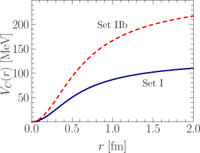
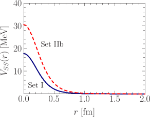
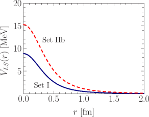
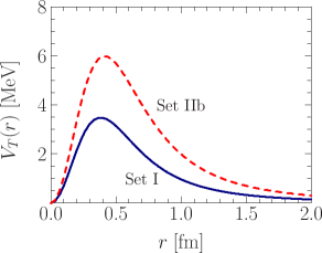
Figure 2: Each contribution to the heavy-quark potential as a function of $r$ for the two different sets of the instanton parameters $\bar{\rho}$ and $\bar{R}$. The upper-left panel depicts the central part of the potential, the upper-right panel draws the spin-spin interaction, the lower-left panel illustrates the spin-orbit part, and the lower-right one shows the tensor interaction. The solid curve corresponds to Set I with $\rho=0.33$ fm and $\bar{R}=1\,\mathrm{fm}$ from the phenomenolgy Shuryak:1981ff ; Diakonov:1983hh , whereas the dashed one corresponds to Set IIb with $\rho=0.36$ fm and $\bar{R}=0.89\,\mathrm{fm}$ from the lattice simulations Chu:1994vi ; Negele:1998ev ; DeGrand:2001tm ; Faccioli:2003qz . The mass of the charm quark is chosen to be $m_{c}=1275$ MeV.

Figure 2 draws $r$ dependence of each term of the heavy-quark potentials from the instanton vacuum. We take into account the charm quark sector as an example. We also show the dependence of each term of the potential on two different sets of parameters, that is, Set I and Set IIb. One can see that the central part of the potential increases monotonically at small distances $r\ll\bar{\rho}$ and later becomes almost linear at the distances comparable with the instanton size $r\sim\bar{\rho}$ as already discussed in Ref. Diakonov:1989un . At large $r\gg\bar{\rho}$ it starts to get saturated at the value $V_{C}(r\rightarrow\infty)\simeq 133.2$ MeV with Set I and $V_{C}(r\rightarrow\infty)\simeq 271.44$ MeV with Set IIb. The spin-spin interaction part is of particular interest among these contributions to the spin-dependent potential. In pQCD, it is given as a point-like interaction Brambilla:2004jw in the leading order. On the other hand, the spin-spin interaction from the instanton vacuum looks similar to a Gaussian-type interaction. The spin-orbit potential behaves in a similar way to the spin-spin potential. The tensor interaction, however, shows a different $r$ dependence. As $r$ increases, the tensor potential vanishes at $r=0$ and then starts to increase until $r\approx 0.4\,\mathrm{fm}$, from which it begins to fall off. The strength of each part of the potential become stronger when smaller value of $\bar{R}$ is employed, since all terms turn out to be very sensitive to $\bar{R}$ on account of the prefactor $\bar{\rho}^{3}/\bar{R}^{4}N_{c}$. It implies that a less dilute instanton medium yields stronger interactions between a heavy quark and a heavy antiquark. However, one has to keep in mind that the value of $\bar{R}$ should not be continually decreased, because the whole framework of the instanton liquid model is based on the diluteness of the instanton medium where the packing parameter proportional to $(\bar{\rho}/\bar{R})^{4}$ must be kept as a small parameter.

On the other hand, the change of the $\bar{\rho}$ value seems less effective in the spin-dependent parts of the potential. This is again due to the fact that all spin dependent parts have the prefactor $\bar{\rho}/\bar{R}^{4}N_{c}$ where instanton size appears in the first order, after rewriting the spin-dependent parts in terms of the dimensionless integral $I(x)$ (see Eq. (26)) and its derivatives. As mentioned in the previous section, the average size of the instanton has a physical meaning of the renormalization scale Diakonov:1985eg ; Son:2015bwa , which is a crucial virtue of the instanton liquid model. Thus, $\bar{\rho}=0.33\,\mathrm{fm}$ indicates the renormalization scale $\mu=600\,\mathrm{MeV}$. Bearing in mind this meaning of $\bar{\rho}$, we should not take the value of $\bar{\rho}$ freely. Note that the value of $\bar{\rho}^{-1}=600\,\mathrm{MeV}$ implies the strong couipling constant frozen at $\bar{\rho}^{-1}$. Thus, Fig. 2 shows the dependence of the heavy-quark potential on both $\bar{\rho}$ and $\bar{R}$ within a constraint range of their values. In the case of the bottom quarks and anti-quarks, the instanton effects are quite much suppressed because of the large bottom quark mass.

For completeness, we provide the expression for the matrix elements of $Q\bar{Q}$ potential in Eq. (59)

$$\langle{}^{2S+1}L_{J}|V_{Q\bar{Q}}(\bm{r})|{}^{2S+1}L_{J}\rangle =V(r)+\left[\frac{1}{2}S(S+1)-\frac{3}{4}\right]V_{SS}(r)+\frac{1}{2}\left[J(J+1)-L(L+1)-S(S+1)\right]V_{LS}(r)$$ (65)

$$\left\{-\frac{3\left[J(J+1)-L(L+1)-S(S+1)\right]\left[J(J+1)-L(L+1)-S(S+1)+1\right]}{2(2L-1)(2L+3)}\right.$$ (66)

$$\left.+\frac{2S(S+1)L(L+1)}{(2L-1)(2L+3)}\right\}V_{T}(r),$$ (67)

where we have used the conventional spectroscopic notation ${}^{2S+1}L_{J}$ given in terms of the total spin $S$, the orbital angular momentum $L$, and the total angular momentum $J$ satisfying the relation $\bm{J}=\bm{L}+\bm{S}$.

III.2 Gaussian Expansion Method

In order to evaluate the bound states in the spectrum of quarkonia, we need to solve the Schrödinger equation with the potential from the instanton vacuum given in Eq. (59)

$$\left[-\frac{\hbar^{2}}{m_{Q}}\nabla^{2}+V_{Q\bar{Q}}(\bm{r})-E\right]\Psi_{JM}(\bm{r})=0,$$ (68)

where $m_{Q}$ arises from the doubled reduced mass of the quarkonium system and $\Psi_{JM}$ represents the wave function of the state with the total angular momentum $J$ and its third component $M$. We can solve Eq.(68) numerically, using the Gaussian expansion method (see review Hiyama2003 ) in which the wave function is expanded in terms of a set of $L^{2}$-integrable basis functions $\{\Phi_{JM,n}^{LS};\,n=1-n_{\mathrm{max}}\}$

$$\Psi_{JM}(\bm{r})=\sum_{n=1}^{n_{\rm max}}C_{n,LS}^{(J)}\Phi_{JM,n}^{LS}(\bm{r})$$ (69)

and the Rayleigh-Ritz variational principle is employed. Thus, one can formulate a generalized eigenvalue problem given as

$$\sum_{m=1}^{n_{\rm max}}\langle\Phi_{JM,n}^{LS}\left|-\frac{\hbar^{2}}{m_{Q}}\nabla^{2}+V_{Q\bar{Q}}(\bm{r})-E\right|\Phi_{JM,m}^{LS}\rangle C_{m,LS}^{(J)}=0\,.$$ (70)

The normalized radial part of the basis wave functions $\phi_{n}^{L}(r)$ is expressed in terms of the Gaussian basis functions

$$\phi_{n}^{L}(r)=\left(\frac{2^{2L+\frac{7}{2}}r_{n}^{-2L-3}}{\sqrt{\pi}(2L+1)!!}\right)^{1/2}r^{L}e^{-(r/r_{n})^{2}},$$ (71)

where $r_{n},\,n=1,2,...,n_{max}$ stand for variational parameters. In the case of a two-body problem, the total number of the variational parameters can be reduced by choosing the geometric progression in the form of $r_{n}=r_{1}a^{n-1}$, which produces a good convergence of the results. Thus, we need only three variational parameters, i.e. $r_{1}$, $a$ and $n_{\mathrm{max}}$.

III.3 Quarkonium states

We already mentioned that at large distance the instanton potential is saturated, so that there is no confinement in the present approach. The bound or quasibound charmonium states with the masses below or around the threshold mass $M_{Q\bar{Q}}\simeq 2(m_{c}+\Delta M_{Q})$, where $m_{c}=1275$ is the charm quark mass PDG2016 , are listed in Table 1 with the two different sets of the instanton parameters. Other states above threshold will appear as resonances in the present approach.

	This work	This work
	Set I	Set IIb	Experiment PDG2016
	$\bar{\rho}=1/3$ fm, $R=1$ fm Shuryak:1981ff ; Diakonov:1983hh	$\bar{\rho}=0.36$ fm, $R=0.89$ fm Chu:1994vi ; Negele:1998ev ; DeGrand:2001tm ; Faccioli:2003qz	[MeV]
	[MeV]	[MeV]
$M_{\eta_{c}}$	2668.81	2753.64	$2983.6\pm 0.6$
$M_{J/\psi}$	2669.57	2755.36	$3096.916\pm 0.11$
$M_{\chi_{c0}}$	2692.43	2800.86	$3414.75\pm 0.31$
$M_{\chi_{c1}}$	2692.50	2801.11	$3510.66\pm 0.07$
$M_{\chi_{c2}}$	2692.67	2801.70	$3556.20\pm 0.09$

Table 1: Low-lying charmonium states from the instanton potential. Charm quark mass is set to be $m_{c}=1275$ MeV.

One can see that the instanton effects are not small in reproducing the mass of quarkonia. For example, in the case of the potential with parameter Set I, the contribution to the mass of a charmonium is determined by $\Delta M_{c\bar{c}}=M_{c\bar{c}}-2m_{c}$. For example, the contribution of the instanton effects to the $\eta_{c}$ mass turns out to be $118.81\,\mathrm{MeV}$, which is approximately about $30\,\%$ in comparison with the experimental data 433.60 MeV. As discussed already, the potential from the instanton vacuum is sensitive to the instanton parameters. Therefore, the change in the instanton parameters strongly affects the spectrum of $Q\bar{Q}$ states. For example, parameter Set IIb gives the result $\Delta M_{\eta_{c}}\simeq 203.64$ MeV, which is almost $50\,\%$, compared to the data. Parameter Set IIa gives slightly larger results than those with Set IIb. When it comes to the $J/\psi$ state, the instanton effects on the $Q\bar{Q}$ mass becomes smaller in comparison with the experimental data. However, it is still important to consider them, since $\Delta M_{J/\psi}$ is 119.57 MeV (205.36 MeV) with Set I (Set IIb) used, compared with the data 540.92 MeV. On the other hand, we obtain $\Delta M_{\chi_{c0}}\simeq 142.43$ MeV (Set I) and $\Delta M_{\chi_{c0}}\simeq 250.86$ MeV (Set IIb). Parameter Set I reproduces $\chi_{c0}$, $\chi_{c1}$ and $\chi_{c2}$ as quasibound states while parameter Set IIb yields them as the definite bound states.

It is of also interest to discuss the effects of the hyperfine mass splitting from the instanton vacuum. The contribution to the hyperfine mass splitting of each low-lying charmonium state is listed in Table 2.

	This work	This work
	Set I	Set IIb	Experiment  PDG2016
	$\bar{\rho}=1/3$ fm, $R=1$ fm Shuryak:1981ff ; Diakonov:1983hh	$\bar{\rho}=0.36$ fm, $R=0.89$ fm Chu:1994vi ; Negele:1998ev ; DeGrand:2001tm ; Faccioli:2003qz	[MeV]
	[MeV]	[MeV]
$\Delta M_{J/\psi-\eta_{c}}$	0.72	1.72	113.32 $\pm$ 0.70
$\Delta M_{\chi_{c1}-\chi_{c0}}$	0.07	0.25	95.91 $\pm$ 0.32
$\Delta M_{\chi_{c2}-\chi_{c0}}$	0.24	0.84	141.45 $\pm$ 0.32
$\Delta M_{\chi_{c2}-\chi_{c1}}$	0.16	0.59	45.54 $\pm$ 0.11

Table 2: Contributions to the hyperfine mass splittings of the low-lying charmonium states. Charm quark mass is set to be $m_{c}=1275$ MeV.

While the instanton effects come into play significantly on $\Delta M_{c\bar{c}}$, they turn out to be rather small in describing the hyperfine mass splittings of the charmonia. This might be due to the fact that the spin-dependent part of the potential from the instanton vacuum is almost an order of magnitude smaller than the central part. The tensor interaction almost does not contribute to the results. As a result, the instanton effects on the hyperfine mass splittings are almost negligible. In order to obtain realistic results of the hyperfine mass splittings as well as of the charmonium masses, we need to include the Coulomb-like potential coming from the perturbative one gluon-exchange and the confining potential together with that from the instanton vacuum.

	This work
	Set I	Experiment PDG2016
	$\bar{\rho}=1/3$ fm, $R=1$ fm Shuryak:1981ff ; Diakonov:1983hh	[MeV]
	[MeV]
$M_{\eta_{b}}$	8454.58	$9399.0\pm 2.3$
$M_{\Upsilon}$	8454.76	$9460.30\pm 0.26$
$M_{\chi_{b0}}$	8477.95	$9859.44\pm 0.52$
$M_{\chi_{b1}}$	8477.97	$9892.78\pm 0.40$
$M_{\chi_{b2}}$	8478.01	$9912.21\pm 0.40$

Table 3: Low-lying bottomonium states from the instanton potential. Charm quark mass is set to be $m_{b}=4180$ MeV.

IV Summary and outlook

In the present work, we aimed at investigating the instanton effects on the heavy-quark potential, based on the instanton liquid model. We first considered the heavy-quark propagator starting from the QCD Lagrangian, which comes into an essential play in deriving the heavy-quark potential. We showed briefly how to construct the heavy-quark potential from the instanton vacuum. Expanding the heavy-quark propagator in powers of the inverse mass of the heavy quark, we obtained the spin-dependent parts of the heavy-quark potential. We studied the dependence of the heavy-quark potential on the two essential parameters for the instanton vacuum, that is, the average size of the instanton $(\bar{\rho})$ and the inter-distance between the instantons $(\bar{R})$. The results of the potential are very sensitive to the parameter $\bar{R}$, while they are varied marginally with $\bar{\rho}$ changed. The spin-spin interaction shows $r$ dependence similar to a Gaussian-type potential, which is distinguished from the point-like spin-spin interaction derived from perturbative QCD. The spin-orbit potential behaves like the spin-spin interaction, whereas the tensor potential exhibits a different character. It increases until $r$ reaches approximately $0.4$ fm and then starts to fall off.

Having solved explicitly the Schrödinger equation with the heavy-quark potential purely induced by the instantons, we discussed the masses of the low-lying quakonia. The instanton contribution to the hyperfine mass splitting turns out to be tiny due to smallness of the spin-dependent part of the potential. We also discussed the dependence of the results on the intrinsic parameters of the instanton vacuum, i.e. the average size of the instanton and the inter-distance between instantons.

It is of great importance to study carefully the mass spectra of the quarkonia and their decays by solving explicitly the Schrödinger equation, combining the heavy-quark potential derived in the present work with the confining and Coulomb potentials. Considering the fact that the instanton vacuum plays a key role in realizing chiral symmetry and its spontaneous breaking in QCD, the nonperturbative gluon dynamics is expected to shed light on strong decays of the quarkonia involving pions. Since the central part of the heavy-quark potential was derived by using the small packing parameter $N/VN_{c}$, we can obtain the corrections from the next-to-leading order $(N/VN_{c})^{2}$. In principle, it is not that difficult to compute them. Starting from the instanton operator corresponding to the Wilson line (see Eq.(17) in Ref. Diakonov:1989un ), we can consider the next-to-leading order in the expansion with respect to the small packing parameter of the instanton medium. Though the corrections from the next-to-leading order might be very small, one could use it for the fine-tuning of the mass spectrum of the quarkonia. The corresponding investigations are under way.

Appendix A Useful formulae

Using the instanton and anti-instanton fields

$$A_{I\mu}=\frac{x_{\nu}\bar{\eta}_{\mu\nu}^{a}\tau^{a}\rho^{2}}{x^{2}(x^{2}+\rho^{2})},\qquad A_{{\bar{I}}\mu}=\frac{x_{\nu}{\eta}_{\mu\nu}^{a}\tau^{a}\rho^{2}}{x^{2}(x^{2}+\rho^{2})},$$ (72)

where $\bar{\eta}_{\mu\nu}^{a}$ and ${\eta}_{\mu\nu}^{a}$ denote the ’t Hooft symbols 'tHooft:1976fv , we can easily derive the path-ordered exponential as follows Diakonov:1989un

$$P\exp\left(i\int_{-\infty}^{\infty}dx_{4}A_{I4}\right)=-\cos\left(\frac{\pi|\bm{z}|}{\sqrt{\rho^{2}+z^{2}}}\right)-i\frac{\bm{\tau}\cdot\bm{z}}{|\bm{z}|}\sin\left(\frac{\pi|\bm{z}|}{\sqrt{\rho^{2}+z^{2}}}\right),$$ (73)

which was used for deriving the heavy-quark potential and the instanton corrections to the heavy-quark mass.

The leading-order propagator given in Eq. (12) is the same as the path-ordered exponential apart from the Dirac delta function. Thus, it is of great use to consider the identities derived in Ref. Eichten:1980mw for the path-order exponentials when we compute the spin-dependent parts of the heavy-quark potential. Defining the path-ordered exponential as

$$P(x_{4},y_{4}):=P\exp\left(i\int_{x_{4}}^{y_{4}}dz_{4}A_{4}(z)\right),$$ (74)

we have the following identities

$$P(x_{4},y_{4})P(y_{4},z_{4})=P(x_{4},z_{4}),$$ (75)

$$D_{i}(x_{4})P(x_{4},y_{4})-P(x_{4},y_{4})D^{i}(y_{4})=\int_{y_{4}}^{x_{4}}dzP(x_{4},z)E_{i}(z)P(z,y_{4}),$$ (76)

$$P(\bm{y},t;\bm{x},t)D_{i}(\bm{x},t)P(\bm{x},t;\bm{y},t)=D_{i}(\bm{y},t)-\epsilon_{ijk}\int_{0}^{1}d\alpha(x-y)_{j}[P(\bm{y},t;\bm{z},t)B_{k}(\bm{z},t)P(\bm{z},t;\bm{y},t)],$$ (77)

where $\bm{z}=\alpha\bm{y}+(1-\alpha)\bm{x}$. $D_{i}$ denotes the spatial component of the covariant derivative. When time $t$ goes to infinity, i.e. $t=\pm\frac{T}{2}\to\infty$, the third identity is simplified to be

$$\lim_{|t|\to\infty}P(\bm{y},t;\bm{x},t)\bm{D}(\bm{x},t)P(\bm{x},t;\bm{y},t)=i\nabla_{y}.$$ (78)

References

- (1) S. K. Choi et al. [Belle Collaboration], Phys. Rev. Lett., 91: 262001 (2003)
- (2) B. Aubert et al. [BaBar Collaboration], Phys. Rev. D, 71: 071103 (2005)
- (3) B. Aubert et al. [BaBar Collaboration], Phys. Rev. Lett., 95: 142001 (2005)
- (4) K. Abe et al. [Belle Collaboration], Phys. Rev. Lett., 98: 082001 (2007)
- (5) S. K. Choi et al. [Belle Collaboration], Phys. Rev. Lett., 100: 142001 (2008)
- (6) A. Bondar et al. [Belle Collaboration], Phys. Rev. Lett., 108: 122001 (2012)
- (7) Z. Q. Liu et al. [Belle Collaboration], Phys. Rev. Lett., 110: 252002 (2013)
- (8) M. Ablikim et al. [BESIII Collaboration], Phys. Rev. Lett., 110: 252001 (2013)
- (9) M. Ablikim et al. [BESIII Collaboration], Phys. Rev. Lett., 111: 242001 (2013)
- (10) R. Aaij et al. [LHCb Collaboration], Phys. Rev. Lett., 110: 222001 (2013)
- (11) M. Ablikim et al. [BESIII Collaboration], Phys. Rev. Lett., 112: 022001 (2014)
- (12) R. Aaij et al. [LHCb Collaboration], Phys. Rev. Lett., 112: 222002 (2014)
- (13) R. Aaij et al. [LHCb Collaboration], Phys. Rev. D, 92: 112009 (2015)
- (14) B. Aubert et al. [BaBar Collaboration], Phys. Rev. Lett., 101: 071801 (2008) [Phys. Rev. Lett., 102: 029901 (2009)]
- (15) B. Aubert et al. [BaBar Collaboration], Phys. Rev. Lett., 103: 161801 (2009)
- (16) G. Bonvicini et al. [CLEO Collaboration], Phys. Rev. D, 81: 031104 (2010)
- (17) R. Mizuk et al. [Belle Collaboration], Phys. Rev. Lett., 109: 232002 (2012)
- (18) S. Dobbs, Z. Metreveli, K. K. Seth, A. Tomaradze and T. Xiao, Phys. Rev. Lett., 109: 082001 (2012)
- (19) U. Tamponi et al. [Belle Collaboration], Phys. Rev. Lett., 115: 142001 (2015)
- (20) R. Mizuk et al. [Belle Collaboration], Phys. Rev. Lett., 117: 142001 (2016)
- (21) R. Aaij et al. [LHCb Collaboration], Phys. Rev. Lett., 115: 072001 (2015)
- (22) A. J. Bevan et al. [BaBar and Belle Collaborations], Eur. Phys. J. C, 74: 3026 (2014)
- (23) A. Andronic et al., Eur. Phys. J. C, 76: 107 (2016)
- (24) C. Z. Yuan [BESIII Collaboration], Front. Phys. China, 10: 101401 (2015)
- (25) C. Z. Yuan [Belle Collaboration], arXiv:1512.03281 [hep-ex]
- (26) E. S. Swanson, Phys. Rept., 429: 243 (2006).
- (27) E. Eichten, S. Godfrey, H. Mahlke and J. L. Rosner, Rev. Mod. Phys., 80: 1161—1193 (2008)
- (28) M. B. Voloshin, Prog. Part. Nucl. Phys., 61: 455—511 (2008)
- (29) N. Brambilla et al., Eur. Phys. J. C, 71: 1534 (2011)
- (30) S. L. Olsen, Front. Phys., 10: 101401 (2015)
- (31) A. A. Penin, arXiv:0905.4296 [hep-ph].
- (32) S. Recksiegel and Y. Sumino, Phys. Lett. B, 578: 369—375 (2004)
- (33) B. A. Kniehl, A. A. Penin, A. Pineda, V. A. Smirnov and M. Steinhauser, Phys. Rev. Lett., 92: 242001 (2004) [Phys. Rev. Lett., 104: 242001 (2010)].
- (34) C. Patrignani, T. K. Pedlar and J. L. Rosner, Ann. Rev. Nucl. Part. Sci., 63: 21—44 (2013)
- (35) E. Eichten, K. Gottfried, T. Kinoshita, J. B. Kogut, K. D. Lane and T. M. Yan, Phys. Rev. Lett., 34: 369—372 (1975)
- (36) E. Eichten, K. Gottfried, T. Kinoshita, K. D. Lane and T. M. Yan, Phys. Rev. D, 17: 3090—3117 (1978) [Phys. Rev. D, 21: (1980) 313].
- (37) L. Susskind, “Coarse Grained Quantum Chromodynamics,” in Weak and Electromagnetic Interactions at high energies: Proceedings. Edited by Roger Balian and Christopher H. Llewellyn Smith (N.Y., North-Holland, 1977).
- (38) T. Appelquist, M. Dine and I. J. Muzinich, Phys. Lett. B, 69: 231—236 (1977)
- (39) T. Appelquist, M. Dine and I. J. Muzinich, Phys. Rev. D, 17: 2074—2081 (1978)
- (40) W. Fischler, Nucl. Phys. B, 129: 157—174 (1977)
- (41) M. Peter, Phys. Rev. Lett., 78: 602—605 (1997)
- (42) M. Peter, Nucl. Phys. B, 501: 471—494 (1997)
- (43) Y. Schröder, Phys. Lett. B, 447: 321—326 (1999)
- (44) A. V. Smirnov, V. A. Smirnov and M. Steinhauser, Phys. Rev. Lett., 104: 112002 (2010)
- (45) C. Anzai, Y. Kiyo and Y. Sumino, Phys. Rev. Lett., 104: 112003 (2010)
- (46) K. G. Wilson, Phys. Rev. D, 10: 2445—2459 (1974)
- (47) G. S. Bali and K. Schilling, Phys. Rev. D, 46: 2636—2646 (1992)
- (48) S. P. Booth et al. [UKQCD Collaboration], Phys. Lett. B, 294: 385—390 (1992)
- (49) G. S. Bali, K. Schilling and A. Wachter, Phys. Rev. D, 55: 5309—5324 (1997)
- (50) U. Glassner et al. [SESAM Collaboration], Phys. Lett. B, 383: 98—104 (1996)
- (51) G. S. Bali, K. Schilling and A. Wachter, Phys. Rev. D, 56: 2566—2589 (1997)
- (52) G. S. Bali, Phys. Rept., 343: 1—136 (2001)
- (53) T. Kawanai and S. Sasaki, Phys. Rev. D, 89: 054507 (2014)
- (54) T. Kawanai and S. Sasaki, Phys. Rev. D, 92: 094503 (2015)
- (55) A. A. Belavin, A. M. Polyakov, A. S. Schwartz and Y. S. Tyupkin, Phys. Lett. B, 59: 85—87 (1975)
- (56) F. Wilczek and A. Zee, Phys. Rev. Lett., 40: 83—86 (1978)
- (57) C. G. Callan, Jr., R. F. Dashen, D. J. Gross, F. Wilczek and A. Zee, Phys. Rev. D, 18: 4684—4692 (1978)
- (58) E. Eichten and F. Feinberg, Phys. Rev. D, 23: 2724—2744 (1981)
- (59) D. Diakonov, V. Y. Petrov and P. V. Pobylitsa, Phys. Lett. B, 226: 372—376 (1989)
- (60) D. Diakonov and V. Y. Petrov, Nucl. Phys. B, 245: 259—292 (1984)
- (61) D. Diakonov and V. Y. Petrov, Nucl. Phys. B, 272: 457—489 (1986)
- (62) D. Diakonov, Prog. Part. Nucl. Phys., 51: 173—222 (2003)
- (63) M. Fukushima, H. Suganuma, A. Tanaka, H. Toki and S. Sasaki, Nucl. Phys. Proc. Suppl., 63: 513—515 (1998)
- (64) D. Chen, R. C. Brower, J. W. Negele and E. V. Shuryak, Nucl. Phys. Proc. Suppl., 73: 512—514 (1999)
- (65) D. Diakonov and V. Petrov, Phys. Scripta, 61: 536—543 (2000)
- (66) H. Georgi, Phys. Lett. B, 240: 447—450 (1990)
- (67) T. Mannel, W. Roberts and Z. Ryzak, Nucl. Phys. B, 368: 204—217 (1992)
- (68) L. L. Foldy and S. A. Wouthuysen, Phys. Rev., 78: 29—36 (1950)
- (69) J. G. Körner and G. Thompson, Phys. Lett. B, 264: 185—192 (1991)
- (70) P. V. Pobylitsa, Phys. Lett. B, 226: 387—392 (1989)
- (71) E. V. Shuryak, Nucl. Phys. B, 203: 93—115 (1982)
- (72) H. D. Son, S. i. Nam and H.-Ch. Kim, Phys. Lett. B, 747: 460—467 (2015)
- (73) C. Patrignani et al. (Particle Data Group), Chin. Phys. C, 40: 100001 (2016)
- (74) A. Gray, I. Allison, C. T. H. Davies, E. Dalgic, G. P. Lepage, J. Shigemitsu and M. Wingate, Phys. Rev. D, 72: 094507 (2005)
- (75) T. W. Chiu et al. [TWQCD Collaboration], Phys. Lett. B, 651: 171—176 (2007)
- (76) S. Meinel, Phys. Rev. D, 82: 114502 (2010)
- (77) R. J. Dowdall et al. [HPQCD Collaboration], Phys. Rev. D, 85: 054509 (2012)
- (78) J. L. Richardson, Phys. Lett. B, 82: 272—274 (1979)
- (79) W. Buchmuller and S. H. H. Tye, Phys. Rev. D, 24: 132—156 (1981)
- (80) H.-Ch. Kim, M. M. Musakhanov and M. Siddikov, Phys. Lett. B, 633: 701—709 (2006)
- (81) K. Goeke, M. M. Musakhanov and M. Siddikov, Phys. Rev. D, 76: 076007 (2007)
- (82) K. Goeke, H.-Ch. Kim, M. M. Musakhanov and M. Siddikov, Phys. Rev. D, 76: 116007 (2007)
- (83) M. C. Chu, J. M. Grandy, S. Huang and J. W. Negele, Phys. Rev. D, 49: 6039—6051 (1994)
- (84) J. W. Negele, Nucl. Phys. Proc. Suppl., 73: 92—104 (1999)
- (85) T. A. DeGrand, Phys. Rev. D, 64: 094508 (2001)
- (86) P. Faccioli and T. A. DeGrand, Phys. Rev. Lett., 91: 182001 (2003)
- (87) N. Brambilla, A. Pineda, J. Soto and A. Vairo, Rev. Mod. Phys., 77: 1423—1496 (2005)
- (88) G. ’t Hooft, Phys. Rev. D, 14: 3432—3450 (1976) [Phys. Rev. D, 18: 2199(1978)]
- (89) E. Hiyama, Y. Kino and M. Kamimura, Prog. Part. Nucl. Phys., 51: 223 (2003).