The AV1 Constrained Directional Enhancement Filter (CDEF)

Abstract

This paper presents the constrained directional enhancement filter designed for the AV1 royalty-free video codec. The in-loop filter is based on a non-linear low-pass filter and is designed for vectorization efficiency. It takes into account the direction of edges and patterns being filtered. The filter works by identifying the direction of each block and then adaptively filtering with a high degree of control over the filter strength along the direction and across it. The proposed enhancement filter is shown to improve the quality of the Alliance for Open Media (AOM) AV1 and Thor video codecs in particular in low complexity configurations.

Index Terms— enhancement filter, directional filter, AV1

1 Introduction

The main goal of the in-loop constrained directional enhancement filter (CDEF) is to filter out coding artifacts while retaining the details of the image. In HEVC [1], the Sample Adaptive Offset (SAO) [2] algorithm achieves a similar goal by defining signal offsets for different classes of pixels. Unlike SAO, the approach we take in AV1 is that of a non-linear spatial filter. From the very beginning, the design of the filter was constrained to be easily vectorizable (i.e. implementable with SIMD operations), which was not the case for other non-linear filters like the median filter and the bilateral filter [3].

The CDEF design originates from the following observations. The amount of ringing artifacts in a coded image tends to be roughly proportional to the quantization step size. The amount of detail is a property of the input image, but the smallest detail actually retained in the quantized image tends to also be proportional to the quantization step size. For a given quantization step size, the amplitude of the ringing is generally less than the amplitude of the details.

CDEF works by identifying the direction [4] of each block (Sec. 2) and then adaptively filtering along the identified direction (Sec. 3) and to a lesser degree along directions rotated 45 degrees from the identified direction. The filter strengths are signaled explicitly, which allows a high degree of control over the blurring (Sec. 4). Sec. 5 demonstrates an efficient encoder search for the filter strengths, with results presented in Sec. 6.

2 Direction Search

The direction search operates on the reconstructed pixels, just after the deblocking filter. Since those pixels are available to the decoder, the directions require no signaling. The search operates on $8\times 8$ blocks, which are small enough to adequately handle non-straight edges, while being large enough to reliably estimate directions when applied to a quantized image. Having a constant direction over an $8\times 8$ region also makes vectorization of the filter easier.

For each block we determine the direction that best matches the pattern in the block by minimizing the sum of squared differences (SSD) between the quantized block and the closest perfectly directional block. A perfectly directional block is a block where all of the pixels along a line in one direction have the same value. For each direction, we assign a line number $k$ to each pixel, as shown in Fig. 1.

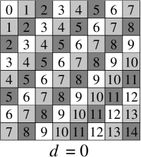
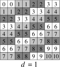
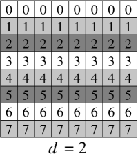
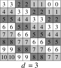
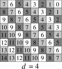
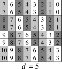
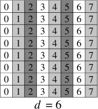
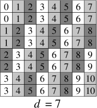
Fig. 1: Line number $k$ for pixels following direction $d=0:7$ in an $8\times 8$ block.

For each direction $d$, the pixel average for line $k$ is

$$\mu_{d,k}=\frac{1}{N_{d,k}}\sum_{p\in P_{d,k}}x_{p}\ ,$$ (1)

where $x_{p}$ is the value of pixel $p$, $P_{d,k}$ is the set of pixels in line $k$ following direction $d$ and $N_{d,k}$ is the cardinality of $P_{d,k}$ (for example, in Fig. 1, $N_{1,0}=2$ and $N_{1,4}=8$). The SSD is then

$$E_{d}^{2}=\sum_{k}\left[\sum_{p\in P_{d,k}}\left(x_{p}-\mu_{d,k}\right)^{2}\right]\ .$$ (2)

Substituting (1) into (2) and simplifying results in

$$E_{d}^{2}=\sum_{p}x_{p}^{2}-\sum_{k}\frac{1}{N_{d,k}}\left(\sum_{p\in P_{d,k}}x_{p}\right)^{2}\ .$$ (3)

Note that the simplifications leading to (3) are the same as to those allowing a variance to be computed as $\sigma_{x}^{2}=\frac{\sum x^{2}}{N}-\frac{\left(\sum x\right)^{2}}{N^{2}}$. Considering that the first term of (3) is constant with respect to $d$, we find the optimal direction $d_{opt}$ by maximizing the second term:

$$d_{opt} =\max_{d}s_{d}$$ (4)

$$s_{d} =\sum_{k}\frac{1}{N_{d,k}}\left(\sum_{p\in P_{d,k}}x_{p}\right)^{2}\ .$$ (5)

We can avoid the division in (5) by multiplying $s_{d}$ by 840, the least common multiple of the possible $N_{d,k}$ values ($1\leq N_{d,k}\leq 8$). When using 8-bit pixel data, and centering the values such that $-128\leq x_{p}\leq 127$, then $840s_{d}$ and all calculations needed for $s_{d}$ fit in a 32-bit signed integer. For higher bit depths, we downscale the pixels to $8$ bits during the direction search.

Fig. 2 shows an example of a direction search for an $8\times 8$ block containing a line. The step-by-step process is described in algorithm 1. To save on decoder complexity, we assume that luma and chroma directions are correlated, and only search the luma component. The same direction is used for the chroma components.

In total, the search for all 8 directions requires the following arithmetic operations:

1. The pixel accumulations in equation (5) can be implemented with 294 additions (reusing partial sums of adjacent pixels).

2. The accumulations result in 90 line sums. Each is squared, requiring 90 multiplies.

3. The $s_{d}$ values can be computed from the squared line sums with 34 multiplies and 82 additions.

4. Finding the largest $s_{d}$ value requires 7 comparisons.

The total is 376 additions, 124 multiplies and 7 comparisons. That is about two thirds of the number of operations required for the 8x8 IDCT in HEVC [5]. The code can be efficiently vectorized, with a small penalty due to the diagonal alignment, resulting in a complexity similar to that of an 8x8 IDCT.

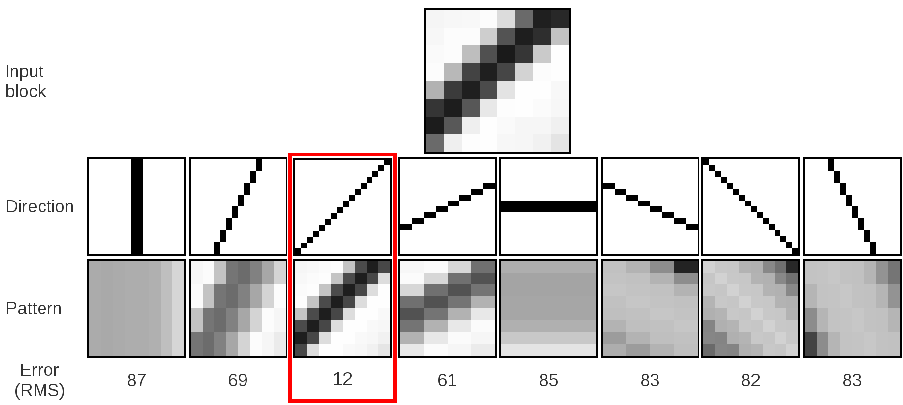
Fig. 2: Example of direction search for an $8\times 8$ block. The patterns shown are based on the $\mu_{d,k}$ values. In this case, the 45-degree direction is selected because it minimizes $E_{d}^{2}$. The error values $E_{d}$ shown are never computed in practice (only $s_{d}$ is).

  Initialize all variables to zero   for $d=0$ to $7$ do      for $i=0$ to $7$ do          for $j=0$ to $7$ do             $L\leftarrow\mathrm{line\_table}[d][i][j]$             $\mathrm{partial}[d][L]\leftarrow\mathrm{partial}[d][L]+\left(\mathrm{pixel}[i][j]-128\right)$             $\mathrm{count}[d][L]\leftarrow\mathrm{count}[d][L]+1$          end for      end for      for $L=0$ to $14$ do          if $\mathrm{count}[d][L]>0$ then             $s[d]\leftarrow s[d]+\mathrm{partial}[d][L]^{2}\cdot 840/\mathrm{count}[d][L]$          end if      end for   end for   for $d=0$ to $7$ do      if $s[d]>s[\mathrm{best\_}d]$ then          $\mathrm{best\_}d\leftarrow d$      end if   end for   $\mathrm{direction}\leftarrow\mathrm{best\_}d$   $\mathrm{directional\_contrast}\leftarrow s[\mathrm{best\_}d]-s[(\mathrm{best\_}d+4)\mod 8]$

Algorithm 1: Direction search. The line_table[$d$][$i$][$j$] values are the line numbers shown in Fig. 1. The $840/\mathrm{count}[d][L]$ terms can be pre-computed. More functionally equivalent algebraic simplifications are possible, but they are not shown here for clarity.

3 Non-linear Low-pass Filter

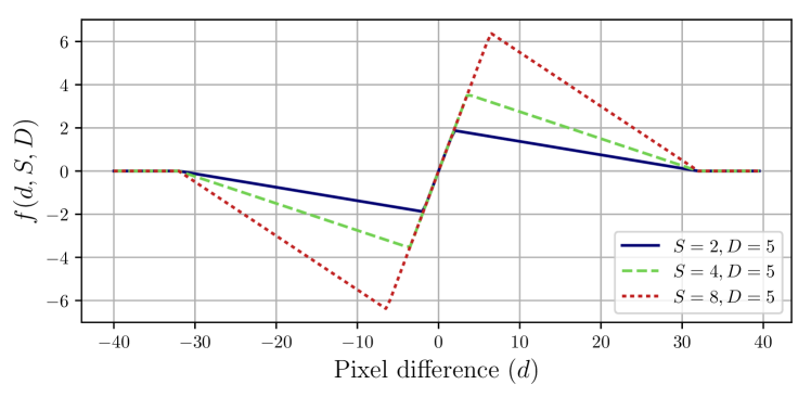
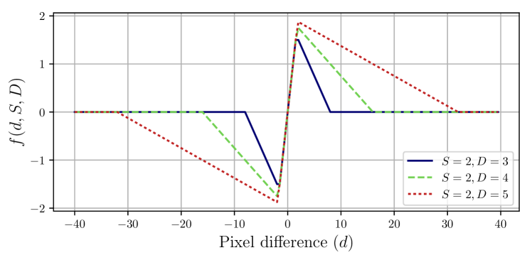
Fig. 3: Effect of strength (top) and damping (bottom) on $f(d,S,D)$.

CDEF uses a non-linear low-pass filter designed to remove coding artifacts without blurring sharp edges. It achieves this by selecting filter tap locations based on the identified direction, but also by preventing excessive blurring when the filter is applied across an edge. The latter is achieved through the use of a non-linear low-pass filter that deemphasizes pixels that differ too much from the pixel being filtered [6]. In one dimension, the non-linear filter is expressed as

$$y\left(i\right)=x\left(i\right)+\!\!\sum_{m}w_{k}f\left(x\left(i+m)-x(i\right),S,D\right)\ ,$$ (6)

where $w_{k}$ are the filter weights and $f(d,S,D)$ is a constraint function operating on the difference between the filtered pixel and each of the neighboring pixels. For small differences, $f\left(d,S,D\right)=d$, making the filter in (6) behave like a linear filter. When the difference is large, $f\left(d,S,D\right)=0$, which effectively ignores the filter tap. The filter is parametrized by a strength $S$ and a damping $D$:

$$f\left(d,S,D\right)=\left\{\begin{array}[]{ll}\!\!\min\left(d,\max\left(0,S-\left\lfloor{\frac{d}{2^{D-\lfloor{\log_{2}S}\rfloor}}}\right\rfloor\right)\right),d\geq 0\\ \!\!\max\left(d,\min\left(0,\left\lceil{\frac{-d}{2^{D-\lfloor{\log_{2}S}\rfloor}}}\right\rceil-S\right)\right),d<0\end{array}\right.$$ (7)

with $D\geq\lfloor\log_{2}{S}\rfloor$. The strength $S$ controls the maximum difference allowed and the damping $D$ controls the point where $f\left(d,S,D\right)=0$. Fig. 3 illustrates the effect of the strength and damping on $f(\cdot)$. The function is anti-symmetric around $d=0$.

3.1 Directional filter

The main reason for identifying the direction of the Section 2 is to align the filter taps along that direction to reduce ringing while preserving the directional edges or patterns. However, directional filtering alone sometimes cannot sufficiently reduce ringing. We also want to use filter taps on pixels that do not lie along the main direction. To reduce the risk of blurring, these extra taps are treated more conservatively. For this reason, CDEF defines primary taps and secondary taps. The primary taps follow the direction $d$, and the weights are shown in Fig. 4. For the primary taps, the weights alternate for every other strength, so that the weights for strengths 1, 3, 5, etc. are different from the weights for strengths 2, 4, 6, etc. The secondary taps form a cross, oriented $45^{\circ}$ off the direction $d$ and their weights are shown in Fig. 5. The complete 2-D CDEF filter is expressed as

$$y\left(i,j\right)= x(i,j)+\mathrm{round}\bigg{(}$$

$$\sum_{m,n}{w}^{(p)}_{d,m,n}f\left(x\left(m,n)-x(i,j\right),S^{(p)},D\right)$$

$$+ \sum_{m,n}{w}^{(s)}_{d,m,n}f\left(x\left(m,n)-x(i,j\right),S^{(s)},D\right)\bigg{)}\ ,$$ (8)

where $S^{(p)}$ and $S^{(s)}$ and the strengths of the primary and secondary taps, respectively, and $\mathrm{round}(\cdot)$ rounds ties away from zero.

Since the sum of all the primary and secondary weights exceed unity, it is possible (though rare) for the output $y(i,j)$ to change by more than the maximum difference between the input and the neighboring values. This is avoided by explicitly clamping the filter output based on the neighboring pixels with non-zero weights:

$$y_{clip}(i,j) =\min\left(y_{max},\max\left(y_{min},y(i,j)\right)\right)$$ (9)

$$y_{min} =\min_{m,n\in R}(x(i+m,j+n))$$ (10)

$$y_{max} =\max_{m,n\in R}(x(i+m,j+n))$$ (11)

$$R =(n,m)|{w}^{(p)}_{d,m,n}+{w}^{(s)}_{d,m,n}\neq 0$$ (12)

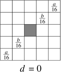
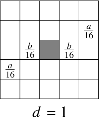
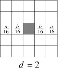
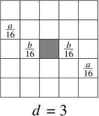
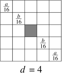
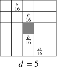
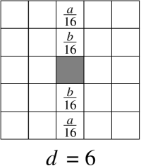
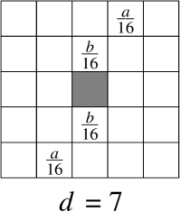
Fig. 4: Primary filter taps following direction $d=0:7$. For even strengths $a=2$ and $b=4$, whereas for odd strengths $a=3$ and $b=3$. The filtered pixel in shown in gray.

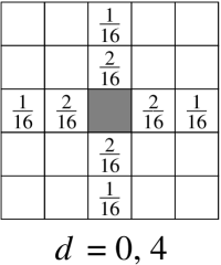
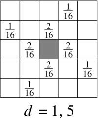
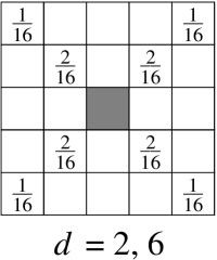
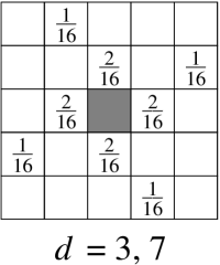
Fig. 5: Secondary filter taps following direction $d=0:7$. The filtered pixel is shown in gray.

The direction, strength and damping parameters are constant over each $8\times 8$ block being filtered. When processing the pixel at position $(i,j)$, the filter is allowed to use pixels $x(i+m,j+m)$ lying outside of the $8\times 8$ block. If the input pixel lies outside of the frame (visible area), then the pixel is ignored ($f(d,S,D)=0$). To maximize parallelism, CDEF always operates on the input (post-deblocking) pixels $x(i,j)$ so filtered pixels are never reused for filtering other pixels.

3.2 Valid strengths and damping values

The strengths $S^{(p)}$ and $S^{(s)}$ and damping $D$ must be set high enough to smooth out coding artifacts, but low enough to avoid blurring details in the image. For 8-bit content $S^{(p)}$ ranges between $0$ and $15$, and $S^{(s)}$ can be $0$, $1$, $2$ or $4$. $D$ ranges from $3$ to $6$ for luma, and the damping value for chroma is always one less. $D$ shall never be lower than the $\log_{2}S$ to ensure that the exponent of $2^{D-\lfloor{\log_{2}S}\rfloor}$ in (7) never becomes negative. For instance, if for chroma $S^{(p)}=15$ and the luma damping is $3$, the chroma damping shall also be $3$ (and not 2) because $\left\lfloor\log_{2}S^{(p)}\right\rfloor=3$.

For bit depths greater than 8 bits, $S^{(p)}$ and $S^{(s)}$ are scaled according to the extra bit depth, and $D$ is offset accordingly. For example, 12-bit content can have $S^{(p)}$ values of $0$, $16$, $32$, $...$, $240$, and $D$ ranges from $7$ to $10$. The strengths are scaled up after selecting the primary filter taps, so the taps still alternate, even though the scaling makes all values of $S^{(p)}$ even. Picking the optimal damping value is less critical than picking the optimal strengths. $S^{(p)}$ and $S^{(s)}$ are chosen independently for luma and chroma.

The signaled luma primary strength $S^{(p)}$ is adjusted for each $8\times 8$ block using the directional_contrast value ($v$) computed in algorithm 1:

$$S^{(p)}_{adj}=\left\{\begin{array}[]{ll}\left\lfloor\frac{S^{(p)}\left(4+\min\left(\left\lfloor\log_{2}\left\lfloor\frac{v}{2^{16}}\right\rfloor\right\rfloor,12\right)\right)+8}{16}\right\rfloor&,v\geq 2^{10}\\ 0&,\mathrm{otherwise}\end{array}\right.$$ (13)

The adjustment makes the filtering adapt to the amount of directional contrast and requires no signaling.

4 Signaling and Filter Blocks

The frame is divided into filter blocks of $64\times 64$ pixels. Some CDEF parameters are signaled at the frame level, and some may be signaled at the filter block level. The following is signaled at the frame level: the damping $D$ (2 bit), the number of bits used for filter block signaling (0-3, 2 bits), and a list of 1, 2, 4 or 8 presets. One preset contains the luma and chroma primary strengths (4 bits each), the luma and chroma secondary strengths (2 bits each), as well as the luma and chroma skip condition bits, for a total of 14 bits per preset. For each filter block, 0 to 3 bits are used to indicate which preset is used. The filter parameters are only coded for filter blocks that have some coded residual. Such “skipped” filter blocks have CDEF disabled. In filter blocks that do have some coded residual, any $8\times 8$ block with no coded residual also has filtering disabled unless the skip condition bit is set in that filter block’s preset.

Since the skip condition flag would be redundant in the case when both the primary and secondary filter strengths are $0$, this combination has a special meaning. In that case, the block shall be filtered with a primary filter strength equal to $19$, a secondary filter strength equal to $7$, and the skip condition still set.

When the chroma subsampling differs horizontally and vertically, e.g., for 4:2:2 video, the filter is disabled for chroma, and the chroma primary strength, the chroma skip condition flag and the chroma secondary strength are not signaled.

5 Encoder Search

Table 1: CDEF Bjøntegaard-delta [7] rate for the objective-1-fast test set in AWCY. The AV1 and Thor encoders were tested for a high-latency (HL) configuration, a real-time, low-latency (LL) configuration, as well as for low latency and low-complexity (LL+LC).

Encoding	PSNR	CIEDE	PSNR-HVS	SSIM	MS-SSIM
AV1 HL	-1.08%	-2.11%	-0.15%	-1.11%	-0.44%
AV1 LL	-1.93%	-2.88%	-0.86%	-1.96%	-1.18%
AV1 LL + LC	-3.68%	-4.54%	-2.50%	-4.15%	-3.05%
Thor HL	-2.26%	-3.13%	-0.49%	-2.75%	-1.39%
Thor LL	-3.19%	-5.18%	-1.34%	-3.31%	-2.23%
Thor LL + LC	-6.17%	-10.33%	-4.13%	-7.60%	-6.11%

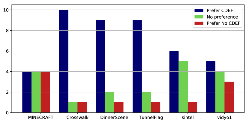
Fig. 6: Subjective A-B comparison results (with ties) for CDEF vs. no processing for the high-latency configuration.

On the encoder side, the search needs to determine both the frame level parameters (preset parameters, number of presets) and the filter block-level preset ID. Assuming the presets are already chosen, the ID for each non-skipped filter block is chosen by minimizing a distortion metric over the filter block. The simplest error metric is the sum of squared error (SSE), defined as $D=\left\|\mathbf{s}-\mathbf{d}\right\|^{2}$, where $\mathbf{s}$ is a vector containing the source (uncoded) pixels for the filter block and $\mathbf{d}$ contains the decoded pixels, filtered using a particular preset. While SSE leads to good results overall, it sometimes causes excessive smoothing in non-directional textured areas (e.g. grass). Instead, we use a modified version of SSE that takes into account contrast in a similar way to the structural similarity (SSIM) metric [8]. The distortion metric is the sum over the filter block of the following $8\times 8$ distortion function:

$$D_{8\times 8}=\frac{\sigma_{s}^{2}+\sigma_{d}^{2}+C_{1}}{2\sqrt{\sigma_{s}^{2}\sigma_{d}^{2}+C_{2}}}\cdot\left\|\mathbf{s}-\mathbf{d}\right\|^{2}\ ,$$ (14)

where $\sigma_{s}^{2}$ and $\sigma_{d}^{2}$ are the variances of $\mathbf{s}$ and $\mathbf{d}$ over the block and the constants are set to $C_{1}=6.25$ and $C_{2}=312.5$ for 8-bit depth. Using (14) degrades PSNR results, but improves visual quality. Since the distortion metric is only used in the encoder, it is not normative.

There are many possible strategies for choosing the presets for the frame, depending on the acceptable complexity requirements and whether the encoder is allowed to make two passes through the frame. In the two-pass case, the first step is to measure the distortion $D_{b,p}$ for each filter block b, for each combination $p$ of $S^{(p)}$, $S^{(s)}$ and skip condition bit ($16\times 4\times 2=128$ parameter combinations) and for each plane. Once the distortion values are computed, the goal is to find the two sets of presets $P_{\mathrm{luma}}$ and $P_{\mathrm{chroma}}$ that minimize the rate-distortion cost

$$J=\lambda B\log_{2}N+\sum_{b}\left(\min_{p\in P_{\mathrm{luma}}}D^{\mathrm{luma}}_{b,p}+\min_{p\in P_{\mathrm{chroma}}}D^{\mathrm{chroma}}_{b,p}\right)\ ,$$ (15)

where $N$ is the cardinality of $P_{\mathrm{luma}}$ and $P_{\mathrm{chroma}}$ and $B$ is the number of filter blocks. While we are not aware of polynomial-time algorithms to find the global minimum, we have found that a greedy search can produce near-optimal results. With the greedy search, we start by finding the optimal presets for $N=1$ and then increment $N$ by finding the optimal preset to add while keeping the already-selected presets $1..N-1$ constant. If the encoder can afford the complexity, it is possible to improve on the purely greedy search by iteratively re-optimizing one preset at a time.

The high complexity version of the search described above typically results in less than 1% of the encoding time. Still, for low complexity operation, it is possible to reduce the search complexity by only considering a subset of the 128 possible presets. This results in only a small loss ($<0.1\%$ BD-rate) in quality.

The damping value may be determined from the quantizer alone, with larger damping values used for larger quantizers.

6 Results

We tested CDEF with the Are We Compressed Yet [9] online testing tool using the AV1 and Thor [10, 11] codecs, both still in development at the time of writing. BD-rate results for PSNR, PSNR-HVS [12], CIEDE2000 [13], SSIM [8], and MS-SSIM [14] are shown in Table 1 for the objective-1-fast test set. These results reflect the gains in the codebases for git SHA’s e200b28 [15] (8^th August 2017) and b5e5cc5 [16] (21^st October 2017) for AV1 and Thor respectively.

Subjective tests conducted on AV1 for the high-latency configuration show a statistically significant ($p<.05$) improvement for 3 out of 6 clips, as shown in Fig. 6. Considering that it usually takes in the order of 5% improvement in BD-rate to obtain such statistically significant results, and the tested configuration is the one with the smallest BD-rate improvement, we believe the visual improvement is higher than the BD-rate results suggest.

The objective results show that CDEF performs better when encoding with fewer tools and simpler search algorithms. In some sense, CDEF “competes” for the same gains as some other coding tools. Considering that CDEF is significantly less complex to encode than many of the AV1 tools, it provides a good way of reducing the complexity of an encoder. In terms of decoder complexity, CDEF represents between 3% and 10% of the AV1 decoder (depending on the configuration).

7 Conclusion

We have demonstrated CDEF, an effective in-loop filtering algorithm for removing coding artifacts in the AV1 and Thor video codecs. The filter is able to effectively remove artifacts without causing blurring through a combination of direction-adaptive filtering and a non-linear filter with signaled parameters. Objective results show a bit-rate reductions up to 4.5% on AV1 and 10.3% on Thor. These results are confirmed by subjective testing.

CDEF should be applicable to other video codecs as well as image codecs. In the case of AV1, an open questions that remains is how to optimally combine its search with that of “Loop Restoration” [17], another in-loop enhancement filter in AV1.

8 Acknowledgments

We thank Thomas Daede for organizing the subjective test.

References

- [1] G. J. Sullivan, J. Ohm, W.-J. Han, and T. Wiegand, “Overview of the high efficiency video coding (HEVC) standard,” IEEE Transactions on circuits and systems for video technology, vol. 22, no. 12, pp. 1649–1668, 2012.
- [2] C. M. Fu, E. Alshina, A. Alshin, Y. W. Huang, C. Y. Chen, C. Y. Tsai, C. W. Hsu, S. M. Lei, J. H. Park, and W. J. Han, “Sample adaptive offset in the HEVC standard,” IEEE Transactions on Circuits and Systems for Video Technology, vol. 22, no. 12, pp. 1755–1764, Dec 2012.
- [3] C. Tomasi and R. Manduchi, “Bilateral filtering for gray and color images,” in Proceedings of IEEE International Conference on Computer Vision, 1998.
- [4] T. J. Daede, N. E. Egge, J.-M. Valin, G. Martres, and T. B. Terriberry, “Daala: A perceptually-driven next generation video codec,” in Proceedings Data Compression Conference (DCC), 2016.
- [5] M. Budagavi, A. Fulseth, and G. Bjøntegaard, “HEVC transform and quantizaion,” in High Efficiency Video Coding (HEVC). Springer, 2014, pp. 162–166.
- [6] S. Midtskogen, A. Fuldseth, G. Bjøntegaard, and T. Davies, “Integrating Thor tools into the emerging AV1 codec,” in Proceedings International Conference on Image Processing (ICIP), 2017.
- [7] T. Daede and J. Moffitt, “Video codec testing and quality measurement,” https://tools.ietf.org/html/draft-daede-netvc-testing, 2015.
- [8] Z. Wang, A. C. Bovik, H. R. Sheikh, and E. P. Simoncelli, “Image quality assessment: from error visibility to structural similarity,” IEEE Transactions on image processing, vol. 13, no. 4, pp. 600–612, 2004.
- [9] “AreWeCompressedYet?” https://arewecompressedyet.com/.
- [10] G. Bjøntegaard, T. Davies, A. Fuldseth, and S. Midtskogen, “The Thor video codec,” in Proceedings Data Compression Conference (DCC), 2016.
- [11] T. Davies, G. Bjøntegaard, A. Fuldseth, and S. Midtskogen, “Recent improvements to Thor with emphasis on perceptual coding tools,” proc. SPIE 9971, Applications of Digital Image Processing XXXIX, September 2016.
- [12] N. Ponomarenko, F. Silvestri, K.Egiazarian, M. Carli, and V. Lukin, “On between-coefficient contrast masking of dct basis functions,” in Proceedings of Third International Workshop on Video Processing and Quality Metrics for Consumer Electronics VPQM-07, 2007.
- [13] M. R. Luo, G. Cui, and B. Rigg, “The development of the cie 2000 colour-difference formula: Ciede2000,” Color Research & Application, vol. 26, no. 5, pp. 340–350, 2001.
- [14] Z. Wang, E. P. Simoncelli, and A. C. Bovik, “Multiscale structural similarity for image quality assessment,” in Signals, Systems and Computers, 2004. Conference Record of the Thirty-Seventh Asilomar Conference on, vol. 2. IEEE, 2003, pp. 1398–1402.
- [15] “AV1 source code repository,” https://aomedia.googlesource.com/aom.
- [16] “Thor source code repository,” https://github.com/cisco/thor.
- [17] D. Mukherjee, S. Li, Y. Chen, A. Anis, S. Parker, and J. Bankoski, “A switchable loop-restoration with side-information framework for the emerging AV1 video codec,” in Proceedings International Conference on Image Processing (ICIP), 2017.