Thermal quantum metrology in memoryless and correlated environments

Abstract

In bosonic quantum metrology, the estimate of a loss parameter is typically performed by means of pure states, such as coherent, squeezed or entangled states, while mixed thermal probes are discarded for their inferior performance. Here we show that thermal sources with suitable correlations can be engineered in such a way to approach, or even surpass, the error scaling of coherent states in the presence of general Gaussian decoherence. Our findings pave the way for practical quantum metrology with thermal sources in optical instruments (e.g., photometers) or at different wavelengths (e.g., far infrared, microwave or X-ray) where the generation of quantum features, such as coherence, squeezing or entanglement, may be extremely challenging.

I Introduction

Quantum metrology SamMETRO ; Caves ; Paris ; Giova ; ReviewMETRO ; ReviewNEW is one of the most active research areas in quantum information science NiCh ; Hayashi ; Watrous . The possibility to exploit quantum resources to boost the estimation of unknown parameters encoded in quantum states or channels is appealing for a variety of practical tasks, from gravitational wave detection grav1 ; grav2 to frequency standards freq and clock synchronization clock1 ; clock2 . In the specific framework of continuous-variable systems WeeRMP ; SamRMP , parameter estimation typically involves the statistical inference of the phase Parisbounds ; OlivaresSpe ; Paris07 ; GenoniParis ; GenoniParis2 ; Dowling2 ; Dowling3 ; GenoniKim ; Raf0 ; Escher ; Yue ; Raf1 ; Raf2 ; Bagan or loss MonrasParis ; Treps ; Venzel ; AdessoIlluminati ; Gaiba ; MonrasIlluminati accumulated by a bosonic mode propagating through a Gaussian channel. For this task, Gaussian and non-Gaussian resources have been extensively studied ReviewNEW .

While the minimization of the estimation error over all quantum strategies is crucial to show the ultimate precision achievable by quantum mechanics, it is also important to study practical applications to realistic scenarios, where the access to quantum resources may be limited and the presence of decoherence may even destroy the quantum advantage shown for the noiseless models. This is an important gap to fill for bosonic systems, where previous studies on loss estimation were devoted to finding the optimal error scaling reachable by squeezing, entanglement or other highly non-classical features in decoherence-free scenarios MonrasParis ; Treps ; Venzel ; Gaiba .

Here we extend the state-of-the-art on bosonic loss estimation in two ways. First of all, we consider the practical use of correlated-thermal sources which can be easily engineered by using a beam splitter. These sources are generally designed to be asymmetric so that only a few mean photons are irradiated through the unknown lossy channel, while the majority of them are deviated onto an ancillary channel. Thanks to this asymmetric splitting, the lossy channel is ‘non-invasively’ probed with low energy, while enough correlations are created with the ancillary photons to improve the final detection.

This practical scheme is relevant in various realistic scenarios. For instance, this is the simplest strategy to improve the optical setups of photometers and spectrophotometers currently employed in experimental biology. These instruments use thermal lamps at optical or UV wavelengths to measure the concentration of bacteria, cells, or nucleic acids (DNA/RNA) in fragile biological samples via an estimation of the transmissivity Ingle . Our interferometric design would introduce correlations and greatly improve their performance.

Other important scenarios are the far infrared and microwave regimes where quantum features are hard to generate. By contrast, correlated-thermal sources can be easily generated in these cases, and could be adopted (in the long run) to advance applications such as protein Terahertz spectroscopy or magnetic resonance imaging. Similar implications could also be envisaged at very high-frequencies, where quasi-monochromatic X-ray beams can now be generated by small-scale all-laser-driven Compton sources with good spatial-temporal coherence Powers . These thermal beams could be manipulated by X-ray beam splitters based on Laue-Bragg diffraction Oberta or other X-ray interferometry Nugent .

Besides the focus on cheap correlated-thermal sources, the second novelty of our work is to provide the first study of loss estimation assuming a general model of Gaussian decoherence, which includes additional loss, thermal effects and even the possibility of environmental correlations. Thanks to this general model, we can potentially account for many effects, including detector inefficiencies, thermal background (which is non-trivial at the microwave regime) and also the presence of non-Markovian dynamics in the environment.

In such a general scenario, we fix the benchmark to be the performance of coherent states: The generation of minimum uncertainty states can be regarded as the minimal requirement for a single-mode source to be considered ‘quantum’. While the direct use of single-mode thermal sources is clearly sub-optimal, we show that the coherent-state benchmark can easily be achieved by two-mode thermal sources which are asymmetric and correlated. Surprisingly, these sources are even able to largely outperform the coherent-state benchmark when (separable) correlations are present in the environment.

II Quantum Metrology with Correlated-Thermal Sources

Let us start with a detailed description of the correlated-thermal source (see also Fig. 1). We consider two single-mode thermal states, $\rho_{H}$ and $\rho_{L}$, with mean numbers of photons equal to $\bar{n}_{H}$ and $\bar{n}_{L}$, respectively. These are chosen to satisfy $\bar{n}_{H}>\bar{n}_{L}$ and we may specifically consider $\bar{n}_{L}=0$. The two thermal states are combined with a generally unbalanced beam splitter, with transmissivity $\eta\leq 1/2$. The three parameters of the source ($\eta$, $\bar{n}_{H}$ and $\bar{n}_{L}$) are chosen in such a way that the mean number of photons transmitted on mode $A$, equal to $\bar{n}=\eta\bar{n}_{H}+(1-\eta)\bar{n}_{L}$, is fixed to some low value (e.g., $\bar{n}=10$), while no energetic constraint is imposed for mode $B$.

As mentioned above, the most interesting situation is when the source is highly asymmetric. This means that we take $\bar{n}_{H}\gg\bar{n}_{L}\simeq 0$ and $\eta\ll 1$, in such a way that $\bar{n}\simeq\eta\bar{n}_{H}$ is kept small, while mode $B$ is very energetic with $\simeq\bar{n}_{H}$ photons transmitted. Locally, the reduced state $\rho_{A}$ ($\rho_{B}$) is a faint (bright) thermal state, but globally the state $\rho_{AB}$ is highly correlated. One can check that the quadrature operators associated with the two modes ($\hat{q}_{A}$,$\hat{p}_{A}$, $\hat{q}_{B}$ and $\hat{p}_{B}$) have covariances $\left\langle\hat{q}_{A}\hat{q}_{B}\right\rangle=\left\langle\hat{p}_{A}\hat{p}_{B}\right\rangle\simeq-\bar{n}\eta^{-1/2}$, whose absolute value is $\gg 1$.

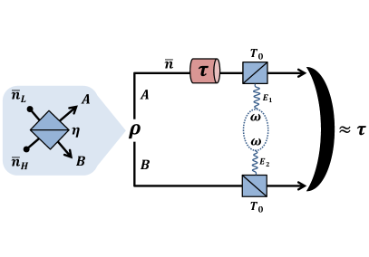
Figure 1: Bosonic loss estimation with correlated-thermal sources under general Gaussian decoherence. On the left we show the preparation of a two-mode thermal source $\rho_{AB}$ which is correlated and generally asymmetric. This is prepared using a beam splitter with transmissivity $\eta\leq 1/2$, which mixes a bright thermal state (with photon number $\bar{n}_{H}$) with a faint thermal state (with photon number $\bar{n}_{L}<$ $\bar{n}_{H}$). The three parameters of the source ($\eta$, $\bar{n}_{H}$ and $\bar{n}_{L}$) are chosen in such a way that the mean number of photons $\bar{n}$ on mode $A$ is fixed to some low value, while the energy of mode $B$ is not constrained. On the right, the input thermal source and an optimal output measurement are employed for estimating the unknown transmissivity $\tau$ of the red box (lossy channel). This is done in the presence of Gaussian decoherence, modelled by two beam splitters with transmissivity $T_{0}$ and injecting thermal noise with variance $\omega$. The environmental thermal modes $E_{1}$ and $E_{2}$ may be uncorrelated or correlated.

The generated thermal source $\rho_{AB}(\eta,\bar{n}_{H},\bar{n}_{L})$ is then used to probe a lossy channel $\mathcal{E}_{\tau}$ with unknown transmissivity $\tau\in[0,1]$ on mode $A$. In a realistic scenario, this is affected by decoherence, here modelled by a generally-joint Gaussian channel $\mathcal{D}$ affecting both modes $A$ and $B$. This can be represented by two beam splitters with transmissivity $T_{0}$ mixing $A$ and $B$ with ancillary modes, $E_{1}$ and $E_{2}$, coming from the environment. These ancillas inject thermal noise $\omega=\bar{n}_{\text{env}}+1/2$, where $\bar{n}_{\text{env}}$ is the mean number of photons of the bath. Furthermore, the two environmental ancillas may also be correlated, which means that their quadrature operators, i.e., $\hat{q}_{E_{1}}$,$\hat{p}_{E_{1}}$, $\hat{q}_{E_{2}}$ and $\hat{p}_{E_{2}}$, have non-zero covariance, i.e., $\left\langle\hat{q}_{E_{1}}\hat{q}_{E_{2}}\right\rangle=g$ and $\left\langle\hat{p}_{E_{1}}\hat{p}_{E_{2}}\right\rangle=g^{\prime}$, satisfying suitable constraints CMbona ; CMbona2 (see Appendix C). Thus, the output Gaussian state is given by $\rho_{AB}^{\text{out}}(\tau)=\mathcal{D}\circ(\mathcal{E}_{\tau}\otimes\mathcal{I})(\rho_{AB})$.

At the output a joint quantum measurement $\mathcal{M}$ is performed on modes $A$ and $B$ whose outcome provides an estimate of $\tau$. In the basic formulation of quantum metrology, this process is assumed to be performed many times, so that a large number $N\gg 1$ of input states $\rho_{AB}^{\otimes N}$ are prepared and their outputs $\rho_{AB}^{\text{out}}(\tau)^{\otimes N}$ are subject to a collective quantum measurement $\mathcal{M}^{\otimes N}$, whose output is classically processed into an unbiased estimator $\tilde{\tau}_{N}$ of $\tau$. For large $N$, the resulting error-variance $\sigma^{2}(\tau,N):=\langle(\tilde{\tau}_{N}-\tau)^{2}\rangle$ satisfies the quantum Cramer-Rao (QCR) bound $\sigma^{2}(\tau,N)\geq\left[NH(\tau)\right]^{-1}$, where $H(\tau)$ is the quantum Fisher information (QFI) SamMETRO . The QFI can be expressed as $H(\tau)=8(1-F)/d\tau^{2}$, where $F$ is the quantum fidelity between the two Gaussian states $\rho_{AB}^{\text{out}}(\tau)$ and $\rho_{AB}^{\text{out}}(\tau+d\tau)$, which can be computed using the general formula of Ref. Benki . It is important to note that the QCR bound can always be achieved, asymptotically, by an optimal measurement $\mathcal{M}^{\otimes N}~{}$SamMETRO .

In the following we show the performances achievable by our correlated-thermal sources under various assumptions for the Gaussian decoherence model, starting from the simple case of a pure-loss environment, to including thermal noise and, finally, noise-correlations. These performances are compared with the use of a single-mode thermal source and, most importantly, with a coherent-state benchmark. The latter can easily be evaluated. Considering the scenario at the right of Fig. 1, but neglecting mode $B$ and considering an input coherent state $\left|\alpha\right\rangle$ with $\left|\alpha\right|^{2}=\bar{n}$ on mode $A$, we derive the benchmark (see Appendix B for details)

$$H_{\text{coh}}(\tau)=\frac{\gamma_{\text{dec}}\bar{n}}{\tau},~{}~{}~{}~{}\gamma_{\text{dec}}:=\frac{T_{0}}{T_{0}+2(1-T_{0})\omega}.$$ (1)

In this formula, we can see how the error-scaling $\varpropto\bar{n}/\tau$ is moderated by the factor $\gamma_{\text{dec}}$ taking into account of the Gaussian decoherence.

III Pure-loss decoherence

Let us start with the simplest decoherence model, which only considers additional damping on top of the unknown lossy channel under estimation. In other words, we consider the two beam splitters with $T_{0}<1$ in a zero temperature bath ($\omega=1/2$) and without noise correlations ($g=g^{\prime}=0$). This is the most typical situation at the optical regime, where thermal background is negligible. Such a pure-loss decoherence may be found in many scenarios. For instance, it may be the effect of detector inefficiencies, beam spreading, or the use of fiber components. In other cases, it may due to the typical configuration of an optical instrument. For example, in a photometer, the measure of a concentration within a sample (via its optical transmission) is typically performed with respect to a blank sample whose intrinsic transmissivity is known and fixed.

Let us estimate the transmissivity parameter $\tau$ by constraining the mean number of photons in the signal mode $A$, e.g., $\bar{n}=10$, and assuming additional (known) loss in modes $A$ and $B$, e.g., quantified by $T_{0}=0.7$. We then construct correlated-thermal sources combining a strongly attenuated thermal state $\bar{n}_{L}=10^{-4}\simeq 0$ (approximately the vacuum state) and a thermal state with $\bar{n}_{H}=\bar{n}\eta^{-1}$, where the parameter $\eta$ of the beam splitter is variable and completely describes the source. The corresponding QFI $H_{\eta}(\tau)$ is plotted in Fig. 2, where the performances of these sources are compared with that of the single-mode thermal state (achievable by setting $\eta=1$) and that of the coherent state probes, according to Eq. (1) with $\gamma_{\text{dec}}=T_{0}$.

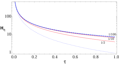
Figure 2: Quantum Fisher information $H_{\eta}$ versus transmissivity $\tau$ for probes irradiating $\bar{n}=10$ signal photons. We plot the performances of the correlated-thermal source for $\eta=1/2$, $1/10$ and $1/100$ (solid red lines); larger $H_{\eta}$ indicates better precision. These are compared with the single-mode thermal state (dotted blue line) and the coherent-state benchmark (dashed blue line, which coincides with the solid red line for $\eta=1/100$). Here we consider $T_{0}=0.7$, $\omega=1/2$ (zero temperature bath), and $g=g^{\prime}=0$ (corresponding to no correlations in the environment).

As we can see from Fig. 2, the correlated-thermal source is optimal in the most asymmetric configurations, where the beam splitter is highly unbalanced (e.g., $\eta=1/100$) so that strong correlations are generated between the signal mode $A$ and the ancillary mode $B$, while keeping the signal energy low at $\bar{n}=10$ photons. The coherent-state benchmark is easily approached already with reasonable asymmetries (e.g., $\eta=1/10$). It is remarkable that the performance achievable by coherent photons on mode $A$ can also be achieved by employing an equivalent number of thermal photons (as long as they are suitably correlated with the ancillary mode $B$).

Note that highly-asymmetric beam splitters are typical in X-ray interferometry. A hard X-ray beam at $25~{}$KeV (suitable for medical applications, such as mammography) can be split by Silicon crystals via Laue–Bragg diffraction. For crystals of sufficient depth $\simeq 200~{}\mu$m, the diffraction efficiency (reflectivity of the beam splitter) can reach values of $1/100$ Oberta .

IV Thermal-loss decoherence

We now include the presence of thermal noise in the decoherence process. Besides various technical imperfections (e.g., stray photons emitted by the source), this noise may come from a natural thermal background which is non-negligible at far infrared and microwave wavelengths. As an example, consider the frequency of $3.5$ THz. At room temperature ($300$ K) there will be $\bar{n}_{\text{env}}\simeq 1.33$ mean thermal photons entering the interferometric setup (via the input ports $E_{1}$ and $E_{2}$ of the two beam splitters of Fig. 1). Assuming a liquid-nitrogen temperature ($77$ K) for the preparation beam splitter, we have $\bar{n}_{L}\simeq 0.12$. We then consider high loss ($T_{0}=0.4$) and signals with $\bar{n}=20$ photons. As we can see from Fig. 3, correlated-thermal sources with enough asymmetry are again able to approach the coherent-state benchmark.

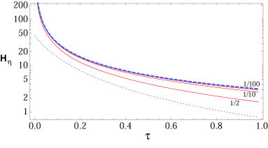
Figure 3: Quantum Fisher information $H_{\eta}$ versus transmissivity $\tau$ for probes irradiating $\bar{n}=20$ signal photons. We plot the performances of the correlated-thermal source with $\bar{n}_{L}\simeq 0.12$ and having $\eta=1/2$, $1/10$ and $1/100$ (solid red lines); larger $H_{\eta}$ indicates better precision. These are compared with the single-mode thermal state (dotted blue line) and the coherent-state benchmark (dashed blue line). Here we consider $T_{0}=0.4$, $\omega\simeq 1.33+1/2$ (room temperature at $3.5$ THz), and $g=g^{\prime}=0$ (corresponding to no correlations in the environment).

V Correlated-noise decoherence

We finally consider noise correlations in the Gaussian environment. There may be situations, e.g., on a small scale, where two bosonic modes experience exactly the same fluctuations. In these ‘non-Markovian’ environments, we find that our correlated-thermal sources can even beat the coherent-state benchmark. More specifically, we consider noise-correlations of the type $g=g^{\prime}=1/2-\omega\leq 0$, which are maximal but still separable (i.e., the state of the environmental ancillas $E_{1}$ and $E_{2}$ is not entangled). These specific environmental correlations constructively combine with those of the input two-mode thermal source in a way as to reduce the net effect of decoherence.

Consider $T_{0}=0.8$ and $\bar{n}_{\text{env}}\simeq 20.34$ (e.g., corresponding to $300$ GHz at room temperature). We shall assume we have correlated-thermal sources with $\bar{n}_{L}\simeq 8.3\times 10^{-3}$ (e.g., via a cryogenic preparation), variable $\eta$, and irradiating $\bar{n}=50$ photons on mode $A$. As we can see from Fig. 4, all choices of sources beat the coherent-state benchmark. In particular, the best solution is the fully-symmetric thermal source with $\eta=1/2$, which is the most effective at counterbalancing the specific symmetric noise of the environment. We can easily extend this analysis to considering an environment with asymmetric thermal noise, in which case the best performance is achieved by asymmetric thermal sources. This is shown in Appendix D, where we also check that the coherent benchmark is not beaten if the environmental correlations are of the “positive type” $g=g^{\prime}>0$, therefore not sustaining those “negative” $\left\langle\hat{q}_{A}\hat{q}_{B}\right\rangle=\left\langle\hat{p}_{A}\hat{p}_{B}\right\rangle<0$ of the input correlated state.

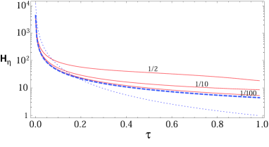
Figure 4: Quantum Fisher information $H_{\eta}$ versus transmissivity $\tau$ for probes irradiating $\bar{n}=50$ signal photons. We plot the performances of the correlated-thermal source with $\bar{n}_{L}\simeq 8.3\times 10^{-3}$ and having $\eta=1/2$, $1/10$ and $1/100$ (solid red lines); larger $H_{\eta}$ indicates better precision. These are compared with the single-mode thermal state (dotted blue line) and the coherent-state benchmark (dashed blue line). Here $T_{0}=0.8$, $\omega\simeq 20.34+1/2$ and $g=g^{\prime}=1/2-\omega$.

VI Conclusions

We have shown that thermal sources can be engineered in such a way that their correlations may non-trivially improve the performance of loss estimation in practical setups of quantum metrology considering various scenarios of Gaussian decoherence. Correlated-thermal sources with strong energetic asymmetry are able to approach the performance of coherent state probes in Markovian (memoryless) models of Gaussian decoherence, where the bosonic modes are affected by independent and identical noise fluctuations. In the presence of correlated noise in the environment, as typical of non-Markovian dynamics, we have shown that the correlated-thermal sources can even beat the coherent state benchmark, a feature which may be achieved by correctly combining the types of correlations created in the source with those present in the environment.

According to our investigations, the behavior represented in the previous numerical examples is generic as long as the mean number of photons on mode $A$ is reasonably low, and the preparation of the correlated-thermal source involves a faint thermal state with sufficiently low thermal number $\bar{n}_{L}$ (ideally, this should be the vacuum state). One may argue that the correlations employed in our sources still have a quantum component, e.g., as quantified by quantum discord DiscordRMP (which is exactly computable for these types of Gaussian states OptimalityDiscord ). In this respect, we notice that discord may be considered as the cheapest non-classical feature to be generated in a bipartite source. Indeed, in our case, it just corresponds to the ability of combining thermal states at a beam splitter, which just requires sufficient spatial-temporal coherence in the bosonic modes. Clearly, this is much less demanding than the ability to generate minimum uncertainty states or even squeezing.

Further work includes the analysis of loss estimation with a finite number of signals, and the design of explicit detection strategies able to approach the theoretical performance of the quantum Cramer-Rao bound. For the case of a pure-loss environment ($\omega=1/2$), we provide this study in Appendix E, where we show that photon-counting applied to a correlated-thermal source achieve the same energy scaling in $\bar{n}$ of the coherent-state benchmark (but with a different pre-factor).

Another potential investigation is considering adaptive strategies for loss estimation, whose optimal perfomance is unknown. A possible methodology to exploit is that of channel simulation recently developed in quantum metrology ReviewMETRO ; PirCo ; PBTstretch after successful applications in quantum and private communications PLOB ; TQC . It would also be very interesting to analyze the explicit performance of correlated-thermal sources for practical tasks of quantum hypothesis testing QHT ; QHT1 ; QHT2 ; UNA1 ; UNA2 ; UNA3 ; UNA4 ; UNA5 ; Invernizzi , such as the quantum reading of optical memories Qread ; Qread2 ; Qread3 ; Qread4 ; Qread4b ; Qread5 ; Qread6 ; Qread7 ; Qread7b ; Qread7c ; Qread8 ; Qread9 ; Qread9b ; Qread10 and the quantum illumination of targets Qill0 ; Qill1 ; Qill1b ; Qill2 ; Qill3 ; Qillexp1 ; Qillexp2 ; Qillexp3 .

Appendix A Relations with previous literature

Previous literature on quantum metrology with bosonic systems has been devoted to the estimation of various parameters of a Gaussian channel, including displacement, phase-shift, loss and thermal parameters. Optimal estimation of displacements was studied in Ref. GenoniJoint . Phase estimation has undergone an extensive analysis: Bounds on the precision of phase-estimation using Gaussian resources were studied in Ref. Parisbounds ; optimized interferometry for phase estimation was given in Ref. OlivaresSpe ; and the use of squeezing in high-sensitive interferometry was analyzed in Refs. Paris07 ; Dowling2 ; Dowling3 . Phase estimation was also extended to the presence of decoherence, mainly phase diffusion and photon loss. For instance, it was extended to phase diffusion in Refs. GenoniParis ; GenoniParis2 , to unitary and random linear disturbance in Ref. GenoniKim , and to lossy optical interferometry in Refs. Raf0 ; Escher ; Yue , with associated general studies of quantum metrology with uncorrelated noise Raf1 ; Raf2 . Phase estimation with displaced thermal states and squeezed thermal state was studied in Ref. Bagan  also considering the presence of loss.

There is relatively less literature regarding the estimation of the loss parameter. Optimal estimation of loss in Gaussian channels was studied in Ref. MonrasParis by using single-mode pure Gaussian states (see also Ref. Treps ). This analysis was also carried out for entangled Gaussian states in Ref. Venzel and non-Gaussian sources in Ref. AdessoIlluminati . All these studies were performed in the absence of decoherence. Use of squeezing for estimating the interaction parameter in bilinear bosonic Hamiltonians (including beam-splitter interactions) was also discussed in Ref. Gaiba . Later, Ref. MonrasIlluminati considered the joint estimation of damping and temperature of a Gaussian channel by means of Gaussian states, specifically showing the superior performances achieved by the use of entanglement over coherent states. Note that this study considered the presence of thermal noise directly in the single-mode Gaussian channel under estimation, not the presence of a lossy and thermal environment (affecting signal and ancillary modes) on top of the channel to be estimated. Finally, the detection of loss by using squeezed thermal states (in absence of decoherence) was analyzed in the framework of quantum hypothesis testing Invernizzi .

Our work departs from all this previous literature in several aspects. First of all, it is clearly not related with the extensive literature on phase estimation, since we are considering the loss parameter. Then, with respect to previous works on bosonic damping estimation, we are:

(i) Engineering new correlated-type of thermal states, void of squeezing, and never investigated before for quantum metrology tasks. These cheap sources are important for making quantum metrology practical, especially when considering longer wavelengths, where quantum features are challenging to generate.

(ii) Considering a general model of Gaussian decoherence affecting both signal and ancillary modes, which may introduce loss, thermal noise, and even two-mode correlations. It is important to note that this type of decoherence is added on top of the lossy channel to be estimated, and may describe various realistic scenarios, such as the detector inefficiencies, thermal background (e.g., at the microwaves), and potential non-Markovian effects.

Appendix B Coherent-state benchmark

First of all, a brief remark on the notation. We consider quadrature operators $\hat{q}$ and $\hat{p}$ with canonical commutation relations $[\hat{q},\hat{p}]=i$, so that the annihilation operator corresponds to $\hat{a}=(\hat{q}+i\hat{p})/\sqrt{2}$ and the vacuum shot-noise is equal to $1/2$. Correspondingly, the covariance matrix (CM) of a single-mode thermal state is equal to $\mu\mathbf{I}$, where $\mu=\bar{n}+1/2$, with $\bar{n}$ being the mean number of thermal photons. For the general formalism of continuous-variable systems and Gaussian states, the reader may consult the reviews of Refs. WeeRMP ; SamRMP .

Let us prepare mode $A$ in a coherent state $\left|\alpha\right\rangle$ with $\bar{n}=\left|\alpha\right|^{2}$ mean photons. This state has mean value $\mathbf{\bar{x}}=(\bar{q},\bar{p})^{T}$ where $\alpha=(\bar{q}+i\bar{p})/\sqrt{2}$ and covariance matrix (CM) equal to $\mathbf{I}/2$. This is subject to the action of the lossy channel $\mathcal{E}_{\tau}$ followed by that of the thermal-loss decoherence channel $\mathcal{D}_{A}$ with transmissivity $T_{0}$ and thermal noise $\omega$. At the output, the two statistical moments of $\rho_{\alpha}(\tau,T_{0},\omega)=(\mathcal{D}_{A}\circ\mathcal{E}_{\tau})(\left|\alpha\right\rangle\left\langle\alpha\right|)$ are given by $\mathbf{\bar{x}}^{\prime}=\sqrt{T_{0}\tau}\mathbf{\bar{x}}$ and $\mathbf{V}^{\prime}=a^{\prime}\mathbf{I}$, where

$$a^{\prime}:=\frac{T_{0}}{2}+(1-T_{0})\omega~{}.$$ (2)

To derive the QFI, we first compute the fidelity between $\rho_{1}:=\rho_{\alpha}(\tau,T_{0},\omega)$ and $\rho_{2}:=\rho_{\alpha}(\tau+d\tau,T_{0},\omega)$. These two states have the same CM $V_{1}=V_{2}=a^{\prime}\mathbf{I}$, and their mean values differ by $\delta=\sqrt{T_{0}}(\sqrt{\tau+d\tau}-\sqrt{\tau})\mathbf{\bar{x}}$. Using the formula of Ref. Benki , it is straightforward to compute their fidelity

$$F(\rho_{1},\rho_{2}) =\exp\left[-\frac{1}{4}\delta^{T}(V_{1}+V_{2})^{-1}\delta\right]$$ (3)

$$=\exp\left[-\frac{T_{0}}{4a^{\prime}}(\sqrt{\tau+d\tau}-\sqrt{\tau})^{2}\bar{n}\right].$$ (4)

Using the latter expression in

$$H(\tau)=\frac{8\left[1-F(\rho_{1},\rho_{2})\right]}{d\tau^{2}}~{},$$ (5)

and expanding in $d\tau$, we derive the following expression of the quantum Fisher information (QFI)

$$H(\tau)=\frac{T_{0}}{T_{0}+2(1-T_{0})\omega}\frac{\bar{n}}{\tau}+O(d\tau)~{}.$$ (6)

Appendix C Correlated-thermal sources

C.1 Characterization

First of all, let us construct the correlated-thermal source. We start from two single-mode thermal states, $\rho_{H}$ and $\rho_{L}$, with mean number of photons equal to $\bar{n}_{H}$ and $\bar{n}_{L}$, respectively (with $\bar{n}_{H}>\bar{n}_{L}$). These states have zero mean and CMs

$$\mathbf{V}_{H}=\mu_{H}\mathbf{I},~{}~{}~{}\mathbf{V}_{L}=\mu_{L}\mathbf{I},$$ (7)

where $\mu_{H(L)}=\bar{n}_{H(L)}+1/2$. These states are taken as input of a beam-splitter of transmissivity $\eta$. At the output modes, $A$ and $B$, we have a Gaussian state with zero mean and CM

$$\mathbf{V}_{AB}=\left(\begin{array}[c]{cc}a\mathbf{I}&c\mathbf{I}\\ c\mathbf{I}&b\mathbf{I}\end{array}\right),$$ (8)

where

$$a :=\eta\mu_{H}+(1-\eta)\mu_{L}~{},b:=\eta\mu_{L}+(1-\eta)\mu_{H}~{},$$ (9)

$$c :=\sqrt{\eta(1-\eta)}(\mu_{L}-\mu_{H})\text{~{}}.$$ (10)

In our study we fix $\bar{n}=a-1/2=\eta\bar{n}_{H}+(1-\eta)\bar{n}_{L}$ to some low value, and we change $\eta$ to create the desired asymmetry between modes $A$ and $B$.

Note that the correlations are of the negative type $c<0$. Their (unrestricted) quantum discord can be easily quantified, since it coincides with their Gaussian discord, according to the results of Ref. OptimalityDiscord .

C.2 Evolution

This correlated-thermal source is sent to probe the lossy channel $\mathcal{E}_{\tau}$ in the presence of general Gaussian decoherence $\mathcal{D}$. To model the latter, let us assume a more general scenario than that of Fig. 1, where the two ancillary modes $E_{1}$ and $E_{2}$ may have different thermal noise, $\omega_{1}$ and $\omega_{2}$. In other words, we consider an environment described by a Gaussian state with general CM

$$\mathbf{V}_{E_{1}E_{2}}=\left(\begin{array}[c]{cc}\omega_{1}\mathbf{I}&\mathbf{G}\\ \mathbf{G}&\omega_{2}\mathbf{I}\end{array}\right),~{}~{}\mathbf{G}=\left(\begin{array}[c]{cc}g&\\ &g^{\prime}\end{array}\right).$$ (11)

In order to be a physical state, this CM must satisfy a set of constraints, given by CMbona ; CMbona2

$$\left|g\right|<\sqrt{\omega_{1}\omega_{2}},~{}~{}\left|g^{\prime}\right|<\sqrt{\omega_{1}\omega_{2}},~{}~{}\nu^{2}\geq\frac{1}{4}$$ (12)

where

$$\nu^{2}:=\frac{\Delta-\sqrt{\Delta^{2}-4\det\mathbf{V}_{E_{1}E_{2}}}}{2},~{}~{}\Delta=\omega_{1}^{2}+\omega_{2}^{2}+2gg^{\prime}~{}.$$ (13)

Then, we have a separable state if we also impose $\tilde{\nu}^{2}\geq 1/4$, where

$$\tilde{\nu}^{2}:=\frac{\tilde{\Delta}-\sqrt{\tilde{\Delta}^{2}-4\det\mathbf{V}_{E_{1}E_{2}}}}{2},~{}~{}\tilde{\Delta}=\omega_{1}^{2}+\omega_{2}^{2}-2gg^{\prime}~{}.$$ (14)

We find that, in the specific case where $g=g^{\prime}$, the condition

$$\left|g\right|=\frac{\sqrt{(2\omega_{1}-1)(2\omega_{2}-1)}}{2}$$ (15)

guarantees that the state is both physical and separable.

After the action of the lossy channel and the Gaussian environment, the output Gaussian state $\rho_{AB}^{\text{out}}(\tau)=\mathcal{D}\circ(\mathcal{E}_{\tau}\otimes\mathcal{I})(\rho_{AB})$ has zero mean and CM

$$\mathbf{V}_{AB}^{\text{out}}(\tau)=\left(\begin{array}[c]{cccc}\tilde{a}&&c_{1}&\\ &\tilde{a}&&c_{2}\\ c_{1}&&\tilde{b}&\\ &c_{2}&&\tilde{b}\end{array}\right),$$ (16)

where

$$\tilde{a} :=T_{0}\tau a+\frac{T_{0}(1-\tau)}{2}+(1-T_{0})\omega_{1},$$ (17)

$$\tilde{b} :=T_{0}b+(1-T_{0})\omega_{2},$$ (18)

$$c_{1} :=T_{0}\sqrt{\tau}c+(1-T_{0})g,~{}c_{2}:=T_{0}\sqrt{\tau}c+(1-T_{0})g^{\prime}\text{~{}}.$$ (19)

C.3 Numerical computation of the quantum Fisher information

To derive the QFI, we first compute the quantum fidelity between the two (zero-mean) Gaussian states $\rho_{AB}^{\text{out}}(\tau)$ and $\rho_{AB}^{\text{out}}(\tau+d\tau)$. Following the notation of Ref. Benki , we re-arrange the CM (16) according the ordering $\hat{q}_{A},\hat{q}_{B},\hat{p}_{A}$ and $\hat{p}_{B}$, so that

$$\mathbf{V}_{AB}^{\text{out}}(\tau)=\left(\begin{array}[c]{cc}\tilde{a}&c_{1}\\ c_{1}&\tilde{b}\end{array}\right)\oplus\left(\begin{array}[c]{cc}\tilde{a}&c_{2}\\ c_{2}&\tilde{b}\end{array}\right).$$ (20)

Setting $\mathbf{V}_{1}=\mathbf{V}_{AB}^{\text{out}}(\tau)$ and $\mathbf{V}_{2}=\mathbf{V}_{AB}^{\text{out}}(\tau+d\tau)$, we compute the auxiliary matrix

$$\mathbf{V}_{\text{aux}}=\boldsymbol{\Omega}^{T}(\mathbf{V}_{1}+\mathbf{V}_{2})^{-1}\left(\frac{\boldsymbol{\Omega}}{4}+\mathbf{V}_{2}\boldsymbol{\Omega}\mathbf{V}_{1}\right),$$

where $\boldsymbol{\Omega}:=\begin{pmatrix}0&\mathbf{I}\\ -\mathbf{I}&0\end{pmatrix}$ is the symplectic form. Finally, the quantum fidelity is given by Benki

$$F(\tau)=\sqrt[4]{\frac{\det\left[2\left(\sqrt{\mathbf{I}+\frac{1}{4}(\mathbf{V}_{\text{aux}}\boldsymbol{\Omega})^{-2}}+\mathbf{I}\right)\mathbf{V}_{\text{aux}}\right]}{\det(\mathbf{V}_{1}+\mathbf{V}_{2})}}.$$

The latter expression can be expanded for small $d\tau$ and replaced in the following formula for the QFI

$$H(\tau)=\frac{8\left[1-F(\tau)\right]}{d\tau^{2}}~{}.$$ (21)

With this approach we can numerically derive the curves shown in the figures of the main text.

Appendix D Asymmetrically-correlated environment

For the sake of completeness, we consider here an example where the environment is correlated but its ancillas introduce different values of thermal noise. The scenario coincides with that of Fig. 1 of the main text, but now we allow for a more general Gaussian state for the environment, where the modes $E_{1}$ and $E_{2}$ have thermal noise $\omega_{1}$ and $\omega_{2}$, respectively. We then assume that the environmental state is separable with correlations of the type

$$g=g^{\prime}=\frac{-\sqrt{(2\omega_{1}-1)(2\omega_{2}-1)}}{2}~{}.$$ (22)

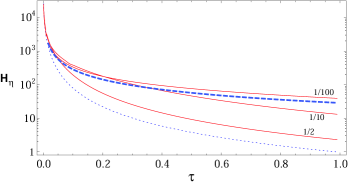
Figure 5: Quantum Fisher information $H_{\eta}$ versus transmissivity $\tau$ for probes irradiating $\bar{n}=50$ signal photons. We plot the performances of the correlated-thermal source with $\bar{n}_{L}\simeq 8.3\times 10^{-3}$ and having $\eta=1/2$, $1/10$ and $1/100$ (solid red lines); larger $H_{\eta}$ indicates better precision. These are compared with the single-mode thermal state (dotted blue line) and the coherent-state benchmark (dashed blue line). Here we consider $T_{0}=0.8$, $\omega_{1}=1+1/2$, $\omega_{2}=100+1/2$, and $g=g^{\prime}<0$ as in Eq. (22).

From Fig. 5 we see that, for strongly asymmetric noise $\omega_{2}\gg\omega_{1}$, the coherent-state benchmark can only be beaten by a sufficiently asymmetric thermal source ($\eta=1/100$), which sends the majority of the photons through the noisier channel. It is important to remark that the classical benchmark is outperformed because the “negative type” of correlations in the environment ($g=g^{\prime}<0$) tend to sustain the “negative type” of correlations in the input thermal source ($c<0$). If the environment has the “positive type” of correlations ($g=g^{\prime}>0$), then there is a destructive effect and the classical benchmark is not beaten. See Fig. 6.

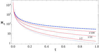
Figure 6: Quantum Fisher information $H_{\eta}$ versus transmissivity $\tau$ for probes irradiating $\bar{n}=50$ signal photons. As in Fig. 5 but taking positive correlations $g=g^{\prime}=\sqrt{(2\omega_{1}-1)(2\omega_{2}-1)}/2$.

Appendix E Practical receiver designs

Here we consider explicit receiver designs based on photon counting, homodyne and heterodyne detection. We obtain analytical solutions for $\bar{n}_{L}=0$, $\omega_{1}=\omega_{2}=1/2$, and $g=g^{\prime}=0$, in which case the CM in Eq. (16) reads

$$\mathbf{V}_{AB}^{\mathrm{out}}(\tau)=\left(\begin{array}[c]{cc}\frac{1}{2}+\tau\eta n_{H}^{\prime}\mathbf{I}&-n_{H}^{\prime}\sqrt{\tau\eta(1-\eta)}\mathbf{I}\\ -n_{H}^{\prime}\sqrt{\tau\eta(1-\eta)}\mathbf{I}&\frac{1}{2}+(1-\eta)n_{H}^{\prime}\mathbf{I}\end{array}\right)\,,$$ (23)

and we have defined $n_{H}^{\prime}:=T_{0}\bar{n}_{H}$.

Photon-counting. The symplectic eigenvalues of the CM in Eq. (23) are $\frac{1}{2}$ and $\frac{1}{2}+(1+\tau\eta-\eta)n_{H}^{\prime}$. This means that the state $\rho_{AB}^{\mathrm{out}}(\tau)$ can be written as tensor product, $\rho_{AB}^{\mathrm{out}}(\tau)=\rho_{A^{\prime}}^{\mathrm{out}}\otimes\rho_{B^{\prime}}^{\mathrm{out}}(\tau)$, where $\rho_{A^{\prime}}^{\mathrm{out}}$ is the vacuum state of the mode $A^{\prime}$ and $\rho_{B^{\prime}}^{\mathrm{out}}(\tau)$ is a thermal state of the mode $B^{\prime}$ with $m=(1+\tau\eta-\eta)n_{H}^{\prime}$ mean photons. Denote as $A,A^{{\dagger}}$ and $B,B^{{\dagger}}$ the canonical creation and annihilation operators of the original pair of modes, and denote as $A^{\prime},{A^{\prime}}^{{\dagger}}$ and $B^{\prime},{B^{\prime}}^{{\dagger}}$ those of the new pair of modes. One can easily check that

$$A^{\prime}=(\sin{\theta)}\,A-(\cos{\theta)}\,B,~{}B^{\prime}=(\cos{\theta)}\,A+(\sin{\theta)}\,B,$$ (24)

with

$$\cos{\theta}=-\sqrt{\frac{\tau\eta}{1+\tau\eta-\eta}},~{}\sin{\theta}=\sqrt{\frac{1-\eta}{1+\tau\eta-\eta}}.$$ (25)

Therefore, the state $\rho_{B^{\prime}}^{\mathrm{out}}(\tau)$ can be written as

$$\rho_{AB}^{\mathrm{out}}(\tau)=\frac{1}{1+m}\sum_{k=0}^{\infty}\left(\frac{m}{1+m}\right)^{k}|\psi_{k}\rangle\langle\psi_{k}|,$$ (26)

where $\psi_{k}$ is the state with $k$ photons in the mode $B^{\prime}$, i.e.,

$$|\psi_{k}\rangle =\frac{1}{\sqrt{k!}}\left(\cos{\theta}\,A^{{\dagger}}+\sin{\theta}\,B^{{\dagger}}\right)^{k}|0\rangle$$ (27)

$$=\frac{1}{\sqrt{k!}}\sum_{j=0}^{k}{\binom{k}{j}}\left(\cos{\theta}\,A^{{\dagger}}\right)^{j}\left(\sin{\theta}\,B^{{\dagger}}\right)^{k-j}|0\rangle$$ (28)

$$=\frac{1}{\sqrt{k!}}\sum_{j=0}^{k}{\binom{k}{j}}\sqrt{j!(k-j)!}\left(\cos{\theta}\right)^{j}\left(\sin{\theta}\right)^{k-j}|j,k-j\rangle$$ (29)

$$=\sum_{j=0}^{k}\sqrt{{\binom{k}{j}}}\left(\cos{\theta}\right)^{j}\left(\sin{\theta}\right)^{k-j}|j,k-j\rangle\,.$$ (30)

From the expression in Eq. (26) we can easily compute the joint probability of measuring $N_{A}$ and $N_{B}$ photons, which is

$$P(N_{A},N_{B})$$

$$=\frac{1}{1+m}\left(\frac{m}{1+m}\right)^{N_{A}+N_{B}}{\binom{N_{A}+N_{B}}{N_{A}}}\left(\cos{\theta}\right)^{2N_{A}}\left(\sin{\theta}\right)^{2N_{B}}$$ (31)

$$=\frac{1}{1+m}\left(\frac{n_{H}^{\prime}}{1+m}\right)^{N_{A}+N_{B}}{\binom{N_{A}+N_{B}}{N_{A}}}\left(\tau\eta\right)^{N_{A}}\left(1-\eta\right)^{N_{B}}\,.$$ (32)

To compute the (classical) Fisher information associated to this measurement (photon-counting) we first compute the logarithmic derivative of $P(N_{A},N_{B})$ with respect to $\tau$, getting

$$\frac{\partial\log{P(N_{A},N_{B})}}{\partial\tau}$$

$$=\frac{1}{\tau}\frac{N_{A}[1+(1-\eta)n_{H}^{\prime}]-(1+N_{B})\tau\eta n_{H}^{\prime}}{1+n_{H}^{\prime}(1+\tau\eta-\eta)}$$ (33)

and then we derive the Fisher information

$$\mathrm{FI} =\langle\left[\frac{\partial\log{P(N_{A},N_{B})}}{\partial\tau}\right]^{2}\rangle$$ (34)

$$=\frac{1+(1-\eta)n_{H}^{\prime}}{1+(1+\tau\eta-\eta)n_{H}^{\prime}}\,\frac{\eta n_{H}^{\prime}}{\tau}\,.$$ (35)

In terms of $\bar{n}=\eta n_{H}=\eta\bar{n}_{H}=\eta n_{H}^{\prime}/T_{0}$ we obtain the scaling

$$\mathrm{FI}=\frac{\gamma_{\text{phc}}\bar{n}}{\tau},~{}\gamma_{\text{phc}}:=\frac{T_{0}+(1-\eta)T_{0}^{2}\bar{n}\eta^{-1}}{1+(1+\tau\eta-\eta)T_{0}\bar{n}\eta^{-1}}.$$ (36)

Therefore, we recover the same behaviour (up to a small correction) of the coherent-state benchmark (ideally this benchmark is achieved in the limit $\eta\rightarrow 0$ with $n$ kept constant).

Homodyne and heterodyne detection. Consider, for example, that the $q$ quadratures of the two modes $A$ and $B$ are detected. The outcomes of the measurements are two correlated Gaussian variables $q_{A}$, $q_{B}$ with joint probability density $G(q_{A},q_{B})$ with CM

$$V_{q}=\left(\begin{array}[c]{cc}\frac{1}{2}+\tau\eta n_{H}^{\prime}&-n_{H}^{\prime}\sqrt{\tau\eta(1-\eta)}\\ -n_{H}^{\prime}\sqrt{\tau\eta(1-\eta)}&\frac{1}{2}+(1-\eta)n_{H}^{\prime}\end{array}\right).$$ (37)

The (classical) Fisher information of these correlated Gaussian variables reads:

$$\mathrm{FI}=\int dq_{A}dq_{B}G(q_{A},q_{B})\left[\frac{\partial\log{G(q_{A},q_{B})}}{\partial\tau}\right]^{2}.$$ (38)

Instead of computing this integral directly, we can exploit unitary invariance and work in the modes $A^{\prime}$, $B^{\prime}$ in which the state becomes a direct product and the CM is diagonal with eigenvalues $\frac{1}{2}$ and $\frac{1}{2}+(1+\tau\eta-\eta)n_{H}^{\prime}$. We then obtain

$$\mathrm{FI} =\int dq_{B}G(q_{B})\left[\frac{\partial\log{G(q_{B})}}{\partial\tau}\right]^{2}$$ (39)

$$=\frac{1}{2}\left[\frac{\eta n_{H}^{\prime}}{\frac{1}{2}+(1+\tau\eta-\eta)n_{H}^{\prime}}\right]^{2}$$ (40)

Similarly, for heterodyne detection we obtain the following expression for the CM:

$$\mathrm{FI}=\left[\frac{\eta n_{H}^{\prime}}{1+(1+\tau\eta-\eta)n_{H}^{\prime}}\right]^{2}\,.$$ (41)

In conclusion, we notice that both homodyne and heterodyne detection are far from being optimal measurements.

References

- (1) S. L. Braunstein, and C. M. Caves, Phys. Rev. Lett. 72, 3439 (1994).
- (2) C. M. Caves, and G. J. Milburn, Ann. Phys. 247, 135 (1996).
- (3) M. G. A. Paris, Int. J. Quant. Inf. 7, 125-137 (2009).
- (4) V. Giovannetti, S. Lloyd, and L. Maccone, Nature Photon. 5, 222 (2011).
- (5) R. Laurenza, C. Lupo, G. Spedalieri, S. L. Braunstein, and S. Pirandola, Quantum Meas. Quantum Metrol. 5, 1-12 (2018).
- (6) D. Braun et al., Preprint arXiv:1701.05152 (2017). In press on Reviews of Modern Physics.
- (7) J. Watrous, The theory of quantum information (Cambridge University Press, Cambridge, 2018). Also available from https://cs.uwaterloo.ca/~watrous/TQI/TQI.pdf
- (8) M. Hayashi, Quantum Information Theory: Mathematical Foundation (Springer-Verlag Berlin Heidelberg, 2017).
- (9) M. A. Nielsen, and I. L. Chuang, Quantum computation and quantum information (Cambridge University Press, Cambridge, 2000).
- (10) C. M. Caves, Phys. Rev. D 23, 1693 (1981).
- (11) K. Goda et al., Nature Phys. 4, 472 (2008).
- (12) S. F. Huelga et al., Phys. Rev. Lett. 79, 3865 (1997).
- (13) R. Jozsa, D. S. Abrams, J. P. Dowling, and C. P. Williams, Phys. Rev. Lett. 85, 2010 (2000).
- (14) M. de Burgh and S. D. Bartlett, Phys. Rev. A 72, 042301 (2005).
- (15) C. Weedbrook et al., Rev. Mod. Phys. 84, 621 (2012).
- (16) S. L. Braunstein and P. van Loock, Rev. Mod. Phys. 77, 513 (2005).
- (17) M. G. Genoni et al., Phys. Rev. A 87, 012107 (2013).
- (18) C. Sparaciari, S. Olivares, and M. G. A. Paris, J. Opt. Soc. Am. B 32, 1354-1359 (2015).
- (19) S. Olivares, and M. G. A. Paris, Optics and Spectroscopy 103, 231-236 (2007).
- (20) M. G. A. Paris, Physics Letters A 201, 132-138 (2007).
- (21) P. M. Anisimov et al., Phys. Rev. Lett. 104, 103602 (2010).
- (22) W. N. Plick, J. P. Dowling, and G. S. Agarwal, New J. Phys. 12, 083014 (2010).
- (23) M. G Genoni, S. Olivares, and M. G. A. Paris, Phys. Rev. Lett. 106, 153603 (2011).
- (24) M. G. Genoni et al., Phys. Rev. A 85, 043817 (2012).
- (25) D. D. de Souza, M. G. Genoni, and M. S. Kim, Phys. Rev. A 90, 042119 (2014).
- (26) R. Demkowicz-Dobrzański et al., Phys. Rev. A 80, 013825 (2009).
- (27) B. M. Escher, R. L. de Matos Filho, and L. Davidovich, Nat. Phys. 7, 406–411 (2011).
- (28) J.-D. Yue, Y.-R. Zhang, and H. Fan, Sci. Rep. 4, 5933 (2014).
- (29) R. Demkowicz-Dobrzański et al., Nature Commun. 3, 1063 (2012).
- (30) J. Kołodyński and R. Demkowicz-Dobrzański, New J. Phys. 15, 073043 (2013).
- (31) M. Aspachs, J. Calsamiglia, R. Munoz Tapia, and E. Bagan, Phys. Rev. A 79, 033834 (2009).
- (32) A. Monras, and M. G. A. Paris, Phys. Rev. Lett. 98, 160401 (2007).
- (33) O. Pinel, P. Jian, N. Treps, C. Fabre, and D. Braun, Phys. Rev. A 88, 040102 (2013).
- (34) H. Venzl and M. Freyberger, Phys. Rev. A 75, 042322 (2007).
- (35) G. Adesso, F. Dell’Anno, S. De Siena, F. Illuminati, and L. A. M. Souza, Phys. Rev. A 79, 040305(R) (2009).
- (36) R. Gaiba, and M. G. A. Paris, Phys. Lett. A 373, 934-939 (2009).
- (37) A. Monras, and F. Illuminati, Phys. Rev. A 83, 012315 (2011).
- (38) J. D. Ingle and S. R. Crouch, Spectrochemical Analysis (Prentice Hall, New Jersey, 1988).
- (39) N. D. Powers et al, Nat. Photon. 8, 28-31 (2014).
- (40) P. Oberta, and R. Mokso, Nuclear Instruments and Methods in Physics Research A 703, 59 (2013).
- (41) K. A. Nugent, Advances in Physics 59, 1-99 (2010).
- (42) S. Pirandola, A. Serafini, and S. Lloyd, Phys. Rev. A 79, 052327 (2009).
- (43) S. Pirandola, New J. Phys. 15, 113046 (2013).
- (44) L. Banchi, S. L. Braunstein, and S. Pirandola, Phys. Rev. Lett. 115, 260501 (2015).
- (45) K. Modi, A. Brodutch, H. Cable, T. Paterek, and V. Vedral, Rev. Mod. Phys. 84, 1655-1707 (2012).
- (46) S. Pirandola, G. Spedalieri, S. L. Braunstein, N. J. Cerf, and S. Lloyd, Phys. Rev. Lett. 113, 140405 (2014).
- (47) S. Pirandola, and C. Lupo, Phys. Rev. Lett. 118, 100502 (2017).
- (48) S. Pirandola, R. Laurenza, and C. Lupo, Fundamental limits to quantum channel discrimination, arXiv:1803.02834 (2018).
- (49) S. Pirandola, R. Laurenza, C. Ottaviani, and L. Banchi, Nat. Commun. 8, 15043 (2017). See also arXiv:1510.08863 (2015).
- (50) S. Pirandola, S. L. Braunstein, R. Laurenza, C. Ottaviani, T. P. W. Cope, G. Spedalieri, and L. Banchi, Quantum Sci. Technol. 3, 035009 (2018).
- (51) C. W. Helstrom, Quantum Detection and Estimation Theory (New York: Academic, 1976).
- (52) A. Chefles, Contemp. Phys. 41, 401 (2000).
- (53) S. M. Barnett and S. Croke, Adv. Opt. Photon. 1, 238-278 (2009).
- (54) J. A. Bergou, U. Herzog, and M. Hillery, Discrimination of Quantum States, in Quantum state estimation, Lecture Notes in Physics, Springer-Verlag Berlin Heidelberg (2004), pp 417-465.
- (55) Y. Sun, J. A. Bergou, and M. Hillery, Phys. Rev. A 66, 032315 (2002).
- (56) J. A. Bergou, and M. Hillery, Phys. Rev. Lett. 94, 160501 (2005).
- (57) J. A. Bergou, V. Bužek, E. Feldman, U. Herzog, and M. Hillery, Phys. Rev. A 73, 062334 (2006).
- (58) J. A. Bergou, E. Feldman, and M. Hillery, Phys. Rev. A 73, 032107 (2006).
- (59) C. Invernizzi, M. G.A. Paris, and S Pirandola, Phys. Rev. A 84, 022334 (2011).
- (60) S. Pirandola, Phys. Rev. Lett. 106, 090504 (2011).
- (61) S. Pirandola, C. Lupo, V. Giovannetti, S. Mancini, and S. L. Braunstein, New J. Phys. 13, 113012 (2011).
- (62) R. Nair, Phys. Rev. A 84, 032312 (2011).
- (63) O. Hirota, Quantum Meas. Quantum Metrol. 4, 70–73 (2017); See also arXiv:1108.4163 (2011).
- (64) S. Guha, Z. Dutton, R. Nair, J. H. Shapiro, and B. Yen, OSA Technical Digest, Optical Society of America), paper LTuF2 (2011).
- (65) A. Bisio, M. Dall’Arno, and G. M. D’Ariano, Phys. Rev. A 84, 012310 (2011).
- (66) M. Dall’Arno, A. Bisio, G. M. D’Ariano, M. Miková, M. Ježek, and M. Dušek, Phys. Rev. A 85, 012308 (2012).
- (67) G. Spedalieri, C. Lupo, S. Mancini, S. L. Braunstein, and S. Pirandola, Phys. Rev. A 86, 012315 (2012).
- (68) M. Dall’Arno, A. Bisio, and G. M. D’Ariano, Int. J. Quant. Inf. 10, 1241010 (2012).
- (69) S. Guha, and J. H. Shapiro, Phys. Rev. A 87, 062306 (2013).
- (70) C. Lupo, S. Pirandola, V. Giovannetti, and S. Mancini, Phys. Rev. A 87, 062310 (2013).
- (71) J. Prabhu Tej, A. R. Usha Devi, and A. K Rajagopal, Phys. Rev. A 87, 052308 (2013).
- (72) G. Spedalieri, Entropy 17, 2218-2227 (2015).
- (73) C. Lupo, and S. Pirandola, Quantum Inf. Comput. 17, 0611 (2017).
- (74) S. Lloyd, Science 321, 1463 (2008).
- (75) S.-H. Tan, B. I. Erkmen, V. Giovannetti, S. Guha, S. Lloyd, L. Maccone, S. Pirandola, and J. H. Shapiro, Phys. Rev. Lett. 101, 253601 (2008).
- (76) J. H. Shapiro, and S. Lloyd, New J. Phys. 11, 063045 (2009).
- (77) S. Barzanjeh, S. Guha, C. Weedbrook, D. Vitali, J. H. Shapiro, and S. Pirandola, Phys. Rev. Lett. 114, 080503 (2015).
- (78) C. Weedbrook, S. Pirandola, J. Thompson, V. Vedral, and M. Gu, New J. Phys. 18, 043027 (2016).
- (79) E. D. Lopaeva, I. Ruo Berchera, I. P. Degiovanni, S. Olivares, G. Brida, M. Genovese, Phys. Rev. Lett. 110, 153603 (2013).
- (80) Z. Zhang, M. Tengner, T. Zhong, F. N. C. Wong, and J. H. Shapiro, Phys. Rev. Lett. 111, 010501 (2013).
- (81) Z. Zhang, S. Mouradian, F. N. C. Wong, and J. H. Shapiro, Phys. Rev. Lett. 114, 10506 (2015).