A Simple Approach to the Supernova Progenitor-Explosion Connection

Abstract

We present a new approach to understand the landscape of supernova explosion energies, ejected nickel masses, and neutron star birth masses. In contrast to other recent parametric approaches, our model predicts the properties of neutrino-driven explosions based on the pre-collapse stellar structure without the need for hydrodynamic simulations. The model is based on physically motivated scaling laws and simple differential equations describing the shock propagation, the contraction of the neutron star, the neutrino emission, the heating conditions, and the explosion energetics. Using model parameters compatible with multi-D simulations and a fine grid of thousands of supernova progenitors, we obtain a variegated landscape of neutron star and black hole formation similar to other parameterised approaches and find good agreement with semi-empirical measures for the “explodability” of massive stars. Our predicted explosion properties largely conform to observed correlations between the nickel mass and explosion energy. Accounting for the coexistence of outflows and downflows during the explosion phase, we naturally obtain a positive correlation between explosion energy and ejecta mass. These correlations are relatively robust against parameter variations, but our results suggest that there is considerable leeway in parametric models to widen or narrow the mass ranges for black hole and neutron star formation and to scale explosion energies up or down. Our model is currently limited to an all-or-nothing treatment of fallback and there remain some minor discrepancies between model predictions and observational constraints.

1 Introduction

The connection between the properties of progenitors of core-collapse supernovae (SNe) and the properties of the resulting explosion and the compact remnant is one of the outstanding problems in stellar astrophysics. Systematically understanding this connection from first principles is difficult because the problem of the core-collapse supernova explosion mechanism has not yet been finally solved (see, e.g., Janka 2012; Burrows et al. 2012 for reviews). Supernova theory, however, now becomes testable due to observational findings and indirect constraints on the supernova explosion mechanism on three completely different fronts.

Over the recent years, direct observations of core-collapse supernova explosions based on large surveys and the combination of observations with archival data have yielded important insights about properties such as the minimum and maximum progenitor mass of Type II-P supernovae (Smartt et al., 2009; Smartt, 2009, 2015), the demography of progenitors of different supernova types in the HR diagram (see Smartt, 2009 for a review), and possible correlations, e.g., between explosion energy and nickel mass (Hamuy, 2003) and between progenitor mass and explosion energy (Poznanski, 2013; Chugai & Utrobin, 2014; Pejcha & Prieto, 2015).

The distribution of neutron star and black holes masses (Kiziltan et al., 2013; Özel et al., 2012, 2010), remnant kicks, and spins of young neutron stars (Faucher-Giguère & Kaspi, 2006; Ng & Romani, 2007; Repetto et al., 2012) provides additional constraints on the inner workings of the supernova engine and the progenitor–remnant connection (e.g., Schwab et al., 2010; Fryer et al., 2012; Pejcha & Thompson, 2012; Janka, 2013; Kochanek, 2015; Clausen et al., 2015).

The progenitor–explosion connection and the explosion mechanism are intimately linked with the nucleosynthetic contribution of core-collapse supernovae to the chemical evolution of galaxies. Supernova theory needs to account not only for the population-integrated yields of all massive stars (in the vein of Rauscher et al. 2002); it must also explain the non-uniformity of heavy-element nucleosynthesis channels emerging from stellar abundance studies (e.g., Travaglio et al., 2004; Ting et al., 2012; Hansen et al., 2012, 2014), which is thought to be related to the existence of core-collapse supernova sub-populations. More indirect constraints on the fate of massive stars come from, for example, the comparison of the observed star formation and supernova rates (Horiuchi et al., 2011; Botticella et al., 2012) and the limit for the diffuse supernova neutrino background (Beacom, 2010).

To interpret these observational findings and constraints and their implications for the core-collapse supernova explosion mechanism in a systematic and statistical way, we are still largely relegated to simplified analytic or parameterised numerical models, and this is also the approach we follow here. It is exceedingly difficult to connect first-principle simulations of core-collapse supernova explosions to the observable explosion properties and the remnant mass distribution for several reasons: Despite recent successes in 3D explosion modelling (Melson et al., 2015a; Melson et al., 2015b; Lentz et al., 2015; Müller, 2015), obtaining explosions has proved more difficult in 3D multi-group neutrino transport models than in 2D (Hanke et al., 2013; Tamborra et al., 2014; Takiwaki et al., 2014). Even in 2D, extending successful multi-group models to sufficiently late times to obtain saturated values for the explosion energy and remnant mass remains difficult (Müller et al., 2012a, b; Janka et al., 2012; Bruenn et al., 2013; Suwa et al., 2010; Summa et al., 2015; O’Connor & Couch, 2015), although the models of Bruenn et al. (2016) and Müller (2015) come close to this point. Even ignoring these obstacles, scanning the full parameter space of progenitor models in zero-age main sequence (ZAMS) mass, metallicity, and rotation rate with 3D simulations will remain impractical in the near future.

For this reason, approximate analytic models or parameterised simulations presently remain indispensable for understanding the connection between progenitor and explosion properties. Indeed, they are arguably becoming more useful as fully-fledged simulations provide an impetus and corrective for their improvement. Earlier studies (Fryer, 1999; Fryer & Kalogera, 2001; Heger et al., 2003) relied on a simple comparison of a parameterised explosion energy (obtained from a fit to – now outdated – 2D SPH simulations) to the binding energy of the envelope to predict the ultimate fate of the remnant (neutron star vs. black hole). Recent studies have taken some steps to improve this simple approach to various degrees in order to obtain a more consistent estimate of the time of shock revival, the “initial” explosion energy pumped into the ejecta during the first few seconds by the supernova engine, and the resulting fallback and residual accretion onto the compact remnant. Fryer et al. (2012) and Belczynski et al. (2012) used an analytic estimate of the internal energy in the gain region at the time of shock revival as a proxy for the explosion energy and then calculated the fallback numerically to obtain the remnant mass distribution, but their choice of the time of shock revival remains very much ad hoc. Pejcha & Thompson (2015) used analytic scaling laws for the critical neutrino luminosity required for shock revival and various contributions to the explosion energy (recombination of neutrino-heated material, explosive burning, and the neutrino-driven wind) to predict the time of shock revival and the explosion parameters. Neutrino luminosities and mean energies from spherically symmetric (1D) simulations were required as input. Whereas the approach of Pejcha & Thompson (2015) still leaves considerable freedom in the choice of parameters, they account for this by an extended statistical analysis of the remnant and explosion properties and their dependence on the free parameters of their model.

Several works have relied on parameterised 1D simulations to investigate the progenitor-explosion connection (O’Connor & Ott, 2011; Ugliano et al., 2012; Perego et al., 2015; Ertl et al., 2016; Sukhbold et al., 2016). O’Connor & Ott (2011) used a simple trapping scheme and artificially increased neutrino heating to determine the demarcation line between neutron star and black hole formation for several sets of progenitor models with 1D simulations of the first few seconds after collapse, and formulated an approximate criterion $\xi_{2.5}\gtrsim 0.45$ for the explodability in terms of a “compactness parameter” $\xi_{2.5}$. Ugliano et al. (2012) performed 1D simulations of 101 progenitors with grey transport and an excised neutron star core using a cooling model for the core and a prescribed contraction law to supply the necessary inner boundary conditions. The cooling model was calibrated to match the explosion properties of SN 1987A. Different from O’Connor & Ott (2011), they extended their simulations well beyond shock breakout, thus filtering out “failed explosions” in which shock revival occurs, but the energy input by the supernova engine is insufficient to unbind the envelope. Their long-time simulations allowed them to predict the nature of the remnant (neutron star/black hole), the explosion energies, nickel masses, the amount of fallback, and the remnant mass function. Using the same modelling approach (with a few improvements), Ertl et al. (2016) derived a more reliable and physically motivated explosion criterion based on the mass coordinate $M_{4}$ of the shell with entropy $s=4k_{b}/\mathrm{nucleon}$ and another parameter $\mu_{4}$ related to the density and radius at that mass coordinate, and the follow-up project of Sukhbold et al. (2016) studied the nucleosynthesis, light curves, and explosion properties for a wide range of progenitors using their improved 1D approach. Recently, Perego et al. (2015) used a combination of the isotropic diffusion source approximation (Liebendörfer et al., 2009) with a trapping scheme for heavy flavor neutrinos and a rather ad hoc enhancement of the neutrino heating to study the variation of explosion energies and nucleosynthesis conditions for progenitors in the limited range between $18\,M_{\odot}$ and $21\,M_{\odot}$. Similar to O’Connor & Ott (2011), their simulations were limited to the first few seconds after collapse.

These parameterised 1D simulations undoubtedly represent a step forward in terms of consistency and rigour. Replacing the simple analytic arguments of Fryer (1999); Fryer & Kalogera (2001); Heger et al. (2003); Fryer et al. (2012); Belczynski et al. (2012); Pejcha & Thompson (2015) with numerical calculations has an obvious downside, however, since this approach abandons the attractive, though very optimistic, idea of a direct prediction of explosion properties based on the progenitor structure alone. It does not provide a fast way to assess the impact of variations in stellar evolution models (wind mass loss, rotation, magnetic fields, binary interaction, metallicity, mixing, etc.) on the supernova explosion properties, unless the results can be boiled down to readily computable criteria like the progenitor compactness introduced by O’Connor & Ott (2011). Stellar evolution modellers may also want to bypass 1D simulations of the collapse and the initial explosion phase altogether and instead use a simpler model for the explosion and remnant properties as input for nucleosynthesis studies (Woosley et al., 2002) and population synthesis. For these purposes, parameterised 1D simulations are not a viable option even if they are only used to provide time-dependent input data for an analytic model as in Pejcha & Thompson (2015). Furthermore, simulation-based approaches often make it difficult to disentangle how changes of the input physics improve or degrade the heating conditions and affect the explosion conditions. Breaking the operation of the supernova engine down to an overseeable number of simple equations is potentially helpful for this purpose.

On a different note, all the (semi-)analytic and numerical approaches to the progenitor–explosion connection ignore the role of multi-dimensional (multi-D) effects in the supernova explosion mechanism. Multi-D effects are responsible for improving the heating conditions sufficiently to allow an explosive runaway, and it is by no means clear that an artificial enhancement of neutrino heating in 1D simulations will result in shock revival for similar progenitors and at similar times as would a full multi-D simulation. The situation is even more serious after shock revival, where accretion funnels and neutrino-driven outflows can persist for hundreds of milliseconds. Since the bulk of the explosion energy is pumped into the ejecta precisely in the phase during which downflows and outflows coexist (Bruenn et al., 2016), predictions of supernova explosion energies based on 1D simulations (or analytic considerations relying essentially on a spherically symmetric picture of the engine) remain problematic.

For these reasons, we present a somewhat different approach to the progenitor-explosion connection in this paper. In contrast to the recent studies of O’Connor & Ott (2011); Ugliano et al. (2012); Pejcha & Thompson (2015); Perego et al. (2015), our model is based on analytic predictions for the heating conditions in the pre-explosion phase and simple ordinary differential equations (ODEs) for the final explosion and remnant properties. Moreover, we improve the prediction of the initial explosion energy as a pivotal quantity for the progenitor–explosion connection by taking the co-existence of accretion downflows and neutrino-driven outflows during the first $\mathord{\sim}1\,\mathrm{s}$ after shock revival into account relying on guidance from recent multi-D simulations.

Our model is able to provide a quick estimate for the explosion properties using only the stellar structure at the onset of collapse as input. This allows us to study the landscape of supernova progenitors in unprecedented detail using a set of 2120 solar-metallicity stellar model with ZAMS masses ranging from $10\,M_{\odot}$ to $32.5\,M_{\odot}$ computed with the stellar evolution code Kepler (Weaver et al., 1978; Heger & Woosley, 2010). The extremely fine grid of initial ZAMS masses with a spacing of $0.01\,M_{\odot}$ allows us to assess the robustness of general trends in the explosion properties with ZAMS mass and the magnitude of stochastic variations (Clausen et al., 2015) more reliably than hitherto possible (although we do not explore variations in other stellar parameters like rotation and metallicity yet). Moreover, with an analytic model, we can more easily assess the sensitivity to any of the physical assumptions inherent the model, such as the neutron star contraction law, and to dimensionless efficiency parameters, e.g., for the conversion of accretion power into neutrino luminosity and for the conversion of neutrino heating into an outflow rate. Indeed, we do not attempt to predict “the” progenitor-explosion connection, which is arguably impossible for any model at this stage in the light of all the uncertainties inherent both in the models and in the observational constraints that can be used for calibrating them. With a model like ours, one can realistically hope to predict trends and tendencies; and if these are roughly in line with observations, this provides some corroboration for the underlying theory.

Our paper is structured as follows: In Section 2, we introduce the analytic model used to estimate the heating conditions in the pre-explosion phase, the onset of shock revival, and the ODE model for the explosion properties for progenitors for which we predict shock revival. In Section 3, we discuss how our model aligns with previous theoretical models for the landscape of supernova explosion and remnant properties and observational findings about core-collapse supernova explosion energies and the neutron star mass function. We then explore the sensitivity of our analytic/ODE model to the most important adjustable parameters to assess the robustness of our findings. Finally, we summarise our results and discuss their wider implications for supernova physics and stellar evolution in Section 4. In the Appendix, we provide supplementary information on the dependence of explosion properties on helium and carbon/oxygen core mass.

2 Model for Shock Revival and Explosion Properties

Before we formulate our analytic/ODE model for the evolution of core-collapse supernovae from collapse through shock revival to the point when neutrino energy input effectively ceases, it is advisable to briefly review the different phases of this process, highlighting the relevant physics that our model needs to capture.

After the collapse of the iron core to a neutron star, the core bounce, and the formation of a shock wave, the shock quickly stalls due the to the photodisintegration of heavy nuclei and neutrino losses. Even once the shock has stalled, it continues to expand for a few tens of milliseconds, however, as matter is piled onto the proto-neutron star. After a phase of $\gtrsim 50\,\mathrm{ms}$ during which cooling dominates in the entire post-shock region, a region of net neutrino heating (gain region) behind the shock emerges.

Somewhat later the shock radius reaches a maximum and then recedes again. Shock revival by the neutrino-driven mechanism is expected no earlier than this juncture. We therefore need a model of the subsequent phase only, which can essentially be treated as a stationary accretion problem with a time-varying mass accretion rate $\dot{M}$ and neutron star mass $M$, and an appropriate inner boundary condition at the neutron star surface. The neutrino heating conditions can then be evaluated for the solution of this accretion problem. For the sake of simplicity, we shall refer to this period of quasi-stationary accretion as pre-explosion phase in the remainder of this paper; the first $\mathord{\sim}50\ldots 100\,\mathrm{ms}$ after bounce are not considered in this work since one does not expect neutrino-driven explosions to develop that early.

Shock revival occurs roughly once the accreted material spends sufficient time in the gain region to receive enough energy from neutrinos to negate its binding energy (Janka, 2001; Murphy & Burrows, 2008; Fernández, 2012). This point marks the beginning of the explosion phase, which we sub-divide further as follows: Once the explosion sets in, neutrino-driven outflows and accretion downflows coexist for a considerable time (phase I). Due to continued accretion onto the proto-neutron star, high neutrino luminosities comparable to the pre-explosion phase can be maintained, which power outflows at a rate proportional to the volume-integrated neutrino heating rate (Müller, 2015). Phase I continues roughly until the newly shocked matter is accelerated to a sufficiently high velocity (roughly the escape velocity) to avoid falling back onto the proto-neutron star. Once accretion subsides and the shock sweeps up the remaining shells of the envelope without significant further input of energy from neutrino heating (phase II), the explosion energy is expected to level out, or decline slowly to its final value if the pre-shock matter still has a considerable binding energy. In the following, we shall present a quantitative model for these different phases.

2.1 Pre-Explosion Phase

During the pre-explosion phase, we largely follow Janka (2001) and model the gain region as an adiabatically stratified layer dominated by radiation pressure ($P\propto T^{4}$) so that the pressure $P$, density $\rho$, and temperature $T$ approximately follow power laws,

$$P\propto r^{-4},\quad\rho\propto r^{-3},\quad T\propto r^{-1}.$$ (1)

The Rankine-Hugoniot jump conditions at the shock and the balance of heating and cooling at the gain radius (which needs to be specified by a model for the contraction of the neutron star) provide an outer and inner boundary condition. Once the neutrino luminosity $L_{\nu}$ and mean energy $E_{\nu}$, the gain radius $r_{\mathrm{g}}$, the proto-neutron star mass $M$, and the mass accretion rate $\dot{M}$ are known, we can first solve for the shock radius $r_{\mathrm{sh}}$ and then finally evaluate the neutrino heating conditions. To this end, we compute the advection time-scale $\tau_{\mathrm{adv}}$ (the time-scale over which the accreted matter is exposed to neutrino heating in the gain region) and the heating time-scale $\tau_{\mathrm{heat}}$ (the time required to inject enough energy into the gain region to make it unbound). Once the condition $\tau_{\mathrm{adv}}/\tau_{\mathrm{heat}}>1$ is met, we assume that runaway shock expansion takes place (Thompson, 2000; Janka, 2001; Thompson et al., 2005; Murphy & Burrows, 2008; Fernández, 2012) and then estimate the explosion energy and the residual accretion onto the proto-neutron star in detail in Section 2.2. In order to account for multi-dimensional effects, we correct the shock radius as well as the accretion and heating time-scale by approximately accounting for the effect of turbulent stresses in the post-shock region (Müller & Janka, 2015).

2.1.1 Infall and Accretion Rate

During the pre-explosion phase, we assume that matter reaches the neutron star within a constant multiple of the free-fall time-scale for a given mass shell, The infall time $t$ is thus related to the mass coordinate $M$ of the infalling shell as,

$$t=C\tau_{\mathrm{ff}}(M)=\sqrt{\frac{\pi}{4G\bar{\rho}}},$$ (2)

where $\bar{\rho}$ is the average density inside a given mass shell located at an initial radius $r$ (i.e., $\bar{\rho}=4/3\pi Mr^{-3}$). The resulting mass accretion rate $\dot{M}$ is given by (Woosley & Heger, 2015a),

$$\dot{M}=\frac{2M}{t}\frac{\rho}{\bar{\rho}-\rho},$$ (3)

where $\rho$ is the initial density of a given mass shell prior to collapse. We note that the non-dimensional coefficient in our definition of the free-fall time-scale has been chosen such that our analytic estimate for the accretion rate fits the results form numerical simulations in the late accretion phase. At early times ($\lesssim 100\,\mathrm{ms}$ after bounce), there are significant quantitative deviations from Equation (3), but both simulations as well as tight constraints on the amount of ejected material that has undergone explosive silicon burning (Woosley et al., 1973; Arnett, 1996) indicate that shock revival should not occur at such an early stage yet anyway.

2.1.2 Jump Conditions at the Shock

In the pre-explosion phase, we can assume the shock to be quasi-stationary, i.e., the shock velocity is negligible (although the shock radius slowly changes due to secular changes in the parameters of the accretion problem). Using the strong-shock approximation and neglecting the thermal pressure in the pre-shock region, the Rankine-Hugoniot conditions for the post-shock density $\rho_{\mathrm{sh}}$ and pressure $P_{\mathrm{sh}}$ can be written as

$$\rho_{\mathrm{sh}}=\beta\rho_{\mathrm{pre}},$$ (4)

$$P_{\mathrm{sh}}=\frac{\beta-1}{\beta}\rho_{\mathrm{pre}}v_{\mathrm{pre}}^{2},$$ (5)

in terms of the pre-shock velocity $v_{\mathrm{pre}}$ and density $\rho_{\mathrm{pre}}$, and the compression ratio $\beta$ at the shock. Simulations indicate that $v_{\mathrm{pre}}$ reaches a large fraction of the free-fall velocity, and we thus use

$$v_{\mathrm{pre}}=\sqrt{\frac{2GM}{r_{\mathrm{sh}}}},$$ (6)

for further calculations. $\rho_{\mathrm{pre}}$ can then obtained from $\dot{M}$ as $\rho_{\mathrm{pre}}=\dot{M}/(4\pi r^{2}v_{\mathrm{pre}})$.

2.1.3 The Inner Boundary Condition

For formulating the inner boundary condition for the gain region, we require a model for the evolution of the gain radius $r_{\mathrm{g}}$ and the neutrino luminosity $L_{\nu}$ and mean energy $E_{\nu}$ of electron neutrinos and antineutrinos as a function of time, proto-neutron star mass and accretion rate. It is convenient to start with the neutrino mean energy (or, specifically, the electron antineutrino mean energy), for which one finds a very simple relationship from first-principle neutrino hydrodynamics simulations (Müller & Janka, 2014),

$$E_{\nu}\propto M.$$ (7)

At the level of this work, we do not distinguish between electron neutrinos and antineutrinos and use this as a proxy for the mean energy of either species. Since the cooling layer is roughly isothermal, the same proportionality also holds for the temperature at the gain radius, $T_{\mathrm{g}}\propto M$.

The gain radius $r_{\mathrm{g}}$ can then be determined by noting that the accreted matter loses roughly half of its gravitational potential energy as accretion luminosity $GM\dot{M}/(2r_{\mathrm{g}})$ close to the gain radius, and by equating this luminosity contribution to the grey-body luminosity at the gain radius (cp. Janka, 2012) we find

$$E_{\nu}^{4}r_{\mathrm{g}}^{2}\propto T_{\mathrm{g}}^{4}r_{\mathrm{g}}^{2}\propto M^{4}r_{\mathrm{g}}^{2}\propto\frac{GM\dot{M}}{2r_{\mathrm{g}}}.$$ (8)

This leads to $r_{\mathrm{g}}\propto\dot{M}^{1/3}M^{-1}$. Obviously, this approximation breaks down for small $\dot{M}$, and we therefore interpolate smoothly between this solution and the radius of a cold neutron star $r_{0}$ as a floor value,

$$r_{\mathrm{g}}=\sqrt[3]{r_{1}^{3}\left(\frac{\dot{M}}{M_{\odot}\,\mathrm{s}^{-1}}\right)\left(\frac{M}{M_{\odot}}\right)^{-3}+r_{0}^{3}}.$$ (9)

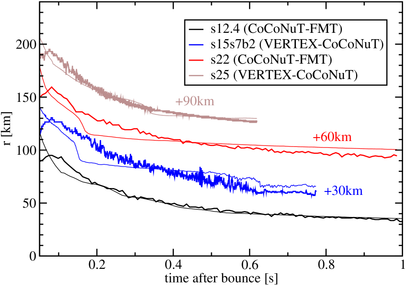
Figure 1: Comparison of the gain radius in models computed with the Vertex-CoCoNuT and CoCoNuT-FMT codes (thick lines) and the analytic contraction law (9) (thin lines) for progenitor models from Woosley et al. (2002) (black: s12.4, red: s22, light brown: s25) and Woosley & Weaver (1995) (blue: s15s7b2). All models have been computed using the nuclear equation of state of Lattimer & Swesty (1991) with a nuclear incompressibility modulus $K=220\,\mathrm{MeV}$, except for s15s7b2 ($K=180\,\mathrm{MeV}$). The Vertex models have been discussed previously in Müller et al. (2012a, 2013); Müller & Janka (2014). Note that the curves for s15s7b2, s22, and s25 are offset by $30\,\mathrm{km}$, $60\,\mathrm{km}$, and $90\,\mathrm{km}$, respectively. Overall, the analytic contraction law reproduces the contraction of the gain radius reasonably well. It somewhat overestimates the recession after the infall of composition interfaces with strong density jumps, which is more gradual in realistic models.

In this work, we use $r_{0}=12\,\mathrm{km}$ and $r_{1}=120\,\mathrm{km}$. Figure 1 shows that Equation (9) provides a reasonably good fit to the contraction of the proto-neutron star except for brief phases when the accretion rate drops abruptly after the infall of a shell interface.

The neutrino luminosity $L_{\nu}$ (of electron neutrinos and antineutrinos) is modelled as consisting of an accretion component $L_{\mathrm{acc}}$,

$$L_{\mathrm{acc}}=\zeta\frac{GM\dot{M}}{r_{\mathrm{g}}},$$ (10)

where the conversion of accretion energy into luminosity is specified by an adjustable efficiency parameter $\zeta$, and a diffusive component $L_{\mathrm{diff}}$ originating from deeper layers of the proto-neutron star (compare Fischer et al. 2009; Müller & Janka 2014). Based on the results of Müller & Janka (2014), we typically use $\zeta=0.7$. We estimate $L_{\mathrm{diff}}$ by assuming that the binding energy of a cold neutron star (Lattimer & Yahil, 1989; Lattimer & Prakash, 2001),

$$E_{\mathrm{bind}}\approx 0.084\,M_{\odot}c^{2}(M_{\mathrm{NS}}/M_{\odot})^{2}$$ (11)

is radiated away as diffusion luminosity over a time-scale $\tau_{\mathrm{cool}}$. Here $M_{\mathrm{NS}}$ is the gravitational mass of the neutron star. An additional power-law dependence on the baryonic neutron star mass is introduced for $\tau_{\mathrm{cool}}$ to account (somewhat ad hoc) for the fact that the higher densities, temperatures, and (for electron neutrinos) chemical potentials in high-mass neutron stars increase the diffusion time-scale,

$$\tau_{\mathrm{cool}}=\tau_{\mathrm{1.5}}\,\mathrm{s}\times\left(\frac{M}{1.5\,M_{\odot}}\right)^{5/3},$$ (12)

$$L_{\nu}=-0.3\dot{E}_{\mathrm{bind}}\approx 0.3\times\frac{E_{\mathrm{bind}}(M)}{\tau_{\mathrm{cool}}(M)}.$$ (13)

The pre-factor $0.3$ accounts for the fact that only roughly one third of the binding energy is emitted in the form of electron neutrinos and antineutrinos that contribute to neutrino heating in the gain layer. Moreover, the material accreted onto the proto-neutron star has already lost part of its binding energy as accretion luminosity in the cooling region. The value of the proportionality constant $\tau_{\mathrm{1.5}}$ (cooling time-scale for a $1.5\,M_{\odot}$ mass neutron star) has to be determined from simulations; the recent results of Hüdepohl (2014) suggest that $\tau_{1.5}\approx 1.2\,\mathrm{s}$. Our choice of parameters results in diffusion luminosities of a few $10^{52}\,\mathrm{erg}\,\mathrm{s}^{-1}$ and a tendency towards slightly higher diffusion luminosities for higher neutron star masses, which is in agreement with systematic studies of the progenitor dependence of the heavy flavour neutrino emission (O’Connor & Ott, 2013).

Neglecting secular changes in $M$ and $\tau_{\mathrm{cool}}$, we simply use the exponential solution for the diffusion luminosity for constant $M$ to estimate the instantaneous value of $L_{\mathrm{diff}}$:

$$L_{\mathrm{diff}}=E_{\mathrm{bind}}(M)e^{-t/\tau_{\mathrm{cool}}(M)}.$$ (14)

We note that $E_{\mathrm{bind}}$ (equation 11) can be expressed explicitly in terms of the current baryonic neutron star mass $M$ instead of the gravitational neutron star mass $M_{\mathrm{NS}}$,

$$E_{\mathrm{bind}}=\left(M-\frac{\left(-1+\sqrt{1+0.336\,M/M_{\odot}}\right)M_{\odot}}{0.168}\right)c^{2}.$$ (15)

For the total electron (anti-)neutrino luminosity, we also include a factor accounting for general relativistic redshift of neutrinos originating from close to the proto-neutron star radius:

$$L_{\mathrm{\nu}}=\sqrt{1-\frac{2GM}{r_{\mathrm{PNS}}}}(L_{\mathrm{acc}}+L_{\mathrm{diff}}),$$ (16)

where we use $r_{\mathrm{PNS}}\approx 5/7r_{\mathrm{g}}$. The redshift factor also needs to be applied to the neutrino mean energies.

Once the neutrino luminosity and mean energy and the gain radius are determined, we can formulate the second (inner) boundary condition for the pressure stratification in the gain region. If the neutrino heating and cooling rate per unit mass are to balance each other at the gain radius, we must have

$$T_{\mathrm{g}}^{6}\propto\frac{L_{\nu}E_{\nu}^{2}}{r_{\mathrm{g}}^{2}},$$ (17)

for the temperature $T_{\mathrm{g}}$ at the gain radius since the cooling and heating rates per baryon scale as $T^{6}\propto P^{3/2}$ and $L_{\nu}E_{\nu}^{2}/r_{\mathrm{g}}^{2}$, respectively. With $P_{\mathrm{g}}\propto T_{\mathrm{g}}^{4}$, the pressure at the gain radius $P_{\mathrm{g}}$ scales as,

$$P_{\mathrm{g}}^{3/2}\propto\frac{L_{\nu}E_{\nu}^{2}}{r_{\mathrm{g}}^{2}},$$ (18)

which is our second (inner) boundary condition for the pressure stratification in the gain region.

2.1.4 Solution for the Shock Radius

Solving Equations (5,18) using $P\propto r^{-4}$, we obtain a scaling relation for the shock radius (Janka, 2012),

$$r_{\mathrm{sh}}\propto\frac{(L_{\nu}E_{\nu}^{2})^{4/9}r_{\mathrm{g}}^{16/9}}{\dot{M}^{2/3}M^{1/3}}\propto\frac{L_{\nu}^{4/9}M^{5/9}r_{\mathrm{g}}^{16/9}}{\dot{M}^{2/3}},$$ (19)

where we have used $E_{\nu}\propto M$ to obtain the second form.

Multi-dimensional effects are not yet taken into account in this formula for the shock radius. Müller & Janka (2015) pointed out that the different multi-D effects that have been proposed as beneficial for shock revival, such as shock expansion due to turbulent stresses (Burrows et al., 1995; Murphy et al., 2013), the increased advection time-scale (Buras et al., 2006; Murphy & Burrows, 2008; Marek & Janka, 2009), and the increased heating efficiency compared to 1D are inseparably related and coupled to each other by feedback processes. They suggested that they can effectively be captured in a 1D model by modifying the equations for the hydrostatic structure and the jump conditions at the shock. To this end, they proposed to account for turbulent stresses in a rather simple fashion by a correction factor containing the root-mean-square averaged turbulent Mach number $\langle\mathrm{Ma}^{2}\rangle$ in the gain region,

$$r_{\mathrm{sh}}\rightarrow r_{\mathrm{sh}}\left(1+\frac{4\langle\mathrm{Ma}^{2}\rangle}{3}\right)^{2/3},$$ (20)

which then also implies an increase in $M_{\mathrm{g}}$ and hence in the heating efficiency (Equation 16 in Müller & Janka 2015) and the advection time-scale (see Equation 2.1.5 below). Using a large number of axisymmetric supernova simulations of different progenitors, Summa et al. (2015) recently showed that the effect of turbulent stresses on the critical neutrino luminosity required for shock revival can be captured remarkably well by such a simple modification.

Since we merely use the shock radius to solve for the point in time where the critical explosion condition $\tau_{\mathrm{adv}}/\tau_{\mathrm{heat}}=1$ is met, we may as well replace the turbulent Mach number with its critical value $\langle\mathrm{Ma}^{2}\rangle\approx 0.4649$ (Müller & Janka, 2015), which implies that the shock radius obtained from Equation (19) can be consistently multiplied with a constant factor $\alpha_{\mathrm{turb}}$,

$$r_{\mathrm{sh}}\rightarrow\alpha_{\mathrm{turb}}r_{\mathrm{sh}}.$$ (21)

Müller & Janka (2015) derived a value of $\alpha_{\mathrm{turb}}\approx 1.38$ in the absence of strong seed perturbations in the progenitor, which they found to be in good agreement with 2D simulations. There is obviously justification for varying $\alpha_{\mathrm{turb}}$ within reasonable bounds on several grounds: While the underlying scaling law for the turbulent Mach number likely holds in 3D as well, the relevant dimensionless efficiency parameters (e.g. for turbulent dissipation) and hence $\alpha_{\mathrm{turb}}$ are bound to be slightly different, although the difference in $\alpha_{\mathrm{turb}}$ between 2D and 3D cannot be excessive given that the critical luminosity is very similar in both cases (Hanke et al., 2012; Dolence et al., 2013; Couch, 2013; Handy et al., 2014). Moreover, since the record of 3D supernova simulations in obtaining explosions is mixed so far, and some crucial ingredients that boost the turbulent motions behind the shock may still be missing (such as strong seed perturbations from convective burning in the progenitor; Couch & Ott 2013; Couch et al. 2015; Müller & Janka 2015), Finally, since our fits for the shock radius, and the advection and heating time-scales are already based on 2D and 3D simulations, and since the fits never perfectly reproduce the heating conditions in self-consistent models, $\alpha_{\mathrm{turb}}$ needs to be renormalised, and we will use values in the range $\alpha_{\mathrm{turb}}=1.08\ldots 1.28$ with a standard value of $\alpha_{\mathrm{turb}}=1.18$. Because of this renormalisation, $\alpha_{\mathrm{turb}}=1$ no longer has any special significance, and cannot be interpreted as the limit where multi-D effects are “switched off”. Using the theoretically inferred value of $\alpha_{\mathrm{turb}}\approx 1.38$ at shock revival in multi-D, the “1D” limit would more likely correspond to $\alpha_{\mathrm{turb}}\approx 0.86$, in which case we only obtain four explosions at the lower mass end, which is not implausible and in line with the fact that 1D simulations do not show explosions except at the low-mass end (Kitaura et al., 2006; Janka et al., 2008; Fischer et al., 2010; Melson et al., 2015a). This finding should not be interpreted as more than a rough consistency check for our model, since the role of multi-D effects is a lot more subtle in reality.

The proportionality constants for the final scaling law for $r_{\mathrm{sh}}$ are once again chosen to obtain a good fit to simulation results,

$$r_{\mathrm{sh}} = \alpha_{\mathrm{turb}}\times 55\,\mathrm{km}\times\left(\frac{L_{\nu}}{10^{52}\,\mathrm{erg}\,\mathrm{s}^{-1}}\right)^{4/9}\times\left(\frac{M}{M_{\odot}}\right)^{5/9}$$ (22)

$$\times\left(\frac{r_{\mathrm{g}}}{10\,\mathrm{km}}\right)^{16/9}\times\left(\frac{\dot{M}}{M_{\odot}\,\mathrm{s}^{-1}}\right)^{-2/3}.$$

2.1.5 Heating Conditions

From the shock radius, we immediately find a scaling law for the advection time-scale,

$$\tau_{\mathrm{adv}} = \frac{M_{\mathrm{g}}}{\dot{M}}=\frac{\int_{r_{\mathrm{g}}}^{r_{\mathrm{sh}}}4\pi r^{2}\beta\rho_{\mathrm{pre}}(r_{\mathrm{sh}}/r)^{3}\,\mathrm{d}r}{\dot{M}}$$

$$\approx 18\,\mathrm{ms}\left(\frac{r_{\mathrm{sh}}}{100\,\mathrm{km}}\right)^{3/2}\left(\frac{M}{M_{\odot}}\right)^{-1/2}\ln\frac{r_{\mathrm{sh}}}{r_{\mathrm{g}}},$$

where the proportionality constant has been chosen to fit the results of first-principle simulations (Müller & Janka, 2015).

The heating time-scale $\tau_{\mathrm{heat}}$ can be expressed in terms of the average mass-specific neutrino heating rate $\dot{q}_{\nu}$ and the average net binding energy (i.e., thermal, kinetic, and potential energy) $e_{\mathrm{g}}$ of matter in the gain region. It is relatively easy to obtain a robust scaling law for $\dot{q}_{\nu}$ (Janka, 2001, 2012; Müller & Janka, 2015),

$$\dot{q}_{\nu}\propto\frac{L_{\nu}E_{\nu}^{2}}{r_{\mathrm{g}}^{2}}.$$ (24)

The average binding energy is a slightly more complicated case. Neither the assumption of a constant, time-independent binding energy (Müller & Janka, 2015), nor the assumption that $e_{\mathrm{g}}$ scales with the gravitational potential energy at the shock (Janka, 2012) provides an optimal fit to simulation results. A better estimate for $e_{\mathrm{g}}$ can be obtained by invoking Bernoulli’s theorem for a stationary compressible flow in spherical symmetry (Müller, 2015): Since the sum of the total enthalpy $h$ (including rest-mass contributions), the kinetic energy density, and the gravitational potential are conserved during the infall, it is roughly equal to its (negligibly small) value at the initial position of a given mass shell,

$$h+v^{2}/2+\Phi=0,$$ (25)

Neglecting the kinetic energy in the post-shock region, we therefore find

$$\epsilon_{\mathrm{therm}}+\epsilon_{\mathrm{diss}}+\frac{P_{\mathrm{sh}}}{\rho_{\mathrm{sh}}}-\frac{GM}{r_{\mathrm{sh}}}\approx 0,$$ (26)

for the thermal energy per unit mass $\epsilon_{\mathrm{therm}}$ just behind the shock. Note that rest-mass contributions are excluded from $\epsilon_{\mathrm{therm}}$ and lumped into the dissociation energy $\epsilon_{\mathrm{diss}}$. With radiation pressure dominating in the post-shock region, we have $P_{\mathrm{sh}}/\rho_{\mathrm{sh}}=\epsilon_{\mathrm{therm}}/3$, and hence obtain

$$\frac{4}{3}\epsilon_{\mathrm{therm}}+\epsilon_{\mathrm{diss}}=\frac{GM}{r_{\mathrm{sh}}},$$ (27)

$$\epsilon_{\mathrm{therm}}=\frac{3}{4}\left(\frac{GM}{r_{\mathrm{sh}}}-\epsilon_{\mathrm{diss}}\right),$$ (28)

which leads to

$$|e_{\mathrm{g}}|=\left|\epsilon_{\mathrm{therm}}-\frac{GM}{r_{\mathrm{sh}}}\right|=\frac{3}{4}\epsilon_{\mathrm{diss}}+\frac{GM}{4r_{\mathrm{sh}}},$$ (29)

for the post-shock binding energy without rest-mass contributions. Assuming complete dissociation of the infalling heavy nuclei into nucleons, we have $\epsilon_{\mathrm{diss}}\approx 8.8\,\mathrm{MeV}$. Note that the value of the total energy per unit mass immediately behind the shock is used as a proxy for the entire gain region.

After combining Equations (24) and (29) and choosing the appropriate value for the proportionality constant, we obtain our final expression for the heating time-scale,

$$\tau_{\mathrm{heat}} = 150\,\mathrm{ms}\times\left(\frac{|e_{\mathrm{g}}|}{10^{19}\,\mathrm{erg}\,\mathrm{g}^{-1}}\right)\times\left(\frac{r_{\mathrm{g}}}{100\,\mathrm{km}}\right)$$

$$\times\left(\frac{L_{\nu}}{10^{52}\,\mathrm{erg}\,\mathrm{s}^{-1}}\right)^{-1}\times\left(\frac{M}{M_{\odot}}\right)^{-2}$$

We note that Equations (22,2.1.5,2.1.5) also implicitly determine the mass in the gain region $M_{\mathrm{g}}$, the average neutrino heating rate per unit mass $\dot{q}_{\nu}$ and the volume-integrated neutrino heating rate $\dot{Q}_{\nu}=\dot{q}_{\nu}M_{\mathrm{g}}$. For our treatment of the explosion phase, it will be convenient to define an efficiency parameter $\eta_{\mathrm{acc}}$ relating the mass accretion rate $\dot{M}$ onto the proto-neutron star to the volume-integrated heating rate $\dot{Q}_{\nu}$,

$$\eta_{\mathrm{acc}}=\frac{\dot{Q}_{\nu}}{\dot{M}}.$$ (31)

2.2 Explosion Phase

The analytic model for the heating conditions during the pre-explosion phase presented in Section 2.1 allows us to compute the critical time-scale ratio $\tau_{\mathrm{adv}}/\tau_{\mathrm{heat}}$ as a function of the mass coordinate of the infalling shells. If we find $\tau_{\mathrm{adv}}/\tau_{\mathrm{heat}}<1$ throughout the star or at least for all $M$ smaller than the (unknown) maximum baryonic neutron star mass $M_{\mathrm{max}}$, we assume that a stellar model forms a black hole without ever undergoing shock revival. In this work, we use a maximum gravitational neutron star mass of $2.05\,M_{\odot}$, which is compatible with the best current lower limits for $M_{\mathrm{max}}$ (Antoniadis et al., 2013; Demorest et al., 2010).

Otherwise, we take the minimum $M$ for which $\tau_{\mathrm{adv}}/\tau_{\mathrm{heat}}=1$ as an “initial mass cut” $M_{\mathrm{ini}}$ and then proceed to estimate the residual accretion onto the proto-neutron star and the explosion parameters. We achieve this by relating the amount of accretion after shock revival, the shock propagation, and the energetics of the incipient explosion (quantified by the “diagnostic explosion energy”, viz. the total energy of the material that is nominally unbound at a given stage after shock revival) to each other.

2.2.1 Accretion after Shock Revival

Except for the least massive supernova progenitors (Kitaura et al., 2006; Müller et al., 2012b), successful first-principle simulations of supernova explosions (Buras et al., 2006; Marek & Janka, 2009; Müller et al., 2012a, b, 2013; Müller & Janka, 2014; Janka et al., 2012; Bruenn et al., 2013, 2016; Suwa et al., 2010; Nakamura et al., 2015; Takiwaki et al., 2012, 2014; Summa et al., 2015; O’Connor & Couch, 2015) consistently show the persistence of accretion downflows for many hundreds of milliseconds after shock revival — and in many cases to the very end of the simulations so that the final explosion parameters of the models cannot be determined yet. A more quantitative analysis of the mass fluxes $\dot{M}_{\mathrm{out}}$ and $\dot{M}_{\mathrm{acc}}$ in neutrino-driven outflows and cold accretion downflows in the long-time simulations of Müller (2015) revealed that the accretion through downflows completely outweighs the outflow rate for a long time,

$$\dot{M}_{\mathrm{acc}}\gg\dot{M}_{\mathrm{out}}.$$ (32)

While the long persistence of accretion is a major technical obstacles for simulations, it simplifies the treatment of the post-explosion phase in the sense that it allows us to use the same estimate for the accretion rate onto the proto-neutron star (and hence for the neutron star contraction, the neutrino luminosity, and the neutrino heating rate) as in the pre-explosion phase. During this initial phase of the explosion (henceforth called phase I of the explosion), the primary contribution to the explosion energy comes from neutrino-heated outflows that are driven by a relatively high accretion luminosity.

Eventually, the residual accretion will cease and Equation (32) breaks down. In the subsequent phase (phase II of the explosion), the proto-neutron star will still radiate neutrinos as it cools over a time-scale of several seconds, and the neutrino-driven wind will still contribute somewhat to the explosion energy.

One can estimate that the transition from phase I to phase II occurs roughly when the newly shocked material is accelerated to the local escape velocity (Marek & Janka, 2009) because this precludes accretion onto the neutron star on a short time-scale (although the interaction with the rest of the ejecta may still lead to late-time fallback). This can be translated into a condition for the shock velocity: At the transition point, the shock will already have propagated to several thousands or even tens of thousands of kilometres and the immediate post-shock velocity will be high compared to the small pre-shock infall velocity. For a negligible pre-shock velocity, the post-shock velocity $v_{\mathrm{post}}$ of the newly shocked material is given in terms of the shock velocity $v_{\mathrm{sh}}$ and the compression ratio $\beta_{\mathrm{expl}}$ as

$$v_{\mathrm{post}}=\frac{\beta_{\mathrm{expl}}-1}{\beta_{\mathrm{expl}}}v_{\mathrm{sh}}.$$ (33)

Accretion will thus subside roughly once the criterion

$$\frac{\beta_{\mathrm{expl}}-1}{\beta_{\mathrm{expl}}}v_{\mathrm{sh}}=\sqrt{\frac{2GM}{r}}$$ (34)

is met. The radius $r$ in this equation is the initial radius of the mass shell $M$, which cannot have moved very far from its initial position when it is hit by the shock. Furthermore, we note that the compression ratio $\beta_{\mathrm{expl}}$ in the explosion phase can be different from the pre-explosion phase and will generally be smaller than the compression ratio $\beta=(\gamma+1)/(\gamma-1)$ for an ideal gas with a $\gamma$-law equation of state because of nuclear burning in the shock. Values around $\beta_{\mathrm{expl}}=4$ are typical for the early explosion phase (Müller, 2015).

2.2.2 Shock Velocity

The propagation of the shock depends on the energetics of the explosion. Müller (2015) showed that despite the enormously complicated multi-dimensional flow structure after shock revival, it turns out that the average shock velocity (defined as the time derivative of the average shock radius $r_{\mathrm{sh}}$) closely follows the analytic formula derived by Matzner & McKee (1999) for shock propagation in spherical symmetry,

$$v_{\mathrm{sh}}=0.794\left(\frac{E_{\mathrm{diag}}}{M-M_{\mathrm{ini}}}\right)^{1/2}\left(\frac{M-M_{\mathrm{ini}}}{\rho r^{3}}\right)^{0.19}.$$ (35)

Here, $E_{\mathrm{diag}}$ is the diagnostic explosion energy, and the density $\rho$ and radius $r$ again refer to the initial progenitor model.

2.2.3 Evolution of Explosion and Remnant Parameters– Phase I

Combined with a model for the evolution of the diagnostic explosion energy in phase I and phase II, we can use Equations (34) and (35) to determine both the amount of residual accretion (and hence the final neutron star mass) as well as the final explosion energy.

During phase I, both strong neutrino heating powered by the accretion downflows as well as nuclear burning in the shock contribute to the explosion energy. Simulation results suggest that the contribution from neutrino heating can be estimated as follows: As the outflowing material just barely reaches positive total energy, the outflow rate is roughly given by the ratio of the volume-integrated neutrino-heating rate $\dot{Q}_{\nu}$ and the initial binding energy at the gain radius $|e_{\mathrm{g}}|$,

$$\dot{M}_{\mathrm{out}}=\frac{\eta_{\mathrm{out}}\dot{Q}_{\nu}}{|e_{\mathrm{g}}|}=\frac{\eta_{\mathrm{out}}\eta_{\mathrm{acc}}\dot{M}_{\mathrm{acc}}}{|e_{\mathrm{g}}|}.$$ (36)

Here, $\eta_{\mathrm{out}}$ is a dimensionless efficiency parameter for the conversion of neutrino heating into an outflow rate. The recent 3D simulation of Müller (2015) suggests $\eta_{\mathrm{out}}=1$, and we adopt this value throughout our work. $\eta_{\mathrm{out}}$ needs to be carefully distinguished from the surface fraction $\alpha_{\mathrm{out}}$ occupied by neutrino-driven outflows far away from the gain radius, which we will need later. Note that we use the heating rate computed in Section 2.1 during the pre-explosion phase because the accretion onto the proto-neutron star and hence the neutrino heating are hardly affected by the outflows initially.

The energy input by neutrino heating into the outflow is essentially used up completely to unbind the material, and the net contribution from the explosion energy comes from the recombination of nucleons (compare Scheck et al. 2006; Müller et al. 2012a). Therefore, the evolution of the diagnostic explosion energy $E_{\mathrm{diag}}$ is given by

$$\dot{E}_{\mathrm{diag}}=\epsilon_{\mathrm{rec}}\dot{M}_{\mathrm{out}},$$ (37)

where $\epsilon_{\mathrm{rec}}$ is the recombination energy. For recombination into iron group nuclei, we would have $\epsilon_{\mathrm{rec}}\approx 8.8\,\mathrm{MeV}$, but for the high entropies in neutrino-driven outflows, recombination will mostly go into $\alpha$-particles and not to iron group nuclei, and some of the energy gained from recombination is lost due to turbulent energy exchange between the outflows and downflows (Müller, 2015). In this work, we therefore use the value of $\epsilon_{\mathrm{rec}}\approx 5\,\mathrm{MeV}$ found by Müller (2015) for the asymptotic total energy of the neutrino-heated ejecta.

It is convenient to rewrite Equation (37) as an equation for the time derivative $\mathrm{d}E_{\mathrm{expl}}/\mathrm{d}M_{\mathrm{sh}}$ instead, where $M_{\mathrm{sh}}$ is the mass coordinate reached by the shock at a given time. Assuming that a fraction $1-\alpha_{\mathrm{out}}$ (where $\alpha_{\mathrm{out}}$ is the surface fraction occupied by neutrino-driven outflows) of the shocked material is eventually accreted, the diagnostic energy should grow as

$$\frac{\mathrm{d}E_{\mathrm{diag}}}{\mathrm{d}M_{\mathrm{sh}}}=\epsilon_{\mathrm{rec}}\frac{\mathrm{d}{M}_{\mathrm{out}}}{\mathrm{d}{M}_{\mathrm{acc}}}\frac{\mathrm{d}M_{\mathrm{acc}}}{\mathrm{d}M_{\mathrm{sh}}}=\frac{(1-\alpha_{\mathrm{out}})\epsilon_{\mathrm{rec}}\eta_{\mathrm{acc}}}{|e_{\mathrm{g}}|}.$$ (38)

While the eventual contribution to the explosion energy from the accretion of a given mass shell can be computed according to Equation (38), the diagnostic explosion energy will still be lower at the time when the mass shell is shocked, and this lower value is needed to determine (via the post-shock velocity) when accretion subsides.

To calculate the diagnostic energy $E_{\mathrm{imm}}$ at the time when the shock reaches a given mass shell, we assume that the accretion rate at this point is still given by Equation (32) as for non-exploding models. Since the shock sweeps up matter at a rate of $\mathrm{d}M_{\mathrm{sh}}/\mathrm{d}t=4\pi r^{2}v_{\mathrm{sh}}\rho$, we obtain

$$\frac{\mathrm{d}E_{\mathrm{imm}}}{\mathrm{d}M_{\mathrm{sh}}} = \frac{\mathrm{d}E_{\mathrm{imm}}}{\mathrm{d}t}\frac{\mathrm{d}t}{\mathrm{d}M_{\mathrm{sh}}}=\frac{1}{4\pi r^{2}v_{\mathrm{sh}}\rho}\frac{\mathrm{d}E_{\mathrm{diag}}}{\mathrm{d}t}$$ (39)

$$= \frac{1}{4\pi r^{2}v_{\mathrm{sh}}\rho}\frac{\epsilon_{\mathrm{rec}}\dot{Q}_{\nu}}{|e_{\mathrm{g}}|}=\frac{\epsilon_{\mathrm{rec}}\eta_{\mathrm{acc}}\dot{M}}{4\pi r^{2}v_{\mathrm{sh}}\rho|e_{\mathrm{g}}|},$$ (40)

in the regime where the shock velocity is considerably larger than the pre-shock infall velocity. Immediately after shock revival, this is not the case, and we can instead assume that the shocked matter is immediately accreted onto the proto-neutron star. To accommodate both regimes, we solve the following equation for $E_{\mathrm{imm}}$,

$$\frac{\mathrm{d}E_{\mathrm{imm}}}{\mathrm{d}M_{\mathrm{sh}}}=\frac{\epsilon_{\mathrm{rec}}\eta_{\mathrm{acc}}}{|e_{\mathrm{g}}|}\min\left(1,\frac{\dot{M}}{4\pi r^{2}v_{\mathrm{sh}}\rho}\right).$$ (41)

$E_{\mathrm{imm}}$ is then used to compute the shock velocity according to Equation (35) and to determine the amount of explosive burning (see below).

Aside from energy input by neutrino heating, we also need to take into account that the shocked material is initially bound and that nuclear burning in the shock contributes to the explosion energy provided that the post-shock temperatures are high enough. It is straightforward to take this into account by including additional source terms $\epsilon_{\mathrm{bind}}$ for the binding energy per unit mass of the unshocked material and $\epsilon_{\mathrm{burn}}$ for nuclear burning,

$$\frac{\mathrm{d}E_{\mathrm{diag}}}{\mathrm{d}M_{\mathrm{sh}}}=\frac{(1-\alpha_{\mathrm{out}})\epsilon_{\mathrm{rec}}\eta_{\mathrm{acc}}}{|e_{\mathrm{g}}|}+\alpha_{\mathrm{out}}\left(\epsilon_{\mathrm{bind}}+\epsilon_{\mathrm{burn}}\right).$$ (42)

Unlike neutrino heating powered by the accretion of shocked material, $\epsilon_{\mathrm{bind}}$ and $\epsilon_{\mathrm{burn}}$ contribute to the explosion energy without any delay, so that the equation for $E_{\mathrm{imm}}$ becomes:

$$\frac{\mathrm{d}E_{\mathrm{imm}}}{\mathrm{d}M_{\mathrm{sh}}} = \frac{\epsilon_{\mathrm{rec}}\eta_{\mathrm{acc}}}{|e_{\mathrm{g}}|}\min\left(1,\frac{\dot{M}}{4\pi r^{2}v_{\mathrm{sh}}\rho}\right)$$ (43)

$$+\alpha_{\mathrm{out}}\left(\epsilon_{\mathrm{bind}}+\epsilon_{\mathrm{burn}}\right).$$

Note that $\epsilon_{\mathrm{bind}}$ and $\epsilon_{\mathrm{burn}}$ are multiplied with the surface fraction occupied by outflows, $\alpha_{\mathrm{out}}$, to account for the fact that some of the shocked material is channelled into downflows and not swept up by the ejecta.

$\epsilon_{\mathrm{burn}}$ is given in terms of the initial and final mass fractions $X_{i}$ and $X^{\prime}_{i}$ prior to and after explosive burning and the rest-mass contributions $\epsilon_{\mathrm{rm}}$ per unit mass for nucleus $i$,

$$\epsilon_{\mathrm{burn}}=\sum_{i}(X_{i}-X^{\prime}_{i})\epsilon_{\mathrm{rm},i}.$$ (44)

To obtain $X_{i}$, we apply the “flashing” method of Rampp & Janka (2002), i.e., we assume that the different burning processes (C-, O-, Si-burning) occur instantaneously at certain ignition temperatures. To this end, we compute the post-shock temperature $T_{\mathrm{sh}}$ by assuming that radiation pressure dominates behind the shock and that the infall velocity is negligible compared to the shock velocity. With the post-shock pressure $P_{\mathrm{sh}}$ determined by the jump conditions, we then obtain

$$P_{\mathrm{sh}}=\frac{aT_{\mathrm{sh}}^{4}}{3}=\frac{\beta_{\mathrm{expl}}-1}{\beta_{\mathrm{expl}}}\rho v_{\mathrm{sh}}^{2},$$ (45)

or,

$$T_{\mathrm{sh}}=\sqrt[4]{\frac{3\beta_{\mathrm{expl}}-1}{a\beta_{\mathrm{expl}}}\rho v_{\mathrm{sh}}^{2}},$$ (46)

where $a$ is the radiation constant.

Depending on the post-shock temperature $T_{\mathrm{sh}}$, the initial composition is then changed as follows:

1. For $2.5\times 10^{9}\,\mathrm{K}\leq T_{\mathrm{sh}}<3.5\times 10^{9}\,\mathrm{K}$, we burn elements lighter than O to ${}^{16}\mathrm{O}$.

2. For $3.5\times 10^{9}\,\mathrm{K}\leq T_{\mathrm{sh}}<5\times 10^{9}\,\mathrm{K}$, we burn elements lighter than Si to ${}^{28}\mathrm{Si}$.

3. For $5\times 10^{9}\,\mathrm{K}\leq T_{\mathrm{sh}}<T_{\alpha}$, we burn everything to ${}^{56}\mathrm{Ni}$. Note that we follow Iliadis (2007) in choosing a different temperature threshold for complete Si than Rampp & Janka (2002).

Here $T_{\alpha}$ denotes the density-dependent temperature for which the mass fraction of $\alpha$-particles reaches $0.5$ in nuclear statistical equilibrium. $T_{\alpha}$ is implicitly given by (Shapiro & Teukolsky, 1983; Rampp & Janka, 2002),

$$\log_{10}\rho=11.62+1.5\log_{10}\left(\frac{T_{\alpha}}{10^{9}\,\mathrm{K}}\right)-39.17\left(\frac{T_{\alpha}}{10^{9}\,\mathrm{K}}\right)^{-1}.$$ (47)

The proto-neutron star also grows due to continued accretion during phase I. The fraction of the shocked material that ends up in the proto-neutron star roughly corresponds to the surface fraction of the downflows. Moreover, a fraction $\eta_{\mathrm{acc}}/|e_{\mathrm{g}}|$ of the accreted material is re-ejected by neutrino heating, so that we obtain the following differential equation for the (baryonic) neutron star mass $M_{\mathrm{by}}$ as a function of $M_{\mathrm{sh}}$,

$$\frac{dM_{\mathrm{by}}}{dM_{\mathrm{sh}}}=(1-\alpha_{\mathrm{out}})(1-\eta_{\mathrm{acc}}/|e_{\mathrm{g}}|)$$ (48)

.

Using Equations (34,35,42,48), we can follow the evolution of the explosion energy and determine the mass $M_{\mathrm{by}}$ of the proto-neutron star at the end of phase I.

2.2.4 Evolution of Explosion and Remnant Parameters– Phase II

During phase II, the explosion energy can still change due to explosive burning in the shock, the accumulation of bound material by the shock, and the energy input from the neutrino-driven wind (which also reduces the proto-neutron star mass).

In recent self-consistent simulations of the wind phase in electron capture supernova explosion (Janka et al., 2008; von Groote, 2014), the wind contributes only $\mathord{\sim}10^{48}\,\mathrm{erg}$ to the explosion energy and the integrated mass loss is $\Delta M_{\mathrm{wind}}\lesssim 10^{-4}\,M_{\odot}$. Even for more massive progenitors that leave behind more massive neutron stars with hotter neutrinospheres, the integrated mass loss in the wind remains well below $10^{-3}\,M_{\odot}$ (Hüdepohl, 2014), implying a contribution to the explosion energy of $\ll 10^{50}\,\mathrm{erg}$.

We therefore feel justified in neglecting the effect of the neutrino-driven wind on the final explosion and remnant properties in this work, and consider only the two remaining contributions. Aside from the fact that all of the matter swept up by the shock now contributes to the energy budget of the ejecta (and not just a fraction $\alpha_{\mathrm{out}}$), these can be treated exactly as in phase I, and the equation for the explosion energy becomes,

$$\frac{\mathrm{d}E_{\mathrm{diag}}}{\mathrm{d}M_{\mathrm{sh}}}=\epsilon_{\mathrm{bind}}+\epsilon_{\mathrm{burn}}.$$ (49)

The baryonic remnant mass $M$ is left unchanged during this phase.

2.2.5 Final Explosion Properties and Neutron Star Mass

Integrating Equation (49) out to the stellar surface yields the final explosion energy $E_{\mathrm{expl}}$. If $E_{\mathrm{expl}}$ is positive, we compute the final gravitational mass $M_{\mathrm{NS}}$ of the neutron star using the approximate formula (Lattimer & Yahil, 1989; Lattimer & Prakash, 2001)

$$M_{\mathrm{NS}}=M_{\mathrm{by}}-0.084\,M_{\odot}(M_{\mathrm{NS}}/M_{\odot})^{2}.$$ (50)

If $E_{\mathrm{diag}}$ becomes negative at any $M_{\mathrm{sh}}$, if the remnant mass $M_{\mathrm{NS}}$ exceeds the maximum neutron star mass $M_{\mathrm{max}}$, or (as discussed earlier) if the condition $\tau_{\mathrm{adv}}/\tau_{\mathrm{heat}}=1$ was never met, we assume that the entire star collapses to a black hole and set $E_{\mathrm{expl}}=0$. In that case, the gravitational remnant mass $M_{\mathrm{BH}}$ is set to the pre-collapse mass of the star. This is only a very crude estimate, and in the presentation of our results, we include $M_{\mathrm{BH}}$ primarily to indicate non-exploding models without attaching too much significance to the actual values. Even without shock revival, the actual black hole mass could be lower because the reduction of the gravitational mass of the interior shells by neutrino losses could lead to the (partial) ejection of the hydrogen envelope (Nadezhin, 1980; Lovegrove & Woosley, 2013), so that the helium core mass may be the more appropriate estimator for the black hole mass (Sukhbold & Woosley, 2014). Moreover, the possibility of fallback is considered only as an all-or-nothing event – it will involve the entire star if the diagnostic energy becomes negative, and no fallback is assumed to happen for successful explosions. The reality is thus obviously more complicated than our model, and the systematics of fallback will need to be studied in greater detail in a future continuation of this work.

During phase I and phase II, we also integrate the mass of iron group elements $M_{\mathrm{IG}}$ produced by explosive nuclear burning (taking into account that only a fraction $\alpha_{\mathrm{out}}$ out these will be ejected during phase I). $M_{\mathrm{IG}}$ can be taken as a rough proxy for the nickel mass, but needs to be interpreted with caution: ${}^{56}\mathrm{Ni}$ is not the only iron group element produced by explosive burning at sufficiently high temperatures, and the very crude “flashing” treatment based on an estimate of the post-shock temperature cannot be expected to yield quantitatively reliable results. For these reasons, $M_{\mathrm{IG}}$ can at best be expected to agree with the actual nickel mass within a factor of $\mathord{\sim}2$.

Table 1: Adjustable model parameters.

parameter	explanation	standard value	typical range
$\alpha_{\mathrm{out}}$	volume fraction of outflows	$0.5$	$0.3\ldots 0.7$
$\alpha_{\mathrm{turb}}$	shock expansion due to turbulent stresses	$1.18$	$1\ldots 1.4$
$\beta_{\mathrm{expl}}$	shock compression ratio during explosion phase	$4$	$3\ldots 7$
$\zeta$	efficiency factor for conversion of accretion energy into $\nu$ luminosity	$0.8$	$0.5\ldots 1$
$\tau_{1.5}$	cooling time-scale for $1.5\,M_{\odot}$ neutron star	$1.2\,\mathrm{s}$	$0.6\,\mathrm{s}\ldots 3\,\mathrm{s}$

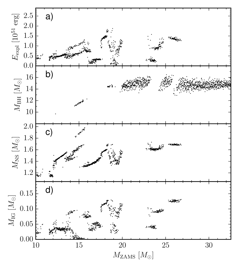
Figure 2: Explosion energy ($E_{\mathrm{expl}}$, Panel a), gravitational remnant masses for black holes ($M_{\mathrm{BH}}$, Panel b), neutron stars ($M_{\mathrm{NS}}$, Panel c), and the iron-group mass ($M_{\mathrm{IG}}$, Panel d) as a function of ZAMS mass for the standard case. Note that there is a gap in our set of progenitors around $11\,M_{\odot}$; missing data points in this region are not indicative of black hole formation.

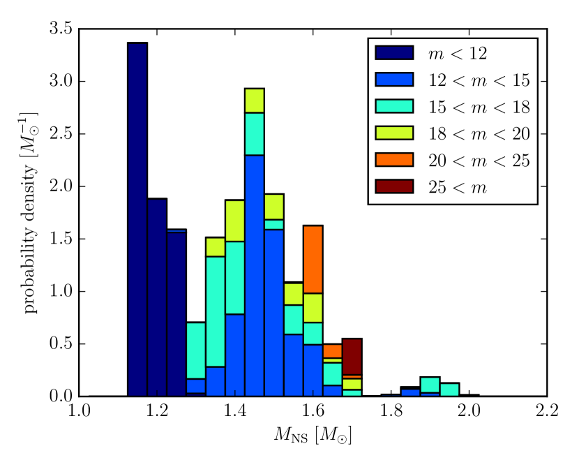
Figure 3: Histogram of the distribution of gravitational neutron star masses for the standard case. The stacked bars in different colours give the contribution of progenitors from different ranges of the ZAMS mass $m$ (measured in solar masses) to the average probability density in a given bin.

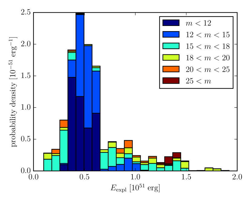
Figure 4: Histogram of the distribution of explosion energies for the standard case. The stacked bars in different colours give the contribution of progenitors from different ranges of the ZAMS mass $m$ (measured in solar masses) to the average probability density in a given bin.

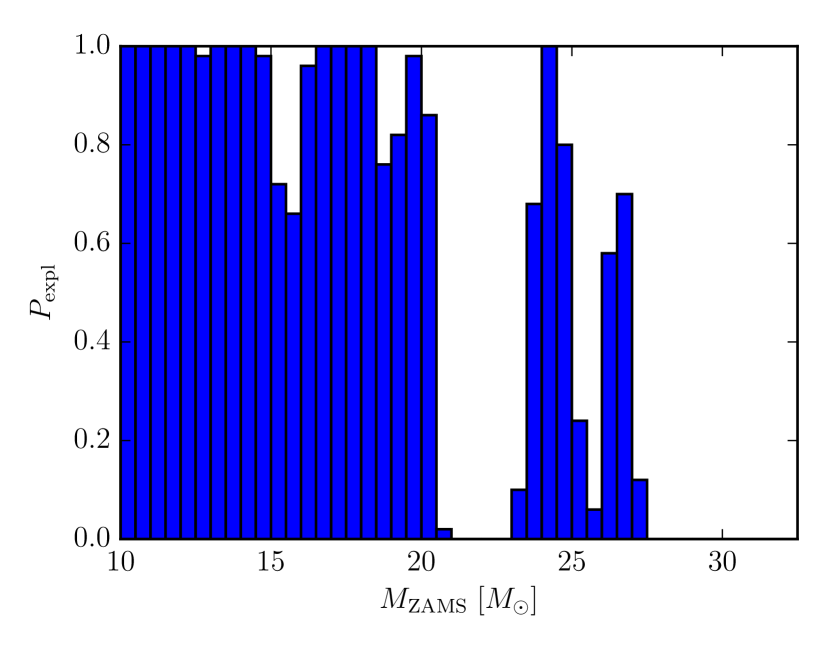
Figure 5: Fraction $P_{\mathrm{expl}}$ of successful explosions within bins of $0.5\,M_{\odot}$ for the standard case. There are no models in the bin between $11\,M_{\odot}$ and $11.5\,M_{\odot}$, but we assume that $P_{\mathrm{expl}}$ can be interpolated in this region, i.e., that there is no black hole formation.

3 Results

We apply our model to a set of 2120 solar-metallicity progenitor models computed with an up-to-date version of the stellar evolution code Kepler (Weaver et al., 1978; Heger & Woosley, 2010). The models cover a range from $10\,M_{\odot}$ and $32\,M_{\odot}$ in ZAMS mass with a typical spacing of $0.01\,M_{\odot}$ except for the mass range between $11\,M_{\odot}$ and $11.5\,M_{\odot}$, where not all of the models could be run up to collapse because of time constraints (see Woosley & Heger 2007, 2015b for a more detailed study of the lowest-mass supernova progenitors at solar metallicity). The input physics is very similar to the models of Sukhbold & Woosley (2014) and Sukhbold et al. (2016), except for updates in the neutrino loss rates (Itoh et al., 1996) and the initial solar composition (Asplund et al., 2009). The overall effect of these updates is a downward shift of the transition of structural features in the pre-SN evolution (like the transition between convective and radiative central carbon burning) by $\mathord{\approx}1.5\,M_{\odot}$ in ZAMS mass.

The analytic/ODE model has been implemented in Python 3. Once the Kepler model files are loaded, all progenitors can be processed within $35\,\mathrm{s}$ on a modern laptop computer. As our standard set of parameters, we adopt values of $\beta_{\mathrm{expl}}=4$, $\zeta=0.7$, $\alpha_{\mathrm{out}}=0.5$, $\alpha_{\mathrm{turb}}=1.18$, and $\tau_{1.5}=1.2\,\mathrm{s}$ for the five adjustable parameters of the model. Different from some coefficients and parameters that have implicitly been fixed in the preceding section, these parameters are beset with larger uncertainties, and we therefore explore variations itof each of these within a reasonable and justifiable range. Limits for the different parameters are listed in Table 1 along with our preferred values. These limits represent extremes that could be justified under certain physical assumptions (e.g., a strong reduction of neutrino opacities); if we require agreement with observational constraints the limits are in fact much tighter. We shall first discuss salient features of the explosion and remnant properties for our standard case before exploring the sensitivity to such parameter variations in Section 3.4.

3.1 Landscape of Neutron Star and Black Hole Formation – Standard Case

Figure 2 shows the explosion energy $E_{\mathrm{expl}}$, the gravitational mass of the remnant ($M_{\mathrm{NS}}$ for neutron stars and $M_{\mathrm{BH}}$ for black holes), and the estimated mass $M_{\mathrm{IG}}$ of iron group elements in the ejecta as a function of ZAMS mass, and the distribution of the explosion and remnant properties is further illustrated by IMF-weighted histograms in Figure 3 for $M_{\mathrm{NS}}$ and Figure 4 for $E_{\mathrm{expl}}$. We find a range of explosion energies from a few $10^{49}\,\mathrm{erg}$ to above $2\times 10^{51}\,\mathrm{erg}$, neutron star masses between $1.15\,M_{\odot}$ and $2\,M_{\odot}$, and iron group masses up to $0.15\,M_{\odot}$ similar to the parameterised 1D studies of Ugliano et al. (2012); Ertl et al. (2016) and Sukhbold et al. (2016). Different from these works, we do not include blue supergiant progenitors for the well-studied case of SN 1987A as a benchmark case. Given the uncertainty in the provenance of SN 1987A, whose progenitor may have originated from a merger event (Podsiadlowski & Joss, 1989; Podsiadlowski et al., 1990), and the range of stellar evolution models available for SN 1987A (see, e.g., Sukhbold et al., 2016), the only firm constraints that can be derived from this event is that some progenitor in the mass range between $15\,M_{\odot}$ and $20\,M_{\odot}$ with a helium core mass of $\sim 6\,M_{\odot}$ should explode with an energy of $(1\ldots 1.5)\times 10^{51}\,\mathrm{erg}$ and produce $\sim 0.07\,M_{\odot}$ of nickel (Shigeyama & Nomoto, 1990; Utrobin, 1993; Blinnikov et al., 2000; Utrobin, 2005; Tanaka et al., 2009). Given the large diversity of progenitor models in our samples, it is not surprising that a very rough fit to SN 1987A can be found even though we did not specifically construct one to match its surface properties and its metallicity; for example the $19.7\,M_{\odot}$ progenitor explodes with $1.24\times 10^{51}\,\mathrm{erg}$ and produces $0.11M_{\odot}$ of iron group elements (see also Appendix A for plots of the explosion properties as a function of helium core mass).

The similarities to recent numerical and analytic studies (Ugliano et al., 2012; Pejcha & Thompson, 2015; Ertl et al., 2016; Sukhbold et al., 2016) also extend to the prediction of a variegated landscape of regions of black hole formation interspersed with “islands of explodability” at masses above $\gtrsim 15\,M_{\odot}$. In Figure 5, we further illustrate this landscape by showing the fraction $P_{\mathrm{expl}}$ of exploding progenitors within bins of $0.5\,M_{\odot}$. Although some of the “islands of explodability” have cores with $P_{\mathrm{expl}}=1$, Figure 5 shows that they are smeared out considerably with a gradual transition between them, which supports the case for a probabilistic description of black hole and neutron star formation (Clausen et al., 2015).

We note that the islands of explodability are slightly shifted compared to previous works, and the black hole formation probability around $15\,M_{\odot}$ is relatively small. Such changes are not unexpected for a different set of progenitors, and are not indicative of a fundamental disagreement between our model and other approaches.

Given the uncertainties in the determination of progenitor masses using HR tracks, our standard case is also appears broadly consistent with observational evidence for missing explosions above ZAMS masses of $\mathord{\approx}18\,M_{\odot}$ (Smartt, 2015) despite a drop of the explosion probability at a slightly higher mass of $\approx 20\,M_{\odot}$ in our model, whose robustness will be further discussed in Section 3.4.

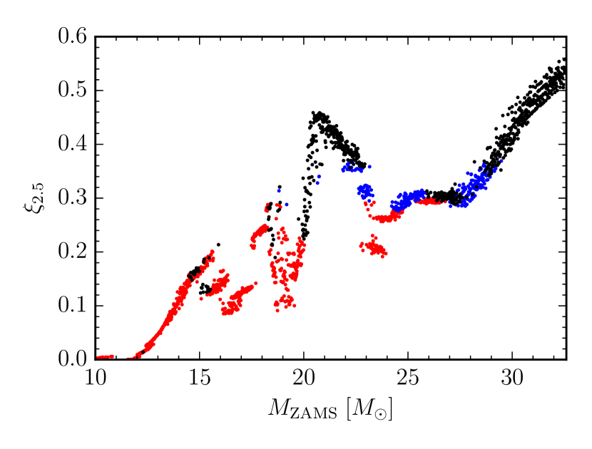
Figure 6: Compactness parameters $\xi_{2.5}$ for exploding (red) and non-exploding (black) models as a function of ZAMS mass. Blue dots denote models where shock revival is initiated, but the explosion eventually fails because the diagnostic energy becomes negative as the shock propagates out or the neutron star mass exceeds the maximum neutron star mass due to ongoing accretion in the explosion phase.

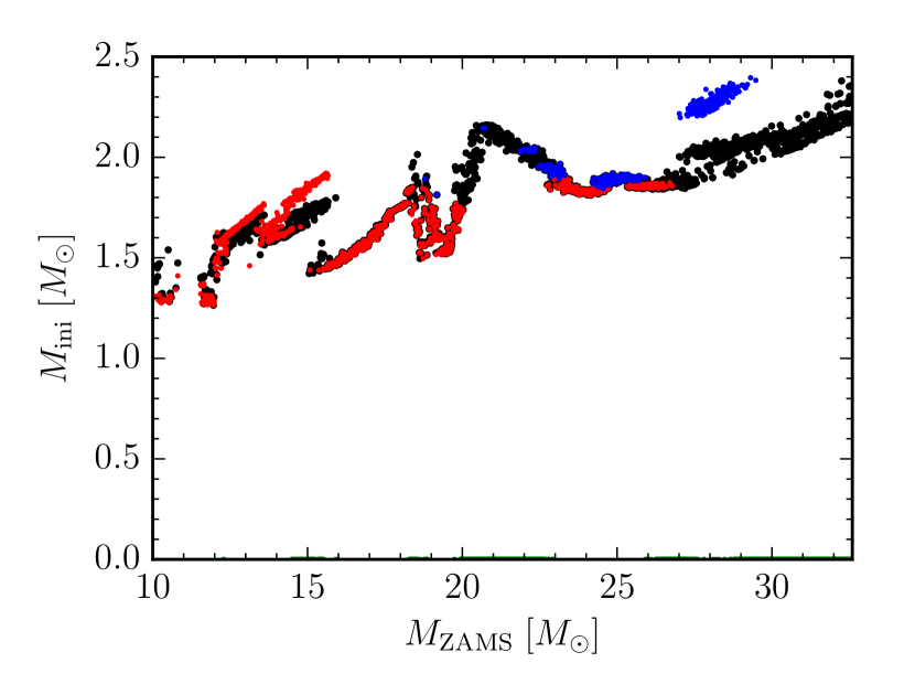
Figure 7: Mass coordinate $M_{\mathrm{ini}}$ of the initial mass cut as a function of ZAMS mass (red/blue dots). Red dots denote models that explode successfully, while blue dots are used for models where we predict black hole formation due to continued accretion after shock revival. The mass of the silicon core is shown in black.

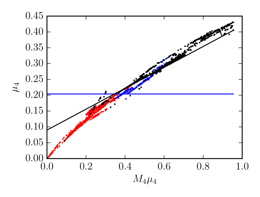
Figure 8: Distribution of the progenitor models in the $M_{4}\mu_{4}$-$\mu_{4}$ plane introduced by Ertl et al. (2016). Cases of neutron star formation, black hole formation without shock revival and black hole formation after shock revival are shown as red, black, and blue dots, respectively. Exploding and non-exploding can be reasonably well separated by $\mu_{4}=0.203$ (black line). A better discrimination between explosions and failures using an Ertl-type line $\mu_{4}=k_{1}\mu_{4}M_{4}+k_{2}$ with positive slope is precluded by the location of models that form black holes after shock revival due to continued accretion. Models with and without shock revival are nicely distinguished by a modified Ertl criterion $\mu_{4}=0.33\mu_{4}M_{4}+0.09$ with only 133 false identifications.

3.2 Comparison to Proposed Explosion Criteria

The qualitative similarity of the regions of neutron star and black hole formation with approaches that rely on 1D hydrodynamics simulations (O’Connor & Ott, 2011; Ugliano et al., 2012; Ertl et al., 2016; Sukhbold et al., 2016) is reassuring as these models arguably treat the phase up to shock revival more accurately than our analytic model in Section 2.1. The fundamental agreement about the conditions for shock revival (as opposed to the explosion and remnant properties in case of successful explosion that we discuss in Section 3.3) is borne out by an analysis of several phenomenological explosion criteria that have been proposed on the basis of 1D models.

3.2.1 Compactness Parameter

O’Connor & Ott (2011) introduced the compactness parameter $\xi_{M}$, which is defined for a given mass coordinate $M$ as

$$\xi_{M}=\frac{M/M_{\odot}}{r(M)/1000\,\mathrm{km}},$$ (51)

where $r(M)$ is the radial coordinate of this mass shell at the time of core bounce. They suggested $\xi_{2.5}\lesssim 0.45$ as a rough condition for successful explosions Subsequently, the parameterised 1D study of Ugliano et al. (2012) revealed a broad transition region between neutron star and black hole formation in the range $\xi_{2.5}\approx 0.15\ldots 0.35$. The distribution of the compactness parameters for our exploding and non-exploding models is shown in Figure 6. In line with the weaker tendency for black hole formation around $15\,M_{\odot}$, the transition region between neutron star and black hole formation is located at somewhat higher values than in Ugliano et al. (2012), i.e., $\xi_{2.5}=0.2\ldots 0.4$ with some outliers of black hole formation at even lower $\xi_{2.5}$. A choice of $\xi_{2.5,\mathrm{crit}}=0.278$ for the critical value best discriminates between explosions and non-explosions (with 158 false identification).

3.2.2 Ertl Criterion

While $\xi_{2.5}$ has been justified empirically as a measure of “explodability”, it evidently provides no sharp dividing line between explosion and failure, and aside from a vague connection with the maximum neutron star mass it lacks an intuitive theoretical basis. Ertl et al. (2016) therefore proposed a different criterion with higher discriminating power which is based on the structure of the progenitor near the outer edge of the Si core, whose infall typically results in a considerable improvement in heating conditions and is often closely associated with the transition to explosion in 1D (Ugliano et al., 2012; Ertl et al., 2016) and self-consistent multi-D simulations (Buras et al., 2006; Marek & Janka, 2009; Müller et al., 2012a; Suwa et al., 2016). They considered the two parameters $M_{4}$, the mass coordinate corresponding to an entropy of $s=4\ k_{\mathrm{b}}/\mathrm{nucleon}$ (which typically defines the interface between the Si core and the O shell), and $\mu_{4}$,

$$\mu_{4}=\frac{0.3}{[r(M_{4}+0.3\,M_{\odot})-r(s=4)]/1000\,\mathrm{km}}\propto\left.\frac{\mathrm{d}M}{\mathrm{d}r}\right|_{s=4},$$ (52)

which can be related to the accretion rate $\dot{M}\propto\mu_{4}$ and the accretion luminosity $L_{\mathrm{acc}}\propto\mu_{4}M_{4}$ shortly after the infall of the Si/O interface. Ertl et al. (2016) further argue that a calibrated linear inequality

$$\mu_{4}<k_{1}\mu_{4}M_{4}+k_{2},$$ (53)

can then be used to decide whether the critical neutrino luminosity for explosion (Burrows & Goshy, 1993) is reached or exceeded around the infall of the shell interface so that it can be used as a predictor for shock revival (provided that the heating conditions do not improve significantly later on). Since $\mu_{4}$ and $\mu_{4}M_{4}$ are loosely correlated with the accretion rate and the accretion luminosity around the infall of the Si/O interface, one expects the coefficient $k_{1}$ to be positive to reflect the monotonic increase of the critical luminosity with $\dot{M}$.

While it has more of a physical justification than the compactness parameter, the Ertl parameter rests on two important assumptions: It presupposes that successful shock revival generally also leads to a successful explosions, which is by no means to be taken for granted considering that some long-time multi-D supernova models show continued accretion over seconds (Müller, 2015), which implies that many progenitor could undergo delayed black hole formation even after successful shock revival. Furthermore, in some multi-D simulations (Marek & Janka, 2009; Müller et al., 2012a; Melson et al., 2015b; Lentz et al., 2015), shock revival is delayed considerably beyond the infall of the Si/O interface and is instead triggered by a continuing improvement of the heating conditions due to the increase of the mean energy with neutron star mass (cp. Müller & Janka, 2015).

Our model allows for both of these scenarios, and they are in fact realised in the standard case as demonstrated by Figure 7, which compares the mass coordinate $M_{\mathrm{ini}}$ for which we predict shock revival with the mass of the iron and Si core. Although shock revival generally occurs at or shortly outside the Si/O interface, there are progenitors with considerable delays between $27\,M_{\odot}$ and $30\,M_{\odot}$. Most of these, as well as some cases at slightly smaller ZAMS masses undergo delayed black hole formation after shock revival.

This turns out to be somewhat problematic for formulating an optimal Ertl criterion because the cases of late black hole formation tend to lie at higher $\mu_{4}M_{4}$ for a given $M_{4}$, i.e., one would expect the ratio of accretion luminosity to critical luminosity to be higher for these after the infall of the Si/O interface. We illustrate this in Figure 8, which shows the distribution of our progenitors in the $\mu_{4}M_{4}$-$\mu_{4}$ plane. For an optimal discrimination between exploding and non-exploding cases, we are forced to resort to an extreme choice $k_{1}=0$ for the slope, so that the Ertl criterion again becomes a one-parameter criterion,

$$\mu_{4}\lesssim 0.204.$$ (54)

This still furnishes a relatively good dividing line between exploding and non-exploding progenitors, but counterintuitively with a few more false predictions (188) than the compactness parameter. As a predictor for shock revival alone, the Ertl criterion fares considerably better, with just 133 ($6.3\%$) false predictions with the modified criterion

$$\mu_{4}=0.33\mu_{4}M_{4}+0.09.$$ (55)

Our results can of course not be taken as a test or a comparison of these criteria, since they are based on a very simplified model themselves. The numbers of false identifications mostly provide a consistency check between different approaches, and at best help to bolster these phenomenological criteria under different physical assumptions for the energetics and dynamics of the explosion phase: Despite the complications introduced by accretion after shock revival, both the compactness parameter and the Ertl criterion can still be relied upon for rule-of-thumb estimates for explodability. False positives and false negative never lie far away from the dividing line, and it is doubtful whether a reliable calibration of these criteria using multi-D or even only 1D simulations is possible at the present state of supernova theory. If different criteria and models agree for $90\%$ of all progenitor models, this rather points to a high level of compatibility.

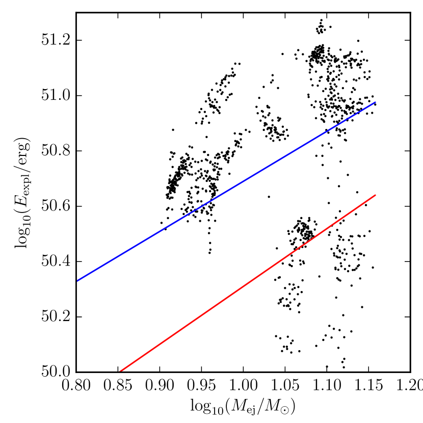
Figure 9: Plot of explosion energy $E_{\mathrm{expl}}$ versus ejecta mass $M_{\mathrm{ej}}$ for successfully exploding models. Fitted power laws for observed supernovae from Pejcha & Prieto (2015) using two different calibrations of their light curve model based on Litvinova & Nadezhin (1985) and Popov (1993) are shown in red and blue, respectively. While the bulk of our progenitor models conform to the observed correlation between $E_{\mathrm{expl}}$ versus ejecta mass $M_{\mathrm{ej}}$, there is also a sub-population of underenergetic supernovae from high-mass progenitors. This sub-population would likely exhibit considerable fallback, which could bring it back in line with the general trend.

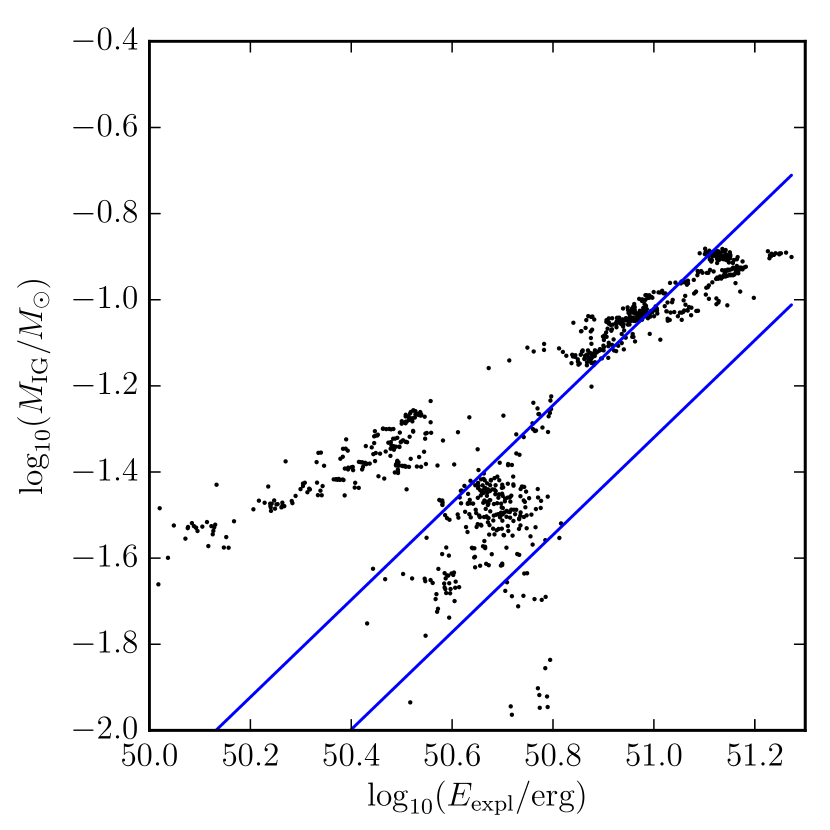
Figure 10: Explosion energy $E_{\mathrm{expl}}$ versus iron group mass $M_{\mathrm{IG}}$. A fitted power law for the dependence of $E_{\mathrm{expl}}$ on the nickel mass $M_{\mathrm{Ni}}$ for observed supernovae from Pejcha & Prieto (2015) using their light curve model calibrated against Popov (1993) is shown in blue (lower line). The upper blue line corresponds to twice the value of the fit of Pejcha & Prieto (2015) and roughly defines a band where $M_{\mathrm{IG}}$ is expected to lie considering that nickel will only make up part of the iron group elements produced by explosive burning.

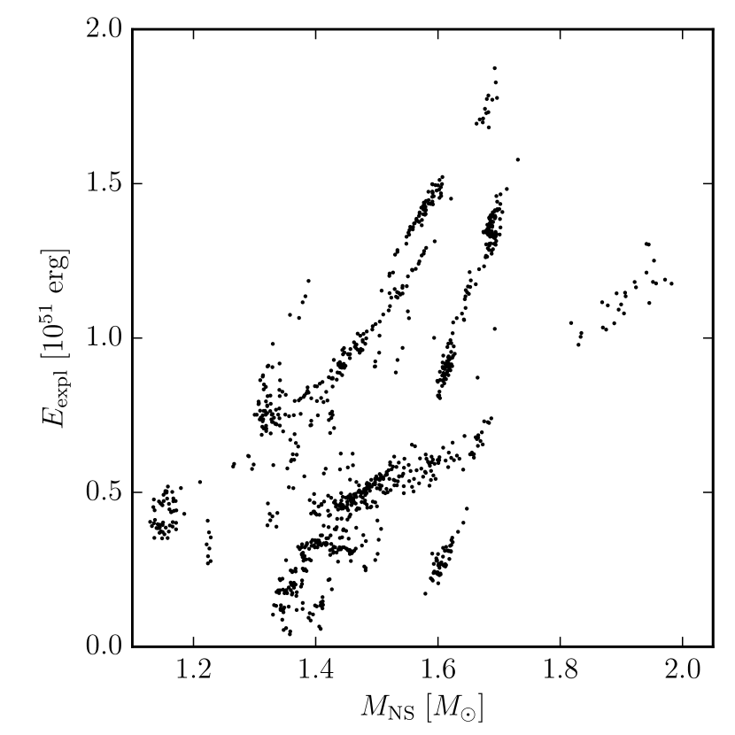
Figure 11: Explosion energy versus gravitational neutron star mass for successful explosions. Typically, more energetic explosions also tend to produce more massive neutron stars, but there is considerable scatter. Moreover, our model yields, perhaps spuriously, a clump of high-mass neutron stars from supernovae with moderate explosion energy.

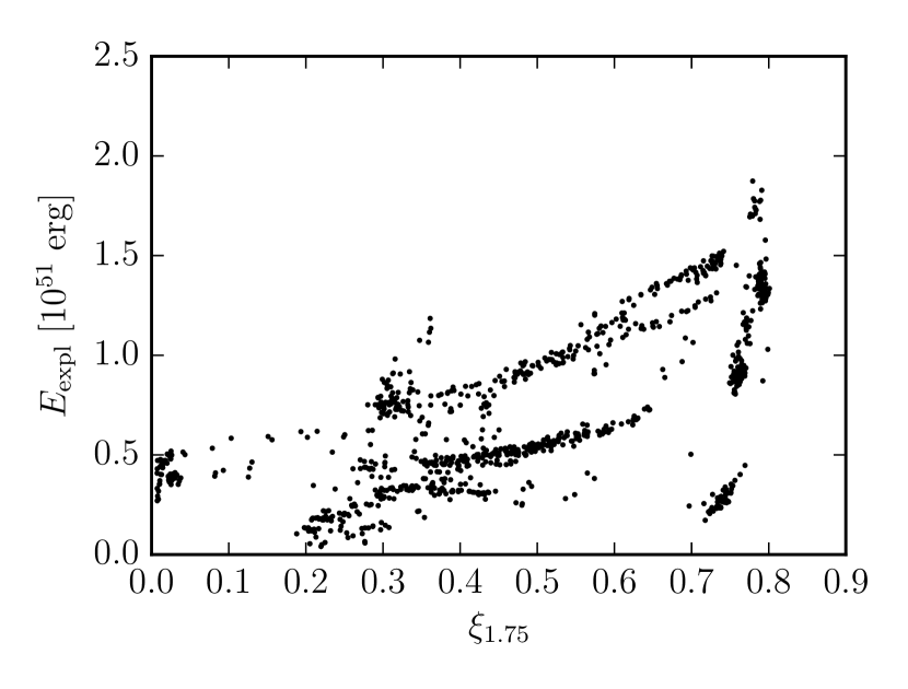
Figure 12: Explosion energy versus $\xi_{1.75}$. Highly energetic explosions only come from progenitors with large $\xi_{1.75}$, but aside form this there is no tight correlation between $\xi_{1.75}$ and $E_{\mathrm{expl}}$.

3.3 Explosion and Remnant Properties – Standard Case

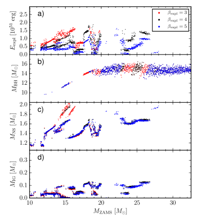
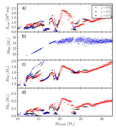
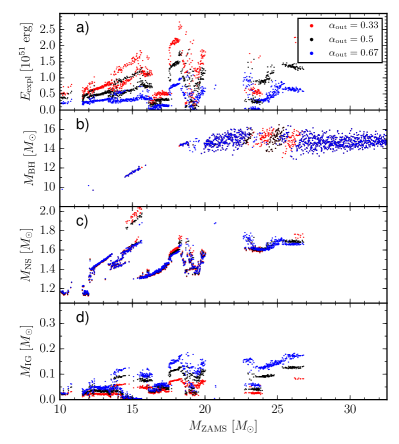
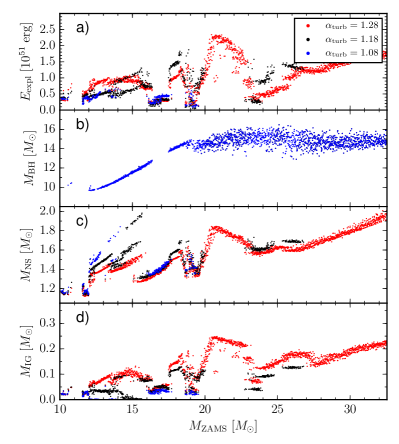
Figure 13: Dependence of the landscape of explosion energies $E_{\mathrm{expl}}$ (sub-panel a), gravitational remnant masses for black holes ($M_{\mathrm{BH}}$, sub-panel b) and neutron stars ($M_{\mathrm{NS}}$, sub-panel c), and iron-group masses (sub-panel d) $M_{\mathrm{IG}}$ on the shock compression ratio $\beta_{\mathrm{expl}}$ (top left), the efficiency factor $\zeta$ for the accretion luminosity (top right), the outflow surface fraction $\alpha_{\mathrm{out}}$ (bottom left), and the factor $\alpha_{\mathrm{turb}}$ for additional shock expansion due to higher turbulent pressure (bottom right).

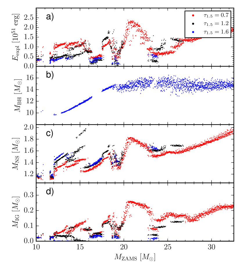
Figure 14: Dependence of the landscape of explosion energies $E_{\mathrm{expl}}$ (panel a), gravitational remnant masses for black holes ($M_{\mathrm{BH}}$, sub-panel b) and neutron stars ($M_{\mathrm{NS}}$, sub-panel c), and iron-group masses $M_{\mathrm{IG}}$ (panel d) on the cooling time-scale $\tau_{\mathrm{1.5}}$ for a $1.5\,M_{\odot}$ neutron star.

While our model thus agrees well with the literature when it comes to predicting the explodability of supernova progenitors, we see pronounced differences to Ugliano et al. (2012) and Pejcha & Thompson (2015) in the landscape of explosion and remnant properties.

3.3.1 Remnant Mass Distribution

One of the conspicuous features of our model is the prediction of a multi-modal distribution of neutron star masses (Figure 3) with peaks around $1.15\,M_{\odot}$, and $1.45\,M_{\odot}$, and possibly a third one at $1.9\,M_{\odot}$ which is qualitatively similar to Zhang et al. (2008) and case a) of Pejcha & Thompson (2015), but more conspicuous than in the work of Ugliano et al. (2012). The emergence of prominent peaks at low neutron star masses may simply be due to the better sampling of small ZAMS masses in our larger set of progenitors, and the susceptibility of explosions from these progenitors to fallback due to their extended hydrogen envelope (Ugliano et al., 2012) could eventually change the peak structure somewhat. The location of the peaks is somewhat different from the bimodal distribution of neutron stars inferred by Schwab et al. (2010) with peaks at $1.25\,M_{\odot}$ and $1.35\,M_{\odot}$, and is pushing the limits of the observed neutron star mass distribution at low masses $\mathord{\lesssim}1.2\,M_{\odot}$, where we find a far more prominent peak than measured neutron star masses (Lattimer, 2012) would suggest. Possible reasons and remedies for this discrepancy will be discussed later.

Nonetheless, it is noteworthy that a bi- or multi-modal neutron star mass distribution can naturally be obtained without invoking a separate stellar evolution channel such as electron capture supernovae, which have been proposed as the origin of neutron stars around $1.25\,M_{\odot}$ (Schwab et al., 2010). Structural variations towards the low-mass end of the iron-core supernova progenitor population alone might provide an explanation for the observed mass distribution. At the same time, there is a sufficiently extended tail of the distribution to produce neutron stars with birth masses $>1.7\,M_{\odot}$ mostly from stars between $15\,M_{\odot}$ and $20\,M_{\odot}$. Such high birth masses are required to account for cases like the Demorest pulsar, whose birth mass must have been at least $1.7\,M_{\odot}$ (Tauris et al., 2011),

We note, however, that the location of the peaks is somewhat different to those postulated by Schwab et al. (2010) whose inferred distribution of spin-corrected masses (from 14 well-measured cases) peaks at $1.25\,M_{\odot}$ and $1.35\,M_{\odot}$ with an additional outlier at $1.6\,M_{\odot}$. There is a number of possible reasons for such a discrepancy; it could point to an overestimation of the Fe and Si core size in stellar evolution models or a bias in the measured masses due to binary evolution effects. It could also imply that shock revival needs to be triggered earlier, i.e., already in the Si shell. Since the neutron excess in the Si shell dramatically affects the yields during explosive burning, this is only a viable scenario for a subset of core-collapse supernovae with supersolar Ni/Fe ratios in the ejecta (Jerkstrand et al., 2015) and could not provide a general path towards smaller neutron star masses due to nucleosynthesis constraints on the neutron excess in ejecta processed by explosive burning (Woosley et al., 1973).

3.3.2 Systematics of Explosion Energies and Nickel Masses

While previous approaches to predict the landscape of supernova explosion energies using parameterised models have all obtained (by construction) a similar range for $E_{\mathrm{expl}}$, some of them are diametrically opposed concerning the dependence of $E_{\mathrm{expl}}$ on the ZAMS mass. Ugliano et al. (2012) and Pejcha & Thompson (2015) have obtained powerful explosions for low-mass progenitors, and in the case of Pejcha & Thompson (2015), there is even an extreme negative correlation between ZAMS mass and explosion energy. This is due to the major role of the neutrino-driven wind in powering the explosion in these studies, which hinged on the neutron star cooling model in the case of Ugliano et al. (2012) and an overly optimistic analytic estimate for the wind power in Pejcha & Thompson (2015). High explosion energies for low-mass progenitors are, however, inconsistent both with simulations that point to explosion energies of only a few $10^{50}\,\mathrm{erg}$ for low-mass supernovae (Buras et al., 2006; Bruenn et al., 2016; Melson et al., 2015a; Müller, 2015). Although multi-D simulations are still limited in their ability to scan the parameter space systematically, they rather point towards a positive correlation between ejecta mass and explosion energy (Bruenn et al., 2016; Nakamura et al., 2015), as does the observational evidence (Poznanski, 2013; Chugai & Utrobin, 2014; Pejcha & Prieto, 2015).

Among the extant parameterised models, such a positive correlation has been found by Perego et al. (2015), below ZAMS masses of $15\,M_{\odot}$ by Ertl et al. (2016), and below $13\,M_{\odot}$ by Sukhbold et al. (2016). Perego et al. (2015) relied on a rather ad hoc prescription for boosting the neutrino heating in a pre-specified time interval, however, and only explored a narrow mass window between $18\,M_{\odot}$ and $21\,M_{\odot}$ in ZAMS mass. Similarly, Ertl et al. (2016) introduced a modification of their core cooling model to suppress the core luminosity depending on $\xi_{1.75}$, which is prompted by an analysis of the shortcomings of the initial cooling model of Ugliano et al. (2012), but still savours of a somewhat arbitrary solution, especially since a parameter characterising a single mass shell in the progenitor is used to control the diffusion luminosity from the core at all times. Sukhbold et al. (2016) find a correlation between $M_{\mathrm{ZAMS}}$ and $E_{\mathrm{expl}}$, but only in a very restricted mass range. They provide some physical motivation for a slightly different modification of the cooling model, but this comes at the expense of using different contraction laws for the inner boundary of the grid and in the cooling model. Moreover, the parameters of the cooling law are still chosen a priori based on the mass enclosed in the the innermost $3000\,\mathrm{km}$ in the progenitor, and an additional “Crab-like” calibration model at the lower mass end is needed, so, in a sense, the expected result is still put in by hand.

Figure 2 already suggests that our model is well in line with the observed correlations without the need for excessive tweaking. At the low-mass end, we obtain explosion energies as low as $2.6\times 10^{50}\,\mathrm{erg}$, whereas all of the energetic explosion with energies $>10^{51}\,\mathrm{erg}$ occur at higher ZAMS masses, especially in the islands of explodability around $18\,M_{\odot}$ and $22\,M_{\odot}\ldots 25\,M_{\odot}$. There is, however, a subset of low-energy explosions at high masses. These are cases on the borderline between neutron star and black hole formation, where the energy input by neutrinos and nucleon recombination barely outweighs the binding energy of the envelope. We shall critically examine this sub-population in more detail below.

In Figure 9, we compare the distribution of ejecta masses $M_{\mathrm{ej}}$ and explosion energies $E_{\mathrm{expl}}$ with fitted power laws for observed core-collapse events derived by Pejcha & Prieto (2015) for two different calibrations of their model for light curves and expansion velocities. With a calibration based on Litvinova & Nadezhin (1985), they find

$$\log(E_{\mathrm{expl}}/10^{50}\,\mathrm{erg})=2.09\log(M_{\mathrm{ej}}/M_{\odot})-1.78,$$ (56)

while calibrating against (Popov, 1993) yields

$$\log(E_{\mathrm{expl}}/10^{50}\,\mathrm{erg})=1.81\log(M_{\mathrm{ej}}/M_{\odot})-1.12\;.$$ (57)

The bulk of the models fit the power law (56) reasonably well, although our predicted energies are slightly higher. Equation (56) suggests very small explosion energies; even for the maximum ejecta mass theoretically allowed by our progenitor models, one would obtain energies only up to $\mathord{\approx}4\times 10^{50}\,\mathrm{erg}$. This simply reflects calibration problems in the observational determination of supernova explosion properties. Given these discrepancies between different approaches for determining explosion energies from light curves, the slope of the power laws is arguably to be trusted more than their normalisation. If we bear this in mind, the majority of our models are nicely in line with the observed correlation between $E_{\mathrm{expl}}$ and $M_{\mathrm{ej}}$.

The picture is similar for the nickel mass and its correlation to the explosion energy that has already been noted by Hamuy (2003). In Figure 10, we plot the distribution of our explosion models in the $E_{\mathrm{expl}}$-$M_{\mathrm{IG}}$ plane and compare with the empirical fit obtained by Pejcha & Prieto (2015) using Popov (1993) for calibration,

$$\log(M_{\mathrm{Ni}}/M_{\odot})=1.13\log(E_{\mathrm{expl}}/10^{50}\,\mathrm{erg})-2.45.$$ (58)

Except for the subset of low-energy explosions from high ZAMS masses clustering around $17\,M_{\odot}$, $19\,M_{\odot}$ and $24\,M_{\odot}$, our model typically predicts iron group masses that agree with the fitted power law within a factor of two.

The low-energy explosions at high masses are still worrisome. We surmise that for these cases the predictions of our model become rather shaky because one expects considerable fallback. This would imply that the observed explosion energy (carried by the ejecta that avoid fallback) could well be higher, while $M_{\mathrm{ej}}$ and $M_{\mathrm{IG}}$ would be reduced, bringing the models back to the main branch that fits the power-law dependence of $E_{\mathrm{expl}}$ on $M_{\mathrm{ej}}$. Moreover, Figures 9 and 10 do not provide an adequate picture of the expected population of observed supernovae: Even if we take the prediction of such low-energy explosions with high ejecta mass seriously, these events would be rare because of the steep slope of the IMF, and they would be faint since the plateau luminosity scales as $L_{\mathrm{SN}}\propto E_{\mathrm{expl}}^{5/6}M_{\mathrm{ej}}^{-1/2}$ (Popov, 1993; Kasen & Woosley, 2009).

In stark contrast to Pejcha & Thompson (2015), and in qualitative agreement with Perego et al. (2015) and Nakamura et al. (2015), we find a positive correlation between neutron star mass and explosion energy (Figure 11), at least for the vast majority of progenitors. Again, the high-mass progenitors with low or moderate explosion energies on the borderline to black hole formation do not conform to the general trend; they are the origin of the cluster around $M_{\mathrm{NS}}=1.5\,M_{\odot}$ and $E_{\mathrm{expl}}=5\times 10^{50}\,\mathrm{erg}$ and lower. There are also outliers at $M_{\mathrm{NS}}\gtrsim 1.8\,M_{\odot}$ and $E_{\mathrm{expl}}\approx 10^{51}\,\mathrm{erg}$. Moreover, the scatter in the relation between $M_{\mathrm{NS}}$ and $E_{\mathrm{expl}}$ is huge. It is even more pronounced if we plot $E_{\mathrm{expl}}$ against the compactness parameter $\xi_{1.75}$ (see Figure 12), the parameter considered as a correlate to the explosion energy by Perego et al. (2015). We only find a tendency for very energetic explosions to occur only at high $\xi_{1.75}$, but no tight correlation. This is to be expected because the final explosion energy is essentially a difference of two quantities that can be of similar magnitude, i.e., the energy release by nucleon recombination and nuclear burning and the binding energy of the progenitor. While either of these will correlate with the proto-neutron star mass, which directly and indirectly (through correlations with the structure of the O shell) influences the critical radius where accretion ceases and hence the amount of material accreted during the explosion phase, the difference between them will strongly correlate with the proto-neutron star mass, the mass of the Si core, or the compactness parameter only over limited ranges of ZAMS mass, where the structure of the progenitor remains quasi-homologous. Resorting to single parameters like $\xi$, $M_{4}$, or $\mu_{4}M_{4}$ as predictors for the explosion energy therefore seems a somewhat more dubious than using them as predictors for shock revival only.

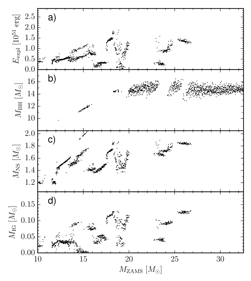
Figure 15: Explosion energy $E_{\mathrm{expl}}$ (panel a), gravitational remnant mass for black holes ($M_{\mathrm{BH}}$, sub-panel b) and neutron stars ($M_{\mathrm{NS}}$, sub-panel c), and the iron-group mass $M_{\mathrm{IG}}$ (panel d) as a function of ZAMS mass for the standard set of parameters, but assuming that mass accreted onto the neutron star is not partially re-ejected (Equation 59). Note that there is a gap in our set of progenitors around $11\,M_{\odot}$; missing data points in this region are not indicative of black hole formation.

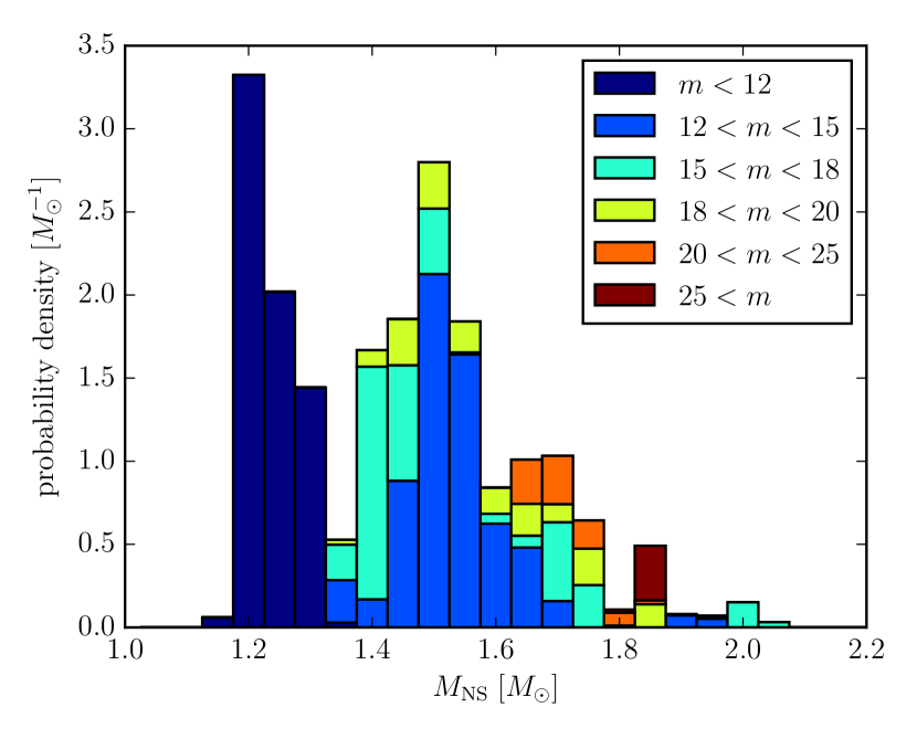
Figure 16: Histogram of the distribution of gravitational neutron star masses for for the standard set of parameters, but assuming that mass accreted onto the neutron star is not re-ejected (Equation 59) . The stacked bars in different colours give the contribution of progenitors from different ranges of the ZAMS mass $m$ (measured in solar masses) to the average probability density in a given bin.

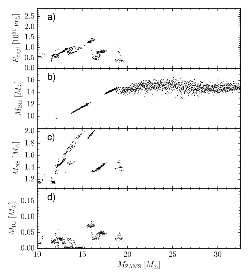
Figure 17: Explosion energy $E_{\mathrm{expl}}$ (panel a), gravitational remnant mass for black holes ($M_{\mathrm{BH}}$, sub-panel b) and neutron stars ($M_{\mathrm{NS}}$, sub-panel c), and the iron-group mass $M_{\mathrm{IG}}$ (panel d) as a function of ZAMS mass for $\alpha_{\mathrm{turb}}=1.15$ and $\beta_{\mathrm{expl}}=3$. For this choice of parameters, most progenitors above $\gtrsim 18\,M_{\odot}$ form black holes.

3.4 Sensitivity to Model Parameters

The qualitative agreement of our model with some of the observational constraints (leaving aside the subset of low-energy explosions from high-mass stars) is encouraging, but does it actually mean that the physics of the neutrino-driven explosion mechanism accounts for the observational trends, or is this just a “lucky shot”? What physical ingredients in the model need to be changed to iron out the remaining tensions with the observational evidence?

This is a critical question for any parameterised approach to the progenitor-explosion connection, also for calibrated ones that reproduce the explosion properties of one or a few cases by construction (Ugliano et al., 2012; Ertl et al., 2016; Sukhbold et al., 2016). So far, only Pejcha & Thompson (2015) have attempted to assess the robustness of their predictions in a systematic way. Our model has a considerable advantage in that it allows us to test the impact of variations in physical parameters that characterise physical process in the supernova core (such as the efficiency of the conversion of accretion energy into luminosity) rather than abstract exponents in a power law for the critical luminosity as in Pejcha & Thompson (2015).

To assess the sensitivity of our results to the model parameters, we primarily consider variations of single parameters around their standard values. The resulting distribution of the explosion parameters for variations in $\beta_{\mathrm{expl}}$, $\zeta$, $\alpha_{\mathrm{out}}$, $\alpha_{\mathrm{turb}}$, and $\tau_{\mathrm{1.5}}$ are shown in Figures 13 and 14.

Broadly speaking, the model parameters can be divided into two classes: $\beta_{\mathrm{expl}}$ and $\alpha_{\mathrm{out}}$, primarily influence $E_{\mathrm{expl}}$, $M_{\mathrm{NS}}$, and $M_{\mathrm{IG}}$ for exploding models but affect the regions of black hole and neutron star formation only to a minor degree. $\alpha_{\mathrm{turb}}$, $\zeta$, and $\tau_{\mathrm{1.5}}$ have a larger impact on success and failure.

3.4.1 Sensitivity to Accretion After Shock Revival

Increasing $\beta_{\mathrm{expl}}$ or decreasing $\alpha_{\mathrm{out}}$ results in higher explosion energies because this allows a larger amount of mass to be accreted onto the neutron star and drive an outflow in the process. The overall dependence of $E_{\mathrm{expl}}$ on ZAMS mass stays rather similar; in most regions the effect is tantamount to a mere rescaling of the explosion energy. Too much additional accretion onto the neutron star leads to black hole formation, however, so that the island of explodability around $23\,M_{\odot}$ disappears for $\beta_{\mathrm{expl}}=3$, for example. It is noteworthy that the distribution of neutron star masses is only considerably affected for extreme choices of $\beta_{\mathrm{expl}}$. This is due to our assumption that a fraction $\eta_{\mathrm{acc}}/|e_{\mathrm{g}}|$ of the accreted material is re-channelled into an outflow (Equation 48), which allows the cycle of accretion, neutrino heating, and mass ejection to run without a strong growth of the neutron star mass if this fraction is high. Considering the overall uncertainties in the model, $\eta_{\mathrm{acc}}/|e_{\mathrm{g}}|$ may well be overestimated, which would imply a stronger sensitivity of $M_{\mathrm{NS}}$ to $\beta_{\mathrm{expl}}$ and $\alpha_{\mathrm{turb}}$ and could shift its distribution to higher masses. Even if we neglect re-ejection completely in the mass budget and replace Equation (48) with

$$\frac{dM_{\mathrm{by}}}{dM_{\mathrm{sh}}}=1-\alpha_{\mathrm{out}}\;,$$ (59)

however, this does not affect the landscape of explosion properties qualitatively (Figure 15). Essentially, the effect amounts to an upward shift of the peaks of the distribution by $0.05\,M_{\odot}$ to $1.2\,M_{\odot}$ and $1.5\,M_{\odot}$ (Figure 16). This would bring the low-mass peak more in line with observations, but increase the tension between the predictions and the observed neutron star mass distribution (Lattimer, 2012; Schwab et al., 2010) at the high-mass end.

The amount of iron group elements $M_{\mathrm{IG}}$ produced by explosive burning is little affected by increasing $\beta_{\mathrm{expl}}$, on the other hand, because longer accretion does not increase the shock velocity and post-shock temperature at early times to allow for explosive burning to the iron group in a more extended layer. $M_{\mathrm{IG}}$ also (understandably) decreases for lower $\alpha_{\mathrm{out}}$, as a smaller fraction of the burnt material is swept along with the ejecta. This implies that one can only trust and expect agreement to empirical correlations between $E_{\mathrm{expl}}$ and $M_{\mathrm{IG}}$ like Equation (58) as far as the power-law index is concerned since the distribution of these two quantities can easily be rescaled in different directions within our model.

The shape of the distribution of explosion energies and nickel masses as a function of ZAMS mass emerges as a relatively robust feature, however. This is an encouraging result and suggests that the neutrino-driven mechanism can provide a viable explanation for the observed correlations between $E_{\mathrm{expl}}$, $M_{\mathrm{ej}}$ and $M_{\mathrm{Ni}}$.

3.4.2 Sensitivity of Shock Revival to Model Parameters

$\zeta$, $\tau_{1.5}$, and $\alpha_{\mathrm{turb}}$ also affect the heating conditions prior to shock revival, and can change the regions of neutron star and black hole formation considerably. The relatively weak tendency towards black hole formation around $15\,M_{\odot}$ compared to Ugliano et al. (2012) in the standard case is therefore not indicative of a fundamental disagreement. It merely reflects the strong sensitivity of shock revival or failure to the assumed physics, which is perfectly in line with the mixed record of multi-D simulations, and which also surfaced, albeit to a smaller degree, in the exploration of different calibration models in Ertl et al. (2016) and Sukhbold et al. (2016). Given this sensitivity, current parameterised models can arguably be trusted only to the extent that they predict a tendency towards black hole and neutron star formation for certain intervals in ZAMS mass, but their extent should be taken as rather uncertain. Our result suggests that theoretical models are in principle compatible with observational evidence that no massive stars above $\mathord{\approx}18\,M_{\odot}$ explode as Type IIP supernovae (Smartt, 2015) if we disregard other constraints on explosion energies and nickel masses for the time being.

Generally (but not invariably), choices for $\zeta$, $\tau_{1.5}$, and $\alpha_{\mathrm{turb}}$ that give a large fraction of explosions also results in higher explosion energies and iron group masses, and smaller neutron star masses overall. This implies that one needs to adjust $\beta_{\mathrm{expl}}$ or $\alpha_{\mathrm{out}}$ if the overall fraction of successful explosions goes down in order to obtain reasonable explosion energies. This is possible for plausible combinations of parameters, e.g., for $\alpha_{\mathrm{turb}}=1.15$ and $\beta_{\mathrm{expl}}=3$, which gives a low upper mass limit for successful explosions in line with Smartt (2015) as shown by Figure 17, but unavoidably results in a more prominent high-mass tail in the distribution of neutron star masses, which is somewhat at odds with the inferred birth mass distribution (Schwab et al., 2010) in binary systems.

Figures 13 and 14 also illustrate that better heating conditions during the accretion phase due to higher $\alpha_{\mathrm{turb}}$ and $\zeta$ or smaller $\tau_{1.5}$ can easily result in a landscape of explosion energies that appears unrealistic not only because of a complete lack of black hole formation cases, but because of a high incidence of high nickel/iron group masses among the entire population of core-collapse supernovae. Moreover, increasing the heating conditions by shortening the cooling time-scale $\tau_{1.5}$ tends to destroy the correlation between ejecta mass and explosion energy for progenitors below $20\,M_{\odot}$. This could be a problem for scenarios for more efficient shock revival that rely on a faster release of the thermal energy of the proto-neutron star core, such as active-sterile neutrino conversion and re-conversion (Hidaka & Fuller, 2007).

3.4.3 Implicitly Fixed Parameters

The reader should bear in mind that our model still contains a few parameters other than $\beta_{\mathrm{expl}}$, $\zeta$, $\alpha_{\mathrm{out}}$, $\alpha_{\mathrm{turb}}$, and $\tau_{\mathrm{1.5}}$, which we have implicitly considered as fixed because they are arguably not as uncertain as the other ones, or because changing them would largely amount to a rescaling of some other parameter. For these reasons, variations in these parameters do not warrant an extended discussion, and we do not provide plots to illustrate them. We nevertheless briefly comment in a non-exhaustive fashion on the resulting effects for a few selected parameters. Shortening the infall time by using a different coefficient in Equation (2) generally delays shock revival and leads to more prevalent black hole formation. Increasing the fraction of electron neutrinos and antineutrinos in the diffusive flux in Equation (13) tends to increase the explosion fraction and make the explosions more energetic across the whole mass range. Increasing the effect of gravitational redshift on the neutrino luminosity (16) by computing it for a smaller radius $r_{\mathrm{PNS}}<5/7r_{\mathrm{g}}$ obviously decreases the explosion fraction, with a more pronounced effect for massive progenitors with large iron and silicon cores. Increasing the coefficient in Equation (35) for the shock velocity is largely tantamount to increasing $\beta$ and shortening the phase of accretion after shock revival (which generally decreases the final explosion energies). Increasing $\epsilon_{\mathrm{rec}}$ in Equation (37), i.e., the contribution of neutrino-heated ejecta to the explosion energy per unit mass, leads to an earlier termination of accretion and lower neutron star masses; the higher asymptotic energy of the ejecta largely balances the shorter duration of neutrino-driven mass ejection, so that explosion energies are not too strongly affected, especially for low progenitor masses. Iron group masses are obviously directly affected by the threshold temperature for silicon burning; but other than that the threshold temperatures for the different explosive burning processes have little effect on the other explosion parameters as long as explosion energy is primarily provided by neutrino heating.

Obviously, some of the independent parameter variations explored in this section would already result in a distribution of explosion energies and remnant properties that is in conflict with one or more observational constraints (range of observed explosion energies, explosion properties of SN 1987A, etc.). This could suggest that the allowed variations in the landscape of explosion properties are actually much smaller than this section might suggest, and that even their absolute values – and not only general trends and correlations – can be predicted with good accuracy with the help of one or two calibration cases. Without a more complete exploration of the high-dimensional parameter space this verdict ought to be left to the future.

4 Summary and Conclusions

In this paper, we set out to develop a theoretical approach to predict remnant and explosion properties of neutrino-driven core-collapse supernovae without an elaborate machinery of parameterised 1D neutrino-hydrodynamics simulations, let alone multi-D models. To this end, we constructed a simple model based on analytic approximations for the pre-explosion phase up to shock revival and simple ODEs in the explosion phase. For the first time, we attempt to take into account that continued accretion after shock revival plays a major role in powering the explosion. While we need to introduce a number of parameters, all of these have a physical motivation and significance, and multi-D simulations of supernova explosions can be used to calibrate them.

Our examination of the model predictions for an unprecedented number of 2120 progenitor models and their sensitivity to the model parameters are encouraging: Using plausible choices for physical parameters based on recent multi-D simulations, we can obtain a similar landscape of neutron star and black hole formation regions as time-dependent 1D models with neutrino transport (Ugliano et al., 2012; Ertl et al., 2016; Perego et al., 2015) or the hybrid approach of Pejcha & Thompson (2015) based partly on simulations and partly on analytic theory: For our standard set of parameters, there are some instances of black hole formation already at low ZAMS mass ($\approx 15\,M_{\odot}$), and some islands of explodability at high ZAMS mass. Good agreement with extant phenomenological explosion criteria like the progenitor compactness (O’Connor & Ott, 2011) and the Ertl criterion (Ertl et al., 2016) both validate our model and indicate that the inclusion of accretion after shock revival does not fundamentally affect predictions of the explodability of supernova progenitors.

By including a simple estimate for the duration of accretion after shock revival and the concomitant neutrino heating, we are able to reproduce observed correlations between the explosion energy and the ejecta mass (Poznanski, 2013; Chugai & Utrobin, 2014; Pejcha & Prieto, 2015) and between the explosion energy and the nickel mass (Hamuy, 2003; Pejcha & Prieto, 2015) naturally for the bulk of our progenitors. In agreement with the 2D study of Nakamura et al. (2015) and the parameterised 1D study of Perego et al. (2015) (which was restricted to progenitors between $18\,M_{\odot}$ and $21\,M_{\odot}$, however), we also find a loose correlation between neutron star mass and explosion energy, implying that the most energetic neutrino-driven explosions with $E_{\mathrm{expl}}\approx 2\times 10^{51}\,\mathrm{erg}$ leave behind neutron stars with masses $\gtrsim 1.7\,M_{\odot}$. For our standard case, we obtain a multi-modal neutron star mass distribution with peaks around $1.15\,M_{\odot}$, $1.45\,M_{\odot}$ and possibly $1.9\,M_{\odot}$. The low-mass peak emerges naturally from stars with ZAMS masses between $10\,M_{\odot}$ and $12\,M_{\odot}$.

An exploration of the sensitivity of our model predictions to individual parameters revealed that there is considerable leeway in parameterised approaches like ours to shift explosion energies and nickel masses up or down globally for the entire range of progenitor masses, but aside from that the functional dependence of $E_{\mathrm{expl}}$ and the produced amount of iron group elements on ZAMS mass appears rather robust. Similarly, plausible variations in the parameters can easily shift the peaks in the neutron star mass distribution by $\mathord{\gtrsim}0.05\,M_{\odot}$. Moreover, the overall fraction of neutron star and black hole formation can change considerably for reasonable parameter variations, indicating that empirical parameters for explodability, while useful as a rough metric, cannot provide a sharp dividing line between exploding and non-exploding models at the present state of supernova theory. In line with Clausen et al. (2015), we also find that the boundaries between regions of black hole and neutron star formation are fuzzy and both channels may be similarly prevalent in certain intervals of ZAMS mass so that a probabilistic description may be more adequate.

All this bodes well for one of the primary purposes of our model. On the level of accuracy and reliability that current parameterised 1D simulations have reached, it appears possible to estimate explosion properties of massive stars simply based on their structure without the relatively elaborate numerical machinery that approaches like Ugliano et al. (2012); Ertl et al. (2016); Perego et al. (2015) and Sukhbold et al. (2016) rely on. Our model, perhaps with some calibration against a specific reference case like SN 1987A as in Ugliano et al. (2012) or against other equally important constraints on the entire population of explosions, could provide input for systematic studies of supernova nucleosynthesis or for a quick exploration of the effect of new or uncertain physics in stellar evolution on supernovae from massive stars. Even without such a calibration, which always faces the dilemma of singling out the “best” and most important observational constraints, it is already useful for identifying trends and tendencies in the explosion properties and checking their robustness against parameter variations. It is remarkable and informative that a few relatively simple and physically motivated equations can capture the gist of more complicated simulations to a large degree. Obviously, this does not render parameterised 1D and 2D simulations obsolete, however. These are still superior in that they can treat many aspects of the supernova problem, among them the cooling and the contraction of the neutron star, explosive burning in the shock, and fallback (more) self-consistently, and can therefore potentially provide much firmer quantitative predictions for the observables discussed here: The range of parameter variations explored here may be allowed mathematically, but may not be realisable any more in a more rigorous approach.

Moreover, there are still some caveats and critical issues that will need to be re-examined in the future. Aside from some of the unavoidable oversimplifications and inconsistencies that come with analytic models, our approach still has two major shortcomings in terms of missing physics. Moreover, there are some tensions between observational constraints and the predictions not only of our model but also other parameteric studies in the literature.

The most obvious shortcoming that could account for some of these tensions is our all-our-nothing treatment of fallback due to the deceleration of material by the reverse shock (Chevalier, 1989). The recent results of Sukhbold et al. (2016), who found only few cases with more than $0.01\,M_{\odot}$ of fallback, suggest that there is little fallback for low-mass progenitors and for high-mass progenitors with rather high explosion energies. Thus, the distribution of neutron star masses (and even of nickel masses) may not be severely affected by fallback. We speculate, however, that considerable fallback could occur for our sub-population of low-energy explosions from high-mass stars, where the “initial” explosion energy and the binding energy of the envelope almost cancel. A more consistent treatment of fallback and the energy transfer from the inner ejecta to the envelope could help to eliminate this peculiar subset of explosions, or bring the inordinately high nickel and ejecta masses down to values that are in line with the observed systematics of core-collapse supernova explosions.

Moreover, the nickel (iron group) masses predicted by our very crude treatment of explosive burning should be taken with caution even though we can obtain a plausible range of values for most progenitors for appropriately chosen model parameters.

In the long run, more systematic multi-D studies of supernova explosions are needed to determine whether multi-D effects can be subsumed into a simple modification of the heating conditions in 1D prior to shock revival and a crude budget of mass inflow and outflow after shock revival. Many light-bulb based models of convection and the standing accretion shock instability (SASI) in supernova cores (Murphy & Burrows, 2008; Hanke et al., 2012), as well as the recent first-principle models of Summa et al. (2015) point in this direction, and there is also some theoretical justification for this (Müller & Janka, 2015). On the other hand, Cardall & Budiardja (2015) recently argued that the threshold for explosions is smeared out considerably in the SASI-dominated regime and subject to stochastic variations. Even if a simple rescaling of the 1D heating conditions were adequate in the SASI-dominated regime, the reduction in the required heating in 3D might be larger than for convection-dominated models (Fernández, 2015). For the explosion phase, the validity of simple phenomenological models is even less well explored so far. Finally, the (potentially crucial) role of multi-D seed asphericities from convective burning in shock revival (Couch & Ott, 2013; Müller & Janka, 2015; Couch et al., 2015) is not accounted for in our model at all.

In fact, additional physics like large seed perturbations for the hydrodynamic instabilities may be required to resolve the tensions between model predictions and observations: It appears rather difficult for parameterised models to produce a prominent second peak of the neutron star mass distribution at $1.35\,M_{\odot}$ as suggested by observations (Schwab et al., 2010), while at the same time covering a range of supernova energies up to $2\times 10^{51}\,\mathrm{erg}$. Could the (mild) discrepancy between predictions and observations be accounted for by selection effects in binaries, or by uncertainties in the core structure of massive stars, or does shock revival need to be initiated already in the Si shell for some models (Couch et al., 2015; Jerkstrand et al., 2015)? Alternatively, fallback in explosions of low-mass stars might merge the neutron star distribution into a single peak at the desired value of $1.35\,M_{\odot}$, and electron capture supernovae, which are not included here, could provide a separate peak at lower mass in line with the original idea of Schwab et al. (2010).

Similarly a cut-off for neutron star formation around $18\,M_{\odot}$ seems difficult to accommodate without either accepting small explosion energies or shifting the distribution of neutron stars up to higher gravitational masses. Could convective seed perturbations help to explode some progenitors energetically while not affecting most progenitors above $18\,M_{\odot}$? Or could uncertainties in the mass loss, or binary effects change the fate of progenitors above $18\,M_{\odot}$?

At present, any attempt to provide a coherent solution for these problems must remain highly speculative. Nonetheless, our improved understanding of the neutrino-driven mechanism has, despite some setbacks in simulations, clearly reached a stage where it can help to explain the systematics of the observed explosion and remnant properties.

Appendix A Dependence of Explosion Parameters on Helium and C/O Core Mass

The primary determinant for the pre-collapse luminosity of Type II supernova progenitors is the helium core mass. The helium core mass rather than the ZAMS mass is therefore the more appropriate parameter for interpreting observations of supernova progenitors based on their position in the Hertzsprung-Russell (HR) diagram (Smartt et al., 2009; Smartt, 2009, 2015) and inferring mass limits for successful explosions from them. Different helium core masses may, e.g., result from a different treatment of mixing in stellar interiors, which may partly explain the variations of the inferred maximum ZAMS mass for Type II supernova progenitors by about $2\,M_{\odot}$ (Smartt, 2015). Obviously, the ZAMS mass is also not a suitable parameter for incorporating the predictions of parameterised supernova explosion models into binary evolution and population synthesis calculations because of the possibility of mass transfer; again the mass of the helium core or the carbon/oxygen (C/O) core is a more appropriate parameter (Hurley et al., 2000; Belczynski et al., 2008).

For these reasons, we also provide versions of our key plots showing the dependence of the explosion properties on the helium and C/O core mass at collapse instead of the ZAMS mass. Explosion energies, remnant masses, and iron group masses for the standard scenario are shown in Figure 18 (corresponding to Figure 2) both for the helium and the C/O core mass. The dependence of the landscape of explosion properties on the model parameters is illustrated in Figure 19 (for $\beta_{\mathrm{expl}}$, $\zeta$, $\alpha_{\mathrm{out}}$, and $\alpha_{\mathrm{turb}}$) and Figure 20 (for $\tau_{\mathrm{1.5}}$) using only the helium core mass as abscissa (since the picture is very similar for the C/O core mass).

In the mass range considered here ($10\,M_{\odot}\ldots 32\,M_{\odot}$), the dependence of the helium core mass (as well as the C/O core mass) on ZAMS mass is largely monotonic (Sukhbold & Woosley, 2014). Plotting the landscape of explosion properties as a function of helium or C/O core mass instead of ZAMS mass therefore does not lead to major qualitative changes. The scatter, however, is somewhat reduced in certain regions, e.g., in the islands of explodability at ZAMS masses at $M=23\,M_{\odot}\ldots 27\,M_{\odot}$ (corresponding to $M_{\mathrm{He}}=7.5\,M_{\odot}\ldots 9\,M_{\odot}$) in the standard case. This reduction of the scatter is even more evident in the structural features that determine the explosion properties, e.g., in the plot of the compactness parameter $\xi_{2.5}$ versus $M_{\mathrm{He}}$ in Figure 21. Considering that the uncertainties inherent in our phenomenological supernova model dwarf the relatively small scatter induced by the use of $M$ instead of $M_{\mathrm{He}}$ as abscissa coordinate, however, the reduction of the scatter may be noteworthy for future studies, but has no implications for the conclusions of our present study.

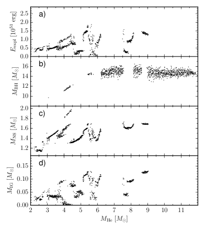
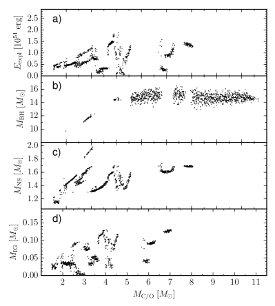
Figure 18: Explosion energy ($E_{\mathrm{expl}}$, Panel a), gravitational remnant mass for black holes ($M_{\mathrm{BH}}$, Panel b) and neutron stars ($M_{\mathrm{NS}}$, sub-panel c), and the iron-group mass ($M_{\mathrm{IG}}$, Panels d) as a function of the helium core mass ($M_{\mathrm{He}}$ left) and the C/O core mass ($M_{\mathrm{C/O}}$, right) at collapse for the standard case. Note that there is a gap in our set of progenitors around $11\,M_{\odot}$; missing data points in this region are not indicative of black hole formation.

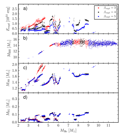
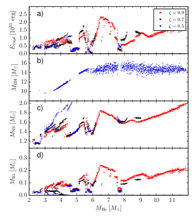
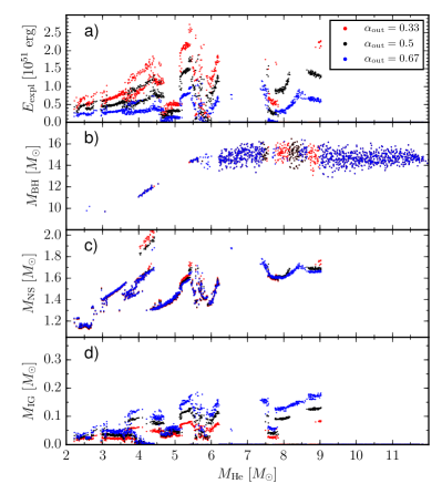
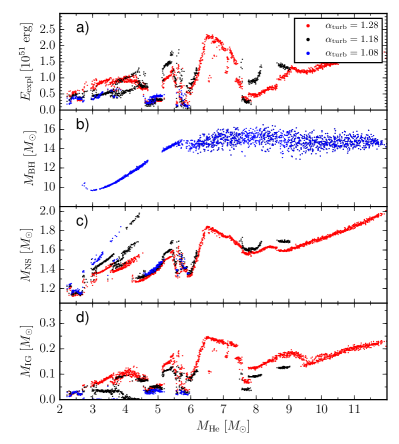
Figure 19: Dependence of the landscape of explosion energies ($E_{\mathrm{expl}}$, Panels a), gravitational remnant masses for black holes ($M_{\mathrm{BH}}$, Panels b) and neutron stars ($M_{\mathrm{NS}}$, Panels c), and iron-group masses ($M_{\mathrm{IG}}$, Panels d) on the shock compression ratio ($\beta_{\mathrm{expl}}$, top left), the efficiency factor for the accretion luminosity ($\zeta$, top right), the outflow surface fraction ($\alpha_{\mathrm{out}}$, bottom left), and the factor for additional shock expansion due to higher turbulent pressure ($\alpha_{\mathrm{turb}}$, bottom right). Different from Figure 13, the explosion parameters are given as a function of helium core mass at collapse, $M_{\mathrm{He}}$, instead of ZAMS mass.

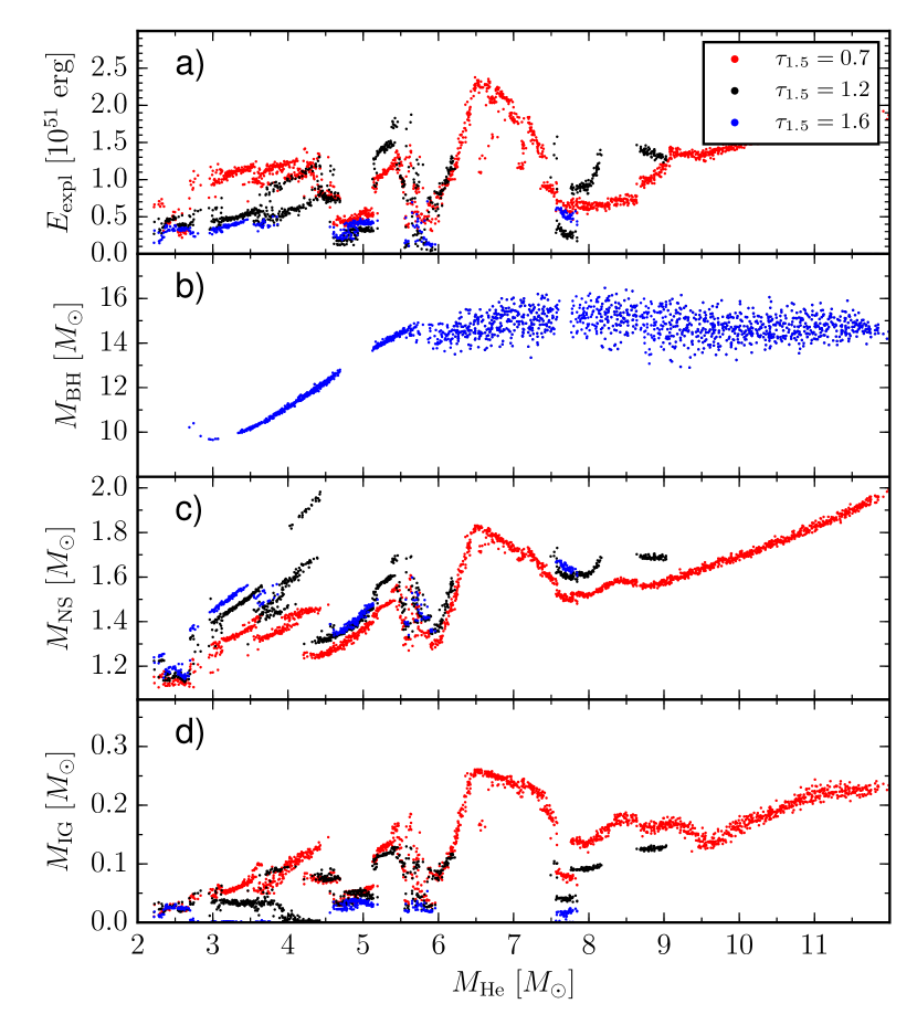
Figure 20: Dependence of the landscape of explosion energies ($E_{\mathrm{expl}}$, Panel a), gravitational remnant masses for black holes ($M_{\mathrm{BH}}$, Panel b) and neutron stars ($M_{\mathrm{NS}}$, Panel c), and iron-group masses ($M_{\mathrm{IG}}$, Panel d) on the cooling time-scale $\tau_{\mathrm{1.5}}$ for a $1.5\,M_{\odot}$ neutron star. Different from Figure 14, the explosion parameters are given as a function of helium core mass at collapse, $M_{\mathrm{He}}$, instead of ZAMS mass.

Figure 21: Compactness parameters, $\xi_{2.5}$, for exploding (red) and non-exploding (black) models as a function of helium core mass $M_{\mathrm{He}}$ at collapse instead of ZAMS mass as in Figure 6. Blue dots denote models where shock revival is initiated, but the explosion eventually fails because the diagnostic energy becomes negative as the shock propagates out or the neutron star mass exceeds the maximum neutron star mass due to ongoing accretion in the explosion phase.

References

- Antoniadis et al. (2013) Antoniadis J., et al., 2013, Science, 340, 448
- Arnett (1996) Arnett D., 1996, Supernovae and Nucleosynthesis: An Investigation of the History of Matter from the Big Bang to the Present
- Asplund et al. (2009) Asplund M., Grevesse N., Sauval A. J., Scott P., 2009, ARA&A, 47, 481
- Beacom (2010) Beacom J. F., 2010, Annual Review of Nuclear and Particle Science, 60, 439
- Belczynski et al. (2008) Belczynski K., Kalogera V., Rasio F. A., Taam R. E., Zezas A., Bulik T., Maccarone T. J., Ivanova N., 2008, ApJS, 174, 223
- Belczynski et al. (2012) Belczynski K., Wiktorowicz G., Fryer C. L., Holz D. E., Kalogera V., 2012, ApJ, 757, 91
- Blinnikov et al. (2000) Blinnikov S., Lundqvist P., Bartunov O., Nomoto K., Iwamoto K., 2000, ApJ, 532, 1132
- Botticella et al. (2012) Botticella M. T., Smartt S. J., Kennicutt R. C., Cappellaro E., Sereno M., Lee J. C., 2012, A&A, 537, A132
- Bruenn et al. (2013) Bruenn S. W., et al., 2013, ApJ, 767, L6
- Bruenn et al. (2016) Bruenn S. W., et al., 2016, ApJ, 818, 123
- Buras et al. (2006) Buras R., Janka H.-T., Rampp M., Kifonidis K., 2006, A&A, 457, 281
- Burrows & Goshy (1993) Burrows A., Goshy J., 1993, ApJ, 416, L75+
- Burrows et al. (1995) Burrows A., Hayes J., Fryxell B. A., 1995, ApJ, 450, 830
- Burrows et al. (2012) Burrows A., Dolence J. C., Murphy J. W., 2012, ApJ, 759, 5
- Cardall & Budiardja (2015) Cardall C. Y., Budiardja R. D., 2015, ApJ, 813, L6
- Chevalier (1989) Chevalier R. A., 1989, ApJ, 346, 847
- Chugai & Utrobin (2014) Chugai N. N., Utrobin V. P., 2014, Astronomy Letters, 40, 291
- Clausen et al. (2015) Clausen D., Piro A. L., Ott C. D., 2015, ApJ, 799, 190
- Couch (2013) Couch S. M., 2013, ApJ, 775, 35
- Couch & Ott (2013) Couch S. M., Ott C. D., 2013, ApJ, 778, L7
- Couch et al. (2015) Couch S. M., Chatzopoulos E., Arnett W. D., Timmes F. X., 2015, ApJ, 808, L21
- Demorest et al. (2010) Demorest P. B., Pennucci T., Ransom S. M., Roberts M. S. E., Hessels J. W. T., 2010, Nature, 467, 1081
- Dolence et al. (2013) Dolence J. C., Burrows A., Murphy J. W., Nordhaus J., 2013, ApJ, 765, 110
- Ertl et al. (2016) Ertl T., Janka H.-T., Woosley S. E., Sukhbold T., Ugliano M., 2016, ApJ, 818, 124
- Faucher-Giguère & Kaspi (2006) Faucher-Giguère C.-A., Kaspi V. M., 2006, ApJ, 643, 332
- Fernández (2012) Fernández R., 2012, ApJ, 749, 142
- Fernández (2015) Fernández R., 2015, MNRAS, 452, 2071
- Fischer et al. (2009) Fischer T., Whitehouse S. C., Mezzacappa A., Thielemann F.-K., Liebendörfer M., 2009, A&A, 499, 1
- Fischer et al. (2010) Fischer T., Whitehouse S. C., Mezzacappa A., Thielemann F., Liebendörfer M., 2010, A&A, 517, A80+
- Fryer (1999) Fryer C. L., 1999, ApJ, 522, 413
- Fryer & Kalogera (2001) Fryer C. L., Kalogera V., 2001, ApJ, 554, 548
- Fryer et al. (2012) Fryer C. L., Belczynski K., Wiktorowicz G., Dominik M., Kalogera V., Holz D. E., 2012, ApJ, 749, 91
- Hamuy (2003) Hamuy M., 2003, ApJ, 582, 905
- Handy et al. (2014) Handy T., Plewa T., Odrzywołek A., 2014, ApJ, 783, 125
- Hanke et al. (2012) Hanke F., Marek A., Müller B., Janka H.-T., 2012, ApJ, 755, 138
- Hanke et al. (2013) Hanke F., Müller B., Wongwathanarat A., Marek A., Janka H.-T., 2013, ApJ, 770, 66
- Hansen et al. (2012) Hansen C. J., et al., 2012, A&A, 545, A31
- Hansen et al. (2014) Hansen C. J., Montes F., Arcones A., 2014, ApJ, 797, 123
- Heger & Woosley (2010) Heger A., Woosley S. E., 2010, ApJ, 724, 341
- Heger et al. (2003) Heger A., Fryer C. L., Woosley S. E., Langer N., Hartmann D. H., 2003, ApJ, 591, 288
- Hidaka & Fuller (2007) Hidaka J., Fuller G. M., 2007, Phys. Rev. D, 76, 083516
- Horiuchi et al. (2011) Horiuchi S., Beacom J. F., Kochanek C. S., Prieto J. L., Stanek K. Z., Thompson T. A., 2011, ApJ, 738, 154
- Hüdepohl (2014) Hüdepohl L., 2014, PhD thesis, Technische Universität München
- Hurley et al. (2000) Hurley J. R., Pols O. R., Tout C. A., 2000, MNRAS, 315, 543
- Iliadis (2007) Iliadis C., 2007, Nuclear Physics of Stars. Wiley-VCH Verlag
- Itoh et al. (1996) Itoh N., Hayashi H., Nishikawa A., Kohyama Y., 1996, ApJS, 102, 411
- Janka (2001) Janka H.-T., 2001, A&A, 368, 527
- Janka (2012) Janka H.-T., 2012, Annual Review of Nuclear and Particle Science, 62, 407
- Janka (2013) Janka H.-T., 2013, MNRAS, 434, 1355
- Janka et al. (2008) Janka H.-T., Müller B., Kitaura F. S., Buras R., 2008, A&A, 485, 199
- Janka et al. (2012) Janka H.-T., Hanke F., Hüdepohl L., Marek A., Müller B., Obergaulinger M., 2012, Progress of Theoretical and Experimental Physics, 2012, 010000
- Jerkstrand et al. (2015) Jerkstrand A., et al., 2015, ApJ, 807, 110
- Kasen & Woosley (2009) Kasen D., Woosley S. E., 2009, ApJ, 703, 2205
- Kitaura et al. (2006) Kitaura F. S., Janka H.-T., Hillebrandt W., 2006, A&A, 450, 345
- Kiziltan et al. (2013) Kiziltan B., Kottas A., De Yoreo M., Thorsett S. E., 2013, ApJ, 778, 66
- Kochanek (2015) Kochanek C. S., 2015, MNRAS, 446, 1213
- Lattimer (2012) Lattimer J. M., 2012, Annual Review of Nuclear and Particle Science, 62, 485
- Lattimer & Prakash (2001) Lattimer J. M., Prakash M., 2001, ApJ, 550, 426
- Lattimer & Swesty (1991) Lattimer J. M., Swesty F. D., 1991, Nucl.~Phys.~A, 535, 331
- Lattimer & Yahil (1989) Lattimer J. M., Yahil A., 1989, ApJ, 340, 426
- Lentz et al. (2015) Lentz E. J., et al., 2015, ApJ, 807, L31
- Liebendörfer et al. (2009) Liebendörfer M., Whitehouse S. C., Fischer T., 2009, ApJ, 698, 1174
- Litvinova & Nadezhin (1985) Litvinova I. Y., Nadezhin D. K., 1985, Soviet Astronomy Letters, 11, 145
- Lovegrove & Woosley (2013) Lovegrove E., Woosley S. E., 2013, ApJ, 769, 109
- Marek & Janka (2009) Marek A., Janka H., 2009, ApJ, 694, 664
- Matzner & McKee (1999) Matzner C. D., McKee C. F., 1999, ApJ, 510, 379
- Melson et al. (2015a) Melson T., Janka H.-T., Marek A., 2015a, ApJ, 801, L24
- Melson et al. (2015b) Melson T., Janka H.-T., Bollig R., Hanke F., Marek A., Müller B., 2015b, ApJ, 808, L42
- Müller (2015) Müller B., 2015, MNRAS, 453, 287
- Müller & Janka (2014) Müller B., Janka H.-T., 2014, ApJ, 788, 82
- Müller & Janka (2015) Müller B., Janka H.-T., 2015, MNRAS, 448, 2141
- Müller et al. (2012a) Müller B., Janka H.-T., Marek A., 2012a, ApJ, 756, 84
- Müller et al. (2012b) Müller B., Janka H.-T., Heger A., 2012b, ApJ, 761, 72
- Müller et al. (2013) Müller B., Janka H.-T., Marek A., 2013, ApJ, 766, 43
- Murphy & Burrows (2008) Murphy J. W., Burrows A., 2008, ApJ, 688, 1159
- Murphy et al. (2013) Murphy J. W., Dolence J. C., Burrows A., 2013, ApJ, 771, 52
- Nadezhin (1980) Nadezhin D. K., 1980, Ap&SS, 69, 115
- Nakamura et al. (2015) Nakamura K., Takiwaki T., Kuroda T., Kotake K., 2015, PASJ, 67, 107
- Ng & Romani (2007) Ng C.-Y., Romani R. W., 2007, ApJ, 660, 1357
- O’Connor & Couch (2015) O’Connor E., Couch S., 2015, preprint, (arXiv:1511.07443)
- O’Connor & Ott (2011) O’Connor E., Ott C. D., 2011, ApJ, 730, 70
- O’Connor & Ott (2013) O’Connor E., Ott C. D., 2013, ApJ, 762, 126
- Özel et al. (2010) Özel F., Psaltis D., Narayan R., McClintock J. E., 2010, ApJ, 725, 1918
- Özel et al. (2012) Özel F., Psaltis D., Narayan R., Santos Villarreal A., 2012, ApJ, 757, 55
- Pejcha & Prieto (2015) Pejcha O., Prieto J. L., 2015, ApJ, 799, 215
- Pejcha & Thompson (2012) Pejcha O., Thompson T. A., 2012, ApJ, 746, 106
- Pejcha & Thompson (2015) Pejcha O., Thompson T. A., 2015, ApJ, 801, 90
- Perego et al. (2015) Perego A., Hempel M., Fröhlich C., Ebinger K., Eichler M., Casanova J., Liebendoerfer M., Thielemann F.-K., 2015, ApJ, 806, 275
- Podsiadlowski & Joss (1989) Podsiadlowski P., Joss P. C., 1989, Nature, 338, 401
- Podsiadlowski et al. (1990) Podsiadlowski P., Joss P. C., Rappaport S., 1990, A&A, 227, L9
- Popov (1993) Popov D. V., 1993, ApJ, 414, 712
- Poznanski (2013) Poznanski D., 2013, MNRAS, 436, 3224
- Rampp & Janka (2002) Rampp M., Janka H.-T., 2002, A&A, 396, 361
- Rauscher et al. (2002) Rauscher T., Heger A., Hoffman R. D., Woosley S. E., 2002, ApJ, 576, 323
- Repetto et al. (2012) Repetto S., Davies M. B., Sigurdsson S., 2012, MNRAS, 425, 2799
- Scheck et al. (2006) Scheck L., Kifonidis K., Janka H.-T., Müller E., 2006, A&A, 457, 963
- Schwab et al. (2010) Schwab J., Podsiadlowski P., Rappaport S., 2010, ApJ, 719, 722
- Shapiro & Teukolsky (1983) Shapiro S. L., Teukolsky S. A., 1983, Black Holes, White Dwarfs, and Neutron Stars: The Physics of Compact Objects. Wiley-Interscience, New York
- Shigeyama & Nomoto (1990) Shigeyama T., Nomoto K., 1990, ApJ, 360, 242
- Smartt (2009) Smartt S. J., 2009, ARA&A, 47, 63
- Smartt (2015) Smartt S. J., 2015, Publ. Astron. Soc. Australia, 32, 16
- Smartt et al. (2009) Smartt S. J., Eldridge J. J., Crockett R. M., Maund J. R., 2009, MNRAS, 395, 1409
- Sukhbold & Woosley (2014) Sukhbold T., Woosley S. E., 2014, ApJ, 783, 10
- Sukhbold et al. (2016) Sukhbold T., Ertl T., Woosley S. E., Brown J. M., Janka H.-T., 2016, ApJ, 821, 38
- Summa et al. (2015) Summa A., Hanke F., Janka H.-T., Melson T., Marek A., Müller B., 2015, preprint, (arXiv:1511.07871)
- Suwa et al. (2010) Suwa Y., Kotake K., Takiwaki T., Whitehouse S. C., Liebendörfer M., Sato K., 2010, PASJ, 62, L49+
- Suwa et al. (2016) Suwa Y., Yamada S., Takiwaki T., Kotake K., 2016, ApJ, 816, 43
- Takiwaki et al. (2012) Takiwaki T., Kotake K., Suwa Y., 2012, ApJ, 749, 98
- Takiwaki et al. (2014) Takiwaki T., Kotake K., Suwa Y., 2014, ApJ, 786, 83
- Tamborra et al. (2014) Tamborra I., Hanke F., Janka H.-T., Müller B., Raffelt G. G., Marek A., 2014, ApJ, 792, 96
- Tanaka et al. (2009) Tanaka M., et al., 2009, ApJ, 692, 1131
- Tauris et al. (2011) Tauris T. M., Langer N., Kramer M., 2011, MNRAS, 416, 2130
- Thompson (2000) Thompson C., 2000, ApJ, 534, 915
- Thompson et al. (2005) Thompson T. A., Quataert E., Burrows A., 2005, ApJ, 620, 861
- Ting et al. (2012) Ting Y.-S., Freeman K. C., Kobayashi C., De Silva G. M., Bland-Hawthorn J., 2012, MNRAS, 421, 1231
- Travaglio et al. (2004) Travaglio C., Gallino R., Arnone E., Cowan J., Jordan F., Sneden C., 2004, ApJ, 601, 864
- Ugliano et al. (2012) Ugliano M., Janka H.-T., Marek A., Arcones A., 2012, ApJ, 757, 69
- Utrobin (1993) Utrobin V., 1993, A&A, 270, 249
- Utrobin (2005) Utrobin V. P., 2005, Astronomy Letters, 31, 806
- Weaver et al. (1978) Weaver T. A., Zimmerman G. B., Woosley S. E., 1978, ApJ, 225, 1021
- Woosley & Heger (2007) Woosley S. E., Heger A., 2007, Phys. Rep., 442, 269
- Woosley & Heger (2015a) Woosley S. E., Heger A., 2015a, ApJ, 806, 145
- Woosley & Heger (2015b) Woosley S. E., Heger A., 2015b, ApJ, 810, 34
- Woosley & Weaver (1995) Woosley S. E., Weaver T. A., 1995, ApJS, 101, 181
- Woosley et al. (1973) Woosley S. E., Arnett W. D., Clayton D. D., 1973, ApJS, 26, 231
- Woosley et al. (2002) Woosley S. E., Heger A., Weaver T. A., 2002, Rev.~Mod.~Phys., 74, 1015
- Zhang et al. (2008) Zhang W., Woosley S. E., Heger A., 2008, ApJ, 679, 639
- von Groote (2014) von Groote J., 2014, PhD thesis, Technische Universität München